Phase transition in peristaltic transport of frictionless granular particles

Abstract

Flows of dissipative particles driven by the peristaltic motion of a tube are numerically studied. A transition from a slow “unjammed” flow to a fast “jammed” flow is found through the observation of the flow rate at a critical width of the bottleneck of a peristaltic tube. It is also found that the average and fluctuation of the transition time, and the peak value of the second moment of the flow rate exhibit power-law divergence near the critical point and that these variables satisfy scaling relationships near the critical point. The dependence of the critical width and exponents on the peristaltic speed and the density is also discussed.

I Introduction

Peristalsis is a progressive wave of area contraction and expansion in a tube. Transport due to the peristaltic motion of a tube is one of the main transport mechanisms in biological systems such as the esophagus, small intestine, ureter, and so forth Jaffrin and Shapiro (1971). Peristaltic transport is also found in the pumping of fluids, known as peristaltic pumps, which are employed in medical and food engineering fields Jaffrin and Shapiro (1971).

The study of peristaltic transport has a long history and was particularly motivated by the desire to understand the transport of fluids in the ureter. Peristaltic transport in a Stokes fluid was studied in the late 1960s Burns and Parkes (1967); Shapiro et al. (1969) and early 1970s Li (1970); Yin and Fung (1971); Weinberg et al. (1971). A study on the peristaltic transport of a micropolar fluid Srinivasacharya et al. (2003) following this direction has also been reported. In contrast, there have been few studies on the transport of particles under a peristaltic condition such as single particles Hung and Brown (1976); Fauci (1992) and dilute passive solid particles Jiménez-Lozano et al. (2009); Jiménez-Lozano and Sen (2010) suspended in a Newtonian fluid. Moreover, to the best of our knowledge, the peristaltic transport of dense particles has never been studied, even though such a situation is commonly observed in flows of red blood cells, in the peristaltic pumping of corrosive sand and solid foods, and so forth Jaffrin and Shapiro (1971).

Here, we consider the peristaltic transport of dry and smooth granular particles, which is closely related to the transport of particles through a bottleneck Helbing (2001); Nakajima and Hayakawa (2009), particularly the discharge of grains from a silo Le Pennec et al. (1996); Longhi et al. (2002); Beverloo et al. (1961); Nedderman et al. (1982); Mankoc et al. (2007); De-Song et al. (2003); Aguirre et al. (2010); Hou et al. (2003); Zhong et al. (2006); Huang et al. (2006); Janda et al. (2009); To et al. (2001); To (2005); Zuriguel et al. (2003, 2005); Janda et al. (2008). Through previous studies it has been established that there are three regimes depending on the linear size of the bottleneck, $w$. If $w$ is sufficiently large, particles flow continuously Beverloo et al. (1961); Nedderman et al. (1982); Mankoc et al. (2007); De-Song et al. (2003); Aguirre et al. (2010). It is also known that the mass flow rate $Q$ satisfies the Beverloo law $Q\propto(w-w_{0})^{B}$ for an empirical value $w_{0}$, where $B$ is $3/2$ and $5/2$ for two- and three-dimensional systems under gravity, respectively Beverloo et al. (1961); Nedderman et al. (1982); Mankoc et al. (2007), and $B$ is $1$ for disks on a conveyor belt De-Song et al. (2003); Aguirre et al. (2010). With decreasing size of the bottleneck, the flow becomes intermittent owing to the formation and breakdown of an arch at the outlet Hou et al. (2003); Zhong et al. (2006); Huang et al. (2006); Janda et al. (2009), and finally the flow stops, i.e., jamming occurs To et al. (2001); To (2005); Zuriguel et al. (2003, 2005); Janda et al. (2008). Note, however, that the term jamming used in this context is slightly different from that in the jamming transition of granular matter discussed in recent studies O’Hern et al. (2002, 2003); Dauchot et al. (2005); Olsson and Teitel (2007); Hatano (2008); Otsuki and Hayakawa (2009a, b); Otsuki et al. (2010). Indeed, the jamming transition can be observed even for smooth, i.e., frictionless, granular particles, while the jamming of a granular flow at the bottleneck is due to the persistent arch formation by grains, which can be observed only for rough, or frictional, particles. What actually corresponds to the jamming transition in the discharge of grains appears to be the so-called dilute-to-dense transition Hou et al. (2003); Zhong et al. (2006); Huang et al. (2006), which is observed at a phase boundary between continuous and intermittent regimes.

In this paper, we report the results of our simulations on the flow rate of a peristaltic granular flow. We consider dry, smooth, monodisperse, and spherical particles in a three-dimensional sinusoidally oscillating tube. After the introduction of our numerical model in Sec. II, we present the results of our simulations in Sec. III. Through the observation of the flow rate, we find a transition from a slow “unjammed” flow to a fast “jammed” flow occurs if the minimum width of the peristaltic tube is smaller than a critical value. We also find that the average and fluctuation of the transition time, and the peak value of the second moment of the flow rate exhibit power-law divergence with nontrivial exponents near the minimum width. Moreover, we verify the existence of scaling functions for these quantities. It is also found that the critical width is almost independent of the density but depends on peristaltic velocity. In Sec. IV, we discuss and summarize our results.

II Model

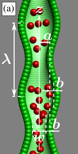
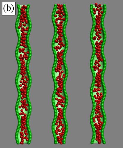
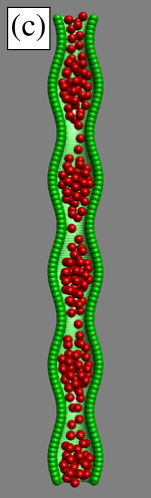
Figure 1: (Color online) (a) Snapshot of our simulation showing some of the parameters in our model. See the text for details. (b) Sequential snapshots of the simulation for ${w}=2.0$, ${\dot{\epsilon}}=1.83\times 10^{-1}$, and $\bar{\rho}=2.96\times 10^{-1}$. Time increases from left to right, and the peristaltic wave of the wall progresses upward. The system remains in the unjammed flow regime when ${{t}}<{\tau}$. (c) Snapshot of stationary state for the parameters used in (b) showing the jammed flow regime when ${{t}}>{\tau}$. Dark (red) spheres and light (green) spheres are transported particles and particles embedded in the wall, respectively. Wall particles facing the reader are not visualized to show the transported particles clearly.

We adopt the three-dimensional molecular dynamics simulation for soft-core particles known as the discrete element method (DEM) to simulate the peristaltic flow of spherical granular particles. We assume that the particles are dry, smooth, and monodisperse spheres. This means that we can ignore tangential forces that lead to the sliding and rotation of particles as well as adhesive forces. We also assume that all the material properties of the particles are identical. Moreover, to idealize our setup, we ignore gravity and the hydrodynamic force through interstitial fluids such as air. Peristaltic motion is represented by the propagation of a spatially oscillating wall along the axial direction of a tube, which is described in detail in the following.

The system involves ${N}$ monodisperse, smooth, and mobile granular spheres with diameter ${{d}}$ and mass ${{m}}$ in a peristaltic tube with length ${L}$ under a periodic boundary condition along the direction of propagation ${{z}}$ of peristaltic waves. The wall of the tube consists of ${N_{\mathrm{w}}}$ embedded overlapping spheres. We ignore interactions among the particles embedded in the wall and the deformation of the wall. Therefore, we assume that the peristaltic wave of the wall is uniform and perfectly controllable. See the schematic diagram shown in Fig. 1 (a).

We label a set of particles ${\Pi_{\mathrm{p}}}=\{1,\ldots,{N}\}$ denoting mobile particles and ${\Pi_{\mathrm{w}}}=\{{N}+1,\ldots,{N}+{N_{\mathrm{w}}}\}$ denoting particles embedded in the wall, where ${N_{\mathrm{w}}}$ is the number of particles embedded in the wall, with the relation ${\Pi}={\Pi_{\mathrm{p}}}\cup{\Pi_{\mathrm{w}}}$. For $i\in\Pi_{\mathrm{p}}$, i.e., mobile particles, the equation of motion is given by

$${{m}}\dfrac{\mathrm{d}^{2}{{{\boldsymbol{r}}_{i}}}}{\mathrm{d}{{{t}}}^{2}}=\sum_{j\in{\Pi},j\neq i}\bigl{(}{{\boldsymbol{f}}^{\mathrm{el}}_{ij}}+{{\boldsymbol{f}}^{\mathrm{vis}}_{ij}}\bigr{)},$$ (1)

where ${{\boldsymbol{f}}^{\mathrm{el}}_{ij}}$ and ${{\boldsymbol{f}}^{\mathrm{vis}}_{ij}}$ are respectively the elastic and viscous contact forces acting on particle $i$ by particle $j$. For their explicit forms, we adopt the following model:

$${{\boldsymbol{f}}^{\mathrm{el}}_{ij}} ={{k}}{{\xi}_{ij}}\Theta({{\xi}_{ij}}){{\boldsymbol{n}}_{ij}},$$ (2)

$${{\boldsymbol{f}}^{\mathrm{vis}}_{ij}} =-{{\eta}}({{\boldsymbol{v}}_{ij}}\cdot{{\boldsymbol{n}}_{ij}})\Theta({{\xi}_{ij}}){{\boldsymbol{n}}_{ij}},$$ (3)

where $\Theta(x)$ is a step function with $\Theta(x)=1$ for $x>0$ and $\Theta(x)=0$ otherwise, ${{k}}$ denotes the spring constant, ${{\eta}}$ is the viscosity, ${{\xi}_{ij}}={{d}}-|{{\boldsymbol{r}}_{ij}}|$, ${{\boldsymbol{r}}_{ij}}={{\boldsymbol{r}}_{i}}-{{\boldsymbol{r}}_{j}}$, ${{\boldsymbol{n}}_{ij}}={{\boldsymbol{r}}_{ij}}/|{{\boldsymbol{r}}_{ij}}|$, and ${{\boldsymbol{v}}_{ij}}={{\boldsymbol{v}}_{i}}-{{\boldsymbol{v}}_{j}}$. We solve Eq. (1) numerically using the Euler method with a fixed time interval of $5.48\times 10^{-2}\sqrt{{{m}}/{{k}}}$ for each step.

As mentioned above, we ignore the mutual deformation of the wall. Therefore, an embedded particle $i\in{\Pi_{\mathrm{w}}}$ in the wall can be characterized by its position in the radial direction $r_{0}(t;z)$ of ${{\boldsymbol{r}}_{i}}=\bigl{(}{{r}_{i}}({{t}};{{z}_{i}}),{{\theta}_{i}},{{z}_{i}}\bigr{)}$ in cylindrical coordinates as

$${{r}_{i}}({{t}};{{z}_{i}})=\biggl{(}{a}+\dfrac{{{d}}}{2}\biggr{)}+{b}\sin\dfrac{2\pi}{{\lambda}}({c}{{t}}+{{z}_{i}})$$ (4)

for a sinusoidal peristaltic wave of the wall with amplitude ${b}$, wavelength ${\lambda}$, phase velocity ${c}$, and average tube radius ${a}$. In contrast, ${{\theta}_{i}}$ and ${{z}_{i}}$ are set to form a nearly hexagonal lattice with lattice constant $l$ on the ${{\theta}}$-${{z}}$ plane. See the appendix for more precise descriptions of ${{\theta}_{i}}$ and ${{z}_{i}}$. We fix $l=0.3\,{{d}}$ throughout this paper to prevent the transported particles from penetrating the tube wall, which means that ${N_{\mathrm{w}}}=9984$, although we set ${N}=50,100,\ldots,600$ in our simulations.

Hereafter, we use dimensionless quantities scaled by the units of mass ${{m}}$, length ${{d}}$, and time $\sqrt{{{m}}/{{k}}}$. For example, the length of the tube, time, and viscosity in dimensionless forms are given by ${L}/{{d}}$, ${{t}}\sqrt{{{k}}/{{m}}}$, and ${{\eta}}/\sqrt{{{m}}{{k}}}$, respectively. Note that we do not introduce any new notations for the dimensionless quantities in the following, and use the same notations as those for the dimensional quantities.

We set ${a}=1.5$, ${L}=50$, ${\lambda}=10$, and ${{\eta}}=5.48\times 10^{-3}$ throughout this paper. The controllable parameters are ${b}$, ${c}$, and ${N}$, but instead we use the minimum width of the peristaltic tube, i.e., the width at the bottleneck,

$${w}\equiv 2({a}-{b}),$$ (5)

the strain rate

$${\dot{\epsilon}}\equiv\dfrac{{c}}{{\lambda}},$$ (6)

and the volume fraction at ${b}=0$,

$$\bar{\rho}\equiv\dfrac{{N}}{6{a}{}^{2}{L}},$$ (7)

as the control parameters in this work. Note that we do not use the volume fraction ${\rho}\equiv{N}/6({a}{}^{2}+{b}{}^{2}/2){L}$ but use $\bar{\rho}$ instead. This is because it is difficult to fix ${\rho}$ in simulations and in real experiments when ${b}$ is changed. It is necessary to change both ${N}$ and ${b}$ at the same time. Moreover, ${b}$ must be changed discretely because ${N}$ is a natural number. In this study, the restitution coefficient of the particles, $e$, is given by $e=\exp\bigl{(}-\pi{{\eta}}/\sqrt{2-{{\eta}}^{2}}\bigr{)}\simeq 0.988$, i.e., the particles are almost elastic Otsuki et al. (2010). Note, however, that such “low” inelasticity or dissipation is necessary to reach a steady state because the energy is input to the system continuously by the peristaltic motion.

III Results

We focus on the behavior of the flow rate ${J}({{t}})$, whose explicit definition will be given in Sec. III.1, under the zero-flow-rate initial condition ${J}(0)=0$. If ${w}$ is sufficiently large, the particles can flow without becoming stuck. We call this an unjammed flow (see Fig. 1 (b)). On the other hand, if ${w}$ is sufficiently small, particles become stuck at bottlenecks, and the stuck particles rise with the wall. We call this a jammed flow (see Fig. 1 (c)). We are interested in the particle behavior for intermediate values of ${w}$. In Sec. III.2, we present the results obtained by fixing $\bar{\rho}$ and changing ${w}$ and ${\dot{\epsilon}}$. Meanwhile, the results obtained by changing $\bar{\rho}$ are given in Sec. III.3. Finally, the results for the second moment of the flow rate are reported in Sec. III.4.

It is noteworthy that the terminology of “jammed” and “unjammed” flows is counter-intuitive, because a jammed flow has a larger flow rate than an unjammed flow. This can be understood easily by considering the process relative to a frame moving with the wall. Indeed, the jammed state does not exhibit any motion in this frame, while the unjammed state has some mobile particles moving in the backward direction. Namely, some particles left behind by the wall motion contribute to the negative flow rate in the unjammed phase.

III.1 Definition of flow rate

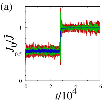
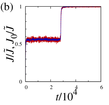
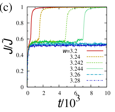
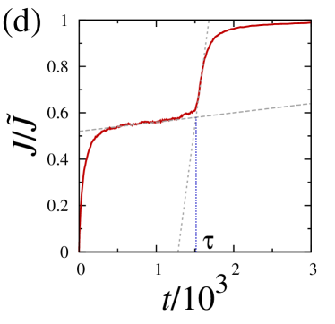
Figure 2: (Color online) (a) Time evolutions of the normalized flow rate ${J}_{0}({{t}},\Delta{{t}})/{\tilde{J}}$ with $\tilde{J}\equiv Nc/L$ for ${w}=2.2448$, ${\dot{\epsilon}}=1.83\times 10^{-1}$, and $\bar{\rho}=2.96\times 10^{-1}$. The definition of ${J}_{0}({{t}},\Delta{{t}})$ is given by Eq. (9). The observation times $\Delta{{t}}$ for ${J}_{0}({{t}},\Delta{{t}})$ are set to $T$, $2T$, and $5T$, where $T=5.48$ is the period of the peristaltic wave. (b) Time evolutions of the normalized flow rates ${J}({{t}})/{\tilde{J}}$ and ${J}_{0}({{t}},5T)/{\tilde{J}}$. The parameters are the same as those in (a). (c) Typical time evolution of normalized flow rate ${J}/{\tilde{J}}$ with ${\dot{\epsilon}}=1.83\times 10^{-1}$ and $\bar{\rho}=2.96\times 10^{-1}$. (d) Same plot as (c) for ${w}=3.24$ to show the definition of the transition time ${\tau}$. See text for details.

The flow rate is often defined Evans and Morriss (1990) as

$${J}({{t}})\equiv\dfrac{1}{{L}}\sum_{i\in{\Pi_{\mathrm{p}}}}{{p}_{i,{{z}}}}({{t}})$$ (8)

in studies employing molecular dynamics simulations and discrete element methods, where ${{p}_{i,{{z}}}}({{t}})$ is the ${{z}}$-component of the dimensionless momentum of particle $i$. In real experiments, however, the above definition may not be appropriate because it requires the momenta of all particles. Instead, the following definition is usually used:

$${J}_{{{z}}^{\prime}}({{t}},\Delta{{t}})\equiv\dfrac{\Delta{N}_{{{z}}^{\prime}}({{t}},\Delta{{t}})}{\Delta{{t}}},$$ (9)

where $\Delta{N}_{{{z}}^{\prime}}({{t}},\Delta{{t}})$ is a signed number of particles passing a section ${{z}}={{z}}^{\prime}$ during the time interval $[{{t}},{{t}}+\Delta{{t}})$, with $+1$ counted if a particle passes from ${{z}}<{{z}}^{\prime}$ to ${{z}}>{{z}}^{\prime}$ and $-1$ counted for the opposite case. Therefore, we first check that the definition given by Eq. (8) is in agreement with that given by Eq. (9).

Figure 2 (a) plots time evolutions of the flow rate ${J}_{z^{\prime}=0}({{t}},\Delta{{t}})$ normalized by ${\tilde{J}}={N}{c}/{L}$. Note that if all particles rise with the wall, i.e., ${{\boldsymbol{v}}_{i}}=(0,0,{c})$ for every particle $i$, ${J}$ is equal to ${\tilde{J}}$. It is clearly shown that the fluctuation of the curve decreases as $\Delta{{t}}$ increases. Moreover, Fig. 2 (b) shows time evolutions of the normalized flow rates ${J}({{t}})/{\tilde{J}}$ and ${J}_{0}({{t}},5T)/{\tilde{J}}$, where $T\equiv{\lambda}/{c}=1/{\dot{\epsilon}}$. From these figures, we confirm that ${J}_{0}({{t}},\Delta t)$ converges to ${J}({{t}})$ for sufficiently large $\Delta t$. Therefore, if one is not interested in short-time behavior, Eq. (8) can be used for data analysis. Hereafter, we adopt Eq. (8) for the flow rate in the subsequent discussion.

III.2 Transition between jammed and unjammed flow

Figure 2 (c) shows a typical example of the time evolution of the flow rate ${J}/{\tilde{J}}$ for various ${w}$. It is clearly shown that, while an almost stationary and slow unjammed flow continues for large ${w}$, a transition from a slow unjammed flow to a fast jammed flow occurs for small ${w}.$

We introduce the transition time ${\tau}$ to characterize the transition from the unjammed flow to the jammed flow (Fig. 2 (c)). First, we linearly fit the curve of the flow rate before a transition (gentle dashed line). We again fit the curve after the transition in a similar way (steep dashed line). Then the transition time is defined as the time at which these two fitted lines cross. Note that the transition time in this definition is not the lifetime of a metastable state but the relaxation time from the start of the unjammed flow. Such a definition is commonly used to characterize the relaxation from metastable states in melting dynamics Binder (1973) and the so-called $\alpha$-relaxation in glass transitions Kob and Andersen (1994, 1995).

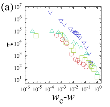
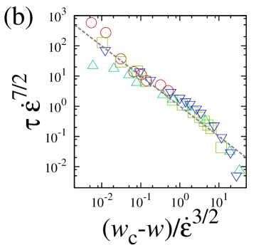
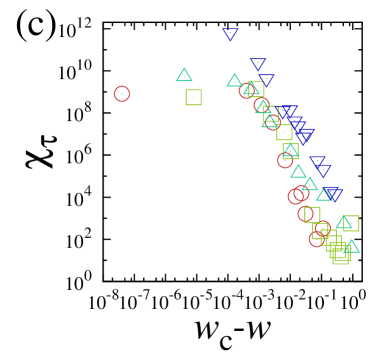
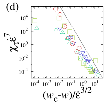
Figure 3: (Color online) (a) Transition time ${\tau}$ as a function of ${w_{\mathrm{c}}}-{w}$. (b) Scaling function $f(x)$ with $x=({w_{\mathrm{c}}}-{w})/{\dot{\epsilon}}{}^{\nu}$ and $\nu=3/2$; see Eq. (10). (c) Fluctuation of transition time ${\chi_{\tau}}$ as a function of ${w_{\mathrm{c}}}-{w}$. (d) Scaling function $g(x)$ with $x=({w_{\mathrm{c}}}-{w})/{\dot{\epsilon}}{}^{\nu}$; see Eq. (11). For all figures, we use the density $\bar{\rho}=2.96\times 10^{-1}$, and circles, squares, triangles, and inverted triangles correspond to the data for ${\dot{\epsilon}}=3.65\times 10^{-1},1.83\times 10^{-1},9.13\times 10^{-2}$, and $4.56\times 10^{-2}$, respectively.

Figure 3 (a) shows the ${w}$-dependence of ${\tau}$ for various ${\dot{\epsilon}}$, which suggests the existence of a power law between $\tau$ and $w_{c}-w$. Although it may be difficult to extract a universal feature from Fig. 3 (a), the data may satisfy the scaling form

$${\tau}\simeq{\dot{\epsilon}}{}^{-\zeta}f\bigl{(}({w_{\mathrm{c}}}-{w})/{\dot{\epsilon}}{}^{\nu}\bigr{)},$$ (10)

where $f(x)\sim x^{-{\alpha}}$ for $x\sim 1$ and might undergo exponential decay for $x\gg 1$ (see Fig. 3 (b)). Note that the critical width $w_{c}$ is determined from Eq. (10). This is because the raw data obtained from the simulation, as shown in Fig. 3 (a), cannot reach the critical point within our simulation time. From Fig. 3 (b), we numerically obtain ${\alpha}=1$, $\nu=3/2$, and $\zeta=7/2$ for $\bar{\rho}=2.96\times 10^{-1}$. The existence of the scaling law given by Eq. (10) suggests that this jamming transition is analogous to the conventional second-order phase transition.

We also study the ${w}$-dependence of the fluctuation of the transition time ${\chi_{\tau}}\equiv\langle{\tau}{}^{2}\rangle-\langle{\tau}\rangle^{2}$. We again find, as shown in Figs. 3 (c) and (d), the existence of the scaling form

$${\chi_{\tau}}\simeq{\dot{\epsilon}}{}^{-2\zeta}g\bigl{(}({w_{\mathrm{c}}}-{w})/{\dot{\epsilon}}{}^{\nu}\bigr{)},$$ (11)

where $g(x)\sim x^{-\beta}$ for $x\sim 1$ and might undergo exponential decay for $x\gg 1$. The value of $\beta$ is approximately equal to $3$ for $\bar{\rho}=2.96\times 10^{-1}$.

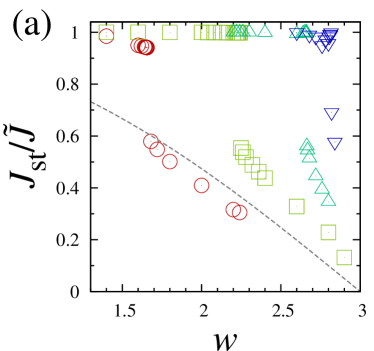
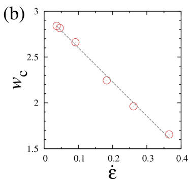
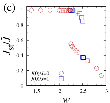
Figure 4: (Color online) (a) Normalized stationary flow rate ${J_{\mathrm{st}}}/{\tilde{J}}$ as a function of ${w}$ for $\bar{\rho}=2.96\times 10^{-1}$ and various ${\dot{\epsilon}}$, where the dashed line is given by Eq. (13). The symbols are the same as those in Fig. 3. (b) Plot of ${w_{\mathrm{c}}}$ as a function of ${\dot{\epsilon}}$ for $\bar{\rho}=2.96\times 10^{-1}$. (c) Hysteresis loop of flow rate for $\bar{\rho}=2.96\times 10^{-1}$ and ${\dot{\epsilon}}=1.83\times 10^{-1}$. Circles and squares correspond to ${J_{\mathrm{st}}}/{\tilde{J}}=0$ and $1$, respectively.

We now discuss how ${w_{\mathrm{c}}}$ depends on ${\dot{\epsilon}}$. Figure 4 (a) shows the ${w}$-dependence of ${J_{\mathrm{st}}}/{\tilde{J}}$, where ${J_{\mathrm{st}}}$ is the stationary flow rate of the jammed flow for ${w}<{w_{\mathrm{c}}}$ or that of the unjammed flow for ${w}>{w_{\mathrm{c}}}$. There is a jump in each stationary flow rate ${J_{\mathrm{st}}}$ at ${w}={w_{\mathrm{c}}}({\dot{\epsilon}})$. The transition point ${w_{\mathrm{c}}}({\dot{\epsilon}})$ strongly depends on ${\dot{\epsilon}}$ as shown in Fig. 4 (b). This figure shows that ${w_{\mathrm{c}}}$ linearly increases with decreasing ${\dot{\epsilon}}$ as

$${w_{\mathrm{c}}}({\dot{\epsilon}})\simeq-3.75{\dot{\epsilon}}+{w_{\mathrm{max}}},$$ (12)

at least for ${\dot{\epsilon}}<0.4$.

The jump in the stationary flow rate may imply that the jamming transition is not continuous but discontinuous, although the scaling forms given by Eqs. (10) and (11) are usually a characteristic of a continuous transition. To determine whether our jamming transition is continuous or discontinuous, we have investigated whether there is hysteresis in the vicinity of the transition point. Figure 4 (c) illustrates the existence of a hysteresis loop of the flow rate for $\bar{\rho}=2.96\times 10^{-1}$ and ${\dot{\epsilon}}=1.83\times 10^{-1}$, which is clear evidence that this jamming transition is discontinuous. In the figure, squares and circles correspond to data obtained from simulations with the initial conditions ${J}(0)={\tilde{J}}$ and $J(0)=0$, respectively. For $J(0)=\tilde{J}$, there is a stable and steady jammed flow for ${w}<{w_{\mathrm{c}}^{\prime}}$, a transition from the jammed flow to the unjammed flow takes place at $w=w_{c}^{\prime}$, and the unjammed flow is stable for ${w}>{w_{\mathrm{c}}^{\prime}}$. It is clear that the transition point ${w_{\mathrm{c}}^{\prime}}$ satisfies $w_{c}^{\prime}>{w_{\mathrm{c}}}$.

It is well known that the transition time or relaxation time from a metastable state to a stable equilibrium state diverges at a critical point for a discontinuous phase transition Binder (1973, 1987); Krzakala and Zdeborova (2011a, b). One commonly observes that the Vogel-Fulcher-Tammann law, or its variant $\tau\sim\exp(-C\delta^{-\gamma})$, is satisfied for the relaxation time, where $\delta$ is a rescaled control parameter or the distance from the critical or spinodal point. Meanwhile, the power-law divergence $\tau\sim\delta^{-\alpha}$ is also often observed near the spinodal point in mean-field models Binder (1973, 1987); Krzakala and Zdeborova (2011a, b) and in molecular dynamics simulations for sheared colloidal systems Miyama and Sasa (2011). Our system is another example of a system in which the transition time to a stable state exhibits power-law divergence at a critical point as $\tau\sim\delta^{-\alpha}$, with $\delta=1-{w}/{w_{\mathrm{c}}}$ and $\alpha=1$ for a nonequilibrium discontinuous phase transition.

We also investigate the dependence of the stationary flow rate on ${w}$ in the jammed and unjammed flow phases. The dashed curve in Fig. 4 (a) shows the analytic relation between the stationary flow rate $J_{\rm st}^{\rm fluid}$ and the minimum width in a Stokes fluid under an infinite wavelength limit Jaffrin and Shapiro (1971),

$$\dfrac{{J_{\mathrm{st}}^{\mathrm{fluid}}}}{{\tilde{J}}}=\dfrac{3\phi}{2+\phi^{2}}=\dfrac{3(1-{w}/{a})}{2+(1-{w}/{a})^{2}},$$ (13)

where $\phi={b}/{a}=1-{w}/{a}$. In the jammed flow phase with ${w}<{w_{\mathrm{c}}}$, the stationary flow rate is almost independent of ${w}$ and, as expected, does not follow Eq. (13). On the other hand, the flow rate decreases as $w$ increases in the unjammed flow phase with ${w}>{w_{\mathrm{c}}}$. It is surprising that the functional form of the stationary flow rate is similar to Eq. (13) for large $\dot{\epsilon}$, e.g., $\dot{\epsilon}=0.365$ (see Fig. 4 (a)), although the flow rate is larger for smaller $\dot{\epsilon}$. This is counter-intuitive because the Reynolds number is usually defined as $Re={a}^{2}{c}/\nu{\lambda}$ with kinematic viscosity $\nu$, and thus, the flow rate converges to Eq. (13) as ${\dot{\epsilon}}\to 0$ in the case of a Stokes flow Jaffrin and Shapiro (1971); Shapiro et al. (1969); Weinberg et al. (1971); Jaffrin (1973). A means of solving this puzzle might be to consider the effect of compressibility. Indeed, it is known that the stationary flow rate increases as ${c}$ decreases if ${c}$ is greater than the sound velocity Aarts and Ooms (1998); Felderhof (2011). It is also known that a granular fluid is compressible Brilliantov and Pöschel (2004). Of course, the existence of a role of incompressibility raises an interesting question: why is the behavior of a suspension flow in an incompressible fluid similar to that of a Stokes flow? At present, this is an open question.

III.3 Density dependence

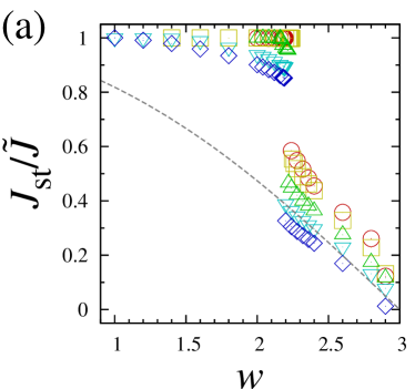
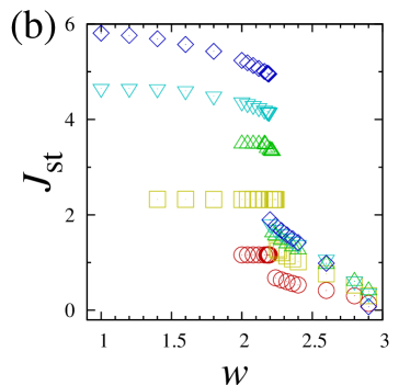
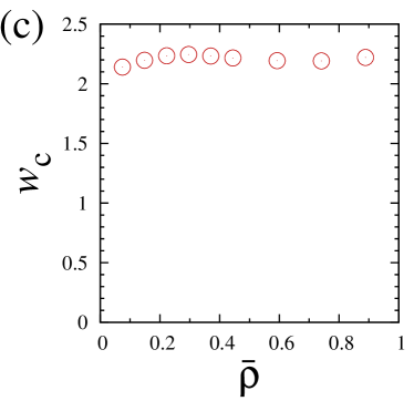
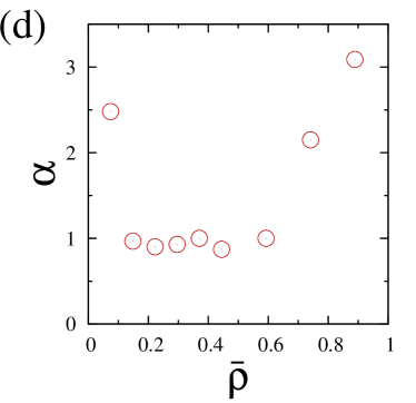
Figure 5: (Color online) (a) Normalized stationary flow rate ${J_{\mathrm{st}}}/{\tilde{J}}$ as a function of ${w}$ for various $\bar{\rho}$. The dashed line shows Eq. (13). Circles, squares, triangles, inverted triangles, and diamonds correspond to $\bar{\rho}=1.48\times 10^{-1},2.96\times 10^{-1},4.44\times 10^{-1},5.92\times 10^{-1}$, and $7.40\times 10^{-1}$, respectively. (b) Unnormalized stationary flow rate. (c) Plot of ${w_{\mathrm{c}}}$ as a function of $\bar{\rho}$. (d) Plot of ${\alpha}$ as a function of $\bar{\rho}$. All figures are obtained for ${\dot{\epsilon}}=1.83\times 10^{-1}$.

In this subsection we investigate how the flow rate depends on the density under a fixed strain rate of ${\dot{\epsilon}}=1.83\times 10^{-1}$. Figures 5 (a) and (b) show the normalized and unnormalized stationary flow rates ${J_{\mathrm{st}}}/{\tilde{J}}$ and ${J_{\mathrm{st}}}$ as functions of ${w}$ for various $\bar{\rho}$, respectively. Although the actual flow rate $J_{\rm st}$ increases as the density increases (Fig. 5 (b)), the normalized flow rate decreases with increasing density (Fig. 5 (a)). For the jammed flow phase, ${w}<{w_{\mathrm{c}}}$, with relatively large $\bar{\rho}$, there are some particles that do not move with the wall. Note that the transition point ${w_{\mathrm{c}}}\simeq 2.2$ is almost independent of the density as shown in Fig. 5 (c).

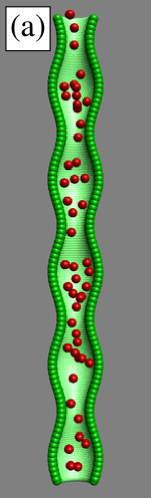
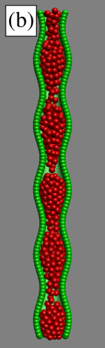
Figure 6: (Color online) (a) Snapshot of stationary state for ${w}=2.0$, ${\dot{\epsilon}}=1.83\times 10^{-1}$, and $\bar{\rho}=7.40\times 10^{-2}$. Although particles do not become stuck at bottlenecks, the stationary flow rate ${J_{\mathrm{st}}}$ reaches ${\tilde{J}}$. (b) Snapshot of stationary state for ${w}=2.0$, ${\dot{\epsilon}}=1.83\times 10^{-1}$, and $\bar{\rho}=7.40\times 10^{-1}$.

We also demonstrate that the exponent ${\alpha}$ is a constant for $0.15\lesssim\bar{\rho}\lesssim 0.60$ in Fig. 5 (d). For a dilute gas with $\bar{\rho}\lesssim 0.10$, ${\alpha}$ is much larger than $1$. This might be because the transport of particles is not determined by the rare collisions between particles but by the direct momentum transfer from the peristaltic wave of the wall (Fig. 6 (a)). On the other hand, ${\alpha}$ is also larger than unity for $\bar{\rho}\gtrsim 0.70$. This might be related to the insufficient free volume around the antinodes of the tube (Fig. 6 (b)). Particles passing through a bottleneck soon collide with other jammed particles around the next antinode and thus they are deflected. These deflected particles may affect the configuration of jammed particles near the bottleneck. Because we focus on the appearance of the jammed flow, we can state that the relationship ${\alpha}\simeq 1$ is always held for a wide range of densities.

The dashed curve in Fig. 5 (a) shows Eq. (13) or the ${w}$-dependence of the flow rate in a Stokes fluid. We find that the flow rate in the unjammed flow phase becomes increasingly close to that given by Eq. (13) with increasing density $\bar{\rho}$. This also indicates that compressibility has a crucial role in causing the functional form of ${J_{\mathrm{st}}}/{\tilde{J}}$ to deviate from Eq. (13). It is also worth noting that ${J_{\mathrm{st}}}/{\tilde{J}}$ is not constant in the jammed phase if $\bar{\rho}$ is sufficiently high.

III.4 Second moment of flow rate

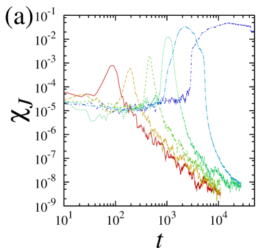
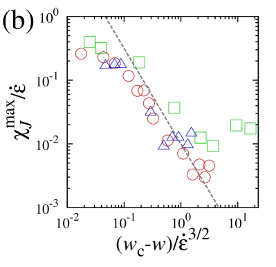
Figure 7: (Color online) (a) Second moment of the flow rate ${\chi_{{J}}}$ as a function of ${{t}}$. We set ${\dot{\epsilon}}=1.8\times 10^{-1}$, and curves from left to right correspond to ${w}=2.0,2.12,2.2,2.232,2.24$, and $2.244$. (b) Scaling function $h(x)$ of peak values of ${\chi_{{J}}}$, ${{\chi^{\mathrm{max}}_{{J}}}}$, with $x=({w_{\mathrm{c}}}-{w})/{\dot{\epsilon}}{}^{\nu}$; see Eq. (14). Circles, squares, and triangles correspond to ${\dot{\epsilon}}=1.83\times 10^{-1},9.13\times 10^{-2}$, and $4.56\times 10^{-2}$, respectively. Both figures are obtained for $\bar{\rho}=2.96\times 10^{-1}$.

Finally, we measure the second moment of the normalized flow rate, ${\chi_{{J}}}({{t}})\equiv(\langle{J}({{t}})^{2}\rangle-\langle{J}({{t}})\rangle^{2})/{\tilde{J}}{}^{2}$. From this quantity, we might detect growing length and time scales near the dynamical phase transition. Indeed, Krzakala and Zdeborová have recently analyzed dynamic susceptibility in order to characterize the melting dynamics leading to the equilibrium state of spin-glasses Krzakala and Zdeborova (2011a, b). They demonstrated that there is a growing length scale near the critical point even in a discontinuous phase transition.

Figure 7 (a) plots the time evolution of ${\chi_{{J}}}({{t}})$ for various ${w}$. Each ${\chi_{{J}}}$ exhibits a peak at an intermediate time then vanishes with increasing time. The peak value ${{\chi^{\mathrm{max}}_{{J}}}}$ increases as ${w}$ approaches ${w_{\mathrm{c}}}$. As shown in Fig. 7 (b), the data for ${{\chi^{\mathrm{max}}_{{J}}}}$ satisfy the scaling form

$${{\chi^{\mathrm{max}}_{{J}}}}\sim{\dot{\epsilon}}{}^{\xi}h\bigl{(}({w_{\mathrm{c}}}-{w})/{\dot{\epsilon}}{}^{\nu}\bigr{)},$$ (14)

where $h(x)\sim x^{-\gamma}$ for $x\sim 1$ and $\xi=1$, $\gamma=3/2$.

IV Concluding remarks

We demonstrated that the flow rate is a suitable order parameter for this system and found that a dynamic phase transition from a slow “unjammed” flow to a fast “jammed” flow occurs at a critical width of the peristaltic tube. We also found that the transition times, its fluctuations, and the peak values of the second moments of the flow rate obey power laws as the minimum width approaches the critical value. Moreover, we demonstrated the existence of scaling functions for these quantities. It was also shown that the critical width is almost independent of the density but depends linearly on peristaltic velocity. Nevertheless, the phase transition is discontinuous and exhibits a hysteresis loop under some initial conditions.

To the best of the authors’ knowledge, this is the first report demonstrating the existence of a phase transition in peristaltic transport. Since the pioneering work on peristaltic transport carried out by Shapiro et al. Shapiro et al. (1969), many works have reported how the flow rate depends on the amplitude ratio $\phi\equiv{b}/{a}=1-{w}/2{a}$ for various fluids. In contrast, our work reveals that the flow rate of a granular flow exhibits a finite jump at $\phi=\phi_{\mathrm{c}}=1-{w_{\mathrm{c}}}/2{a}$. To describe this behavior using a fluid model, the authors suggest that at least compressibility and the local fluid-solid phase transition have to be introduced into the model. We expect that our finding will be confirmed by experiments in the near future.

As mentioned in Sec. I, an analogous phase transition exists in a granular flow through a small bottleneck, which is called the dilute-to-dense transition Hou et al. (2003); Zhong et al. (2006); Huang et al. (2006). Recently Zhong et al. reported Zhong et al. (2006) that the characteristic time $\tau$ satisfies $\tau\sim(w_{c}-w)^{-\alpha}$ with $\alpha=1.8\pm 0.2$ in a two-dimensional granular flow through a bottleneck. Their exponent is, of course, much larger than ours of ${\alpha}=1$. There is no reason why the same exponent should be obtained in different systems with different dimensions, but we expect that there is a universal law that explains such dynamical phase transitions.

In this paper, we ignored many aspects of realistic granular particles such as the static friction among contact grains, the polydispersity of grain size, particle shape, and the effects of adhesive forces and interstitial fluids. Moreover, we stress that the strain-control protocol used in this paper is unrealistic and that a stress-control protocol should be used for a realistic analysis of the peristaltic transport of grains. In this sense, our paper is only the first step to demonstrating the possible existence of an interesting dynamic phase transition for the peristaltic transport of granular particles, which might have occurred as a result of the oversimplified model that we used.

*

Appendix A Configuration of particles embedded in a wall

It was explained in Sec. II that the peristaltic tube is constructed from particles with identical material properties and that their radial motion ${{r}_{i}}({{t}};{{z}_{i}})$ is given by Eq. (4). In this appendix, we determine the azimuth and height components $({{\theta}_{i}},{{z}_{i}})$ of the position of each particle $i\in{\Pi_{\mathrm{w}}}=\{{N}+1,\ldots,{N}+{N_{\mathrm{w}}}\}$.

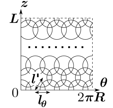
Figure 8: Schematic diagram of the configuration of wall particles in the ${{\theta}}$-${{z}}$ plane. Here, $R={a}+{{d}}/2$.

In Sec. II, we described the configuration of the wall particles as being nearly hexagonal. We first explain what “nearly hexagonal” means. Figure 8 shows a schematic diagram of the positions of wall particles in the ${{\theta}}$-${{z}}$ plane. Here the particles form a nearly hexagonal lattice with lattice constant $l_{{\theta}}$ in the ${{\theta}}$-direction and lattice constant $l^{\prime}$ in oblique directions. The configuration is perfectly hexagonal if $l_{{\theta}}=l^{\prime}$. In our simulation setup, however, we set $l_{{\theta}}\neq l^{\prime}$, and we consider this configuration to be nearly hexagonal. This is because of the periodicity in the ${{\theta}}$- and ${{z}}$-directions; if the configuration was perfectly hexagonal, the tube length $L$ and average tube radius $a$ would satisfy the relation $2\pi({a}+{{d}}/2)/n={L}/\sqrt{3}\,n^{\prime}$ for $n,n^{\prime}\in\mathbb{N}$. To avoid imposing this constraint, we consider the above nearly hexagonal lattice in this paper.

We introduce a parameter $l$ to determine the lattice constants $l_{{\theta}}\simeq l$ and $l^{\prime}\simeq l$. We denote the number of particles in a layer (particles with identical ${{z}}$ values) as $N^{\prime}_{\mathrm{w}}$ and define the number of layers $N_{\mathrm{l}}={N_{\mathrm{w}}}/N^{\prime}_{\mathrm{w}}$ as

$$N^{\prime}_{\mathrm{w}} =\biggl{\lfloor}\dfrac{2\pi({a}+{{d}}/2)}{l}\biggr{\rfloor},$$ (15)

$$N_{\mathrm{l}} =2\Biggl{\lfloor}\dfrac{L}{\sqrt{3}\,l}\Biggr{\rfloor},$$ (16)

where $\lfloor x\rfloor\equiv\max\{n\in\mathbb{N}|n\leq x\}$ is the integer part of $x$. From Eqs. (15) and (16), $l_{{\theta}}$ and $l^{\prime}$ are given as

$$l_{{\theta}} =\dfrac{2\pi({a}+{{d}}/2)}{N^{\prime}_{\mathrm{w}}}$$ (17)

$$l^{\prime} =\dfrac{2\sqrt{3}}{3}\dfrac{{L}}{N_{\mathrm{l}}}.$$ (18)

References

- Jaffrin and Shapiro (1971) M. Y. Jaffrin and A. H. Shapiro, Ann. Rev. Fluid Mech. 3, 13 (1971).
- Burns and Parkes (1967) J. C. Burns and T. Parkes, J. Fluid Mech. 29, 731 (1967).
- Shapiro et al. (1969) A. H. Shapiro, M. Y. Jaffrin, and S. L. Weinberg, J. Fluid Mech. 37, 799 (1969).
- Li (1970) C.-H. Li, J. Biomech. 3, 513 (1970).
- Yin and Fung (1971) F. C. P. Yin and Y. C. Fung, J. Fluid Mech. 47, 93 (1971).
- Weinberg et al. (1971) S. L. Weinberg, E. C. Eckstein, and A. H. Shapiro, J. Fluid Mech. 49, 461 (1971).
- Srinivasacharya et al. (2003) D. Srinivasacharya, M. Mishra, and A. R. Rao, Acta Mech. 161, 165 (2003).
- Hung and Brown (1976) T.-K. Hung and T. D. Brown, J. Fluid Mech. 73, 77 (1976).
- Fauci (1992) L. J. Fauci, Comput. Fluids 21, 583 (1992).
- Jiménez-Lozano et al. (2009) J. Jiménez-Lozano, M. Sen, and P. F. Dunn, Phys. Rev. E 79, 041901 (2009).
- Jiménez-Lozano and Sen (2010) J. Jiménez-Lozano and M. Sen, Phys. Fluids 22, 043303 (2010).
- Helbing (2001) D. Helbing, Rev. Mod. Phys. 73, 1067 (2001).
- Nakajima and Hayakawa (2009) C. Nakajima and H. Hayakawa, Prog. Theor. Phys. 122, 1377 (2009).
- Le Pennec et al. (1996) T. Le Pennec, K. J. Måløy, A. Hansen, M. Ammi, D. Bideau, and X.-l. Wu, Phys. Rev. E 53, 2257 (1996).
- Longhi et al. (2002) E. Longhi, N. Easwar, and N. Menon, Phys. Rev. Lett. 89, 045501 (2002).
- Beverloo et al. (1961) W. A. Beverloo, H. A. Leniger, and J. van de Velde, Chem. Eng. Sci. 15, 260 (1961).
- Nedderman et al. (1982) R. M. Nedderman, U. Tüzün, S. B. Savage, and G. T. Houlsby, Chem. Eng. Sci. 37, 1597 (1982).
- Mankoc et al. (2007) C. Mankoc, A. Janda, R. Arévalo, J. Pastor, I. Zuriguel, A. Garcimartín, and D. Maza, Granular Matter 9, 407 (2007).
- De-Song et al. (2003) B. De-Song, Z. Xun-Sheng, X. Guang-Lei, P. Zheng-Quan, T. Xiao-Wei, and L. Kun-Quan, Phys. Rev. E 67, 062301 (2003).
- Aguirre et al. (2010) M. A. Aguirre, J. G. Grande, A. Calvo, L. A. Pugnaloni, and J.-C. Géminard, Phys. Rev. Lett. 104, 238002 (2010).
- Hou et al. (2003) M. Hou, W. Chen, T. Zhang, K. Lu, and C. K. Chan, Phys. Rev. Lett. 91, 204301 (2003).
- Zhong et al. (2006) J. Zhong, M. Hou, Q. Shi, and K. Lu, J. Phys.: Condens. Matter 18, 2789 (2006).
- Huang et al. (2006) D. Huang, G. Sun, and K. Lu, Phys. Rev. E 74, 061306 (2006).
- Janda et al. (2009) A. Janda, R. Harich, I. Zuriguel, D. Maza, P. Cixous, and A. Garcimartín, Phys. Rev. E 79, 031302 (2009).
- To et al. (2001) K. To, P.-Y. Lai, and H. K. Pak, Phys. Rev. Lett. 86, 71 (2001).
- To (2005) K. To, Phys. Rev. E 71, 060301 (2005).
- Zuriguel et al. (2003) I. Zuriguel, L. A. Pugnaloni, A. Garcimartín, and D. Maza, Phys. Rev. E 68, 030301 (2003).
- Zuriguel et al. (2005) I. Zuriguel, A. Garcimartín, D. Maza, L. A. Pugnaloni, and J. M. Pastor, Phys. Rev. E 71, 051303 (2005).
- Janda et al. (2008) A. Janda, I. Zuriguel, A. Garcimartín, L. A. Pugnaloni, and D. Maza, Europhys. Lett. 84, 44002 (2008).
- O’Hern et al. (2002) C. S. O’Hern, S. A. Langer, A. J. Liu, and S. R. Nagel, Phys. Rev. Lett. 88, 075507 (2002).
- O’Hern et al. (2003) C. S. O’Hern, L. E. Silbert, A. J. Liu, and S. R. Nagel, Phys. Rev. E 68, 011306 (2003).
- Dauchot et al. (2005) O. Dauchot, G. Marty, and G. Biroli, Phys. Rev. Lett. 95, 265701 (2005).
- Olsson and Teitel (2007) P. Olsson and S. Teitel, Phys. Rev. Lett. 99, 178001 (2007).
- Hatano (2008) T. Hatano, J. Phys. Soc. Jpn. 77, 123002 (2008).
- Otsuki and Hayakawa (2009a) M. Otsuki and H. Hayakawa, Prog. Theor. Phys. 121, 647 (2009a).
- Otsuki and Hayakawa (2009b) M. Otsuki and H. Hayakawa, Phys. Rev. E 80, 011308 (2009b).
- Otsuki et al. (2010) M. Otsuki, H. Hayakawa, and S. Luding, Prog. Theor. Phys. Suppl. 184, 110 (2010).
- Evans and Morriss (1990) D. J. Evans and G. P. Morriss, Statistical Mechanics of Nonequilibrium Liquids (Academic Press, London, 1990).
- Binder (1973) K. Binder, Phys. Rev. B 8, 3423 (1973).
- Kob and Andersen (1994) W. Kob and H. C. Andersen, Phys. Rev. Lett. 73, 1376 (1994).
- Kob and Andersen (1995) W. Kob and H. C. Andersen, Phys. Rev. E 52, 4134 (1995).
- Binder (1987) K. Binder, Rep. Prog. Phys. 50, 783 (1987).
- Krzakala and Zdeborova (2011a) F. Krzakala and L. Zdeborova, J. Chem. Phys. 134, 034512 (2011a).
- Krzakala and Zdeborova (2011b) F. Krzakala and L. Zdeborova, J. Chem. Phys. 134, 034513 (2011b).
- Miyama and Sasa (2011) M. J. Miyama and S. Sasa, Phys. Rev. E 83, 020401 (2011).
- Jaffrin (1973) M. Y. Jaffrin, Int. J. Eng. Sci. 11, 681 (1973).
- Aarts and Ooms (1998) A. C. T. Aarts and G. Ooms, J. Eng. Math. 34, 435 (1998).
- Felderhof (2011) B. U. Felderhof, Phys. Rev. E 83, 036315 (2011).
- Brilliantov and Pöschel (2004) N. V. Brilliantov and T. Pöschel, Kinetic Theory of Granular Gases (Oxford University Press, Oxford, 2004).