Fisher information matrix for three-parameterexponentiated-Weibull distribution under type II censoring

Abstract

This paper considers the three-parameter exponentiated Weibull family under type II censoring. It first graphically illustrates the shape property of the hazard function. Then, it proposes a simple algorithm for computing the maximum likelihood estimator and derives the Fisher information matrix. The latter one is represented through a single integral in terms of hazard function, hence it solves the problem of computation difficulty in constructing inference for the maximum likelihood estimator. Real data analysis is conducted to illustrate the effect of censoring rate on the maximum likelihood estimation.

Keywords: Exponentiated Weibull Distribution; Hazard Function; Type II censoring; Maximum Likelihood Estimator; Fisher Information Matrix.

1 Introduction

In testing the reliability of a component, $n$ identical components are placed on life-testing. The type II censoring scheme is to stop the test procedure when one observes the $r$th failure, $r\leq n$. Various models have been proposed for lifetime distribution. Among those lifetime distributions, Weibull distribution is the most popular used. Based on Weibull distribution, various generalizations have been studied (Pham and Lai, 2007). Among those generalizations, one of the families is called exponentiated Weibull distribution (EWD), initially proposed by Mudholkar and Srivastava (1993). EWD family not only covers the one-parameter exponential family, exponentiated exponential family as a sub-family, but also covers the most popular used two-parameter Weibull family as a special sub-family. One of the nice features of EWD family is that it allows non-monotonic hazard functions, such as unimodal shaped and bathtub shaped, appeared in science, engineering and medical fields. For more shapes of hazard functions, see Mudholkar and Srivastava (1993). Mudholkar, Srivastava and Freimer (1995) reanalyzed the bus-motor-failure rate data using EWD family.

Singh, Gupta and Upadhyay (2002, 2005) studied the point estimators of three-parameters for EWD under complete data and type II censored using various estimation methods such as maximum likelihood method, Bayes method and generalized maximum likelihood method. Numerical comparisons were obtained for the point estimators. Ortega, Cancho and Bolfarine (2006) gave an influence diagnostics in exponentiated Weibull with censored data. Ortega, et al. (2006) states that “it is not possible to compute the Fisher information matrix…”.

In this paper, we derive a simple expression for the Fisher information matrix through a single integral of the hazard function, hence obtain the asymptotic normality of the maximum likelihood estimator of the three unknown parameters for EWD under type II censoring.

2 Shape property of the hazard function

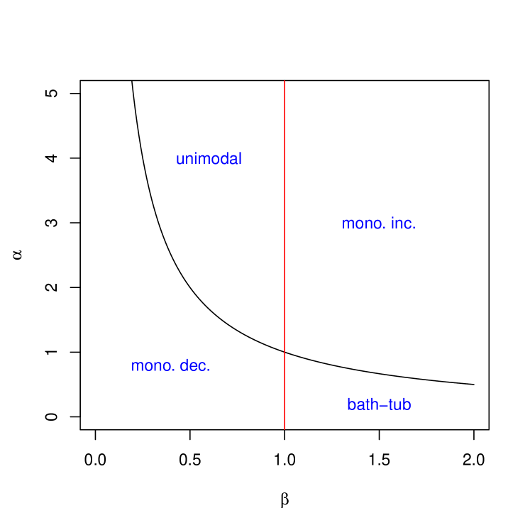
Figure 1: The graphical display of the four regions which separate the parameter domain for shape properties of the hazard function, where the curve is for $\alpha\beta=1$. mono. dec=monotonic decreasing, mono. inc.=monotonic increasing.

Assume that all $n$ independent components under testing have cumulative distribution function $F(x;\theta)$, density function $f(x;\theta)$ and hazard function $h(x;\theta)$ with parameter vector $\theta\in\Theta\subset R_{+}^{3}$, where $\Theta$ is an open set in $R_{+}^{3}$, $R_{+}=(0,\infty)$. Let $\theta=(\alpha,\beta,\sigma)^{T}$. Then the distribution and density functions are

$$F(x;\theta)=\left[1-e^{-\left({x\over\sigma}\right)^{\beta}}\right]^{\alpha},\ \ \ x>0$$

and

$$f(x;\theta)={\alpha\beta\over\sigma}\left({x\over\sigma}\right)^{\beta-1}e^{-\left({x\over\sigma}\right)^{\beta}}\left[1-e^{-\left({x\over\sigma}\right)^{\beta}}\right]^{\alpha},\ \ \ x>0$$

respectively. Here $\alpha$ and $\beta$ are shape parameters and $\sigma$ is a scale parameter. Notice that if $\alpha=1$, it reduces to the two-parameter Weibull distribution family. If $\beta=1$, it reduces to the exponentiated exponential family. If $\alpha=1$ and $\beta=1$, it is the one-parameter exponential family. If $\alpha=1$ and $\beta=2$, it reduces to Rayleigh distribution and generalized Rayleigh or Burr type X distribution if $\beta=2$.

The hazard function is the ratio of $f$ and $1-F$. It takes various shapes. To be more precise, the hazard function of EWD is

$$h(x)={{\alpha\beta\over\sigma}\left[1-\exp\left(-\left({x\over\sigma}\right)^{\beta}\right)\right]^{\alpha-1}\exp\left(-\left({x\over\sigma}\right)^{\beta}\right)\left({x\over\sigma}\right)^{\beta-1}\over 1-\left(1-\exp\left(-\left({x\over\sigma}\right)^{\beta}\right)\right)^{\alpha}}.$$ (1)

Mudholkar, Srivastava and Freimer (1995) stated that the monotonicity property of the hazard function is completely determined by $(\alpha,\beta)$ in the first quadrant. The first quadrant is divided into four regions as shown in Figure 1, where the curves are the boundaries of the four regions. That is $\alpha\beta=1$ and $\beta=1$. It is easy to understand that the shape property of the hazard function is independent of the scale parameter $\sigma$. To see this, let $X$ be EWD with parameters $\theta$, denoted by $X\sim EWD(\alpha,\beta,\sigma)$. Then $X/\sigma\sim EWD(\alpha,\beta,1)$. However the shape property with respect to the shape parameters is not easy to see. Mudholkar, Srivastava and Freimer (1995) gave the theorem (their Theorem 2.1), but no detail proof. We will illustrate the theorem through visualizing the sign of the derivative of the hazard function. For this purpose, we first derive the derivative function of the hazard function, then make comments on the sign of the derivative function.

Proposition 2.1

Let

$$s(z)=\beta z\ln z\left[(z-1)^{\alpha}+(\alpha-z)z^{\alpha-1}\right]+(\beta-1)(z-1)\left[z^{\alpha}-(z-1)^{\alpha}\right].$$

Then the sign of the derivative of the hazard function $h$ is the same as the function $s$.

Proof: Let $z=\exp\left(\left({x\over\sigma}\right)^{\beta}\right)$. Then $z>1$, $\ln z=\left({x\over\sigma}\right)^{\beta}$ and $x=\sigma\left(\ln z\right)^{1\over\beta}$. Rewrite $h$ function into a function in $z$ and denote as $r(z)$. We have, for $z>1$,

$$r(z)=h(\sigma\left(\ln z\right)^{1\over\beta})={\alpha\beta\left[1-z^{-1}\right]^{\alpha-1}z^{-1}\left(\ln z\right)^{\beta-1\over\beta}\over\sigma\left[1-(1-z^{-1})^{\alpha}\right]}={\alpha\beta\over\sigma}{(z-1)^{\alpha-1}\left(\ln z\right)^{\beta-1\over\beta}\over\left[z^{\alpha}-(z-1)^{\alpha}\right]}.$$

Thus, taking logarithm both sides, we have

$$\ln r(z)=\ln{\alpha\beta\over\sigma}+(\alpha-1)\ln(z-1)+{\beta-1\over\beta}\ln\ln z-\ln[z^{\alpha}-(z-1)^{\alpha}].$$

Taking derivative, we obtain

$${r^{\prime}(z)\over r(z)} = {\alpha-1\over z-1}+{\beta-1\over\beta}{1\over z\ln z}-{\alpha(z^{\alpha-1}-(z-1)^{\alpha-1})\over z^{\alpha}-(z-1)^{\alpha}}$$

$$= {\beta(\alpha-1)z\ln z+(\beta-1)(z-1)\over\beta z(z-1)\ln z}-{\alpha(z^{\alpha-1}-(z-1)^{\alpha-1}\over z^{\alpha}-(z-1)^{\alpha}}$$

$$= {\beta z\ln z\left[(z-1)^{\alpha}+(\alpha-z)z^{\alpha-1}\right]+(\beta-1)(z-1)\left[z^{\alpha}-(z-1)^{\alpha}\right]\over\beta z(z-1)\ln z\left[z^{\alpha}-(z-1)^{\alpha}\right]}$$

$$= {s(z)\over\beta z(z-1)\ln z\left[z^{\alpha}-(z-1)^{\alpha}\right]}$$

Hence the sign of $r^{\prime}(z)$ is the same as the sign of $s(z)$ since $r(z)>0$ and $\beta z(z-1)\ln z\left[z^{\alpha}-(z-1)^{\alpha}\right]>0$.

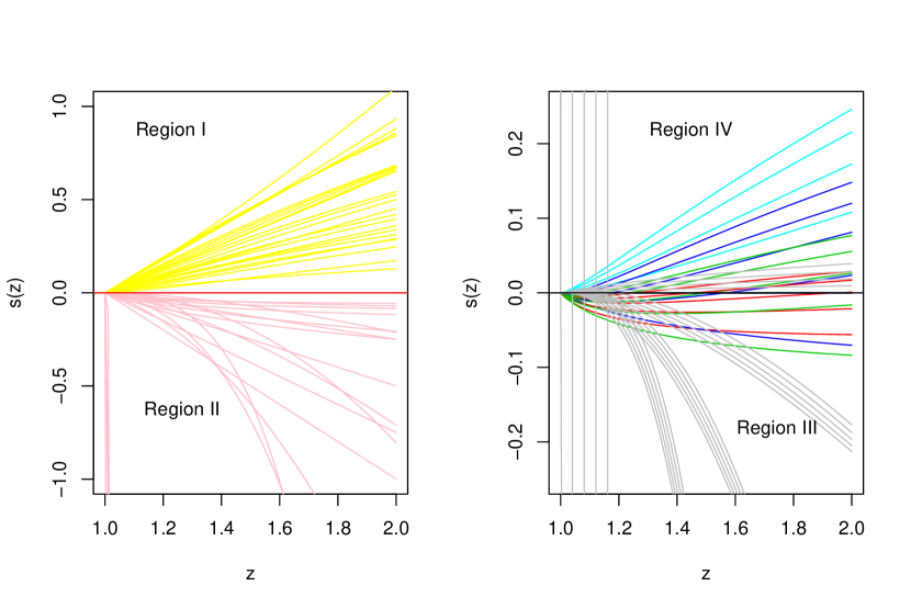
Figure 2: The graphs of $s(z)$ for the four defined regions. Region I=$\{(\alpha,\beta):\beta\geq 1\mbox{ and }\alpha\beta\geq 1\}$, region II=$\{(\alpha,\beta):\beta\leq 1\mbox{ and }\alpha\beta\leq 1\}$, region III=$\{(\alpha,\beta):\beta<1\mbox{ and }\alpha\beta<1\}$ and region IV=$\{(\alpha,\beta):\beta>1\mbox{ and }\alpha\beta<1\}$, respectively.

Figure 2 shows the graphs of $s(z)$ for parameters in the four regions. From the left panel, one observes that $s(z)$ takes pure positive and pure negative values in region I and region II, respectively, which implies that the hazard function is monotone increasing in region I and monotone decreasing in region II. From the right panel, one observes that $s(z)$ takes positive values first then drop to negative values in region III, which indicates the unimodal property of the hazard function. In region IV, it is shown that $s(z)$ takes negative values first then positive values indicating bath-tub shaped of the hazard function. Furthermore, one notices that in region IV, the function $s(z)$ may be positive or negative for all $z$ for some of the parameters $(\alpha,\beta)$. Overall, the shape of the hazard function is independent of the scale parameter.

3 Maximum likelihood estimator under type II censoring

Let $x_{1},...,x_{n}$ be the lifetimes of the $n$ independent components under testing. With type II censoring scheme, one observes the first $r$ order statistics, $x_{1:n}\leq x_{2:n}\leq\cdots\leq x_{r:n}$, of the sample $x_{1},...,x_{n}$. Based on the censored data $x_{1:n},...,x_{r:n}$, the likelihood function is

$$L(\theta)={n!\over(n-r)!}\prod_{i=1}^{r}f(x_{i:n};\theta)\left[1-F(x_{r:n};\theta)\right]^{n-r},\ \ x_{1:n}\leq x_{2:n}\leq\cdots\leq x_{r:n}.$$

The maximum likelihood estimator of $\theta$ satisfies the following score equations:

$${\partial\over\partial\theta}lnL(\theta) = \sum_{i=1}^{r}{{\partial\over\partial\theta}f(x_{i:n};\theta)\over f(x_{i:n};\theta)}-(n-r){{\partial\over\partial\theta}F(x_{r:n};\theta)\over 1-F(x_{r:n};\theta)}=0,$$

where ${\partial\over\partial\theta}f(x;\theta)=(f^{\prime}_{\alpha}(x;\theta),f^{\prime}_{\beta}(x;\theta),f^{\prime}_{\sigma}(x;\theta))^{T}$ and ${\partial\over\partial\theta}F(x;\theta)=(F^{\prime}_{\alpha}(x;\theta),F^{\prime}_{\beta}(x;\theta),F^{\prime}_{\sigma}(x;\theta))^{T}$. After some algebraic manipulations, we have

$${f^{\prime}_{\alpha}(x;\theta)\over f(x;\theta)} = {1\over\alpha}\left[1+\ln F(x;\theta)\right],$$ (2)

$${F^{\prime}_{\alpha}(x;\theta)\over 1-F(x;\theta)} = {1\over\alpha}{F(x;\theta)\ln F(x;\theta)\over 1-F(x;\theta)};$$ (3)

$${f^{\prime}_{\beta}(x;\theta)\over f(x;\theta)} = {1\over\beta}\left\{1+\log\left({x\over\sigma}\right)^{\beta}\left[1-\left({x\over\sigma}\right)^{\beta}+{(\alpha-1)xf(x;\theta)\over\alpha\beta F(x;\theta)}\right]\right\},$$ (4)

$${F^{\prime}_{\beta}(x;\theta)\over 1-F(x;\theta)} = {1\over\beta^{2}}\log\left({x\over\sigma}\right)^{\beta}{xf(x;\theta)\over 1-F(x;\theta)};$$ (5)

$${f^{\prime}_{\sigma}(x;\theta)\over f(x;\theta)} = -{\beta\over\sigma}\left[1-\left({x\over\sigma}\right)^{\beta}+{(\alpha-1)xf(x;\theta)\over\alpha\beta F(x;\theta)}\right],$$ (6)

$${F^{\prime}_{\sigma}(x;\theta)\over 1-F(x;\theta)} = {1\over\sigma}{xf(x;\theta)\over 1-F(x;\theta)}.$$ (7)

Notice that if $\{x_{i}\}$ is a random sample from EWD with parameter vector $\theta$, then $\{y_{i}=x_{i}^{\beta}\}$ is a random sample from exponentiated exponential distributed (EED) with shape parameter $\alpha$ and scale parameter $\lambda=\sigma^{\beta}$. Since $\beta>0$, $x_{1:n}\leq x_{2:n}\leq\cdots\leq x_{r:n}$ is equivalent to $y_{1:n}\leq y_{2:n}\leq\cdots\leq y_{r:n}$, the first $r$ order statistics of $y_{1},\cdots,y_{n}$.

Hence we propose the following back fitting algorithm to obtain the MLE of $\theta$:

• For a given initial value $\beta^{(0)}$ of $\beta$, maximize $L(\alpha,\beta^{(0)},\sigma)$ with respect to $(\alpha,\sigma)^{T}\in R_{+}^{2}$. Denote the maximizer by $(\alpha^{(1)},\sigma^{(1)})^{T}$.

• Substitute $\alpha=\alpha^{(1)},\sigma=\sigma^{(1)}$ into $L(\alpha,\beta,\sigma)$ to get profile likelihood function $L_{1}(\beta)$. Maximize $L_{1}(\beta)$ over $R_{+}$ to obtain $\beta^{(1)}$.

• Repeat Steps 1 and 2 $k$ times to get $\theta^{(k)}=(\alpha^{(k)},\beta^{(k)},\sigma^{(k)})^{T}$.

• Stop if $\|\theta^{(k)}-\theta^{(k-1)}\|<\epsilon$ for a pre-chosen small $\epsilon>0$.

THEOREM 3.1

The limit of the back fitting estimator is the MLE. That is,

$$\max_{\beta\in R_{+}}\max_{(\alpha,\sigma)^{T}\in R_{+}^{2}}L(\alpha,\beta,\sigma)=\max_{\theta\in R_{+}^{3}}L(\theta).$$ (8)

Proof: Denote the MLE of $\theta$ by $\hat{\theta}_{MLE}=(\hat{\alpha}_{MLE},\hat{\beta}_{MLE},\hat{\sigma}_{MLE})^{T}$ and the estimator obtained by back fitting algorithm by $\hat{\theta}_{BF}$.

It is clear that the right hand side of the equation (8) is bigger than or equal to the left hand side. For the other direction, one notices by definition that

$$\max_{\theta\in R_{+}^{3}}L(\theta) = L(\hat{\theta}_{MLE})\leq\max_{(\alpha,\sigma)^{T}\in R_{+}^{2}}L(\alpha,\hat{\beta}_{MLE},\sigma)$$

$$= L(\hat{\alpha}_{BF},\hat{\beta}_{MLE},\hat{\sigma}_{BF})\leq L(\hat{\alpha}_{BF},\hat{\beta}_{BF},\hat{\sigma}_{BF})$$

$$= \max_{\beta\in R_{+}}\max_{(\alpha,\sigma)^{T}\in R_{+}^{2}}L(\alpha,\beta,\sigma).$$

This completes the proof.

Hence for a given $\beta>0$, the problem is equivalent to find the MLE for EED with type II censored data $y_{1:n}=x_{1:n}^{\beta},\cdots,y_{r:n}=x_{r:n}^{\beta}$. In fact, the MLE of the EED parameters satisfies the following fix point equation

$$(\alpha,\lambda)=rg(\alpha,\lambda),$$ (9)

where $g(\alpha,\lambda)=(g_{1}^{-1}(\alpha,\lambda),g_{2}(\alpha,\lambda)$ and

$$g_{1}(\alpha,\lambda) = (n-r){\left(1-e^{-y_{r:n}/\lambda}\right)^{\alpha}\ln(1-e^{-y_{r:n}/\lambda})\over 1-\left(1-e^{-y_{r:n}/\lambda}\right)^{\alpha}}-\sum_{i=1}^{r}\ln\left(1-e^{-y_{i:n}/\lambda}\right),$$

$$g_{2}(\alpha,\lambda) = \left[(n-r){\alpha y_{r:n}e^{-y_{r:n}/\lambda}\left(1-e^{-y_{r:n}/\lambda}\right)^{\alpha-1}\over 1-\left(1-e^{-y_{r:n}/\lambda}\right)^{\alpha}}+(\alpha-1)\sum_{i=1}^{r}{y_{i:n}e^{-y_{i:n}/\lambda}\over 1-e^{-y_{i:n}/\lambda}}+\sum_{i=1}^{r}y_{i:n}\right]/r^{2}.$$

To solve equation (9), one can choose an initial value $\alpha^{(0)}$ and $\lambda^{(0)}$ for $\alpha$ and $\lambda$, respectively. Substitute $\alpha^{(0)}$ and $\lambda^{(0)}$ into the right hand side of the equation (9) to get $\alpha^{(1)}$ and $\lambda^{(1)}$. Continue this procedure $k$ times to get $\alpha^{(k)}=rg_{1}^{-1}(\alpha^{(k-1)},\sigma^{(k-1)})$ and $\sigma^{(k)}=rg_{2}^{-1}(\alpha^{(k-1)},\lambda^{(k-1)})$ for $k=0,1,...$. The iteration stops when $\|(\alpha^{(k)},\lambda^{(k)})-(\alpha^{(k-1)},\lambda^{(k-1)})\|<\epsilon$, a given pre-selected small positive number such as $10^{-8}$. For given $\beta$, the estimator of $(\alpha,\lambda)$ is denoted by $(\hat{\alpha},\hat{\lambda})$, hence the estimator of $\sigma$ is a function of $\beta$, denoted by $\hat{\sigma}(\beta)=\hat{\lambda}^{1/\beta}$. Plug in the $\hat{\alpha}$ and $\hat{\sigma}(\beta)$ into the log-likelihood function to obtain the profile likelihood function $L_{1}(\beta)$ in $\beta$. Maximizing $L_{1}(\beta)$ to obtain $\hat{\beta}$ and hence to obtain the maximum likelihood estimator $\hat{\theta}=(\hat{\alpha},\hat{\beta},\hat{\sigma})^{T}=(\hat{\alpha},\hat{\beta},\hat{\sigma}(\hat{\beta}))^{T}$.

4 Fisher information matrix

Now we assume that $r/n\rightarrow p\in(0,1)$ as $n\rightarrow\infty$. Notice that the hazard function $h(x;\theta)=f(x,\theta)/(1-F(x;\theta))$. Denote the Fisher information matrix based on the first $r$ order statistics by $I_{p}(\theta)$ and let $\lambda_{p}$ be the $100p$ percentile of $F(x;\theta)$ such that $F(\lambda_{p};\theta)=p$.

Lemma 4.1

(Zheng, 2001) Assume $F(x;\theta)$ has the same support for any $\theta\in\Theta$, an open set in $R^{k}$. For $x\in R$ and $\theta\in\Theta$, assume

$${\partial\over\partial\theta}f(x;\theta)={\partial^{2}\over\partial\theta\partial x}F(x;\theta)={\partial^{2}\over\partial x\partial\theta}F(x;\theta),$$

where all derivatives exist. Furthermore, under the interchangeability property for orders of limits, derivative and integral, the limiting Fisher information matrix can be expressed as a single integral of hazard function under type II censoring. That is,

$$I_{p}(\theta)=\int_{0}^{\lambda_{p}}\left[{\partial\over\partial\theta}\log h(x;\theta)\right]\left[{\partial\over\partial\theta}\log h(x;\theta)\right]^{T}f(x;\theta)\ dx.$$

Consequently, the asymptotic covariance matrix of the maximum likelihood estimator of $\theta$ based on the first $r$ order statistics is $I_{p}^{-1}(\theta)$.

Notice that

$${\partial\over\partial\theta}\log h(x;\theta)={{\partial\over\partial\theta}f(x;\theta)\over f(x;\theta)}+{{\partial\over\partial\theta}F(x;\theta)\over 1-F(x;\theta)}.$$ (10)

Thus, for EWD family, the equations (2)-(7) imply that

$${\partial\over\partial\alpha}\ln h(x;\theta) = {1\over\alpha}\left[1+{\ln F(x;\theta)\over 1-F(x;\theta)}\right],$$ (11)

$${\partial\over\partial\beta}\ln h(x;\theta) = {1\over\beta}\left\{1+\ln\left({x\over\sigma}\right)^{\beta}\left[1-\left({x\over\sigma}\right)^{\beta}+{(\alpha-1)xf(x;\theta)\over\alpha\beta F(x;\theta)}+{xf(x;\theta)\over\beta(1-F(x;\theta))}\right]\right\},$$ (12)

$${\partial\over\partial\sigma}\ln h(x;\theta) = -{\beta\over\sigma}\left\{1-\left({x\over\sigma}\right)^{\beta}+{(\alpha-1)xf(x;\theta)\over\alpha\beta F(x;\theta)}+{xf(x;\theta)\over\beta(1-F(x;\theta))}\right\}.$$ (13)

Denote the Fisher information matrix based on the first $r$ order statistics by

$$I_{p}(\theta)=\left[I_{p}^{ij}(\theta)\right],i=1,2,3;j=1,2,3.$$

Let

$$\psi(z;\alpha)=1+\ln(1-z)\left[1+\left({1-z\over z}\right)\left(1-{\alpha\over 1-z^{\alpha}}\right)\right].$$

Notice that $\psi(z;1)=1$. Then, we have our main theorem.

THEOREM 4.1

Let $r/n\rightarrow p=F(\lambda_{p};\theta)\in(0,1)$. For EWD family with parameter vector $\theta=(\alpha,\beta,\sigma)^{T}$ under type II censoring, we have

$$I_{p}^{11}(\theta) = {1\over\alpha^{2}}\int_{0}^{p}\left[1+{\ln x\over 1-x}\right]^{2}\ dx,$$ (14)

$$I_{p}^{22}(\theta) = {\alpha\over\beta^{2}}\int_{0}^{p^{1/\alpha}}\bigg{\{}1+\ln[-\ln(1-x)]\psi(x;\alpha)\bigg{\}}^{2}x^{\alpha-1}\ dx,$$ (15)

$$I^{33}(\theta) = \alpha\left({\beta\over\sigma}\right)^{2}\int_{0}^{p^{1/\alpha}}\psi^{2}(x;\alpha)x^{\alpha-1}\ dx,$$ (16)

$$I_{p}^{12}(\theta) = I_{p}^{21}(\theta)={\alpha\over\beta}\int_{0}^{p^{1/\alpha}}\left({1\over\alpha}+{\ln x\over 1-x^{\alpha}}\right)\bigg{\{}1+\ln[-\ln(1-x)]\psi(x;\alpha)\bigg{\}}x^{\alpha-1}\ dx,$$ (17)

$$I_{p}^{13}(\theta) = I_{p}^{31}(\theta)=-{\alpha\beta\over\sigma}\int_{0}^{p^{1/\alpha}}\left({1\over\alpha}+{\ln x\over 1-x^{\alpha}}\right)\psi(x;\alpha)x^{\alpha-1}\ dx,$$ (18)

$$I_{p}^{23}(\theta) = I_{p}^{32}(\theta)=-{\alpha\over\sigma}\int_{0}^{p^{1\over\alpha}}\left\{1+\ln[-\ln(1-x)]\psi(x;\alpha)\right\}\psi(x;\alpha)x^{\alpha-1}\ dx.$$ (19)

Proof: By Lemma 4.1, equations (11) and $F(\lambda_{p};\theta)=p$, we have

$$I_{p}^{11}(\theta) = \int_{0}^{\lambda_{p}}\left[{\partial\over\partial\alpha}\ln h(x;\theta)\right]^{2}\ dF(x;\theta)$$

$$= \int_{0}^{\lambda_{p}}{1\over\alpha}\left[1+{\ln F(x;\theta)\over 1-F(x;\theta)}\right]\ dF(x;\theta)$$

$$= {1\over\alpha^{2}}\int_{0}^{p}\left[1+{\ln x\over 1-x}\right]^{2}\ dx,$$

which completes the proof of equation (14). To proof (15), we introduce new variable by change of variables using $1-e^{-\left({x\over\sigma}\right)^{\beta}}=z$. Then $F(x;\theta)=z^{\alpha}$, $\left({x\over\sigma}\right)^{\beta}=-\ln(1-z)$, $f(x;\theta)dx=\alpha z^{\alpha-1}dz$,

$${xf(x;\theta)\over\alpha\beta F(x;\theta)}=-{(1-z)\ln(1-z)\over z},$$ (20)

$${xf(x;\theta)\over\beta(1-F(x;\theta))}=-{\alpha z^{\alpha-1}(1-z)\ln(1-z)\over 1-z^{\alpha}},$$ (21)

and

$$1-\left({x\over\sigma}\right)^{\beta}+{(\alpha-1)xf(x;\theta)\over\alpha\beta F(x;\theta)}+{xf(x;\theta)\over\beta(1-F(x;\theta))}=\psi(z;\alpha).$$ (22)

Equations (12) and (22) imply that

$$I_{p}^{22}(\theta) = \int_{0}^{\lambda_{p}}\left[{\partial\over\partial\beta}\ln h(x;\theta)\right]^{2}\ dF(x;\theta)$$

$$= {\alpha\over\beta^{2}}\int_{0}^{p^{1/\alpha}}\left[1+\ln(-\ln(1-x))\psi(x;\alpha)\right]^{2}x^{\alpha-1}\ dx,$$

which completes the proof of (15). Similarly, direct algebraic manipulations lead the other equations (16)-(19).

Using integration and Taylor series expansion methods, one can verify that EWD satisfies the regularity conditions (Bhattacharyya, 1985). Hence we have the asymptotic normality theorem.

THEOREM 4.2

Let $r/n\rightarrow p=F(\lambda_{p};\theta)\in(0,1)$. For EWD family with parameter vector $\theta=(\alpha,\beta,\sigma)^{T}\in\Theta$ under type II censoring, we have

$$\sqrt{n}\left(\hat{\theta}_{MLE}-\theta\right)\rightarrow N_{3}(0,I_{p}^{-1}(\theta)),\mbox{ as $n\rightarrow\infty$}.$$

5 Real data analysis: two examples

In this section, we use maximum likelihood method to fit two real data sets. One is the ball bearings lifetime analyzed in Gupta and Kundu (2001) and the other is the breaking stress of carbon fibres (in Gba) from Nichols and Padgett (2006). For the first data set, Caroni (2002) has pointed out that the data set contains censored points. For the second data, it will be interesting to see how the censoring rate affect the estimation. We consider three censoring rates of no censoring, 10% censoring and 20% censoring. The ball bearings lifetime data set contains 23 observations, while the breaking stress of carbon fibres data contains 100 observations. We fit the data sets using both the exponentiated exponential distribution (EED) and the exponentiated Weibull distribution (EWD). For the maximum likelihood estimates of EED, a modified quasi-Newton method with box constraints in the function optim() in R package is used. The maximum likelihood estimates are presented in Table 1. Note that $EED(\alpha,\sigma)=EWD(\alpha,1,\sigma)$.

Table 1: Maximum likelihood estimates of the model parameters

for ball bearings lifetime

		Censoring rate
Distribution	Estimate	$0\%$	$10\%$	$20\%$
EED	$\alpha$	5.2707	5.0752	5.0728
	$\sigma$	31.0035	31.7540	31.7592
	-log(likelihood)	112.9762	104.6143	91.0536
EWD	$\alpha$	4.7446	7.7412	9.0634
	$\beta$	1.0444	0.8462	0.7924
	$\sigma$	33.6008	22.3618	19.3368
	-log(likelihood)	112.9740	104.5917	91.0128

The maximum likelihood estimator is robust against various censoring rates for EED. On the other hand it is sensitive for EWD. The standard likelihood ratio test shows that the shape parameter $\beta$ in EWD is not significant different from one, hence the EED is suitable in modeling the ball bearings lifetime. The result is consistent with Gupta and Kundu (2001) for no censoring data. This property still holds under various censoring data. As an illustration, with 10% censoring rate, the log-likelihood function and its contour plot is given in Figure 3.

Table 2: Maximum likelihood estimates of the model parameters

for break stress data

		Censoring rate
Distribution	Estimate	$0\%$	$10\%$	$20\%$
EED	$\alpha$	7.7883	7.6053	6.9949
	$\sigma$	0.9870	.9994	1.0487
	-log(likelihood)	146.1823	137.4110	130.8363
EWD	$\alpha$	1.3169	.4432	.1840
	$\beta$	2.4091	5.5320	12.4404
	$\sigma$	2.6824	3.4164	3.6032
	-log(likelihood)	141.3320	130.5830	125.6935

Once again, the maximum likelihood estimator is robust against various censoring rates for EED. On the other hand it is sensitive for EWD. The shape parameter $\beta$ in EWD is significant different from one by the standard likelihood ratio test. Hence it is better to use EWD in modeling the break stress. The result is consistent with Nichols and Padgett (2006). The EWD fit still holds for censored data. As an illustration, with 10% censoring rate, the log-likelihood function and its contour plot is given in Figure 4.

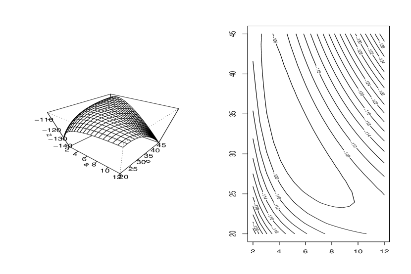
Figure 3: The log-likelihood function and its contour plot of EED under 10% censoring rate for ball bearings lifetime data.

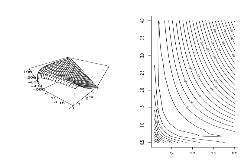
Figure 4: The log-likelihood function and its contour plot of EED under 10% censoring rate for the break stress data.

6 Conclusion

For data generated from exponentiated Weibull distribution, we visualize the shape of the hazard function under various shape and scale parameters. Under type II censoring, we propose a simple algorithm for computing the maximum likelihood estimator and derive the Fisher information matrix. The latter one is represented through a single integral in terms of hazard function, hence it solves the problem of computation difficulty in constructing inference for the maximum likelihood estimator. Data analysis for two real data sets shows that the maximum likelihood estimator is robust with respect to the censoring when the underlying distribution is the exponentiated exponential, but not for general exponentiated Weibull distribution when the shape parameter $\beta\neq 1$.

References

[1]
Balasooriya, U. and Balakrishnan, N. Reliability sampling plans
for log-normal distribution, based on progressively-censored
samples. IEEE Trans. Reliability, 49 (2000), 199-203.
[2] Banerjee A. and Kundu, D. Inference based on type-II
hybrid censored data from a Weibull distribution. IEEE Trans.
Reliability, 57 (2008) 2, 369-378.
[3] Bhattacharyya, G. K. The asymptotics of maximum likelihood and related estimators based on type II censored data. Journal of the American Statistical Association, 80 (1985), 398-404.
[4]
Caroni, C. The correct ”Ball Bearings” data. Lifetime data analysis, 8 (2002), 395-399.
[5]
Gupta, R. D. and Kundu, D. Expeonentiated exponential familty: an alternative to Gamma aand Weilbull distributions. Biomedical Journal, 43 (2001), 117-130.
[6]
Mudholkar, G. S. and Srivastava, D. K. Exponential Weibull family
for analyzing bathtub failure-rate data. IEEE Trans.
Reliability, 42 (1993), 299-302.
[7]
Mudholkar, G. S., Srivastava, D. K. and Freimer, M. The
exponentiated Weibull family: A reanalysis of the
Bus-motor-failure data. Technometrics, 37 (1995), 436-445.
[8]
Nichols, M. D. and Padgett, W. J. A bootstrap control chart for Weibull percentiles. Quality and reliability engineering international, 22 (2006), 141-151.
[9] Ortega, E. M.M., Cancho, V.G. and Bolfarine, H.
Influence diagonostics in exponentiated-Weibull regression models
with censored data. SORT, 30 (2006) 2, 171-192.
[10]
Pham, H. and Lai, C.-D. On recent generalizations of the Weibull
distribution. IEEE Trans. Reliability, 56 (2007), 454-458.
[11]
Singh, U., Gupta, P. K. and Upadhyay, S. K. Estimation of
exponentiated Weibull shape parameters under LINEX loss function.
Commun. Statist. Simulation Comput. , 31 (2002), 523-537.
[12]
Singh, U., Gupta, P. K. and Upadhyay, S. K. Estimation of
three-parameter exponentiated-Weibull distribution under type-II
censoring. J Stat Plan Inference, 134 (2005), 350-372.
[13]
Zheng, Gang. A characterization of the factorization of hazard
function by the Fisher information under type II censoring with
application to the Weibull family. Statist. Prob. Lett., 52
(2001), 249-253.