Finite energy spectral function of an anisotropic 2D system of coupled Hubbard chains

Abstract

We study the crossover from the one-dimensional to the two-dimensional Hubbard model in the photoemission spectra of weakly coupled chains. The chains with on-site repulsion are treated using the spin-charge factorized wave function, that is known to provide an essentially exact description of the chain in the strong coupling limit. The hoppings between the chains are considered as a perturbation. We calculate the dynamical spectral function at all energies in the random-phase approximation, by resuming an infinite set of diagrams. Even though the hoppings drive the system from a fractionalized Luttinger-liquid-like system to a Fermi-liquid-like system at low energies, significant characteristics of the one-dimensional system remain in the two-dimensional system. Furthermore, we find that introducing (frustrating) hoppings beyond the nearest neighbor one, the interference effects increase the energy and momentum range of the one–dimensional character.

I Introduction

The Hubbard model is believed to contain most of the fundamental physics of a great variety of materials ranging from weak interacting metals to Mott insulators. It may also capture some of the phenomena responsible for the high $T_{c}$ superconductivity of cuprates. In one spatial dimension the Hubbard chain is exactly solvable by the Bethe ansatz Lieb_1968 , furthermore, the low energy properties are understood in details within the Luttinger Liquid (LL) theory Haldane . In particular, the elementary excitations turn out to be fractionalized, carrying either charge or spin quantum numbers, a property that is a rather generic feature in 1D strongly interacting electron systems Book . Thanks to the advent of bosonization the low energy physics of 1D interacting electrons is now well understood including the computation of many observables Book ; Gogolin_1998 ; Voit ; Frahm ; CarmeloGS . However, despite the enormous success of these complementary approaches the computation of observables for arbitrary energies was obtained only in some restricted limits Penc_1995 ; Penc_1996 ; Halffilling or using some additional approximations Sing_2003 ; Carmelo_2004 ; Carmelo_2004_b ; Carmelo_2006 ; Bozi_2008 .

In higher dimensions the physical picture is much less clear. It has fueled controversy, mainly motivated by the hight Tc phenomena in the layered cuprate oxides. Generically, in dimensions higher than one, excitations are not fractionalized, the most well-known example being the quasi-particles in a Fermi liquid (FL). A few remarkable experimental and model examples exist, however, where the electrons fractionalize. The most spectacular example is the fractional quantum Hall effect, where fractionalization of quasiparticles has been predicted theoreticallyFQHEthe and consequently found experimentally FQHEexp . Fractionalization has also been theoretically proposed in electron systems with frustrated nearest neighbor interactions tVmodel . Further examples include quantum spin-liquids, where the presence of frustration may lead to deconfinement of the spinons in the two-dimensional systemSachdev1 . For example, the quasi-two dimensional triangular spin system Cs₂CuCl₄Coldea2d has an excitation spectrum that can be described, similarly to the one dimensional case Heisenberg , by a continuum originated from fractionalized pairs of spin $1/2$ spinonsKohno_2007 . This property has been verified experimentally for several quasi-one dimensional spin $1/2$ systems like CPC CPC , KCuF₃ Nagler ; Tennant and copper benzoate Dender .

Experimentally, the single–particle properties of the material are most directly measured by photoemission. The intensity of the extraction of the electron by photon at given energy and momentum transfer is directly proportional to the spectral function – the imaginary part of the one-particle Green’s function. If most of the spectral weight is carried by well defined spectral lines one expects excitations to be sharp, electron-like coherent modes (quasiparticles). On the contrary, broad continua signal fractionalization of the electronic degrees of freedom.

Low energy descriptions for the two dimensional case have been proposed that predict a fractionalization description of the low energy physics. Experimentally such low energy features are difficult to observe in the photo-emission data since they are obscured by resolution and noise. Therefore, it is useful to have a prediction over the full energy range to compare with experiments. The motivation for this work is twofold: on the one hand to provide an approximate spectral function valid to arbitrary energy and on the other to clarify the role of frustration in the underlying excitation.

In this work we address the dimensional crossover from one to two dimensions in a strongly correlated electron system by coupling Hubbard chains within the random phase approximation (RPA). This approximation leads to a description of the 2D quantities spectral function in terms of the 1D Greens’s function of the chain. Though coupled one-dimensional chain tend to order at low temperature, in this work we will assume that we are at sufficiently high energies $\omega$ and temperatures $T$ , typically larger than some crossover temperature $T_{\text{1D}}$ after which LL perturbation should be valid. The general expression obtained by the RPA for the two dimensional spectral function is valid for any values of $U$ and filling factor, as well as for any kind of small inter-chain hopping. In particular it is possible to study the role of hopping in different geometries, highly frustrated cases as well as non-frustrated ones. Due to the lack of theoretical expressions for the spectral function in one dimensional for generic $U$ we concentrate our study on the $U\to\infty$ limit using the results derived in Penc_1997 . The exact results obtained for the spectral function of the Hubbard chain in the $U\rightarrow\infty$ limit, can be extended to finite but large $U$ and are used in the RPA to obtain the same function in higher dimensions.

Previous works have dealt with the issue of coupled LL or coupled Hubbard chains. Contrasting with the LL-like features of decoupled chains, FL behavior is generically expected for weakly interacting systems and large inter-chain hopping terms. The interpolation between LL and FL regimes as the inter-chain hopping increases, as well as the energy scales for which each description is valid have been largely discussed.

Using perturbative renormalization group (RG) and an RPA-like expression for the two-dimensional Green’s function, it was shown Wen_1990 , starting from a LL, that the hopping is relevant if $\theta<1$ and irrelevant if $\theta>1$, where $\theta$ is the LL exponent characterizing the low frequency behavior of the density of states $N\left(\omega\right)\sim\left|\omega\right|^{\theta}$, (note that $\theta=0$ corresponds to the non-interacting case). In the first case the two-dimensional Green’s function develops well define poles near the Fermi energy with a nonzero quasiparticle residue $\left(Z\right)$ for non-vanishing inter-chain hoppings and in the second case $Z$ vanishes. In the same direction it was pointed out that using a $d=1+\epsilon$ expansion that the only weak-coupling fixed point for $\epsilon>0$ is the FL one Castellani_1994 . Using a path integral formulation Boies_1995 (like RPA) the results of Wen_1990 where rederived, but it was pointed out that higher order processes could extend the FL behavior beyond $\theta=1$. Subsequent works, using exact resummation of some infinite class of diagrams Arrigoni_1998 ; Arrigoni_1999 ; Arrigoni_2000 , also corroborate this result. It was also shown, using bosonization, that even if long range 3D Coulomb interactions were considered the 1D LL regime leads to a FL, for any hopping, but anomalous scaling was found in the FL phase for small hoppings Kopietz_1995 ; Kopietz_1997 .

The picture that FL behavior is obtained as soon as inter-chain hopping is introduced has, however, to be interpreted as being valid only above some finite energy scale. The introduction of inter-chain hoppings will in general lead to instabilities towards some possible ordered phases. The phase diagram of a system of coupled chains, including ordered phases, was studied in Refs. Balentsa ; Lin ; Wu ; Nickel_2005 ; Nickel_2006 , e.g. The FL behavior appears for energy scales higher then the critical temperatures of such ordered phases.

Moreover, for energies higher than some characteristic energy of the order of the inter-chain hopping amplitude (possibly renormalized by the interactions), one expects to recover LL features. Thus only for intermediate energies is the FL picture expected to hold. Indeed in Ref. Clarke it was argued that even though the transverse hopping is a relevant perturbation, in the RG sense, incoherent single particle hopping between chains can lead to a LL-like behavior. This was confirmed in Poilblanc ; Capponi using exact diagonalizations (ED) and quantum Monte Carlo (QMC) since the incoherent part of the spectral function (SF) is less affected by inter-chain hopping, and the Drude weight is small compared to the incoherent weight, even for small $\theta$. For larger $\theta$ the hopping between chains becomes fully incoherent. Furthermore, considering a higher dimensional mesh of coupled LL it was shown that there are mixed characteristics of LL and FL Guinea .

A rather unifying picture was obtained using chain dynamical mean-field theory (CDMFT)Biermann_2001a . These studies observe a crossover from a LL at high temperatures to a FL at low T with the coexistence of a Drude feature with small spectral weight and a large incoherent weight.

Several studies also treated the case of coupled Mott insulators. The RPA approximation was used in Essler and it was found that for high enough hopping and small enough Coulomb coupling the Mott-Hubbard gap closes and small Fermi pockets appear in the Fermi surface with a finite $Z$. However, it was shown using CDMFT that when the gap closes there is a continuous FS and no pockets Biermann_2001a . These results were also confirmed in Berthod but it was found that between the Mott phase and the FS phase there is an intermediate phase where there are pockets (arcs because of spectral weight inhomogeneities). Defining the FS both by the poles and zeros of the $\text{Re}G(\omega,\mathbf{k})$ it was shown that the Luttinger Theorem Dzyaloshinskii_2003 is satisfied.

The paper is structured as follows: In section II we discuss the model and method used, briefly reviewing the RPA approach. In section III we present results for the spectral function at low energies where a Luttinger-liquid-like universal description holds and compare the results with other methods previously obtained. In section IV we consider the regimes of finite energies and consider finite but large $U$ values, the infinite $U$ limit where the spins are dispersionless and the half-filing Mott-insulator case. In section V we study the role of frustration comparing a square, a triangular and a fully frustrated lattices. We present some conclusions in section VI. Also, in Appendix A we review the method of Ref. Kohno_2007 developed for the spin structure factor of the Heisenberg antiferromagnet in a triangular lattice and present its generalization to the electron spectral function. In Appendix B we briefly review the method used for the calculation of the spectral function for the Hubbard chain. In Appendix C we review the derivation of the RPA formulation and derive the expansion for its leading correction. This involves the knowledge of higher correlation functions for the Hubbard chain, which are not available at this time.

II Model and Method

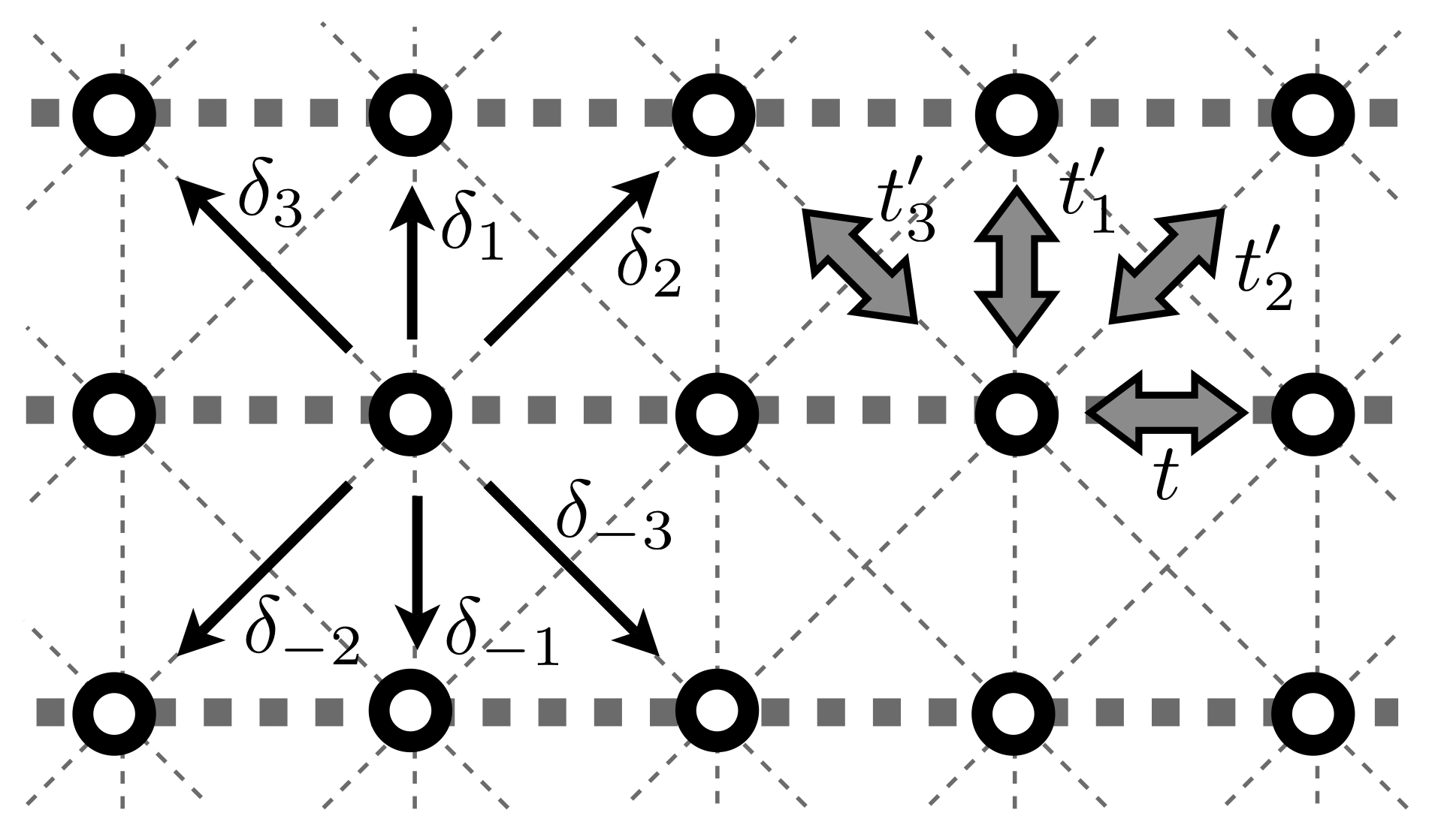
Figure 1: Direction of the hopping terms in the 2D Hubbard model.

This section presents the method used to obtain the spectral function of the weakly coupled Hubbard chains in terms of the one dimensional spectral function. In order to set the notation we write the Hamiltonian for the 2D Hubbard model as sum of an intra and an inter-chain term,

$$H = \sum_{y}H_{U,y}+H_{\perp},$$

here

$$H_{U,y} = \sum_{x,\sigma}-t\ \left[c_{x,y,\sigma}^{\dagger}c_{x+1,y,\sigma}+c_{x+1,y,\sigma}^{\dagger}c_{x,y,\sigma}\right]$$

$$+U\sum_{x,y}n_{x,y,\uparrow}n_{x,y,\downarrow}$$

is the intra-chain contribution to the Hamiltonian of a chain parallel to the $x$ direction and the subscript $y$ labels the direction perpendicular to the chains. The hopping amplitude between the sites in the chain is denoted by $t$, while $U$ is the usual on-site repulsion that penalizes doubly occupancy of a given site. The transverse term is given by

$$H_{\perp} =-\sum_{i}\sum_{\mathbf{r},\sigma}t^{\prime}_{i}\ \left(c_{\mathbf{r},\sigma}^{\dagger}c_{\mathbf{r}+\boldsymbol{\delta}_{i},\sigma}+c_{\mathbf{r}+\boldsymbol{\delta}_{i},\sigma}^{\dagger}c_{\mathbf{r},\sigma}\right)$$

where $t^{\prime}_{i}$ labels the different inter-chain hoppings along the directions $\boldsymbol{\delta}_{i}$ displayed in Fig.1. As shown, setting $t^{\prime}_{2}=t^{\prime}_{3}=0$ corresponds to an anisotropic square lattice, $t^{\prime}_{2}=t^{\prime}_{1}$ and $t^{\prime}_{3}=0$ to an anisotropic triangular lattice, and $t^{\prime}_{1}\neq 0$ and $t^{\prime}_{2}=t^{\prime}_{3}$ to the square lattice with diagonal hoppings.

II.1 RPA and spectral function

As briefly reviewed in Appendix C, the single electron Green’s function in the so called random phase approximation (RPA) is given by

$$G\left(\omega,\mathbf{k}\right) = \left[G_{1D}^{-1}\left(\omega,k_{x}\right)-t^{\prime}\left(\mathbf{k}\right)\right]^{-1}$$ (1)

where

$$t^{\prime}(\mathbf{k})=-2\sum_{i}t^{\prime}_{i}\cos\left(\mathbf{k}.\boldsymbol{\delta}_{i}\right)$$ (2)

$$=-2\left[t^{\prime}_{1}\cos\left(k_{y}\right)+t^{\prime}_{2}\cos\left(k_{y}+k_{x}\right)+t^{\prime}_{3}\cos\left(k_{y}-k_{x}\right)\right]$$

is the Fourier transform of the hopping matrix. Here $G_{1D}$ is the Green’s function of the one-dimensional system, assumed to be known. In this work it is calculated exactly. The Fermi momentum $\mathbf{k}_{F}$ and the QP weight are obtain from Eq. (1) requiring

$$G^{-1}\left(\omega=0,\mathbf{k}_{F}\right)=0$$ (3)

$$Z^{-1}=\partial_{\omega}G^{-1}\left(\omega=0,\mathbf{k}_{F}\right).$$ (4)

In several works pioneered by Wen Wen_1990 this expression has been used to study weakly coupled Luttinger Liquids Boies_1995 ; Tsvelik_1996 . Note that Eq. (1) is exact for non-interacting electrons $\left(\theta=0\right)$.

Using Eq. (1) and the asymptotic form of the retarded Green’s function, in the low energy limit given by bosonization and parameterized by

$$\theta=\frac{1}{4}\left(K_{c}+\frac{1}{K_{c}}-2\right)$$ (5)

where $K_{c}$ is the Luttinger parameter, it was shown Wen_1990 ; Boies_1995 ; Tsvelik_1996 ; Gogolin_1998 that for $\theta<1$ there is a nonvanishing QP weight

$$Z\sim\left(\frac{v_{s}}{v_{c}}\right)^{\gamma}\left|\frac{t^{\prime}\left(\mathbf{k}\right)}{\Lambda}\right|^{\frac{\theta}{1-\theta}}$$ (6)

for an arbitrary $t^{\prime}\neq 0$, where $\Lambda$ is an energy cutoff and $\gamma$ is a exponent that can be explicitly computed (see chap. 19 of Gogolin_1998 ). Note that for the non-interacting case $\theta=0$, the low energy regime of the infinite $U$ limit of the Hubbard model is recovered setting $\theta=1/8$ and higher values of $\theta$ correspond to models with long range interaction. Besides the region $\theta>1$, where no coherent mode is found at the RPA level in Tsvelik_1996 ; Gogolin_1998 , the authors considered the regimes $\theta<1/2$ and $\theta>1/2$ for which the exponent $\gamma$ in (6) changes from positive to negative. They concluded that the value of the QP residue will be larger in the second region. We will see further that there is a clear physical signature separating these two regimes.

As stated in the introduction $t^{\prime}$ is a relevant perturbation in the RG sense, and thus the above treatment is valid only for energies $T,\omega>T_{c}$ , where $T_{c}$ is the highest critical temperature of all the possible order phases towards which the system is unstable at low energy. Another energy scale is defined by $T_{1x}>T_{c}$ which separates a low energy regime where the pole of the Green’s functions is physically perceptible Boies_1995 from an higher energy regime for which fully coherent 2D hopping is suppressed. For the non-interacting case $\left(\theta=0\right)$ $T_{1x}$ is of the order of the interchain coupling $t^{\prime}$. It has been shown Boies_1995 that for the interacting case this energy scale is reduced yielding $T_{1x}\sim\Lambda\left(\frac{t^{\prime}}{\Lambda}\right)^{1/\left(1-\theta\right)}$ for $\theta<1$. For $\theta>1$ this treatment leads to a vanishing $T_{1x}$; however, as also noticed in Boies_1995 , higher order terms that consider two-particle processes define another energy scale $T_{2x}$ that will overtake $T_{1x}$ and further extend beyond $\theta=1$ the region where $Z\neq 0$. Note that these works are only valid for arbitrarily small energies since the one dimensional quantities are given by bosonization and thus no predictions can be obtained for the moderate and high energy regimes. One of the aspects of the present work is precisely to be able to access these regions.

Another feature of the RPA expression is that it leads to an anisotropic QP weight along the FS which vanishes for $t^{\prime}(\mathbf{k})=0$. This could suggest the existence of hot-spots in the FS where the 1D character would be strongly manifested. However, subsequent works, using exact resummation of some infinite class of diagrams Arrigoni_1998 ; Arrigoni_1999 ; Arrigoni_2000 and higher dimensional bosonization Kopietz_1997 pointed out that the vanishing $Z$ was an artifact of the RPA and that the inclusion of higher order terms leads to a smoothly varying QP along the FS; this fact was also verified by DMFT calculations Georges_2000 ; Biermann_2001 ; Biermann_2001-b ; Giamarchi_2004 . All these works predict a finite QP pole leading to FL like behavior for non-zero $t^{\prime}$ for the Hubbard model.

However, the RPA expression gives a qualitative description of the crossover from 1 to 2D. In practice the use of RPA-like expressions has gathered a great success describing antiferromagnetic spin chains Kohno_2007 ; Kohno_2009 whith a good quantitative agreement with experiments. In electronic systems the DMFT approach, based in a large $D_{\perp}$ (dimensionality of the transverse dimension) expansion, obtained a good agreement for the frequency dependent interchain conductivity Georges_2000 .

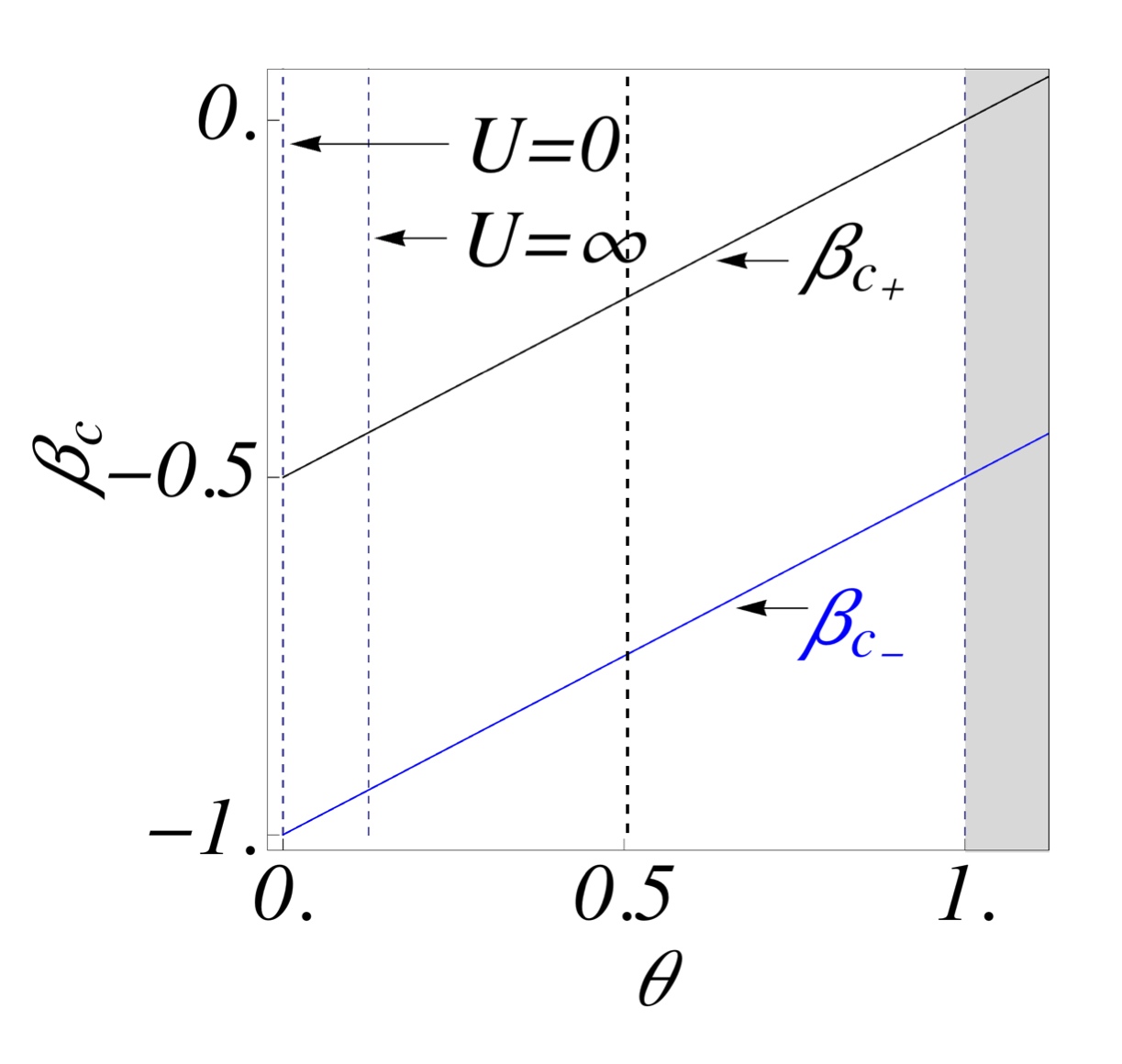
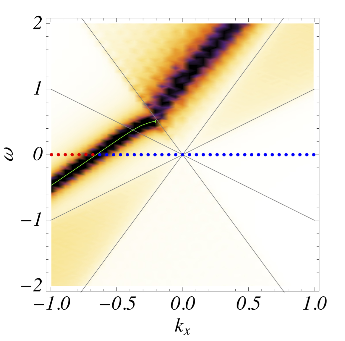
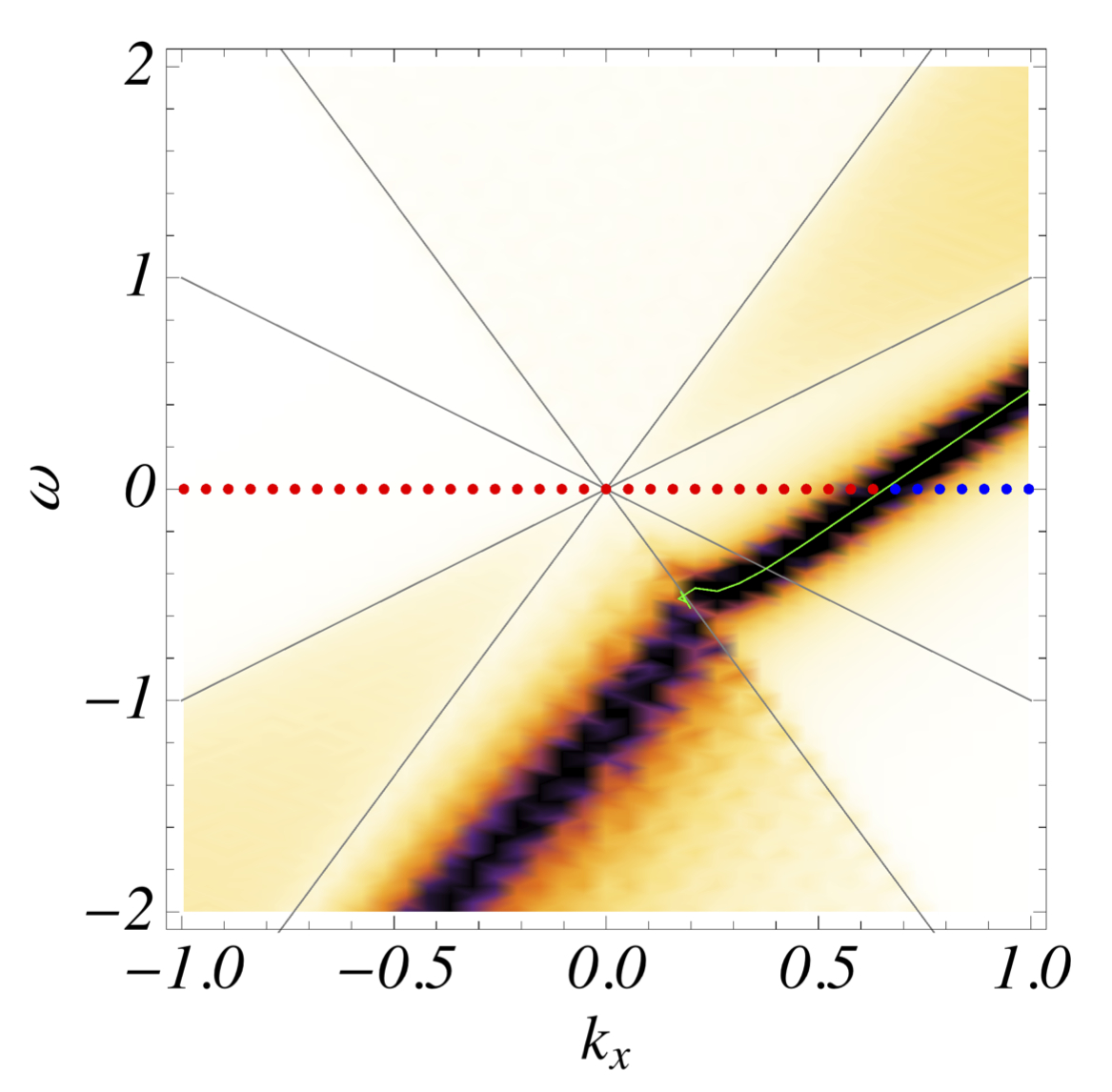
Figure 2: Left Panel: Values of the charge exponents $\beta_{c}^{+}$and $\beta_{c}^{-}$ as a function of the LL parameter $\theta$. Central and Right Panels: Spectral function obtained using the RPA expression (1) for $t^{\prime}=0.2$ and $t^{\prime}=-0.2$ respectively and for $\theta=1/8$, $v_{s}=1$ and $v_{c}=2.718$. The Gray lines signal the boundaries of spin and charge continuum of the 1D spectral function: $\omega=\pm u_{s}k$ and $\omega=\pm u_{c}k$. The bound state (Green line) is obtained solving Eq. (3) . Red and Blue dots displayed at $\omega=0$ correspond to values of $k_{x}$ for which $\text{sign}\text{Re}\left[G\left(\omega=0,k_{x}\right)\right]$ is respectively positive or negative.

In this work we use two approaches to compute the one dimensional spectral function. The first is only valid for low energies and is equivalent to the use of the asymptotic Green’s function given by bosonization. It was used to verify the predictions referred in the last section and to understand the low energy limit of the second approach valid for arbitrary energies. Due to its generality it permits to vary independently the interaction strength (changing $\theta$) as well as the spin and charge velocities. The second approach relies on the exact solution of the large $U$ limit of the Hubbard model. This limit permits considerable simplifications and in particular a closed form for the 1D spectral function. A detailed description of both methods in given in the following sections.

The lowest lying excitations contributing to the spectral function of the 1D Hubbard model correspond to the creation of a holon and a spinon (charge and spin excitations). These two quasiparticles propagate with different velocities and in terms of the original electrons are very complex. Even though they have a fractionalized existence inside the 1D many-body system, when an electron is, for instance, removed from the chain (photoemission) they recombine. If the chains are weakly coupled one expects that the excitations travel along the transverse direction as "electrons". The holon and the spinon are expected to propagate coherently from one chain to the next. This idea was proposed in Ref. Kohno_2007 in the context of an antiferromagnet in a triangular lattice. In the 1D Heisenberg antiferromagnet the low lying excitations are two spinons. In the weak coupling regime they are assumed to propagate coherently from chain to chain (like a $\Delta S=1$ excitation – a magnon). It is therefore interesting to generalize the procedure developed in Ref. Kohno_2007 , for the spin structure factor of the antiferromagnetic Heisenberg model, to the present case of the spectral function of the Hubbard model. This is carried out in Appendix A. There are however difficulties associated with instabilities of the system resulting from the approximation used. The expression obtained for the spectral function is formally very similar to the one obtained within RPA (Appendix C) as noted in ref. Kohno_2007 for the antiferromagnet. A basic difference is that in the RPA the spectral function is defined as a complete function (for positive and negative energies) while in the restricted Hilbert space considered in Appendix A, the positive and negative energies are associated with two functions defined separately. Due to the appearance of bound states one is led to a situation where the excited states have negative energies, which implies an instability of the groundstate. Therefore we will use in the following the RPA expression (1) to obtain the 2D Green’s function. In this context the bound states are interpreted as coherent modes resulting from spectral weight transfer among different energies, as discussed next.

To fix the notation we define the spectral function as

$$Sp\left(\omega,\mathbf{k}\right)=-\frac{1}{\pi}\text{Im}G\left(\omega,\mathbf{k}\right).$$ (7)

In the literature it is usual to write this quantity as a sum $Sp\left(\omega,\mathbf{k}\right)=A(\omega,\mathbf{k})+B(\omega,\mathbf{k})$ where

$$A(\omega,\mathbf{k})=\sum_{f,\sigma}\left|\left\langle f,N+1\right|c_{k,\sigma}^{\dagger}\left|0,N\right\rangle\right|^{2}\delta(\omega-E_{f}^{N+1}+E_{0}^{N})$$ (8)

is the measured amplitude of angular resolved inverse photoemission experiments, here given in the Lehmann representation, and

$$B(\omega,\mathbf{k})=\sum_{f,\sigma}\left|\left\langle f,N-1\right|c_{k,\sigma}\left|0,N\right\rangle\right|^{2}\delta(\omega-E_{0}^{N}-E_{f}^{N-1})$$ (9)

the measured angular resolved photoemission amplitude. $N$ is the number of electrons, $0$ and$f$ denote the ground and final states respectively, the chemical potential is taken such that the ground state corresponds to zero energy so $A(\omega<0,\mathbf{k})=0$ and $B(\omega>0,\mathbf{k})=0$.

III Spectral function at low energies: Luttinger-Liquid-like regime

In this section we concentrate on the low energy region that is characterized by linearized dispersions and power-law behavior, and study how the 2D spectral properties for low energies emerge as a function of $t^{\prime}$ and $\theta$ within the RPA (1). We recover some results by other authors, reviewed in the last section, and find some new features characterizing the different regimes.

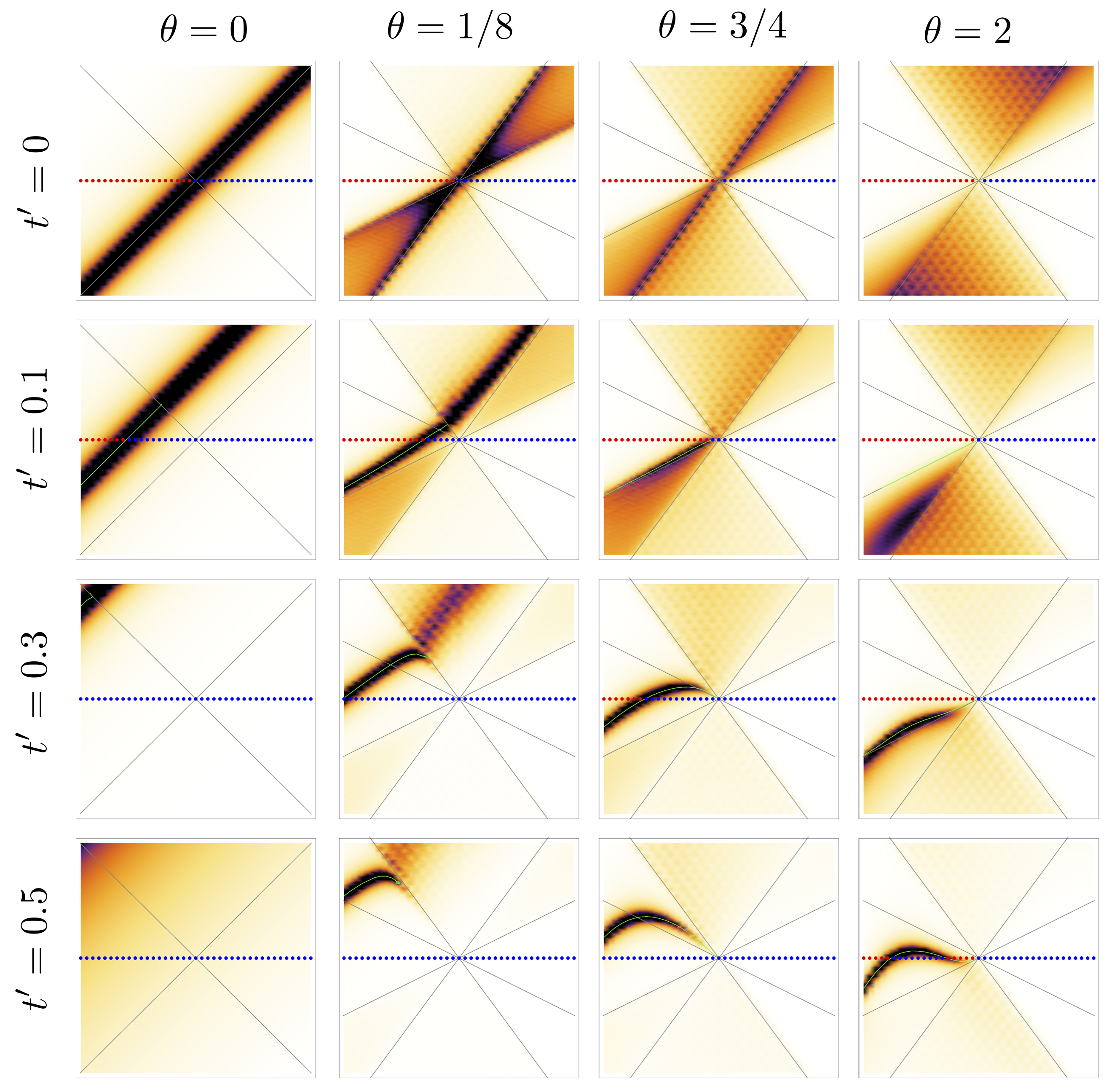
Figure 3: Spectral function obtained by RPA formula (1) for different values of the LL parameter $\theta$ and inter-chain coupling $t^{\prime}$. Axes and labels are the same as for Figs. 2 - Central and Right Panels. For $\theta=0$ we set $v_{c}=v_{s}$ in order to obtain the exact free particle result; for all other values of $\theta$ $v_{s}=1$ and $v_{c}=2.718$. The Gray lines signal the boundaries of spin and charge continuum. Red and Blue dots displayed at $\omega=0$ correspond to values of $k_{x}$ for which $\text{sign}\text{Re}\left[G\left(\omega=0,k_{x}\right)\right]$ is respectively positive or negative. For the cases where $Z\neq 0$ this criterion corresponds to $k_{x}$ being inside or outside the Fermi surface. The Green line corresponds to the bound states obtained solving Eq. (3).

For low energies, and near the Fermi momentum, the spectral function of one dimensional gapless electronic systems can be written as a convolution of the spin and charge parts

$$Sp\left(\omega,k\right) \propto \sum_{i,j;i^{\prime},j^{\prime}\in\mathbb{N}}a_{i,j}^{c}a_{i^{\prime},j^{\prime}}^{s}\left[\delta\left(\omega-\Omega_{i,j}^{c}-\Omega_{i^{\prime},j^{\prime}}^{s}\right)\delta_{k,K_{i,j}+K_{i^{\prime},j^{\prime}}}+\delta\left(\omega+\Omega_{i,j}^{c}+\Omega_{i^{\prime},j^{\prime}}^{s}\right)\delta_{k,-K_{i,j}-K_{i^{\prime},j^{\prime}}}\right]$$ (10)

where $K_{i,j}=2\pi(i-j)/L$ are the momenta of the excitations, $\Omega_{i,j}^{\alpha}=2\pi v_{\alpha}(i+j)/L$ are the corresponding energies (with $\alpha=c,s$ and $v_{s}$ and $v_{c}$ are the spin and charge velocities) and their weights are explicitly given by

$$a_{i,j}^{\alpha} = \frac{\Gamma\left(i+\beta_{\alpha}^{+}+1\right)}{i!\,\Gamma\left(\beta_{\alpha}^{+}+1\right)}\frac{\Gamma\left(j+\beta_{\alpha}^{-}+1\right)}{j!\,\Gamma\left(\beta_{\alpha}^{-}+1\right)}\;.$$ (11)

The exponents $\beta_{c}^{+},\beta_{c}^{-}$ and $\beta_{s}^{+},\beta_{s}^{-}$ characterize the divergence of the spectral function at the edges of the (right, $+$ and left, $-$) charge and spin continua at either the right or left Fermi points. For a Luttinger liquid with SU(2) spin rotation symmetry both $\left\{\beta_{s}^{+},\beta_{s}^{-}\right\}=\left\{-\frac{1}{2},-1\right\}$ are fixed. The charge exponents are given by

$$\left\{\beta_{c}^{+},\beta_{c}^{-}\right\} = \left\{\frac{\theta}{2}-\frac{1}{2},\frac{\theta}{2}-1\right\},$$ (12)

where $\theta$ is related with the Luttinger parameter $K_{c}$ by Eq. (5) (see also Fig.2). As we already mentioned, $\theta=0$ for the noninteracting fermions, and $\theta\rightarrow 1/8$ for $U\rightarrow+\infty$ Hubbard model.

The particular form of the spectral function given by Eq. (10) was obtained in Ref. Penc_1995 in the context of the large $U$ approximation of the Hubbard model. However, the described low energy structure is much more general and can be traced back to the conformal invariance of the (1+1)D model Cardy_1986 . In the thermodynamic limit one obtains the well known asymptotic form, say for the right moving electrons, of the real time Green’s function

$$G_{r}\left(x,t>0\right) \simeq \frac{e^{ik_{F}x}}{(x-v_{c}t)^{1+\beta_{c}^{+}}(x+v_{c}t)^{1+\beta_{c}^{-}}}\times$$

$$\frac{1}{(x-v_{s}t)^{1+\beta_{s}^{+}}(x+v_{s}t)^{1+\beta_{s}^{-}}}$$

that can be directly obtained by bosonization techniques.

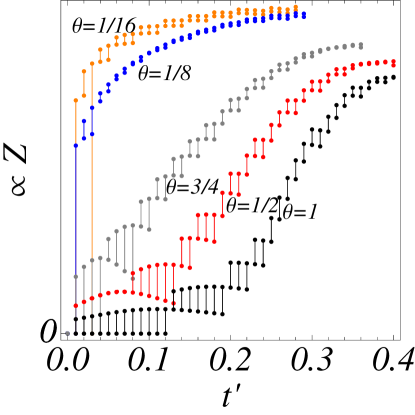
Figure 4: Quasiparticle residue as a function of $t^{\prime}$ for different values of $\theta$: $\theta=1/16$ (Orange), $\theta=1/8$ (Blue), $\theta=1/2$ (Gray) and $\theta=1$ (Black). For each value of $t^{\prime}$, $k_{x}^{+}$ and $k_{x}^{-}$ were determined on each side of the FS. For these values the bound state equation was solved in order to find $\omega_{+/-}\simeq 0$, $Z_{+/-}$ was computed using Eq. (4).

With the 1D Green’s function computed with (10) we used Eq. (1) to obtain the 2D spectral function $Sp\left(\omega,\mathbf{k}\right)=-\frac{1}{\pi}\text{Im}G\left(\omega,\mathbf{k}\right)$ for a fixed value of $t^{\prime}(\mathbf{k})=t^{\prime}$. In Figure 2 - (Central and Right panels) we show the typical results obtained here. The bound states were found solving Eq. (3) outside the spin and charge continua. The FS was determined for the values of $k$ for which $\text{Re}G\left(\omega,\mathbf{k}\right)$ changes sign. Figure 3 displays the main results of this section. The spectral function is shown for different values of the LL parameter $\theta$ and inter-chain coupling $t^{\prime}$. For $\theta=0$ we set $v_{c}=v_{s}$ in order to obtain the exact free particle result; for all other values of $\theta$, fixed values of the spin and charge velocities were used for the physical case $v_{s}<v_{c}$. Fig. 4 shows the values of the QP residue as a function of $t^{\prime}$ for different values of $\theta$. The error bars are due to the discreteness of the $k$ values: for each value of $t^{\prime}$, $k_{x}^{+}$ and $k_{x}^{-}$ were determined on each side of the FS. For these values the bound state equation was solved in order to find $\omega_{+/-}\simeq 0$; $Z_{+/-}$ was then computed using Eq. (4).

As a general feature, we note the change from incoherent regions, arising from the spin-charge separation in the 1D case ($t^{\prime}=0$), to the sharply defined coherent excitations as $t^{\prime}$ increases. For the 1D case the spectral function is strictly zero outside the 1D continuum, delimited by the spin and charge velocities (see 3 upper-left panel). The interchain coupling $t^{\prime}$ favors the appearance of sharp coherent features not only outside the 1D continuum, where they correspond to poles of the 2D Green’s function, but also within the 1D continuum where the spectral weight also tends to concentrate. For $\theta<1$ and small positive $t^{\prime}$($\simeq 0.1$) there is a considerable transfer of spectral weight to the spin (charge) branches for $\omega<0$ ($\omega>0$) . For negative $t^{\prime}$ the spin and charge roles are interchanged (see Fig. 2 - Central and Right Panels). The critical value of $\theta=1$, predicted by several authors Wen_1990 ; Boies_1995 ; Tsvelik_1996 ; Gogolin_1998 , is found such that for $\theta<1$ a bound state appears for $t^{\prime}\neq 0$ crossing $\omega=0$ at $k_{F}(t^{\prime})\neq k_{F}(t^{\prime}=0)$ changing the position of the Fermi surface and resulting in a non-vanishing QP weight $Z$. For $\theta>1$ Fig. 3 shows that for small values of $t^{\prime}$ the bound state still appears. However, since it does not cross $\omega=0$, it is unable to drive the system to a FL like behavior. After some critical $t^{\prime}$ is reached the bound state crosses twice the $\omega=0$ line creating a hole pocket. Note, however, that in this regime the RPA is probably out of its domain of validity and this last feature is probably an artifact. In figure Fig. 3 we show the evolution of the quasiparticle residue as a function of theta. For the region $\theta<1/2$ a damped mode is observed when the coherent mode enters the charge continuum. For $\theta>1/2$ this feature disappears and the coherent mode is deflected to $\omega=0$ and loses all its spectral weight before entering in the continuum. This feature clearly differentiates both regimes. The QP residue as a function of $t^{\prime}$ is shown in Fig. 4. The large error bars obtained due to the discreteness of the values of $k$ prevent a clear fit.

IV Spectral function at finite energies

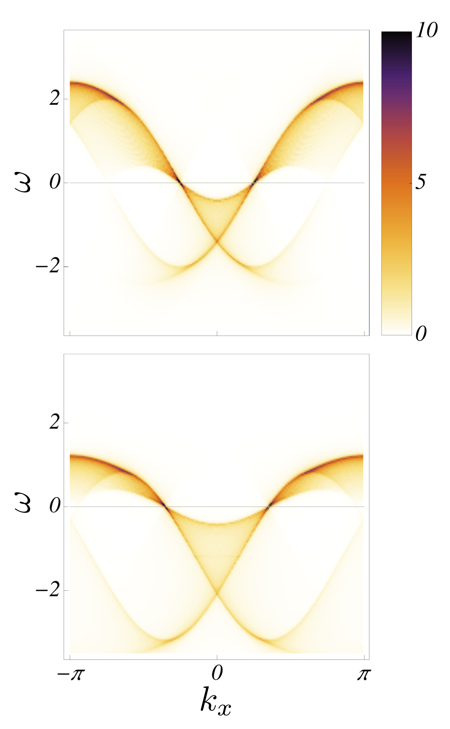
Figure 5: Spectral function for the one dimensional Hubbard Model within the large $U$ approximation. Upper Panel: quarter-filling $n=0.5$, computed for $U/t=7.5$. Lower Panel: $n=0.7$, computed for $U/t=11.5$

In this section we use the spectral function obtained for large $U$ Penc_1997 , together with the RPA expression (1), to compute the finite energy spectral function, for weakly coupled Hubbard chains. The results presented here generalize to finite energies the ones obtained in the previous section for systems that can be well described by an Hubbard like Hamiltonian, with relatively large onsite repulsion ($U/t\gtrsim 6$).

It has been shown that in the $U\to\infty$ limit the eigenstates of the Hubbard chain can be written as a product of a spinless free fermion and a squeezed spin wave functions Woynarovich82 ; Ogata_1990 . In subsequent works Penc_1995 ; Penc_1997 this factorized form was used to write the spectral function as a convolution over the spin and the fermionic parts (see Appendix B). The nontrivial fermionic matrix elements are computed between wave functions of free fermionic states on a ring, with different twisted boundary conditions imposed by the spin configurations. This simplification permitted to obtain the spectral function in the infinite $U$ limit. Note however that if $U\to\infty$ the spin spectrum collapses and the spin sector is completely degenerate.

Once the $t/U$ is finite, the problem can be treated perturbatively, and to get the first order corrections of the energy it is sufficient to look at the expectation value of the perturbing Hamiltonian ($\propto t/U$) with the unperturbed, spin-charge factorized wave functions. When calculating the spectral functions, additional corrections appear in the matrix elements that come from applying the unitary transformation to the electron creation and anihilation operators harris ; oles . For our purposes the most important effect of the finite $t/U$ is to introduce a finite spinon velocity, and that is already captured by the first order corrections to the energy. The spinon velocity at the Fermi momenta is given by

$$v_{s} = \frac{2\pi t^{2}}{U}\left(1-\frac{\sin 2\pi n}{2\pi n}\right)+O\left(\frac{1}{U^{2}}\right),$$ (13)

where $n$ is the band-filling, and the exponents are calculated at the Fermi level.

The results of Penc_1997 and its extension to finite $U$ were proven to be quite accurate for $U/t\gtrsim 6$ (see Carmelo_2006-1 ). Using this method the 1D spectral function was obtained considering systems with size $L$, ranging typically from 120 to 300 sites; quantitative differences as a function of $L$ were observed to be small within this range. Moreover, in order to reduce the computational time, the results presented here used only contributions from one and two particle-hole excitations that were shown to carry the vast majority of the spectral weight ($>99\%$) Penc_1997 ; the inclusion of higher order processes was observed to give neglectable contributions. The values of $U$ were obtained fitting the spin velocity $v_{s}$ with the expression (13), after having computed the 1D spectral function with an effective exchange constant $J_{\text{eff}}$ of the order of $\simeq 0.2$. Using the RPA expression (1), the 2D spectral function was computed for different values of the band filling and transverse momentum. The exact position of the bound state dispersion was obtained as well as the new FS and the dependence of the QP weight. The results are presented in the next sections.

IV.1 Finite large U

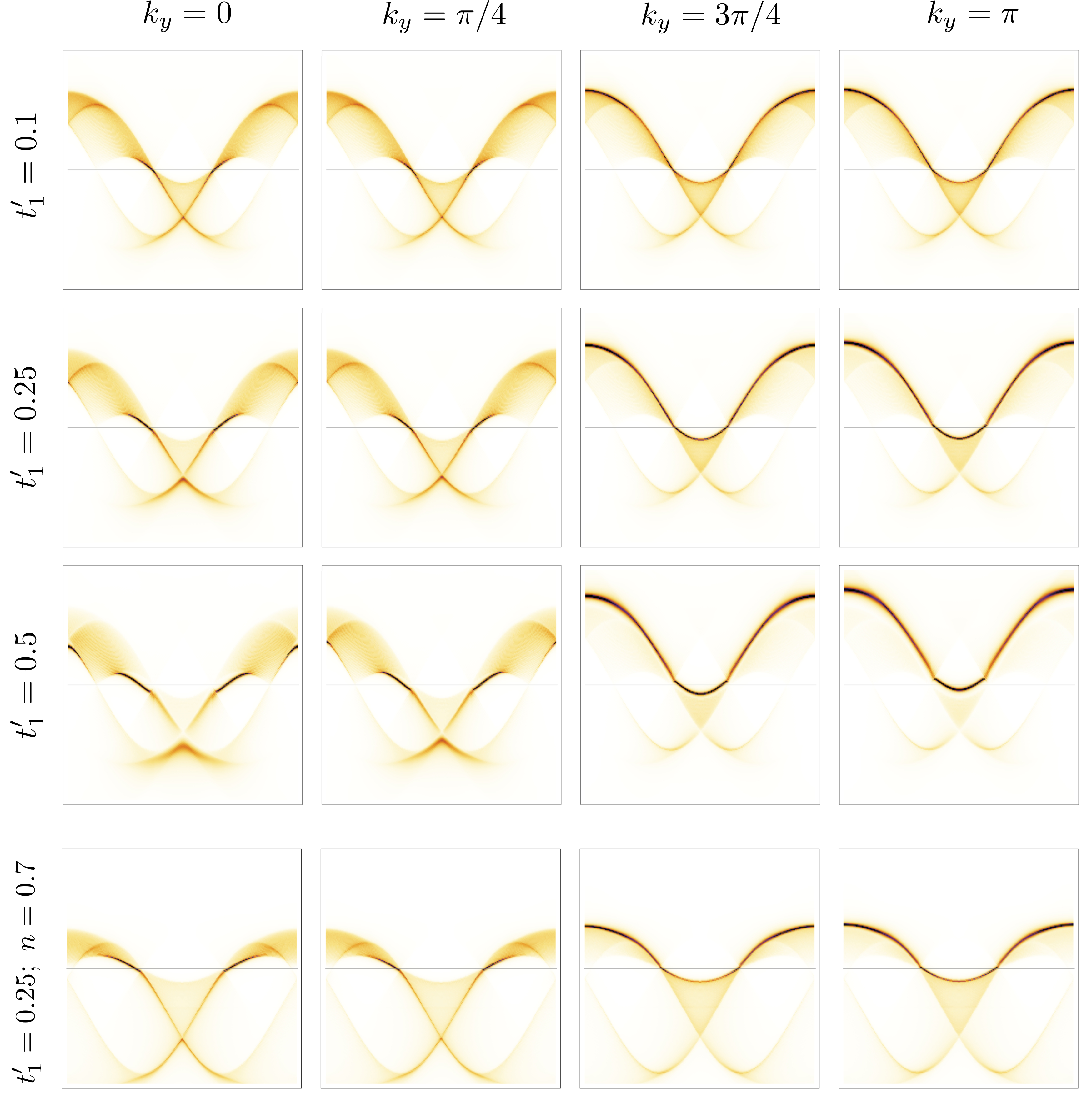
Figure 6: Top 3 rows: Spectral function of the Hubbard model at quarter-filling ($n=0.5$) and $U=7.5$ in an anisotropic square-lattice obtained by weakly coupling Hubbard chains within the RPA (1) for different values of the inter-chain hopping $t^{\prime}_{1}$ and transverse momentum $k_{y}$. The axes labels and the scale are the same as for Figs. 5 . As $t^{\prime}_{1}$ increases the bound states, corresponding to a coherent excitation, start on the boundaries of the continuous region changing the shape of the FS. Lower row: Spectral function of the Hubbard model for $n=0.7$ and $t^{\prime}_{1}=0.25$ and $U/t=11.5$.

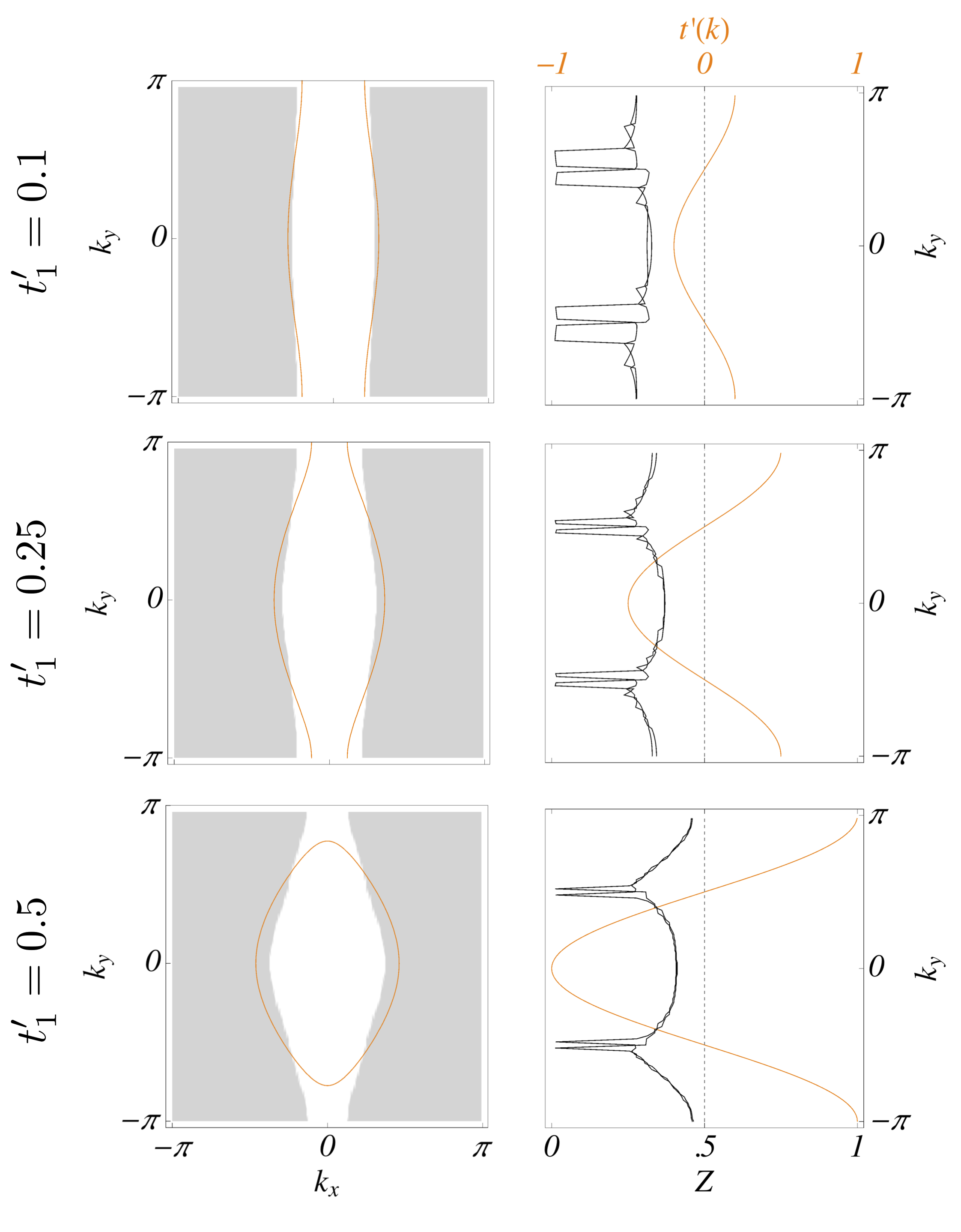
Figure 7: Left Panel: The Gray and White regions correspond, respectively, to $\text{sign}\text{Re}\left[G\left(\omega=0,k_{x}\right)\right]<0$ and $\text{sign}\text{Re}\left[G\left(\omega=0,k_{x}\right)\right]>0$ , i.e. to the exterior and interior of the FS obtained within the RPA. The FS of non-interacting fermions is given by the Orange curves. Right Panel: Quasiparticle residue along the FS as function of $k_{y}$. For each value of $k_{y}$, $k_{x}^{+}$ and $k_{x}^{-}$ were determined on each side of the FS. For these values, the bound-state equation was solved in order to find $\omega_{+/-}\simeq 0$; $Z_{+/-}$ (Black lines) was computed using Eq. (4). The RPA $t^{\prime}\left(\mathbf{k}\right)$ along the FS is plotted as a function of $k_{y}$ (Orange curve). As implied by the RPA expression, when the self energy vanishes the coherent excitations disappear ($Z=0$). Upper, Central and Lower panels correspond respectively to $t^{\prime}_{1}=0.1;\,0.2;\,0.5$ and to $n=0.5$.

Fig. 5 shows the Hubbard chain ($t^{\prime}=0$) spectral function for quarter-filling $(n=0.5)$ and a large value of $U/t=7.5$ and for $n=0.7;$ $U/t=11.5$. Close to zero energy (chemical potential) there is a large spectral weight along both the spinon and holon branch lines. Note that the spectral weight along the spinon branch dies out as we move away from the Fermi level towards positive energies, while the spectral weight along the holon branch line remains high. The branch lines for arbitrary values of the Hubbard coupling, $U$, are obtained moving one excitation (spinon or holon) along its band while keeping the other one fixed at the Fermi level. In the vicinity of the branch line the spectral weight has a power law behavior with exponents that may be negative (yielding a large spectral weight) or positive (leading to an edge and small spectral weight). As shown in Fig. 1 of Ref. Carmelo_2004_b the exponent along the spinon branch line for positive energies changes sign from negative to positive and, therefore, there is a loss of spectral weight, while the exponent along the holon line is always negative.

The 1D results of Fig. 5 are to be compared with those of Fig. 6 where the spectral function is computed for an anisotropic square lattice $(t^{\prime}_{2}=t^{\prime}_{3}=0)$, for different values of the interchain coupling and transverse momentum and for band-fillings $n=0.5,0.7$. Note that since, in this approximation, $t^{\prime}(\mathbf{k})=0$ for $k_{y}=\pi/2$, the SF for this value of the transverse momentum is given by the 1D case of Fig. 5. The low energy behavior near the 1D Fermi momentum agrees with the results of the previous section. In the left panels the effective hopping $t^{\prime}(k)>0$ and in the right panels the effective hopping is $t^{\prime}(k)<0$. As shown in the previous section this implies that for $k_{y}<\pi/2$ the FS increases in size and for $k_{y}>\pi/2$ the FS shrinks. In the 1D case there is a high spectral weight along both the spinon and holon branches at the Fermi surface. Introducing the transverse hopping we find as for the coupled LL that there is an increased spectral weight in one of the two branches depending on the sign of $t^{\prime}(\mathbf{k})$: for $t^{\prime}(k)>0$ at positive energies the weight is concentrated in the spinon branch and at negative energies in the holon branch while the opposite occurs for $t^{\prime}(k)<0$.

Bound states arise near the spinon branch and their weight increases with $t^{\prime}$. For the low energy region the spectral weight outside the 1D continuum is strictly zero due to phase space constraints. In this case the sharp coherent features are poles of the 2D Green’s function. Besides the bound states near $\omega=0$, anti-bound states are formed at high energies. However for the high energy part of the 1D spectrum there is generically no region with strictly zero spectral weight since small contributions will come from higher order particle-hole processes not considered in our method. This means that in practice, contrarily to the boundstates, anti-boundstates will have a small width corresponding to a long, but finite, lifetime of this QP-like excitations. As the transverse hopping increases, all the coherent features become sharper inside and outside the 1D continuum. However, there is still a significant distribution of spectral weight through a continuum, a 1D characteristic. Note that a bound state emerges from the edge of the Brillouin zone that extends to lower energies, as the transverse hopping grows.

In Figure 7 we show the 2D Fermi surface and the quasiparticle residues for different transverse hoppings. The left panels of Fig. 7 show the evolution of the FS as the interchain hopping is increased. Comparison with the non-interacting case (Orange line) shows that interactions will tend to prevent warping of the FS. The Right Panels display the value of $Z$ (black lines) and $t^{\prime}(\mathbf{k})$ (orange lines) along the FS. The QP weight clearly increases with $t^{\prime}_{1}$. Along the FS the inhomogeneities of $Z$ are quite smooth except for the vicinity of $k_{y}=\pi/2$ where it vanishes. As discussed in sec. II.1, since $t^{\prime}(\mathbf{k})=0$ at this point the RPA expression is known to fail. Higher order corrections will give a finite $Z$ value leading to a non-zero QP weight along the FS and thus to FL-like behavior. Note also that even for $t^{\prime}(\mathbf{k})\neq 0$ the RPA underestimates the value of $Z$, so higher order corrections will be expected to slightly increase its value.

IV.2 Infinite U

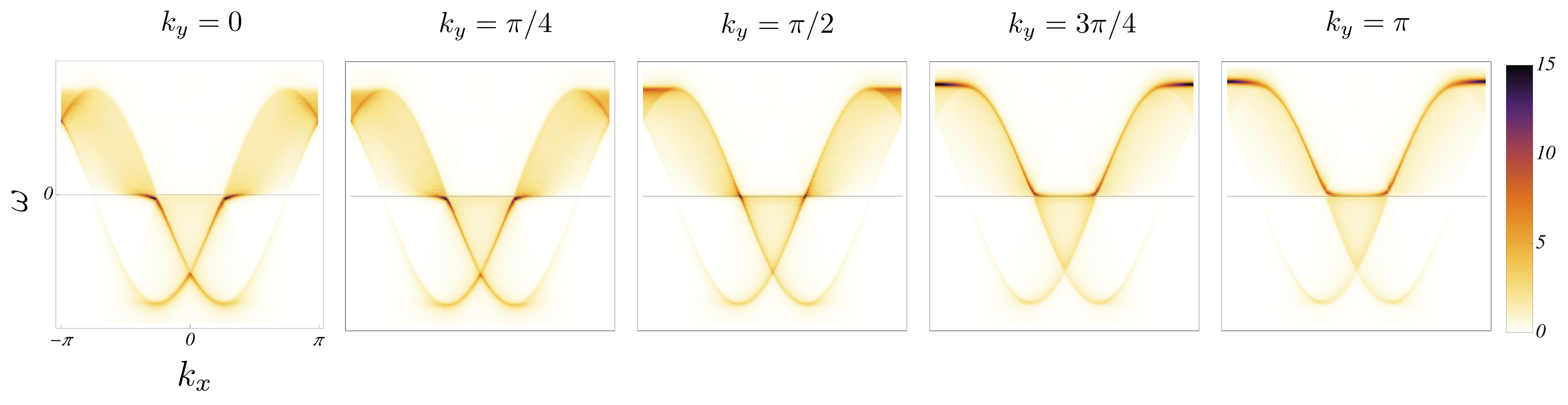
Figure 8: Spectral function of the Hubbard model for $n=0.5$ and $t^{\prime}_{1}=0.25$ for the $U=\infty$ where $u_{s}=0$.

At infinite $U$ the spinons are dispersionless ($J_{\text{eff}}=0$) and the spin velocity vanishes $v_{s}=0$. As a consequence, the lower edges of the continuum, defined by the spinon dispersion relation, become flat and the continuum in these regions extends to zero energy. This is shown in Fig. (8). The central panel for $k_{y}=\pi/2$ displays, as before, the Hubbard chain spectral function. Bound states can still form in the regions where the 1D spectral weight is strictly zero once $t^{\prime}$ is introduced. However, this region is smaller than that for the finite $U$ case. Coherent features also appear at low energies when the bound states enter the continuum. Considering different values of the transverse momentum we see the same trends as for finite $U$. In the left panels there is a "refraction" of the accumulation of spectral weight from a "spinon" branch line at positive energies (note that it is now a flat line since the spinon velocity vanishes in the $U\rightarrow\infty$ limit) and a holon branch at negative energies. In the right panels it is the opposite. However, the antibound states associated with the holon branch also sharpen, even though the distribution of the spectral weight through the continuum is much more visible, as compared to finite $U$. Since the bound states, associated with the spinons do not concentrate much spectral weight, this is to be expected.

V The role of frustration

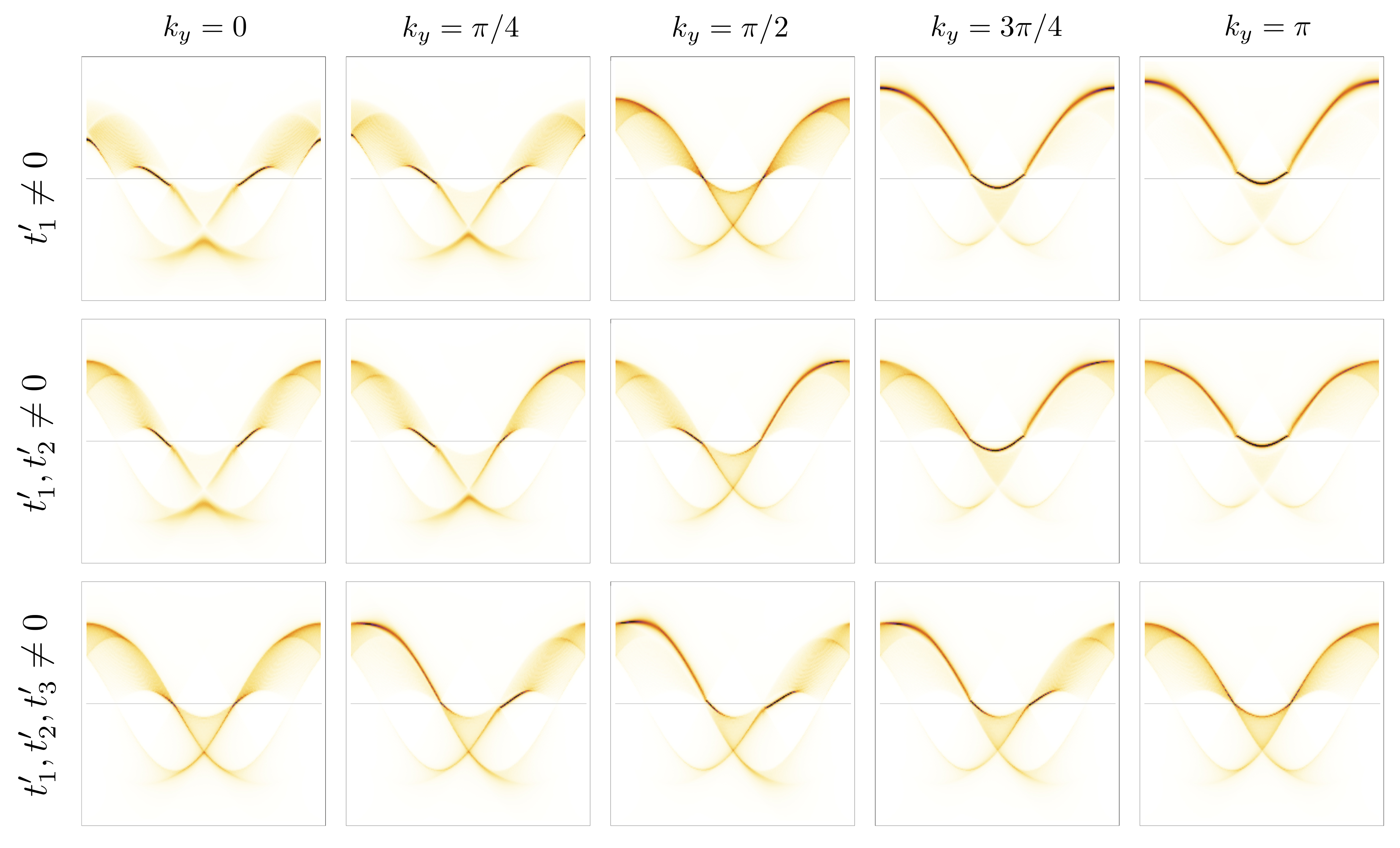
Figure 9: Spectral function of the Hubbard model for several anisotropic lattices: $t^{\prime}_{1}=0.5,t^{\prime}_{2}=t^{\prime}_{3}=0$ (top row); $t^{\prime}_{1}=0.25,t^{\prime}_{2}=0.25,t^{\prime}_{3}=0$ (central row); $t^{\prime}_{1}=0.05,t^{\prime}_{2}=-0.2,t^{\prime}_{3}=0.25$ (bottom row). Note the decrease of coherent modes and the increase of continuum-like features as frustration increases.

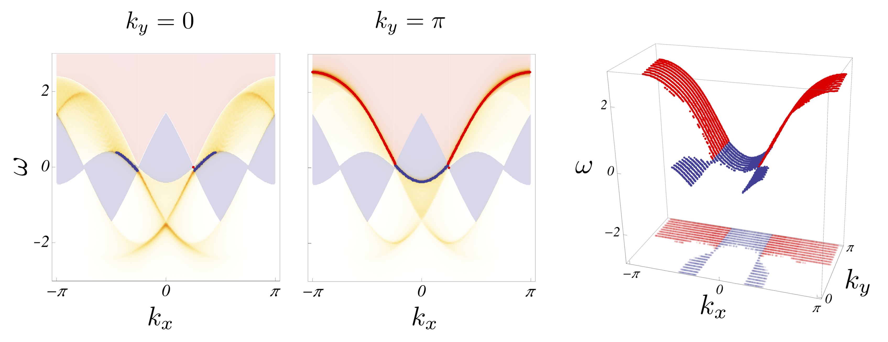
Figure 10: Coherent Modes computed for the anisotropic square lattice with $t^{\prime}_{1}=0.2$ and $U/t=7.5$. Left Panels: Spectral function computed for $k_{y}=0$ and $k_{y}=\pi$. Regions with strictly zero spectral weight are shaded in blue, the boundstate (Blue line) corresponds to a pole of the 2D Green’s function. The high energy regions, shaded in Red, have low but non-vanishing spectral weight, therefore the anti-bound states (Red line) arising in this region have a small but finite width. Right Panel: Dispersion relation of bound and anti-bound states.

It is interesting to see if frustration, in the sence of addition of diagonal terms to the rung ladder-like hoppings, has a similar effect of fractionalization in metallic systems as it does in frustrated magnetic systems. In this section we investigate the role of frustration in the finite energy behavior of the system comparing a non-frustrated lattice (square) with two frustrated lattices, triangular and fully frustrated.

Fig. 9 shows the spectral function computed for an anisotropic square $\left(t^{\prime}_{1}=0.5,t^{\prime}_{2}=t^{\prime}_{3}=0\right)$, triangular $\left(t^{\prime}_{1}=0.25,t^{\prime}_{2}=0.25,t^{\prime}_{3}=0\right)$ and fully frustrated $\left(t^{\prime}_{1}=0.05,t^{\prime}_{2}=-0.2,t^{\prime}_{3}=0.25\right)$ lattices. As the number of frustrated links increases, one observes that the coherent modes are suppressed, as can clearly be seen in Fig. 9 where the incoherent continuum, typical from the 1D case, carries much more spectral weight when compared with the anisotropic square lattice. The reason for the decrease of the coherent features with the degree of frustration, is easy to understand at RPA level. The number of bound and anti-bound states due to $t^{\prime}$, the spectral weight and the distance of the boundstate from the 1D continuum all grow with the magnitude of $t^{\prime}(\mathbf{k})$. Compared to the square lattice, the values of $t^{\prime}(\mathbf{k})$ for frustrated systems vary much more within the Brillouin zone, i.e. even if the maximal value of $\left|t^{\prime}(\mathbf{k})\right|$ is the same for both lattices, stronger oscillations are expected for the frustrated case leading to a smaller mean value $\int d\mathbf{k}\left|t^{\prime}(\mathbf{k})\right|$, which unfavors the appearance of bound-states.

In order to give a quantitative measure of the coherent modes we computed the area of the Brillouin zone occupied by the bound and anti-bound states (see Fig. 10 ). Starting from a square lattice with $t^{\prime}_{1}=0.2$ we have increased the total amplitude of the interchain hopping in three different ways. Table 1 shows the evolution of the area of the Brillouin zone covered coherent modes. For a square lattice, with a larger $t_{1}^{\prime}$, one observes a substantial increase of the area occupied by the bound and anti-bound states: When the same increment is introduced along $t_{2}^{\prime}$ there is a small decrease of the area and a substantial decrease is observed if $t_{3}^{\prime}$ is further increased.

At low energies, two dimensional spin systems and electronic systems near half-filling (where they can be well described by $t-J$ like models), are expected to be rather sensitive to frustration and may develop exotic spin-liquid phases with non-FL behavior. Even if we do not study this low energy regimes, the results presented here do point out that the finite energy spectrum is significantly affected by the frustrated nature of the lattice even if the interchain hopping is small compared with the monitored energy scale.

	$t^{\prime}_{1}=0.2$
	$t^{\prime}_{2}=0.0$
	$t^{\prime}_{3}=0.0$
$t^{\prime}_{1}=0.3$	$t^{\prime}_{1}=0.2$	$t^{\prime}_{1}=0.2$
$t^{\prime}_{2}=0.0$	$t^{\prime}_{2}=0.1$	$t^{\prime}_{2}=0.1$
$t^{\prime}_{3}=0.0$	$t^{\prime}_{3}=0.0$	$t^{\prime}_{3}=0.1$
$\mathbf{\left(+11.0\%\right)}$	$\mathbf{\left(-0.07\%\right)}$	$\mathbf{\left(-16.0\%\right)}$

Table 1: Evolution of the area of the Brillouin zone covered by coherent modes for different values of interchain hopping. The percentage values are relative to the area of the square lattice with $t^{\prime}_{1}=0.2,t^{\prime}_{2}=t^{\prime}_{3}=0.0$ .

VI Discussion

The unusual non-Fermi liquid like properties of some two-dimensional strongly correlated systems has lead to the proposal that some signatures of the exotic properties of one-dimensional systems may be observed in their two-dimensional counterparts. The dimensional crossover from one to two dimensions has been considered by several authors and in most cases it has been found that the one-dimensional features are to a large degree lost, particularly at low energies. One characteristic of the one-dimensional systems is the fractionalization of degrees of freedom which has, however, been shown to persist in some frustrated magnetic systems via the deconfinement of spinons, instead of the coherent magnon-like degrees of freedom characteristic of higher dimensional systems. This apparent fractionalization has been confirmed recently as shown, for instance, in Kohno_2007 .

In this work we have considered Hubbard chains coupled in non-frustrated and frustrated ways and have studied the quasiparticle properties via the spectral function. In order to study the crossover from one to two dimensions we considered spatially anisotropic systems where the interchain couplings (hoppings) are small compared to the intrachain hoppings. The spectral function of the one-dimensional Hubbard model is in general hard to solve but, in some limits, it can be obtained exactly/approximatively such as in the infinite/large U limits. This solution was used to obtain, in the RPA, the two-dimensional spectral function. In the low energy regime a small interchain hopping leads to the formation of a Fermi surface, as shown before by other authors. The appearance of bound states leads to a significant concentration of spectral weight, that extends in some cases to finite energies in a way similar to the formation of coherent modes, as expected in a Fermi liquid like system. However a significant weight is also observed spread through a continuum characteristic of fractionalization of degrees of freedom. This is particularly found when there is frustration in the hoppings, as evidenced by the increase in spectral weight out of the bound states as frustration increases.

It would be interesting to compare these results with experimental results for anisotropic conductors. However, to our knowledge, such systems have not been identified. Some systems show anisotropy but they are not weakly coupled, such as the BEDT systems Kandpal . We expect however that with the advent of fermionic cold atoms in optical lattices the predictions of this work may be tested and new classes of exotic two-dimensional systems may be found.

Appendix A Spectral function in restricted Hilbert space

In this section we discuss the extension of a method, introduced in Kohno_2007 to study anisotropic anti-ferromagnets, to the case of electronic systems. This method permits to write down the 2D spectral function as a function of 1D quantities, in the limit of small inter-chain coupling. The main ingredient is to restrict the Hilbert space to the subspace spanned by eigenstates of decoupled chains with few spinon-chargon pairs. In doing so one neglects some processes that are expected to carry low spectral weight. Besides their formal final resemblance, the expression for the 2D spectral function obtained in this way, follows from fundamentally different approximations than the ones leading to the RPA result. However, we will show explicitly that some problems arise when dealing with this approach, that lead to inconsistencies that prevented us from applying this method.

From the exact one dimensional solution of the Hubbard model one finds a multitude of excitations that can be identified as coming from charge and spin degrees of freedom. However, for practical purposes, single spin-charge excitation characterized by their rapidities carry the vast majority ($>95\%$) of the spectral weight (see Carmelo_2006-1 ). From small to moderate inter-chain coupling, if no phase transition occurs, such excitations are expected to preserve their identity furnishing a natural basis for perturbation theory. The physical picture of the perturbed excitations is given by one dimensional fractionalized electron (or hole) that hops coherently between neighboring chains. These two facts: small inter-chain coupling and low spectral weight of the other types of excitations, allow significant simplification of the problem. The former allows an expansion in small inter-chain coupling and the latter justifies the truncation of the Hilbert space to two particle states.

A.1 Two-particle states

Let the ground state of the unperturbed system ($t^{\prime}_{i}=0$) be denoted by $\left|\mathbf{0}\right\rangle=\otimes_{y}\left|0,y\right\rangle$, with $\left|0,y\right\rangle$ the ground state of the Hubbard Hamiltonian for chain $y$. Its energy is $E_{0}L_{x}L_{y}$, with $E_{0}$ the mean energy per site and $L_{x}$ and $L{}_{y}$ the number of sites in the $x$ and $y$ directions, respectively. From the Bethe Ansatz solution, the two particle states are labeled by the charge and spin rapidities $\nu^{(c)},\nu^{(s)}$ , by the value of the $S_{z}$ component of the spin $\sigma$ and by the total charge of the state $b=\pm 1$, compared to the GS. Such states can be alternatively labeled by their total energy and momentum $\left|\varepsilon_{l},k_{x},\sigma\right\rangle=\left|\nu^{(c)},\nu^{(s)},\sigma\right\rangle$ where $\varepsilon_{l}>0$ and $k_{x}$ are defined by

$$H_{1D}\left|\varepsilon_{l},k_{x},\sigma,b\right\rangle =\left(\varepsilon_{l}+E_{0}L_{x}\right)\left|\varepsilon_{l},k_{x},\sigma,b\right\rangle$$ (14)

$$T\left|\varepsilon_{l},k_{x},\sigma,b\right\rangle =e^{ik_{x}}\left|\varepsilon_{l},k_{x},\sigma,b\right\rangle$$ (15)

where $T$ is the operator that translates the system by one lattice site. For sake of clarity a finite system is considered at this stage, the thermodynamic limit being taken only in the final results; therefore, $\varepsilon_{l}$ and $k_{x}$ are taken within a discrete set of values. The two particle states of the 2D system with momentum $\mathbf{k}=\left(k_{x},k_{y}\right)$ are defined as the Fourier transform in the $y$ direction of the states with only one excited chain:

$$\left|\varepsilon_{l},\mathbf{k},\sigma,b\right\rangle=\frac{1}{\sqrt{L_{y}}}\sum_{y}e^{ik_{y}y}\left|\varepsilon_{l},k_{x},\sigma,b;y\right\rangle\otimes_{y^{\prime}\neq y}\left|0,y^{\prime}\right\rangle$$ (16)

By construction these states are orthogonal to each other as well as to the unperturbed GS, $\left|\mathbf{0}\right\rangle$. The projector to the subspace spanned by the two-particle states and the $t^{\prime}=0$ GS is denoted $\mathbb{P}_{0+2}=\left|\mathbf{0}\right\rangle\left\langle\mathbf{0}\right|+\sum_{\mathbf{k},\sigma,l}\left|\varepsilon_{l},\mathbf{k},\sigma\right\rangle\left\langle\varepsilon_{l},\mathbf{k},\sigma\right|$.

A.2 Spectral Function

The 2D spectral function is obtained as the imaginary part of the retarded Green’s function $Sp_{\sigma}(\omega,\mathbf{k})=-\frac{1}{\pi}\lim_{\eta\to 0}\text{Im}G_{\sigma}^{R}(\omega+i\eta,\mathbf{k})$ defined as

$$G_{\sigma}^{R}(\omega+i\eta,\mathbf{q})$$

$$= \int_{0}^{\infty}dt\ e^{i\left(\omega+i\eta\right)t}(-i)\left\langle\tilde{\mathbf{0}}\right|c_{\mathbf{q},\sigma}(t)c_{\mathbf{q},\sigma}^{\dagger}(0)+c_{\mathbf{q},\sigma}^{\dagger}(0)c_{\mathbf{q},\sigma}(t)\left|\tilde{\mathbf{0}}\right\rangle$$

$$= \sum_{n,\mathbf{k},\sigma^{\prime},b}\left[\frac{\left|\left\langle\tilde{\mathbf{0}}\right|c_{\mathbf{q},\sigma}\left|\Psi_{\mathbf{k},\sigma,b}^{(n)}\right\rangle\right|^{2}}{\omega-\delta E_{\mathbf{k},\sigma,b}^{(n)}+i\eta}+\frac{\left|\left\langle\tilde{\mathbf{0}}\right|c_{\mathbf{q},\sigma}^{\dagger}\left|\Psi_{\mathbf{k},\sigma,b}^{(n)}\right\rangle\right|^{2}}{\omega+\delta E_{\mathbf{k},\sigma,b}^{(n)}+i\eta}\right]$$

with $\left|\tilde{\mathbf{0}}\right\rangle$ the exact GS of the coupled chains. The second equality was obtained using a complete set of eigenstates $\left|\Psi_{\mathbf{k},\sigma,b}^{(n)}\right\rangle$ with energy $E_{\mathbf{k},\sigma,b}^{(n)}=\delta E_{\mathbf{k},\sigma,b}^{(n)}+L_{x}L_{y}E_{0}$. Both $\left|\tilde{\mathbf{0}}\right\rangle$ and $\left|\Psi_{\mathbf{k},\sigma,b}^{(n)}\right\rangle$ will be approximated by their projection in the considered subspace and the effective Hamiltonian is given by $H_{\text{eff}}=\mathbb{P}_{0+2}H\mathbb{P}_{0+2}$.

Using first order perturbation theory in the two-particle subspace one finds:

$$\left|\tilde{\mathbf{0}}\right\rangle \simeq\left|\mathbf{0}\right\rangle+\frac{1}{E_{0}-H_{\parallel}}\mathbb{P}_{0+2}H_{\perp}\mathbb{P}_{0+2}\left|\mathbf{0}\right\rangle+...=\left|\mathbf{0}\right\rangle+O\left(t^{\prime 2}\right)$$ (18)

where the last equality follows since $H_{\perp}$ acting on $\left|\mathbf{0}\right\rangle$ creates two electron-like excitations in neighboring chains which are out of the subspace. Therefore no corrections to the decoupled GS arise in first order in $t^{\prime}$ within the considered subspace. Since $H_{\text{eff}}$ does not couple states with different momentum, total spin or charge one can decompose the eigenstates as

$$\left|\Psi_{\mathbf{k},\sigma,b}^{(n)}\right\rangle=\sum_{l}\ \psi_{\mathbf{k},\sigma,b}(\varepsilon_{l})\left|\mathbf{k},\varepsilon_{l},\sigma,b\right\rangle.$$ (19)

where the summation index runs only over the 1D eigen energies. Computing the matrix elements of $H_{\text{eff}}$ one finds the Schrödinger equation for the amplitudes

$$\psi_{\mathbf{k},\sigma,b}(\varepsilon_{l})\left(\varepsilon_{l}-\delta E_{\mathbf{k},\sigma,b}^{(n)}\right)+b\,t^{\prime}(\mathbf{k})\bar{A}_{b,\sigma}\left(\varepsilon_{l},k_{x}\right)\sum_{l^{\prime}}\ A_{b,\sigma}\left(\varepsilon_{l^{\prime}},k_{x}\right)\psi_{\mathbf{k},\sigma,b}(\varepsilon_{l^{\prime}})=0$$ (20)

where

$$A_{b=-1,\sigma}\left(\varepsilon_{l},k_{x}\right) = \left\langle 0\right|c_{k_{x},\sigma}\left|k_{x},\varepsilon_{l},\sigma,b\right\rangle$$ (21)

$$A_{b=1,\sigma}\left(\varepsilon,k_{x}\right) = \left\langle 0\right|c_{k_{x},\sigma}^{\dagger}\left|k_{x},\varepsilon_{l},\sigma,b\right\rangle$$ (22)

are pure one dimensional quantities and $t^{\prime}(\mathbf{k})$ is the Fourier transform of the transverse hopping matrix (2). For completeness the 1D Green’s function in this notation is given by

$$G_{1D,\sigma}^{R}\left(\omega+i\eta,k_{x}\right) = \sum_{b=\pm}\sum_{l}\frac{A_{b,\sigma}\left(\varepsilon_{l},k_{x}\right)\bar{A}_{b,\sigma}\left(\varepsilon_{l},k_{x}\right)}{\omega+b\,\varepsilon_{l}+i\eta}.$$

Defining $B_{\mathbf{k},\sigma,b}^{(n)}=\sum_{l}\ A_{b,\sigma}\left(\varepsilon_{l},k_{x}\right)\psi_{\mathbf{k},\sigma,b}(\varepsilon_{l})$ and using Eqs. (LABEL:eq:GF_1,21,22) the approximate 2D Green’s function can now be written:

$$G_{\sigma}^{R}(\omega,\mathbf{k}) = \sum_{n,b}\frac{B_{\mathbf{k},\sigma,b}^{(n)}\bar{B}_{\mathbf{k},\sigma,b}^{(n)}}{\omega+b\,\delta E_{\mathbf{k},\sigma,b}^{(n)}+i\eta},$$ (23)

which coincides with the 1D case when $t^{\prime}=0$. Moreover, the particular form of Eq. (20) allows the derivation of the following identities:

$$1 = \,t^{\prime}(\mathbf{k})\sum_{l}\frac{A_{b,\sigma}\left(\varepsilon_{l},k_{x}\right)\bar{A}_{b,\sigma}\left(\varepsilon_{l},k_{x}\right)}{b\left(\delta E_{\mathbf{k},\sigma,b}^{(n)}-\varepsilon_{l}\right)},$$ (24)

$$\left[t^{\prime}(\mathbf{k})^{2}\,B_{\mathbf{k},\sigma,b}^{(n)}\bar{B}_{\mathbf{k},\sigma,b}^{(n)}\right]^{-1} = \sum_{l}\frac{A_{b,\sigma}\left(\varepsilon_{l},k_{x}\right)\bar{A}_{b,\sigma}\left(\varepsilon_{l},k_{x}\right)}{\left(\delta E_{\mathbf{k},\sigma,b}^{(n)}-\varepsilon_{l}\right)^{2}},$$ (25)

where the first equality is obtained by simple manipulations of Eq. (20) and the second follows from imposing unit norm to the eigenstates. These equalities enable the definition of the complex valued functions

$$F_{\mathbf{k},\sigma,b}(z) = \sum_{l}\frac{A_{b,\sigma}\left(\varepsilon_{l},k_{x}\right)\bar{A}_{b,\sigma}\left(\varepsilon_{l},k_{x}\right)}{z-b\,\varepsilon_{l}},$$

with the properties

$$F_{\mathbf{k},\sigma,b}(b\,\delta E_{\mathbf{k},\sigma,b}^{(n)}) = \left[t^{\prime}(\mathbf{k})\right]^{-1},$$ (26)

$$F_{\mathbf{k},\sigma,b}^{\prime}(b\,\delta E_{\mathbf{k},\sigma,b}^{(n)}) = -\left[t^{\prime}(\mathbf{k})^{2}\,B_{\mathbf{k},\sigma,b}^{(n)}\bar{B}_{\mathbf{k},\sigma,b}^{(n)}\right]^{-1}.$$ (27)

So that for a test function $\rho(z)$, analytic in the vicinity of the real line, one has

$$\frac{1}{2\pi i}\oint\ dz\ \rho(z)\,\frac{1}{\left[F_{\mathbf{k},\sigma,b}(z)\right]^{-1}-\,t^{\prime}(\mathbf{k})}=$$ (28)

$$= \sum_{n}\rho(b\,\delta E_{\mathbf{k},\sigma,b}^{(n)})\,B_{\mathbf{k},\sigma,b}^{(n)}\bar{B}_{\mathbf{k},\sigma,b}^{(n)}$$ (29)

where the contour is taken in the domain of analyticity of $\rho(z)$ and encircles anti-clockwise all eigen energies $b\,\delta E_{\mathbf{k},\sigma,b}^{(n)}$. In particular, using $\rho(z)=\frac{1}{\omega-z+i\eta}$, the Green’s function (23) can be written as

$$G_{\sigma}^{R}(\omega+i\eta,\mathbf{k})=$$ (30)

$$\frac{1}{2\pi i}\sum_{b}\oint dz\ \frac{1}{\left[F_{\mathbf{k},\sigma,b}(z)\right]^{-1}-\,t^{\prime}(\mathbf{k})}\frac{1}{\omega-z+i\eta}=$$

$$=\sum_{b}\frac{1}{\left[F_{\mathbf{k},\sigma,b}(\omega+i\eta)\right]^{-1}-\,t^{\prime}(\mathbf{k})}$$

where the contour does not including the $\omega+i\eta$ pole.

A remark about this method is in order at this point. Note the RPA expression given by Eq. (1) so the differences between the two approaches can be clearly observed. Contrarily to the RPA it is not possible to define a single analytic function $F$ gathering both positive and negative energy contributions. This derives from the fact that in the present method Eq.(30) cannot be given as a function of the 1D Green’s function. Instead, each branch has to be summed separately in Eq. (30) in order to obtain the same result as in Eq. (23), which is itself a consequence of the fact that both $b=\pm$ sectors are uncoupled by the Schrödinger equation. Care must be taken when the bound states cross $\omega=0$ in (30); this would correspond to negative excitation energies arising in the Schrödinger equation, signaling an instability of the system. Even though it is still possible to give an expression for the Green’s function in this case, it would not be physically justified to use this result. Since this happens somewhere in the Brillouin zone for the Hubbard model it prevented us to use this method to compute the 2D spectral function. For further comparison we give the spectral and the Green’s function computed with both methods as a function of the 1D spectral function:

Restricted Subspace	RPA
$\begin{array}[]{c}\\ G_{\sigma}^{R}(\omega+i\eta,\mathbf{k})=\sum_{b=\pm 1}\frac{1}{\left[F_{\mathbf{k},\sigma,b}(\omega+i\eta)\right]^{-1}-\,t^{\prime}(\mathbf{k})}\\ \\ \text{where}\\ F_{\mathbf{k},\sigma,b}(\omega+i\eta)=\int d\nu\,\frac{Sp_{1D}\left(\nu,k_{x}\right)\theta\left(b\nu\right)}{\omega+i\eta-\nu}\\ \\ \end{array}$	$\begin{array}[]{c}\\ G_{\sigma}^{R}(\omega+i\eta,\mathbf{k})=\frac{1}{\left[G_{1D}(\omega+i\eta,k_{x})\right]^{-1}-\,t^{\prime}(\mathbf{k})}\\ \\ \text{where}\\ G_{1D}(\omega+i\eta,k_{x})=\int d\nu\,\frac{Sp_{1D}\left(\nu,k_{x}\right)}{\omega+i\eta-\nu}\\ \\ \end{array}$
$\begin{array}[]{c}\\ Sp(\varepsilon,\mathbf{k})=\sum_{b=\pm 1}\frac{\chi_{\mathbf{k},\sigma,b}^{{}^{\prime\prime}}(\varepsilon)/\pi}{\left[1-t^{\prime}(\mathbf{k})\chi_{\mathbf{k},\sigma,b}^{{}^{\prime}}(\varepsilon)\right]^{2}+\left[t^{\prime}(\mathbf{k})\chi_{\mathbf{k},\sigma,b}^{{}^{\prime\prime}}(\varepsilon)\right]^{2}}\\ +\sum_{p,b}\frac{1}{F_{\mathbf{k},\sigma,b}^{-1^{\prime}}(z_{p})}\delta\left(\varepsilon-z_{p}\right)\\ \\ \text{where}\\ \chi_{\mathbf{k},\sigma,b}^{{}^{\prime\prime}}(\varepsilon)=\pi Sp_{1D}\left(\varepsilon,k_{x}\right)\theta\left(b\varepsilon\right)\\ \chi_{\mathbf{k},\sigma,b}^{{}^{\prime}}(\varepsilon)=P\int d\nu\,\frac{Sp_{1D}\left(\nu,k_{x}\right)\theta\left(b\varepsilon\right)}{\varepsilon-\nu}\\ \\ \end{array}$	$\begin{array}[]{c}\\ Sp(\varepsilon,\mathbf{k})=\frac{\chi_{\mathbf{k},\sigma}^{\left(\text{RPA}\right)^{\prime\prime}}(\varepsilon)/\pi}{\left[1-t^{\prime}(\mathbf{k})\chi_{\mathbf{k},\sigma}^{\left(\text{RPA}\right)^{\prime}}(\varepsilon)\right]^{2}+\left[t^{\prime}(\mathbf{k})\chi_{\mathbf{k},\sigma}^{\left(\text{RPA}\right)^{\prime\prime}}(\varepsilon)\right]^{2}}\\ +\sum_{p}\frac{1}{G_{1D}^{-1^{\prime}}(z_{p},k_{x})}\delta\left(\varepsilon-z_{p}\right)\\ \\ \text{where}\\ \chi_{\mathbf{k},\sigma}^{\left(\text{RPA}\right)^{\prime\prime}}(\varepsilon)=\pi Sp_{1D}\left(\varepsilon,k_{x}\right)\\ \chi_{\mathbf{k},\sigma}^{\left(\text{RPA}\right)^{\prime}}(\varepsilon)=P\int d\nu\,\frac{Sp_{1D}\left(\nu,k_{x}\right)}{\varepsilon-\nu}\\ \\ \end{array}$

In the above expressions the thermodynamic limit was taken replacing $\sum_{l}$$\rho(\varepsilon_{l},k_{x},\sigma,b)$ by $\int d\nu\ D_{k_{x},\sigma,b}\left(\nu\right)\rho(\nu)$, where $D_{k_{x},\sigma,b}\left(\nu\right)$ is the one dimensional density of states with quantum numbers $k_{x},\sigma,b$, and using the definition $Sp_{1D}\left(\varepsilon,k_{x}\right)=\sum_{b}D_{k_{x},\sigma,b}\left(b\varepsilon\right)A_{b,\sigma}\left(b\varepsilon,k_{x}\right)\bar{A}_{b,\sigma}\left(b\varepsilon,k_{x}\right)$. Note that when this replacement is done, the Green’s function acquires a branch cut in the support of $D_{k_{x},\sigma,b}\left(b\nu\right)$ and coherent contributions from the simple poles for both methods. Corrections to the effective Hamiltonian method can be included as in Ref. in Kohno_2007 by considering a larger subspace spanned by states containing higher ordered processes along a chain and/or where more than one chain is in an excited state. In the generic case the GS will also have corrections (see Eq. (18)) of higher order in $t^{\prime}$.

Appendix B Factorized wave function and spectral function

In the $U\rightarrow+\infty$ limit of the Hubbard model the doubly occupied sites are forbidden, and the electrons with opposite spins cannot jump over each other - the sequence of the spins of the electrons is fixed. As a consequence, the wave functions can be written in a factorized form,

$$|\Psi_{P}^{N}\rangle=|\psi_{L,Q}^{N}(\{I\})\rangle\otimes|\chi_{N}^{N_{\downarrow}}(Q,\tilde{f}_{Q})\rangle$$ (31)

where $|\chi\rangle$ stands for the spin-part of the $N$ electrons that is defined on a fictitious lattice of the $N$ sites, with the wave vector $Q=2\pi K/N$ ($K=0,\dots,N-1$ is an integer) and $\tilde{f}_{Q}$ are some other quantum numbers Woynarovich82 ; Ogata_1990 . The $|\psi\rangle$ describes the $N$ electrons as spinless free fermions with twisted boundary condition imposed by the spins:

$$Lk_{j}=2\pi I_{j}+Q$$ (32)

where the wave vector $Q$ of the spin wave function appears as a phase shift and $I_{j}=0,\dots,L-1$. The total momentum and energy of the state are given by

$$P = \sum_{j}k_{j}=\frac{2\pi}{L}\sum_{j}I_{j}+\frac{N}{L}Q=\frac{2\pi}{L}\left(\sum I_{j}+K\right)$$

$$E = -2t\sum_{j}\cos k_{j}$$

Strictly speaking, for $U=+\infty$ all the spin wave function are degenerate in energy, and the $U\rightarrow+\infty$ limit is taken such that in the ground state the $|\chi\rangle$ coincides with the ground state of the Heisenberg model, with wave vector $Q=\pi$.

The electron addition and removal spectral functions are then given as

$$A(k,\omega) = \sum_{Q}C(Q)A_{Q}(k,\omega)$$ (33)

$$B(k,\omega) = \sum_{Q}D(Q)B_{Q}(k,\omega)$$ (34)

where the $A_{Q}(k,\omega)$ and $B_{Q}(k,\omega)$ are coming from the charge, and $C(Q)$ and $D(Q)$ from the spin part of the wave function and can be evaluated as described in Ref. Penc_1997 . We note the absence of the energy scale in the spin part.

For finite values of $U/t$ the spin part gets finite dispersion. As it has been noted in Penc_1997 (see also Ref. talstra ), in the $\omega$-resolved $C(Q,\omega)$ and $D(Q,\omega)$ the weight is to large extent concentrated on the lower edge of the continuum, following the dispersion of the one-spinon branch (we note that the number of spinons in the final states is odd, since we had added one spinon to the initial spin wave function), so that

$$C(Q,\omega) = C(Q)\delta(\omega-\varepsilon_{s}-\varepsilon_{Q}),$$

$$D(Q,\omega) = D(Q)\delta(\omega-\varepsilon_{s}+\varepsilon_{Q}),$$

where $\varepsilon_{Q}$ is the des Cloizeaux-Pearson dispersiondesCLoizeaux ; spinon

$$\varepsilon_{Q}=\frac{\pi}{2}J_{\text{eff}}|\sin(Q-\pi/2)|\;,$$ (35)

and

$$J_{\text{eff}}=n\left(1-\frac{\sin 2\pi n}{2\pi n}\right)\frac{4t^{2}}{U}$$ (36)

is the effective exchange in the $N$-site Heisenberg model of the spin part. After the convolution with the $A_{Q}(\omega,k)$ and $B_{Q}(\omega,k)$ charge part, the inclusions of the spinon dispersion given above provides a finite spinon dispersion that is seen in Fig. 5: it defines the lower edge of the $A(\omega,k)$ for the $k$ values between the $k_{F}$ and the $3k_{F}$, and the lower edge of the $B(\omega,k)$ for $-k_{F}<k<k_{F}$.

Appendix C RPA and next to leading order corrections

In this section we rederive the RPA results obtained before by many authors and give explicitly the next to leading order corrections. However, since 1D correlation functions of higher order are needed in order compute these corrections they were not included in the computation of the spectral function in the main text.

The partition function of the model with Grassmanian sources is given by

$$Z\left[\zeta^{\dagger},\zeta\right] = \int Dc^{\dagger}Dc\ e^{-\int_{\tau}\left[\sum_{\mathbf{k},\sigma}c_{\mathbf{k},\sigma}^{\dagger}(\tau)\partial_{\tau}c_{\mathbf{k},\sigma}(\tau)+:H(\tau):-\sum_{\mathbf{k},\sigma}\left(\zeta_{\mathbf{k},\sigma}^{\dagger}(\tau)c_{\mathbf{k},\sigma}(\tau)+c_{\mathbf{k},\sigma}^{\dagger}(\tau)\zeta_{\mathbf{k},\sigma}(\tau)\right)\right]}$$ (37)

$$= Z_{\parallel}\left\langle e^{\mathbf{c}^{\dagger}.\mathbf{t}^{\prime}.\mathbf{c}+\boldsymbol{\zeta}^{\dagger}.\mathbf{c}+\mathbf{c}^{\dagger}.\boldsymbol{\zeta}}\right\rangle_{\parallel}$$

where $Z_{\parallel}$ and $\left\langle...\right\rangle_{\parallel}$ are respectively the partition function and the expectation value of an operator in absence of interchain coupling and $H=H_{\parallel}+\sum_{ij}c_{i}^{\dagger}t^{\prime}_{ij}c_{j}$. The compact notation $\mathbf{c}^{\dagger}.\mathbf{t}^{\prime}.\mathbf{c}=\int d\tau\ \sum_{\mathbf{k},\sigma}c_{\mathbf{k},\sigma}^{\dagger}(\tau)t^{\prime}\left(\mathbf{k}\right)c_{\mathbf{k},\sigma}(\tau)$ and $\boldsymbol{\zeta}^{\dagger}.\mathbf{c}=\int d\tau\sum_{\mathbf{k},\sigma}\zeta_{\mathbf{k},\sigma}^{\dagger}(\tau)c_{\mathbf{k},\sigma}(\tau)$ was introduced to improve the readability of the expressions and will be used in the rest of this section. Inserting a Grassmanian Hubbard-Stratonovich (HS) field $\psi$ to decouple the hopping term and performing a subsequent shift in this field in order to let the term within brackets independent from the sources one gets

$$Z\left[\zeta^{\dagger},\zeta\right] =Z_{\parallel}\int D\psi^{\dagger}D\psi\ e^{-N\,F}$$ (38)

with

$$F = -\left(\boldsymbol{\psi}^{\dagger}+\boldsymbol{\zeta}^{\dagger}\right).\mathbf{t}^{\prime-1}.\left(\boldsymbol{\psi}+\boldsymbol{\zeta}\right)-\ln\left\langle e^{\boldsymbol{\psi}^{\dagger}\mathbf{c}+\mathbf{c}^{\dagger}\boldsymbol{\psi}}\right\rangle_{\parallel}.$$

$N=1$ for the physical case, but we will nevertheless perform a saddle point approximation in Eq. (38) which can be seen as an expansion around $N\to\infty$. This method is similar to the one considered in Boies_1995 . When the HS variables are bosons such procedure is equivalent to a given mean field decoupling. The saddle point value is defined by $\delta_{\boldsymbol{\psi}}F=\left(\boldsymbol{\psi}^{\dagger}+\boldsymbol{\zeta}^{\dagger}\right).\mathbf{t}^{\prime-1}+\left\langle\mathbf{c}^{\dagger}\right\rangle_{\parallel\psi}$ with $\left\langle...\right\rangle_{\parallel\psi}=\left\langle e^{\boldsymbol{\psi}^{\dagger}\mathbf{c}+\mathbf{c}^{\dagger}\boldsymbol{\psi}}\right\rangle_{\parallel}^{-1}\left\langle...\,e^{\boldsymbol{\psi}^{\dagger}\mathbf{c}+\mathbf{c}^{\dagger}\boldsymbol{\psi}}\right\rangle_{\parallel}$. Assuming that $t^{\prime}\ll 1$ the saddle point value is $\psi=0$ when computed at $\zeta=0$. To quadratic order one obtains

$$Z\left[\zeta^{\dagger},\zeta\right] = Z_{\parallel}e^{-N\,\left\{F-\frac{1}{N}\frac{1}{2}\text{Tr}\ln\left[-\delta^{2}F\right]\right\}}\times$$ (40)

$$\times\left[1+O\left(\frac{1}{N}\right)\right]$$

where $\delta^{2}F_{i,j}=\delta_{\Psi_{i}}\delta_{\Psi_{j}}F$ with $\Psi=(\psi,\psi^{\dagger})$ is the second derivative matrix

$$\delta^{2}F_{\bar{i},j} = \delta_{\Psi_{i}^{\dagger}}\delta_{\Psi_{j}}F$$

$$= \left(\begin{array}[]{cc}\mathbf{t}^{\prime-1}+\left\langle\mathbf{c}\mathbf{c}^{\dagger}\right\rangle_{\parallel}&-\left\langle\mathbf{c}\mathbf{c}\right\rangle_{\parallel}\\ \left\langle\mathbf{c}^{\dagger}\mathbf{c}^{\dagger}\right\rangle_{\parallel}&-\mathbf{t}^{\prime-1}+\left\langle\mathbf{c}^{\dagger}\mathbf{c}\right\rangle_{\parallel}\end{array}\right)_{i,j}$$

which is diagonal since the anomalous terms vanish. The Green’s function is obtained taking derivatives with respect to the sources

$$G_{\alpha,\alpha^{\prime}} = \frac{1}{N}\left.d_{\zeta_{\alpha}^{\dagger}}d_{\zeta_{\alpha^{\prime}}}\ln Z\left[\zeta^{\dagger},\zeta\right]\right|_{\zeta=0}$$

$$= \left.-\delta_{\zeta_{\alpha}^{\dagger}}\delta_{\zeta_{\alpha^{\prime}}}F+\frac{1}{2N}\text{Tr}\left[\delta^{2}F^{-1}\left(\delta_{\zeta_{\alpha}^{\dagger}}\delta_{\zeta_{\alpha^{\prime}}}\delta^{2}F\right)\right]\right|_{\zeta=0}$$

$$+O\left(\frac{1}{N^{2}}\right)$$

where $d_{\zeta_{\alpha}^{\dagger}}=\delta_{\zeta_{\alpha}^{\dagger}}+\left(\delta_{\zeta_{\alpha}^{\dagger}}\Psi_{i}\right)\delta_{\Psi_{i}}$ stands for the total variation and $\delta$ for explicit one. Using the saddle point condition $\delta_{\Psi_{j}}F=0$ and total variations of this relation one obtains

$$G_{\alpha,\alpha^{\prime}}^{-1} = \tilde{G}_{\alpha\alpha^{\prime}}^{-1}-\frac{1}{N}\tilde{G}_{m^{\prime}n^{\prime}}\tilde{\Gamma}_{\alpha n^{\prime}m^{\prime}\alpha^{\prime}}+O\left(\frac{1}{N^{2}}\right)$$ (42)

where we have defined the bare $\left(t^{\prime}=0\right)$ propagator and the propagator at RPA level respectively as

$$G_{\parallel\alpha l^{\prime}} = -\left[\left\langle\boldsymbol{c}\boldsymbol{c}^{\dagger}\right\rangle_{\parallel}\right]_{\alpha l^{\prime}}$$ (43)

$$\tilde{G}_{\alpha l^{\prime}} = -\left[\left\langle\boldsymbol{c}\boldsymbol{c}^{\dagger}\right\rangle_{\parallel}^{-1}+\mathbf{t}^{\prime}\right]_{\alpha l^{\prime}}^{-1}$$ (44)

as well as the four point function

$$\tilde{\Gamma}_{l^{\prime}n^{\prime}m^{\prime}i^{\prime}} = \mathbf{t}^{\prime}_{mm^{\prime}}\left[G_{\parallel l^{\prime}l}^{-1}G_{\parallel n^{\prime}n}^{-1}G_{\parallel i^{\prime}i}^{-1}\left\langle c_{l}c_{n}c_{m}^{\dagger}c_{i}^{\dagger}\right\rangle_{\parallel C}\right]$$

where $\left\langle...\right\rangle_{\parallel C}$ stands for the connected correlator.

In standard notation with $k=\left(i\omega_{n},\mathbf{k}_{\parallel},\mathbf{k}_{\perp},\sigma\right)$ and $\int_{q}=\frac{1}{\beta}\sum_{\omega_{n}}\sum_{\mathbf{q},\sigma}$, expression (42) translates to

$$G\left(k\right) = \left[\tilde{G}\left(k\right)^{-1}-\frac{1}{N}\int_{q}\tilde{G}\left(q\right)\tilde{\Gamma}_{4}\left(k,q\right)\right]^{-1}$$ (46)

$$+O\left(\frac{1}{N^{2}}\right),$$

where expressions (44) and (LABEL:eq:Ver_RPA_mat) are respectively given by

$$\tilde{G}\left(k\right) = \left[G_{\parallel}\left(k_{\parallel}\right)^{-1}-t^{\prime}\left(\mathbf{k}\right)\right]^{-1},$$ (47)

$$\tilde{\Gamma}_{4}\left(k,q\right) = t^{\prime}\left(\mathbf{q}\right)\Gamma_{1D}\left(k_{\parallel},q_{\parallel}\right),$$ (48)

with $k_{\parallel}=\left(i\omega_{n},\mathbf{k}_{\parallel},\sigma\right)$ and where $G_{\parallel}\left(k_{\parallel}\right)$ is the one-dimensional Green’s function. The one dimensional quantity

$$\Gamma_{1D}\left(k_{\parallel},q_{\parallel}\right) = \frac{\left\langle c_{k_{\parallel}}c_{q_{\parallel}}c_{q_{\parallel}}^{\dagger}c_{k_{\parallel}}^{\dagger}\right\rangle_{\parallel C}}{G_{\parallel}\left(q_{\parallel}\right)G_{\parallel}\left(k_{\parallel}\right)G_{\parallel}\left(k_{\parallel}\right)}$$ (49)

is given as a function of the 1D form factors and propagators. Eqs. (46-49) permit to obtain the 2D propagator as a function of the 1D quantities only. This expression involves higher order correlation functions for the Hubbard chain which are not known at this point.

References

- (1) E.H. Lieb and F.Y. Wu, Phys. Rev. Lett., 20, 1445 (1968).
- (2) F.D.M. Haldane, J. Phys. C 14, 2585 (1981).
- (3) T. Giamarchi, "Quantum Physics in One Dimension", Oxford University Press (2003).
- (4) A. O. Gogolin , A. A. Nersesyan, A. M. Tsvelik, Bosonization and Strong Correlated Systems, Cambridge University Press, Cambridge England, (1998)
- (5) J. Voit, Rep. Prog. Phys. 58, 977 (1995).
- (6) H. Frahm, V. E. Korepin, Phys. Rev. B 42, 10553 (1990); Phys. Rev. B 43, 5653 (1991).
- (7) J.M.P. Carmelo, F. Guinea, P.D. Sacramento, Phys. Rev. B 55, 7565 (1997).
- (8) K. Penc, F. Mila and H. Shiba, Phys. Rev. Lett., 75, 894 (1995).
- (9) K. Penc, K. Hallberg, F. Mila and H. Shiba, Phys. Rev. Lett., 77, 1390 (1996).
- (10) F.H.L. Essler and V.E. Korepin, Phys. Rev. B 59, 1734 (1999).
- (11) M. Sing, U. Schwingenschlögl, R. Claessen, P. Blaha, J.M.P. Carmelo, L.M. Martelo, P.D. Sacramento, M. Dressel, and C.S. Jacobsen, Phys. Rev. B, 68, 125111 (2003).
- (12) J.M.P. Carmelo, J.M. Roman, and K. Penc, Nucl. Phys. B, 683, 387 (2004).
- (13) J. M. P. Carmelo, K. Penc, L. M. Martelo, P. D. Sacramento, J. M. B. Lopes dos Santos, R. Claessen, M. Sing and U. Schwingenschlögl, Europhys. Lett., 67, 233 (2004).
- (14) J.M.P. Carmelo and K. Penc, Eur. Phys. J. B, 51, 477 (2006).
- (15) D. Bozi, J.M.P. Carmelo, K. Penc and P.D. Sacramento, J. Phys.: Condens. Matter, 20, 022205 (2008).
- (16) R.B. Laughlin, Phys. Rev. Lett. 50, 1395 (1983); C. L. Kane and M. P. A. Fisher, Phys. Rev. Lett. 72, 724 (1994);
- (17) L. Saminadayar, D. C. Glattli, Y. Jin, and B. Etienne, Phys. Rev. Lett. 79, 2526 (1997). R. de-Picciotto, M. Reznikov, M. Helbium, V. Umansky, G. Bunin and D. Mahalu, Nature Lett. 389, 162 (1997).
- (18) P. Fulde, K. Penc, and N. Shannon, Ann. Phys. (Leipzig) 11, 892 (2002); C. Hotta and F. Pollmann Phys. Rev. Lett. 100, 186404 (2008).
- (19) S. Sachdev, Phys. Rev. B 45, 12377 (1992).
- (20) R. Coldea, D. A. Tennant, A. M. Tsvelik and Z. Tylazynski, Phys. Rev. Lett. 86, 1335 (2001).
- (21) J. des Cloizeaux and J. J. Pearson, Phys. Rev. 128, 2131 (1962); T. Yamada, Prog. Theor. Phys. Jpn. bf 41, 880 (1969).
- (22) M. Kohno , O.A. Starykh, L. Balents, Nature Physics, 3, 790 (2007).
- (23) I. U. Heilmann et al., Phys. Rev. B 18, 3530 (1978).
- (24) S. E. Nagler et al., Phys. Rev. B 44, 12361 (1991); D. A. Tennant, T. G. Perring, R. A. Cowley and S. E. Nagler, Phys. Rev. Lett. 70, 4003 (1993).
- (25) D. A. Tennant, R. A. Cowley, S. E. Nagler and A. M. Tsvelik, Phys. Rev. B 52, 13368 (1995).
- (26) D. C. Dender et al., Phys. Rev. B 53, 2583 (1996).
- (27) K. Penc, K. Hallberg, F. Mila, and H. Shiba, Phys. Rev. B, 55, 15475 (1997).
- (28) X.G. Wen, Phys. Rev. B, 42, 6623 (1990).
- (29) K. Ueda and T. M. Rice, Phys. Rev. B, 29, 1514 (1984). C. Castellani, C. Di Castro, and W. Metzner, Phys. Rev. Lett., 72, 316 (1994).
- (30) D. Boies, C. Bourbonnais and A.-M.S. Tremblay, Phys. Rev. Lett., 74, 968 (1995).
- (31) E. Arrigoni, Phys. Rev. Lett., 80, 790 (1998).
- (32) E. Arrigoni, Phys. Rev. Lett., 83, 128 (1999).
- (33) E. Arrigoni, Phys. Rev. B, 61, 7909 (2000).
- (34) P. Kopietz, V. Meden and K. Schönhammer, Phys. Rev. Lett., 74, 2997 (1995).
- (35) P. Kopietz, V. Medenr and K. Schönhammer, Phys. Rev. B, 56, 7232 (1997).
- (36) L. Balents, M. P. A. Fisher, Phys. Rev. B 53, 12133 (1996).
- (37) H.-H. Lin, L. Balents, M. P. A. Fisher, Phys. Rev. B 56, 6569 (1997).
- (38) C. Wu, W. V. Liu, E. Fradkin, Phys. Rev. B 68, 115104 (2003).
- (39) J.C. Nickel, R. Duprat, C. Bourbonnais, and N. Dupuis, Phys. Rev. Lett., 95, 247001 (2005).
- (40) J.C. Nickel, R. Duprat, C. Bourbonnais, and N. Dupuis, Phys. Rev. B, 73, 165126 (2006).
- (41) D. G. Clarke, S. P. Strong, and P. W. Anderson , Phys. Rev. Lett. 72, 3218 (1994).
- (42) D. Poilblanc, H. Endres, F. Mila, M. G. Zacher, S. Capponi, W. Hanke, Phys. Rev. B 54, 10261 (1996).
- (43) S. Capponi, D. Poilblanc, F. Mila, Phys. Rev. B 54, 17547 (1996).
- (44) F. Guinea, G. Zimanyi, Phys. Rev. B 47, 501 (1993).
- (45) Biermann, Georges, Lechtenstein, Giamarchi, Phys. Rev. Lett. 87, 276405 (2001).
- (46) F. H. L. Essler, A. M. Tsvelik, Phys. Rev. B 65, 115117 (2002).
- (47) S. Biermann, A. Georges, A. Lichtenstein, T. Giamarchi, Phys. Rev. Lett. 97, 136401 (2006).
- (48) I. Dzyaloshinskii, Phys. Rev. B, 68, 085113 (2003).
- (49) A.M. Tsvelik, arXiv:cond-mat/9607209.
- (50) T. Giamarchi, Chemical Reviews, 104, 5037 (2004).
- (51) A. Georges, T. Giamarchi, and N. Sandler, Phys. Rev. B, 61, 16393 (2000).
- (52) S. Biermann, A. Georges, T. Giamarchi, A. Lichtenstein, Proceedings of the NATO ASI "Field Theory of Strongly Correlated Fermions and Bosons in Low - Dimensional Disordered Systems", (2001).
- (53) S. Biermann, A. Georges, A. Lichtenstein, and T. Giamarchi, Phys. Rev. Lett., 87, 276405 (2001).
- (54) M. Kohno, Phys. Rev. Lett., 103, 197203 (2009).
- (55) J.L. Cardy, Nuclear Physics B, 270, 186 (1986).
- (56) M. Ogata, and H. Shiba, Phys. Rev. B, 41, 2326 (1990).
- (57) F. Woynarovich, J. Phys. C 15, 85 (1982).
- (58) A. B. Harris and R. V. Lange, Phys. Rev. 157, 295 (1967).
- (59) H. Eskes, A. M. Oleś, M. B. J. Meinders and W. Stephan, Phys. Rev. B 50, 17980 (1994).
- (60) J.M.P. Carmelo, and K. Penc, J. Phys.: Condens. Matter, 18, 2881 (2006).
- (61) H.C. Kandpal, I. Opahle, Y.-Z. Zhang, H.O. Jeschke and R. Valentí, Phys. Rev. Lett. 103, 067004 (2009).
- (62) J. C. Talstra, S. P. Strong and P. W. Anderson, Phys. Rev. Lett. 74, 5256 (1995); J. C. Talstra and S. P. Strong, Phys. Rev. B 56, 6094 (1997).
- (63) L. D. Faddeev and L. A. Takhtajan, Phys. Lett. 85A, 375 (1981).
- (64) J. des Cloizeaux and J. J. Pearson, Phys. Rev. 128, 2131 (1962).