Dynamically ordered energy function for Morse-Smale diffeomorphisms on 3-manifolds

Abstract

This note deals with arbitrary Morse-Smale diffeomorphisms in dimension 3 and extends ideas from [3], [4], where gradient-like case was considered. We introduce a kind of Morse-Lyapunov function, called dynamically ordered, which fits well dynamics of diffeomorphism. The paper is devoted to finding conditions to the existence of such an energy function, that is, a function whose set of critical points coincides with the non-wandering set of the considered diffeomorphism. We show that the necessary and sufficient conditions to the existence of a dynamically ordered energy function reduces to the type of embedding of one-dimensional attractors and repellers, each of them is a union of zero- and one-dimensional unstable (stable) manifolds of periodic orbits of a given Morse-Smale diffeomorphism on a closed 3-manifold.

1 Introduction and formulation of the results

Let $M$ be a closed jrientable 3-manifold and $f:M\to M$ be a preserving orientation Morse-Smale diffeomorphism, that is: its nonwandering set $\Omega_{f}$ is finite, hence consists of periodic points; $f$ is hyperbolic along $\Omega_{f}$ and the stable and unstable manifolds have transverse intersections.

Definition 1

A Morse function $\varphi:M\to\mathbb{R}$ is said to be a Lyapunov function for $f$ if:

1) $\varphi\bigl{(}f(x)\bigr{)}<\varphi(x)$ for every $x\not\in\Omega_{f}$;

2) $\varphi\bigl{(}f(x)\bigr{)}=\varphi(x)$ for every $x\in\Omega_{f}$.

Sometimes we shall speak of a Lyapunov function even when it is only defined on some domain $N\subset M$, meaning that the above conditions 1), 2) hold only for points $x\in N$ such that $f(x)\in N$.

Let us recall that a $C^{2}$-smooth function $\varphi:M\to\mathbb{R}$ is called a Morse function if all its critical points are non-degenerate. Using ideas from [12] it is possible to construct Lyapunov functions for $f$. For this aim, one considers the suspension of $f$, a 4-dimensional manifold which is fibered over the circle and is endowed with a Morse-Smale vector field $X$ transverse to the fibration. The method introduced by S. Smale in [12] for constructing Lyapunov function for Morse-Smale vector fields without closed orbits can be extended to suspension and allows one to construct a Lyapunov function $\Phi$ for $X$. The restriction of $\Phi$ to the base fibre, identified with $M$, is a Lyapunov function for diffeomorphism $f$.

According to statement 5 below the periodic points of $f$ are critical points of its Lyapunov function $\varphi$ and the index of $\varphi$ at $p\in\Omega_{f}$ equals the dimension of $W^{u}_{p}$. At the same time any periodic point $p$ is a maximum of the restriction of $\varphi$ to the unstable manifold $W^{u}_{p}$ and a minimum of its restriction to the stable manifold $W^{s}_{p}$. If these extrema are non-degenerate then the invariant manifolds of $p$ are transversal to all regular level sets of $\varphi$ in some neighborhood of the point $p$. This local property is useful for the construction of a (global) Lyapunov function. Next definition was introduced in [4].

Definition 2

A Lyapunov function $\varphi:M\to\mathbb{R}$ for the Morse-Smale diffeomorphism $f:M\to M$ is called a Morse-Lyapunov function if every periodic point $p$ is a non-degenerate maximum (resp. minimum) of the restriction of $\varphi$ to the unstable (resp. stable) manifold $W^{u}_{p}$ (resp. $W^{s}_{p}$).

Among the Lyapunov functions of $f$ those which are Morse-Lyapunov form a generic set in the $C^{\infty}$-topology (see [4], theorem 1). In general, a Morse-Lyapunov function may have critical points which are not periodic points of $f$.

Definition 3

A Morse-Lyapunov function $\varphi$ is called an energy function for a Morse-Smale diffeomorphism $f$ if the set of critical points of $\varphi$ coincides with $\Omega_{f}$.

D. Pixton in [9] established an existence of energy function for any Morse-Smale diffeomorphisms given on closed smooth two-dimensional manifold and constructed a gradient-like diffeomorphism on $\mathbb{S}^{3}$ which has no energy function. According to S. Smale [12] any Morse-Smale flow without closed trajectories (gradient-like flow) given on closed smooth manifold of any dimension possesses by an energy function. Thus there is an actual problem a finding of conditions to an existence of energy function for Morse-Smale diffeomorphisms. First step in this direction was made by the authors for gradient-like diffeomorphisms in the papers [3], [4].

Let us recall that a Morse-Smale diffeomorphism $f:M\to M$ is called gradient-like if for any pair of periodic points $x$, $y$ ($x\neq y$) the condition $W^{u}_{x}\cap W^{s}_{y}\neq\emptyset$ implies $\dim W^{s}_{x}<\dim W^{s}_{y}$. It follows from the definition that a Morse-Smale diffeomorphism is gradient-like if and only if there are no heteroclinic points that is, intersection points of two-dimensional and one-dimensional invariant manifolds of different saddle points. Notice that two-dimensional invariant manifolds of different saddle points of a gradient-like diffeomorphism may have a non-empty intersection along the so-called heteroclinic curves (see figure 1).

In [3], [4] (Theorem 4) we gave necessary and sufficient conditions to the existence of a self-indexing energy function for a Morse-Smale diffeomorphism $f:M\to M$ and showed that a non gradient-like diffeomorphisms do not possess a self-indexing energy function. Here self-indexing means $\varphi(p)=\dim W^{u}_{p}$ for every point $p\in\Omega_{f}$.

In the present paper we introduce the notion of dynamically ordered Morse-Lyapunov function for an arbitrary Morse-Smale diffeomorphism on 3-manifold. By using the above-mentioned arguments, such a function will exist easily if it is not required to be an energy function. We will show that the existence of such an energy function depends on how the one-dimensional attractors (and repellers) embed into the ambient manifold. More details are given below.

Let $f:M\to M$ be a Morse-Smale diffeomorphism. Following to S. Smale we introduce a partial order $\prec$ on the set of periodic orbits of $f$ in the following way:

$$\mathcal{O}_{p}\prec\mathcal{O}_{r}\iff W^{s}_{\mathcal{O}_{p}}\cap W^{u}_{\mathcal{O}_{r}}\neq\emptyset\,.$$

This definition means intuitively that all wandering points flow down along unstable manifolds to smaller elements. A sequence of different periodic orbits $\mathcal{O}_{p}=\mathcal{O}_{p_{0}},\mathcal{O}_{p_{1}},\dots,\mathcal{O}_{p_{k}}=\mathcal{O}_{r}$ ($k\geq 1$) such that $\mathcal{O}_{p_{0}}\prec\mathcal{O}_{p_{1}}\prec\dots\prec\mathcal{O}_{p_{k}}$ is called a chain of length $k$ connecting $\mathcal{O}_{r}$ to $\mathcal{O}_{p}$. The maximum length of such chains is called, by J. Palis in [8], the behaviour of $\mathcal{O}_{r}$ relative to $\mathcal{O}_{p}$ and is denoted by $beh(\mathcal{O}_{r}|\mathcal{O}_{p})$. For completeness it is assumed $beh(\mathcal{O}_{r}|\mathcal{O}_{p})=0$ if $W^{u}_{\mathcal{O}_{r}}\cap W^{s}_{\mathcal{O}_{p}}=\emptyset$.

For each $q\in\{0,1,2,3\}$, denote $\Omega_{q}$ the subset of periodic points $r$ such that $\dim\leavevmode\nobreak\ W^{u}_{r}=q$ and denote $k_{q}$ the number of periodic orbits in the set $\Omega_{q}$. Set $k_{f}=k_{0}+k_{1}+k_{2}+k_{3}$ the number of all periodic orbits. For each periodic orbit $\mathcal{O}_{r}$ we set $q_{{}_{\mathcal{O}_{r}}}=\dim\leavevmode\nobreak\ W^{u}_{\mathcal{O}_{r}}$ and $b_{{}_{\mathcal{O}_{r}}}=\max\limits_{p\in\Omega_{0}}\{beh(\mathcal{O}_{r}|\mathcal{O}_{p})\}$.

Definition 4

A numbering of the periodic orbits: $\mathcal{O}_{1},\dots,\mathcal{O}_{k_{f}}$ is called dynamical if it satisfies to following conditions:

1) if $q_{\mathcal{O}_{i}}<q_{\mathcal{O}_{j}}$ then $i<j$;

2) if $q_{\mathcal{O}_{i}}=q_{\mathcal{O}_{j}}$ and $b_{\mathcal{O}_{i}}<b_{\mathcal{O}_{j}}$ then $i<j$.

Notice that any dynamical numbering preserves the partial order $\prec$ (that is,$\mathcal{O}_{i}\prec\mathcal{O}_{j}$ implies $i\leq j$). Indeed, as the intersection $W^{s}_{\mathcal{O}_{i}}\cap W^{u}_{\mathcal{O}_{j}}$ is transverse, the condition $\mathcal{O}_{i}\prec\mathcal{O}_{j}$ implies the inequality $\dim\leavevmode\nobreak\ W^{s}_{\mathcal{O}_{i}}+\dim\leavevmode\nobreak\ W^{u}_{\mathcal{O}_{j}}-3\geq 0$. Then $3-q_{\mathcal{O}_{i}}+q_{\mathcal{O}_{j}}-3\geq 0$ and, hence, $q_{\mathcal{O}_{i}}\leq q_{\mathcal{O}_{j}}$. If $q_{\mathcal{O}_{i}}<q_{\mathcal{O}_{j}}$ then $i<j$ due to 1). If $q_{\mathcal{O}_{i}}=q_{\mathcal{O}_{j}}$ then the condition $\mathcal{O}_{i}\prec\mathcal{O}_{j}$ implies or $\mathcal{O}_{i}=\mathcal{O}_{j}$ and, hence, $i=j$, either $b_{\mathcal{O}_{i}}<b_{\mathcal{O}_{j}}$ and, hence, $i<j$ due to 2).

On figure 1 it is represented a phase portrait of a Morse-Smale diffeomorphism $f:\mathbb{S}^{3}\to\mathbb{S}^{3}$ with $\Omega_{f}$ consisting of fixed points which are dynamically numerated.

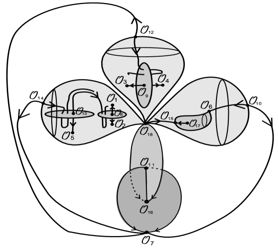
Figure 1: Phase portrait of a Morse-Smale diffeomorphism $f:\mathbb{S}^{3}\to\mathbb{S}^{3}$ with dynamical numbering of the periodic orbits

Definition 5

Let $\mathcal{O}_{1},\dots,\mathcal{O}_{k_{f}}$ be a dynamical numbering of the periodic orbits of $f$. A Morse-Lyapunov function $\varphi$ for $f$ is said to be dynamically ordered when $\varphi(\mathcal{O}_{i})=i$ for $i\in\{1,\dots,k_{f}\}$.

For each $i=1,\dots,k_{1}$, set $A_{i}=\bigcup\limits_{j=1}^{i}W^{u}_{\mathcal{O}_{j}}$. It is known that the set $A_{i}$ is an attractor, that is it has a trapping neighborhood $M_{i}$, which is a compact set such that $f(M_{i})\subset int\leavevmode\nobreak\ M_{i}$ ($M_{i}$ is $f$-compressed) and $\bigcap\limits_{k\geq 0}f^{k}(M_{i})=A_{i}$ (see, for example, [10]). Denote by $r_{i}$ the number of saddles, by $s_{i}$ the number of sinks and by $c_{i}$ the number of connected components in $A_{i}$. Set $g_{i}=c_{i}+r_{i}-s_{i}$.

Let us recall that a smooth compact orientable three-dimensional manifold is called a handlebody of a genus $g\geq 0$ if it is diffeomorphic to a manifold which is obtained from a closed 3-ball by an orientation reversing identification of $g$ pairs of pairwise disjoint closed 2-discs in its boundary. The boundary of such a handlebody is an orientable surface of genus $g$.

Definition 6

A trapping neighborhood $M_{i}$ of the attractor $A_{i}$ is called a handle if: $M_{i}$ consists of $c_{i}$ handlebodies. The sum $g_{{}_{M_{i}}}$ of genera of all connected components of $M_{i}$ is called genus of the handle neighborhood.

Notice that for each $i=1,\dots,k_{0}$, the number $g_{i}$ equals $0$, the attractor $A_{i}$ is zero-dimensional (as it consists of the sink orbits) and has a handle neighborhood $M_{i}$ of genus $g_{i}=0$ consisting of $c_{i}$ pairwise disjoint 3-balls (it follows, for example, from statement 6 below). For each $i=k_{0}+1,\dots,k_{1}$ the attractor $A_{i}$ contains an one-dimensional connected component, therefor we will say (taking liberty) that $A_{i}$ is one-dimensional attractor.

Proposition 1

Each one-dimensional attractor $A_{i}$ of Morse-Smale diffeomorphism $f:M\to M$ has a handle trapping neighborhood $M_{i}$ with genus $g_{{}_{M_{i}}}\geq g_{i}$.

Definition 7

A handle neighborhood $M_{i}$ of one-dimensional attractor $A_{i}$ is said to be tight if:

1) $g_{{}_{M_{i}}}=g_{i}$;

2) $W^{s}_{\sigma}\cap M_{i}$ consists of exactly one two-dimensional closed disc for each saddle point $\sigma\in\mathcal{O}_{i}$.

A one-dimensional attractor $A_{i}$ possessing tight trapping neighborhood $M_{i}$ is said to be tightly embedded.

By definition a repeller for $f$ is an attractor for $f^{-1}$. Moreover, dynamical numbering of the orbits $\mathcal{O}_{1},\dots,\mathcal{O}_{k_{f}}$ of a diffeomorphism $f$ induces a dynamical numbering of the orbits $\tilde{\mathcal{O}}_{1},\dots,\tilde{\mathcal{O}}_{k_{f}}$ of a diffeomorphism $f^{-1}$ next way: $\tilde{\mathcal{O}}_{i}=\mathcal{O}_{k_{f}-i}$. Then a one-dimensional repeller for $f$ is said to be tightly embedded if it is such an attractor for $f^{-1}$ according to induced numbering.

Notice that the property for a one-dimensional attractor (repeller) to be tightly embedded gives a topological information about the embedding of the unstable manifolds of its saddle periodic points. In the example which was constructed by D. Pixton in [9] the unique one-dimensional attractor $A_{3}=cl\,W^{u}_{\sigma}$ has the following property: $g_{3}=0$ but any 3-ball around $cl\,W^{u}_{\sigma}$ intersects $W^{s}_{\sigma}$ at more than one 2-disc (see figure 2, where are drawn the phase portrait of Pixton’s diffeomorpfism $f$ and a 3-ball). Hence, this one-dimensional attractor is not tightly embedded.

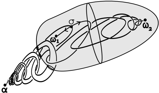
Figure 2: One-dimensional attractor of Pixton’s example is not tightly embedded

Our main results are the following theorems.

Theorem 1

If a Morse-Smale diffeomorphism $f:M\to M$ possesses a dynamically ordered energy function, then all one-dimensional attractors and repellers of $f$ are tightly embedded.

Definition 8

A tight trapping neighborhood $M_{i}$ of a one-dimensional attractor $A_{i}$ is called strongly tight if $M_{i}\setminus A_{i}$ is diffeomorphic to $\partial M_{i}\times(0,1]$. A one-dimensional attractor $A_{i}$ possessing a strongly tight trapping neighborhood $M_{i}$ is said to be strongly tightly embedded.

Theorem 2

Let $f$ be a Morse-Smale diffeomorphism on a closed 3-manifold $M$. If all one-dimensional attractors and repellers of $f$ are strongly tightly embedded, then $f$ possesses a dynamically ordered energy function.

Notice that the condition in the last theorem is not necessary. For example in section 5 of paper [4] there was constructed a diffeomorphism on $\mathbb{S}^{2}\times\mathbb{S}^{1}$ possessing a dynamically ordered energy function, but whose one-dimensional attractor and repeller are not strongly tightly embedded.

The next theorem states a criterion for the existence of some dynamically ordered energy function for a Morse-Smale diffeomorphism without heteroclinic curves given on $\mathbb{S}^{3}$. Methods from [1] for realizing Morse-Smale diffeomorphisms show that this class is not empty. Moreover, it contains diffeomorphisms with chains of intersections of saddle invariant manifolds of arbitrary length (see figure 3, where it is represented a phase portrait of a diffeomorphism from the class under consideration). The criterion is based on paper [2], where it is specified interrelation between topology of the ambient 3-manifold $M$ and structure of the non-wandering set of a Morse-Smale diffeomorphism without heteroclinic curves given on $M$. In particular, for any diffeomorphism of $\mathbb{S}^{3}$ without heteroclinic curves, the number $r$ of all saddles and the number $l$ of all sinks and sources satisfy the equality $r=l-2$ (see statement 7 below). This equality implies that $g_{i}=0$ for any one-dimensional attractor $A_{i}$. Thus, tightly embedded attractor $A_{i}$ is strong tightly embedded. Applying results of theorems 1, 2 we get next criterion.

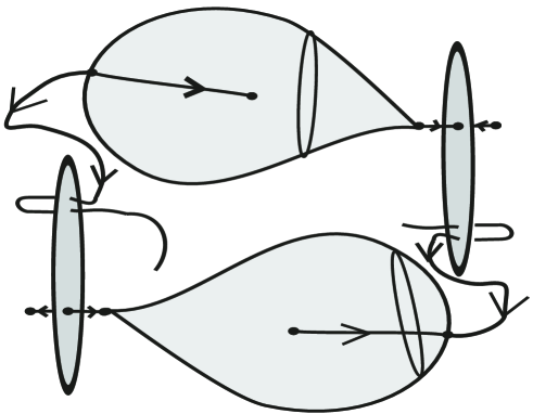
Figure 3: A Morse-Smale diffeomorphism without heteroclinic curves given on $\mathbb{S}^{3}$

Theorem 3

A Morse-Smale diffeomorphism $f:\mathbb{S}^{3}\to\mathbb{S}^{3}$ without heteroclinic curves possesses a dynamically ordered energy function if and only if each one-dimensional attractor and repeller is tightly embedded.

ACKNOWLEDGMENTS

V. Z. Grines and O. V. Pochinka acknowledge the support of the grant of government of Russian Federation no. 11.G34.31.0039 for partial financial support. F. Laudenbach is supported by the French program ANR “Floer power”.

2 Auxiliary facts

In this section, we recall some statements that we need in the proof and give references.

Statement 1

($\lambda$-lemma, [8]). Let $p$ be a hyperbolic fixed point of a diffeomorphism $f:M^{n}\to M^{n}$, $\dim W^{u}_{p}=\ell$, $0<\ell<n$, Let $B^{u}\subset W^{u}_{p}$ and $B^{s}\subset W^{s}_{p}$ be small $\ell$-disc and $(n-\ell)$-disc respectively centered at $p$. Let $V:=B^{u}\times B^{s}$ be their product in a chart about $p$. Let $B$ be an $\ell$-disc transverse to $W^{s}_{p}$ at $x$. Then, for any $\varepsilon>0$, there exists a positive integer $k_{0}$ such that the connected component of $f^{k}(B)\cap V$ containing $f^{k}(x)$ is $\varepsilon$-$C^{1}$-close to $B_{u}$ for each $k\geq k_{0}$.

Definition 9

Let $F$ be a compact smooth surface properly embedded in a 3-manifold $W$ (that is, $\partial F\subset\partial W$). Then $F$ is called compressible in one from two following cases:

1) there is a non contractible simple closed curve $c\subset int\leavevmode\nobreak\ F$ and smoothly embedded 2-disk $D\subset int\leavevmode\nobreak\ W$ such that $D\cap F=\partial D=c$;

2) there is a 3-ball $B\subset int\leavevmode\nobreak\ W$ such that $F=\partial B$.

The surface $F$ is said to be incompressible in $W$ if it is not compressible in $W$.

Statement 2

([13], corollary 3.2) Let $S_{g}$ be an orientable surface of genus $g\geq 1$ and let $F$ be an incompressible orientable surface properly embedded in $S_{g}\times[0,1]$ such that $\partial F\subset S_{g}\times\{1\}$. Then there is a surface $F_{1}\subset S_{g}\times\{1\}$ which is homeomorphic to $F$, such that $\partial F=\partial F_{1}$ and $F\cup F_{1}$ bounds domain $\Delta$ in $S_{g}\times[0,1]$ such that $cl\Delta$ is homeomorphic to $F\times[0,1]$, where $cl(\cdot)$ stands for the closure.

A particular case of statement 2 is the following fact.

Corollary 1

([5], theorem 3.3) Let $S_{g}$ be a closed orientable surface of genus $g\geq 1$ and let surface $F\subset int(S_{g}\times[0,1])$ be a closed surface which has genus $g$ and does not bound a domain in $S_{g}\times[0,1]$. Then $F$ is incompressible in $S_{g}\times[0,1]$ and the closure of each connected component of $S_{g}\times[0,1]\setminus F$ is homeomorphic to $S_{g}\times[0,1]$.

Proof: According to the preceding statement, it is sufficient to check that $F$ is incompressible in $S_{g}\times[0,1]$. If $F$ is compressible, there exists some incompressible surface $F^{\prime}$ whose genus $g^{\prime}$ is less than $g$ and which still does not bound a domain in $S_{g}\times[0,1]$. So $F^{\prime}$ is not a sphere and $g^{\prime}>0$. As $F^{\prime}$ is incompressible, the preceding statement tells us that $F^{\prime}$ is diffeomorphic to $S_{g}$. Contradiction. $\diamond$

Statement 3

([4], lemma 3.3) For any Morse-Smale diffeomorphism $f:M\to M$ we have that $1+|\Omega_{1}|-|\Omega_{0}|=1+|\Omega_{2}|-|\Omega_{3}|$, where $|\cdot|$ stands for the cardinality.

Statement 4

([7], theorem 5.2) Let $M^{n}$ be a closed manifold, $\varphi:M^{n}\to\mathbb{R}$ be a Morse function, $C_{q}$ be the number of all its critical points with index $q$, $\beta_{q}(M^{n})$ be the $q$-th Betti number and $\chi(M^{n})$ be the Euler characteristic. Then $\beta_{q}(M^{n})\leq C_{q}$ and $\chi(M^{n})=\sum\limits_{q=0}^{n}(-1)^{q}C_{q}$.

Statement 5

Let $\varphi:M^{n}\to\mathbb{R}$ be a Lyapunov function for a Morse-Smale diffeomorphism $f:M^{n}\to M^{n}$. Then

1) $-\varphi$ is Lyapunov function for $f^{-1}$;

2) if $p$ is a periodic point of $f$ then $\varphi(x)<\varphi(p)$ for every $x\in W^{u}_{p}\setminus p$ and $\varphi(x)>\varphi(p)$ for every $x\in W^{s}_{p}\setminus p$;

3) if $p$ is a periodic point of $f$ then $p$ is a critical point of $\varphi$ whose index is $\dim W^{u}_{p}$.

Statement 6

([4], lemma 2.2) Let $f:M^{n}\to M^{n}$ be a Morse-Smale diffeomorphism on an $n$-dimensional manifold and let $\mathcal{O}$ be a periodic orbit. For $p\in\mathcal{O}$, set $q=\dim W^{u}_{p}$. Then, there is some neighborhood $U$ and an energy function $\varphi:U\to\mathbb{R}$ for $f$ such that $(W^{u}_{p}\cap U)\subset Ox_{1}\dots x_{q},\leavevmode\nobreak\ (W^{s}_{p}\cap U)\subset Ox_{q+1}\dots x_{n}$ for Morse coordinates $x_{1},\dots,x_{n}$ of $\varphi$ near $p$.

Statement 7

([2], theorem) Let $M$ be a three-dimensional closed, connected, orientable manifold. Let $f:M\to M$ be any Morse-Smale diffeomorphism without heteroclinic curves whose non-wandering set consists of $r$ saddles and $l$ nodes (sinks and sources). Then $m=\frac{r-l+2}{2}$ is non negative integer and following facts hold:

1) if $m=0$, then $M$ is the 3-sphere;

2) if $m>0$, then $M$ is the connected sum of $m$ copies $\mathbb{S}^{2}\times\mathbb{S}^{1}$.

Conversely, for any non negative integers $r,l,m$ such that $m=\frac{r-l+2}{2}$ is non negative integer, there exists 3-manifold $M$ and some Morse-Smale diffeomorphism $f:M\to M$ with following properties:

a) $M$ is 3-sphere if $m=0$ and $M$ is the connected sum of $m$ copies $\mathbb{S}^{2}\times\mathbb{S}^{1}$ if $m>0$;

b) the non-wandering set of $f$ consists of $r$ saddles and $l$ sinks and sources, the wandering set of $f$ has no heteroclinic curves.

3 On one-dimensional attractors

Proof of proposition 1

For each $i=k_{0}+1,\dots,k_{1}$ let us prove the existence of handle neighborhood $M_{i}$ for one-dimensional attractor $A_{i}$ with $g_{{}_{M_{i}}}\geq g_{i}$.

Proof: According to statement 6, there is a neighborhood $U_{A_{k_{0}}}\subset W^{s}_{A_{k_{0}}}$ of zero-dimensional attractor $A_{k_{0}}$ and an energy function $\varphi_{A_{k_{0}}}:U_{A_{k_{0}}}\to\mathbb{R}$ for $f$ such that $\varphi_{A_{k_{0}}}(A_{k_{0}})=0$ and for small $\varepsilon>0$ each connected component of set $M_{k_{0}}=\varphi^{-1}_{A_{k_{0}}}((-\infty,\varepsilon])$ reads $\{(x_{1},x_{2},x_{3})\in U_{A_{k_{0}}}\leavevmode\nobreak\ :\leavevmode\nobreak\ x^{2}_{1}+x^{2}_{2}+x^{2}_{3}\leq\varepsilon\}$ in local coordinates $x_{1},x_{2},x_{3}$. Then $M_{k_{0}}$ is trapping neighborhood of zero-dimensional attractor $A_{k_{0}}$, which is a union of $c_{k_{0}}$ pairwise disjoint 3-balls. By induction on $i=k_{0}+1,\dots,k_{1}$ we construct a handle trapping neighborhood $M_{i}$ for $A_{i}$.

Let $i=k_{0}+1$. Set $S_{k_{0}}=\partial M_{k_{0}}$. Without loss of generality we can suppose that $S_{k_{0}}$ intersects $W^{u}_{\mathcal{O}_{k_{0}+1}}$ transversely; let $n_{k_{0}}$ be the number of intersection points. Set $V_{k_{0}}=W^{s}_{\Omega_{f}\cap A_{k_{0}}}\setminus A_{k_{0}}.$ Then the quotient $\hat{V}_{k_{0}}=V_{k_{0}}/f$ is made of the cobordism $M_{k_{0}}\setminus int\,f(M_{k_{0}})$ by gluing its boundaries by $f$. Hence, $\hat{V}_{k_{0}}$ is smooth orientable 3-manifold without boundary and natural projection $p_{{}_{k_{0}}}:V_{k_{0}}\to\hat{V}_{k_{0}}$ is cover. Then $p_{{}_{k_{0}}}(W^{u}_{\mathcal{O}_{k_{0}+1}})$ is a pair of knots which intersects $p_{{}_{k_{0}}}(S_{k_{0}})$ transversely at $n_{k_{0}}$ points. Thus, there is a tubular neighborhood $\hat{T}^{u}_{k_{0}+1}\subset\hat{V}_{k_{0}}$ of $p_{{}_{k_{0}}}(W^{u}_{\mathcal{O}_{k_{0}+1}})$ such that $\hat{T}^{u}_{k_{0}+1}\cap p_{{}_{k_{0}}}(S_{k_{0}})$ consists of $n_{k_{0}}$ 2-discs.

Figure 4: Construction of a handle neighborhood for one-dimensional attractor

Set $T^{u}_{k_{0}+1}=p^{-1}_{k_{0}}(\hat{T}^{u}_{k_{0}+1})$. According to the $\lambda$-lemma (see statement 1), $T^{u}_{k_{0}+1}\cup W^{s}_{\mathcal{O}_{k_{0}+1}}$ is a neighborhood of $\mathcal{O}_{k_{0}+1}$. According to statement 6, there are some neighborhood $U_{\mathcal{O}_{k_{0}+1}}\subset(T^{u}_{k_{0}+1}\cup W^{s}_{\mathcal{O}_{k_{0}+1}})$ of $\mathcal{O}_{k_{0}+1}$ and an energy function $\varphi_{\mathcal{O}_{k_{0}+1}}:U_{\mathcal{O}_{k_{0}+1}}\to\mathbb{R}$ for $f$ with $\varphi_{\mathcal{O}_{k_{0}+1}}(\mathcal{O}_{k_{0}+1})=0$. When $\varepsilon>0$ is small enough, each connected component of $H_{k_{0}+1}=\varphi^{-1}_{\mathcal{O}_{k_{0}+1}}((-\infty,\varepsilon])$ reads $\{(x_{1},x_{2},x_{3})\in U_{\mathcal{O}_{k_{0}+1}}\leavevmode\nobreak\ :\leavevmode\nobreak\ -x^{2}_{1}+x^{2}_{2}+x^{2}_{3}\leq\varepsilon\}$ in local coordinates $x_{1},x_{2},x_{3}$. According to the $\lambda$-lemma, when $k\in\mathbb{N}$ is large enough, $f^{-k}(S_{k_{0}})$ intersects both $H_{k_{0}+1}$ and $f(H_{k_{0}+1})$, its intersection with these domains consists of $n_{k_{0}}$ 2-discs and $f(H_{k_{0}+1})\setminus int\,f^{-k}(M_{k_{0}})\subset int\,H_{i}$ (see figure 4). Thus, $M_{k_{0}+1}=f^{-k}(M_{k_{0}})\cup H_{k_{0}+1}$ is a union of handlebodies, as it is obtained from the union of 3-balls $f^{-k}(M_{k_{0}})$ by gluing one-handles $H_{k_{0}+1}\setminus int\,f^{-k}(M_{k_{0}})$. Let us show that $f(M_{k_{0}+1})\subset int\,M_{k_{0}+1}$.

Indeed, it is true for a point $x\in f^{-k}(M_{k_{0}})$ as $f^{-k}(M_{k_{0}})$ is $f$-compressed and it is true for a point $x\in(H_{k_{0}+1}\setminus f^{-k}(M_{k_{0}}))$ as $f(H_{k_{0}+1})\setminus int\,f^{-k}(M_{k_{0}})\subset int\,H_{k_{0}+1}$.

Let us prove the equality $\bigcap\limits_{k\geq 0}f^{k}(M_{k_{0}+1})=A_{k_{0}+1}$. As $A_{k_{0}+1}\subset M_{k_{0}+1}$ and $f^{k}(A_{k_{0}+1})=A_{k_{0}+1}$ for $k\in\mathbb{Z}$ then $A_{k_{0}+1}\subset\bigcap\limits_{k\geq 0}f^{k}(M_{k_{0}+1})$. Let us set $A^{\prime}_{k_{0}+1}=\bigcap\limits_{k\geq 0}f^{k}(M_{k_{0}+1})$ and show that $A^{\prime}_{k_{0}+1}=A_{k_{0}+1}$. Assume contrary: there is a point $x\in(A^{\prime}_{k_{0}+1}\setminus A_{k_{0}+1})$. Due to theorem 2.3 in [11] there is a point $p\in(\Omega_{f}\setminus A_{k_{0}+1})$ such that $x\in W^{u}_{p}$. As the set $A^{\prime}_{k_{0}+1}$ is closed and invariant then $cl\leavevmode\nobreak\ (\mathcal{O}_{x})\subset A^{\prime}_{k_{0}+1}$ and, hence, $p\in A^{\prime}_{k_{0}+1}$. This is a contradiction with the fact $A^{\prime}_{k_{0}+1}\subset W^{s}_{A_{k_{0}+1}\cap\Omega_{f}}$.

Recall that we denote by $r_{i}$ the number of saddles, by $s_{i}$ the number of sinks, by $c_{i}$ the number of connected components of the attractor $A_{i}$ and set $g_{i}=c_{i}+r_{i}-s_{i}$. By the construction $M_{k_{0}+1}$ consists of $c_{k_{0}+1}$ 3-balls with 1-handles. Denote by $g_{{}_{M_{k_{0}+1}}}$ the sum of genera of connected components of $M_{k_{0}+1}$. Let us show that $g_{{}_{M_{k_{0}+1}}}\geq g_{k_{0}+1}$.

In denotation above, the number of points in the orbit $\mathcal{O}_{{k_{0}+1}}$ equals $r_{{k_{0}+1}}-r_{k_{0}}$. As $A_{{k_{0}+1}}=A_{k_{0}}\cup W^{u}_{\mathcal{O}_{{k_{0}+1}}}$ and $cl\leavevmode\nobreak\ W^{u}_{\mathcal{O}_{{k_{0}+1}}}\setminus W^{u}_{\mathcal{O}_{{k_{0}+1}}}\subset A_{k_{0}}$ then $c_{{k_{0}+1}}\leq c_{k_{0}}$. Denote by $l_{k_{0}+1}$ the number of connected components of the set $H_{{k_{0}+1}}\setminus int\,f^{-k}(M_{k_{0}})$. By the construction each of them is 1-handle and removing of $(l_{{k_{0}+1}}-(c_{k_{0}}-c_{{k_{0}+1}}))$ 1-handles from $M_{k_{0}+1}$ gives the set with the same $c_{k_{0}+1}$ connected components. Then the sum of genera $g_{{}_{M_{k_{0}}}}$ of $M_{k_{0}}$ can be calculate by formula $g_{{}_{M_{k_{0}}}}=g_{{}_{M_{k_{0}+1}}}-(l_{{k_{0}+1}}-(c_{k_{0}}-c_{{k_{0}+1}}))$. By the construction $l_{k_{0}+1}\geq(r_{{k_{0}+1}}-r_{k_{0}})$, hence $g_{{}_{M_{k_{0}}}}\leq g_{{}_{M_{k_{0}+1}}}-(r_{{k_{0}+1}}-r_{k_{0}}-(c_{k_{0}}-c_{{k_{0}+1}}))$ and $g_{{}_{M_{k_{0}+1}}}\geq g_{{}_{M_{k_{0}}}}+r_{{k_{0}+1}}-r_{k_{0}}-c_{k_{0}}+c_{{k_{0}+1}}$. As $g_{{}_{M_{k_{0}}}}=g_{k_{0}}$ then $g_{{}_{M_{k_{0}+1}}}\geq c_{k_{0}}+r_{k_{0}}-s_{k_{0}}+r_{{k_{0}+1}}-r_{k_{0}}-c_{k_{0}}+c_{{k_{0}+1}}=c_{{k_{0}+1}}+r_{{k_{0}+1}}-s_{k_{0}}$. As $s_{k_{0}}=s_{k_{0}+1}$ then $g_{{}_{M_{k_{0}+1}}}\geq g_{k_{0}+1}$.

A smoothing of the set $M_{k_{0}+1}$ is the required handle trapping neighborhood.

Assuming that handle neighborhood for attractor $A_{i-1}$ already constructed, repeating construction above (changing $k_{0}$ by $i-1$), we construct $f$-compressed set $M_{i}=f^{-k}(M_{i-1})\cup H_{i}$, being a union of handle neighborhood $f^{-k}(M_{i-1})$ with 1-handles $H_{i}\setminus int\,f^{-k}(M_{i-1})$. It is similar proved that $M_{i}$ is required handle neighborhood. $\diamond$

Proposition 2

The one-dimensional attractor $A_{k_{1}}$ is connected.

Proof: Firstly, let us prove that any trapping neighborhood $M_{k_{1}}$ of $A_{k_{1}}$ is connected. Let us assume the contrary: $M_{k_{1}}$ is a union of pairwise disjoint closed sets $B_{1}$ and $B_{2}$. As $M_{k_{1}}$ is $f$-compressed then without loss of generality we can suppose that $f(B_{i})\subset int\,B_{i},\leavevmode\nobreak\ i=1,2$. By construction, $U_{1}=\bigcup\limits_{k>0}f^{-k}(int\,B_{1})$, $U_{2}=\bigcup\limits_{k>0}f^{-k}(int\,B_{2})$ are pairwise disjoint open sets and $U_{1}\cup U_{2}=W^{s}_{\Omega_{0}\cup\Omega_{1}}$. On the other hand $W^{s}_{\Omega_{0}\cup\Omega_{1}}=M\setminus W^{s}_{\Omega_{2}\cup\Omega_{3}}$ and, hence, $W^{s}_{\Omega_{0}\cup\Omega_{1}}$ is connected as $\dim\,M=3$ and $\dim\,W^{s}_{\Omega_{2}\cup\Omega_{3}}\leq 1$. This is a contradiction.

Thus $A_{i}$ is connected as intersection of nested connected compact sets $M_{i}\supset f(M_{i})\supset\dots\supset f^{k}(M_{i})\supset\dots$. $\diamond$

4 Necessary condition for existence of dynamically ordered energy function

Proof of theorem 1

Let us prove that if a Morse-Smale diffeomorphism $f:M\to M$ has a dynamically ordered energy function, then its one-dimensional attractors and repellers are tightly embedded.

Proof: Notice that $f$ and $f^{-1}$ possess dynamically ordered energy functions simultaneously. Indeed, if $\varphi:M\to\mathbb{R}$ is such function for $f$ then $-\varphi:M\to\mathbb{R}$ is an energy function for $f^{-1}$ (see statement 5) and $\tilde{\varphi}=k_{f}+1-\varphi:M\to\mathbb{R}$ is dynamically ordered energy function for $f^{-1}$. Therefore, it is enough to prove the fact for attractors.

Let $\varphi:M\to\mathbb{R}$ be a dynamically ordered energy function for $f:M\to M$, $i=k_{0}+1,\dots,k_{1}$ and $M_{i}=\varphi^{-1}([1,i+\varepsilon_{i}]),\varepsilon_{i}>0$. It follows from properties of dynamically ordered energy function and statement 5 that any orbit $\mathcal{O}_{j}$ with number $j\leq i$ belongs to $M_{i}$. Due to statement 5, $W^{u}_{\mathcal{O}_{j}}\subset M_{i}$. Thus $A_{i}\subset M_{i}$. It follows from definition of Lyapunov function that $f(M_{i})\subset int\leavevmode\nobreak\ M_{i}$. Similar to proposition 1 it is proved equality $\bigcap\limits_{k\geq 0}f^{k}(M_{i})=A_{i}$. Thus, $M_{i}$ is trapping neighborhood of attractor $A_{i}$. Then $M_{i}$ has the same number of connected components as $A_{i}$. Let us prove that there is $\varepsilon_{i}>0$ such that $M_{i}$ is a tight neighborhood of $A_{i}$.

As $\varphi$ is a Morse-Lyapunov function then there is $\varepsilon_{i}>0$ such that $W^{s}_{\sigma}\cap M_{i}$ consists of exactly one closed 2-disc for each saddle point $\sigma\in\mathcal{O}_{i}$. It follows from properties of dynamically ordered energy function and statement 5 that $\varphi|_{M_{i}}$ has exactly $r_{i}+s_{i}$ critical points, among of them $s_{i}$ points have index $0$ and $r_{i}$ points have index $1$. According to Morse theory, $M_{i}$ is a union of of $s_{i}$ 3-balls with gluing of $r_{i}$ 1-handles and hence is a union of $c_{i}$ handlebodies. Denote by $g_{{}_{M_{i}}}$ the sum of genus of handlebodies from $M_{i}$. According to statement 4, $\chi(M_{i})=s_{i}-r_{i}$. It follows from Morse theory that $M_{i}$ has the homotopy type of a cellular complex consisting of $s_{i}$ zero-dimensional and $r_{i}$ one-dimensional cells, then $-g_{{}_{M_{i}}}+c_{i}=m_{i}-r_{i}$ or $g_{{}_{M_{i}}}=g_{i}$. $\diamond$

5 Construction of a dynamically ordered energy function for $f$

Now $f$ is a Morse-Smale diffeomorphism on a closed 3-manifold $M$ and its one-dimensional attractors and repellers are strongly tightly embedded. Construction of a dynamically ordered energy function for $f$ is based on technical lemmas of next section.

Recall that, by assumption of theorem 2, each one-dimensional attractor $A_{i},\leavevmode\nobreak\ i=k_{0}+1,\dots,k_{1}$ is strongly tightly embedded and, hence, has a handle neighborhood $M_{i}$ of genus $g_{i}$ such that $M_{i}\setminus A_{i}$ is homeomorphic to $S_{i}\times(0,1]$, where $S_{i}=\partial M_{i}$, and for each point $\sigma\in\mathcal{O}_{i}$ the intersection $W^{s}_{\sigma}\cap M_{i}$ consists of exactly one 2-disk. Set $D_{i}=M_{i}\cap W^{s}_{\mathcal{O}_{i}}$. According to statement 6, for each zero-dimensional attractor $A_{i},\leavevmode\nobreak\ i=1,\dots,k_{0}$, there is a handle neighborhood of genus $g_{i}=0$ which is a union of $c_{i}$ 3-balls, we will denote it by $M_{i}$ and set $S_{i}=\partial M_{i}$.

For $i=1,\dots,k_{1}$ set $K_{i}=M_{i}\setminus int\leavevmode\nobreak\ f(M_{i})$, $N_{i}=W^{s}_{A_{i}\cap\Omega_{f}}$ and $V_{i}=N_{i}\setminus A_{i}$. According to ring hypothesis and corollary 1, $K_{i}$ is diffeomorphic to $S_{i}\times[0,1]$. As $V_{i}=\bigcup\limits_{n\in\mathbb{Z}}f^{n}(K_{i})$ then $V_{i}$ is diffeomorphic to $S_{i}\times\mathbb{R}$.

5.1 Extension of Lyapunov functions

Definition 10

Let $D$ be a subset of $M$ which is diffeomorphic to product $S\times[0,1]$ for some (possibly non connected) surface $S$. Then $D$ is said to be an $(f,S)$-compressed product when there is a diffeomorphism $g:D\to S\times[0,1]$ such that $g^{-1}(S\times\{t\})$ bounds an $f$-compressed domain in $M$ for any $t\in[0,1]$.

Proposition 3

Let $D$ be an $(f,S)$-compressed product. Then for any values $d_{0}<d_{1}$ there is an energy function $\varphi_{{}_{D}}:D\to\mathbb{R}$ for $f|_{D}$ such that $\varphi_{{}_{D}}(g^{-1}(S\times\{0\}))=d_{0}$ and $\varphi_{{}_{D}}(g^{-1}(S\times\{1\}))=d_{1}$.

Proof: The desired function $\varphi_{{}_{D}}:D\to\mathbb{R}$ is defined by formula $\varphi_{{}_{D}}(x)=d_{0}+t(d_{1}-d_{0})$ for $x\in g^{-1}(S\times\{t\}),\leavevmode\nobreak\ t\in[0,1]$. $\diamond$

Lemma 1

Let $i\in\{1,\dots,k_{1}\}$ and $P_{i}$, $Q_{i}$ be handle neighborhoods of genus $g_{i}$ of the attractor $A_{i}$. If there is a dynamically ordered energy function $\varphi_{{}_{Q_{i}}}:Q_{i}\to\mathbb{R}$ for $f$ with $S_{Q_{i}}=\partial Q_{i}$ as a level set then there is a dynamically ordered energy function $\varphi_{{}_{P_{i}}}:P_{i}\to\mathbb{R}$ for $f$ with $S_{P_{i}}=\partial P_{i}$ as a level set.

Proof: We follow to scheme of the proof of lemma 4.2 from [3]. Give some remarks.

Without loss of generality we assume that $Q_{i}\subset int\leavevmode\nobreak\ P_{i}$ (in the opposite case, instead pair $(Q_{i},\varphi_{{}_{Q_{i}}})$ we can use pair $(f^{n}(Q_{i}),\varphi_{{}_{f^{n}(Q_{i})}})$, where $f^{n}(Q_{i})\subset int\leavevmode\nobreak\ P_{i}$ and $\varphi_{{}_{f^{n}(Q_{i})}}=\varphi_{{}_{Q_{i}}}f^{-n}$). As $V_{i}$ is diffeomorphic to $S_{i}\times\mathbb{R}$ then, according to ring hypothesis and corollary 1, $G_{i}={P}_{i}\setminus int\,{Q}_{i}$ is a product. As handle neighborhoods $f^{n}(Q_{i})$ and $f^{n}(P_{i})$ contain the attractor $A_{i}$ for each $n\in\mathbb{Z}$ then the surfaces $f^{n}(S_{Q_{i}})$ and $f^{n}(S_{P_{i}})$ do not bound domains in $V_{i}$ and, hence, are incompressible due to corollary 1. Now let us construct the function $\varphi_{{}_{P_{i}}}$, for this aim we consider two cases: 1) $S_{P_{i}}\cap(\bigcup\limits_{n>0}f^{-n}({S_{Q_{i}}}))=\emptyset$ and 2) $S_{P_{i}}\cap(\bigcup\limits_{n>0}f^{-n}({S_{Q_{i}}}))\neq\emptyset$.

In case 1), let $m$ be the first positive integer such that $f^{m}({P_{i}})\subset int\,{Q}_{i}$. If $m=1$, then $G_{i}$ is $(f,S_{i})$-compressed product and proposition 3 yields the required function as extension of the function $\varphi_{{}_{Q_{i}}}$ to $G_{i}$.

If $m>1$, the surfaces $f({S}_{P_{i}}),f^{2}({S}_{P_{i}}),\dots,f^{m-1}({S}_{P_{i}})$ are mutually “parallel”, that is: two by two they bound a product cobordism (according to ring hypothesis and corollary 1). Therefore they subdivide $G_{i}$ in $(f,S_{i})$-compressed products and, hence, proposition 3 yields the required function as extension of the function $\varphi_{{}_{Q_{i}}}$ to $f^{m-1}(P_{i})\setminus int\leavevmode\nobreak\ Q_{i},f^{m-2}(P_{i})\setminus int\leavevmode\nobreak\ f^{m-1}(P_{i}),\dots,P_{i}\setminus int\leavevmode\nobreak\ f(P_{i})$ in series.

In case 2), without loss of generality we may assume that $S_{P_{i}}$ is transverse to $\bigcup\limits_{n>0}f^{-n}({S}_{Q_{i}})$, which implies that there is a finite family $\mathcal{C}$ of intersection curves. We are going to describe a process of decreasing the number of intersection curves by an isotopy of ${Q}_{i}$ among handle neighborhoods of genus $g_{i}$ possessing a dynamically ordered energy function for $f$ which is constant on the boundary of the neighborhood.

Firstly we consider all intersection curves from $\mathcal{C}$ which are homotopic to zero in $S_{P_{i}}$. Let $c$ be an innermost such curve. Then there is a disc $\delta\subset S_{P_{i}}$ which is bounded by $c$ and such that $int\,\delta$ contains no curves from the family $\mathcal{C}$. As $c\subset f^{-n}(S_{Q_{i}})$ for some $n$ and $f^{-n}(S_{Q_{i}})$ is incompressible in $V_{i}$, then $c$ bounds a disc $d\subset f^{-n}(S_{Q_{i}})$. Then 2-sphere $\delta\cup d$ is embedded and bounds a 3-ball $b$ in $N_{i}$ (when the component of $f^{-n}(S_{Q_{i}})$ containing $d$ is a 2-sphere, replace $d$ by the complementary disc if necessary).

There are two occurrences: (a) $f^{n}(b)\subset Q_{i}$ and (b) $f^{n}(b)\subset f^{-1}(Q_{i})$. We define $Q_{i}^{\prime}$ as $cl(Q_{i}\setminus f^{n}(b))$ in the case (a) and $Q_{i}\cup f^{n}(b)$ in the case (b). The fact that $c$ is an innermost curve implies $f(Q_{i})\subset Q_{i}^{\prime}\subset Q_{i}$ in case (a) and $Q_{i}\subset Q_{i}^{\prime}\subset f^{-1}(Q_{i})$ in case (b). In both cases there is a smooth approximation $\tilde{Q}_{i}$ of $Q_{i}^{\prime}$ such that $f(Q_{i})\subset int\leavevmode\nobreak\ \tilde{Q}_{i}\subset Q_{i}$ if (a), $Q_{i}\subset int\leavevmode\nobreak\ \tilde{Q}_{i}\subset f^{-1}(Q_{i})$ if (b), and the number of intersection curves in $S_{P_{i}}\cap(\bigcup\limits_{n>0}f^{-n}(\partial\tilde{Q}_{i}))$ is less than the cardinality of $\mathcal{C}$.

In case (a), $\varphi_{{}_{f(Q_{i})}}=\varphi_{{}_{Q_{i}}}f^{-1}:f(Q_{i})\to\mathbb{R}$ is a dynamically ordered energy function which is constant on the boundary. Therefore $\tilde{Q}_{i}\setminus int\leavevmode\nobreak\ f(Q_{i})$ is an $(f,S_{i})$-compressed product and, hence, due to proposition 3, there is a similar function on $\tilde{Q}_{i}$. Similarly in case (b), $\tilde{Q}_{i}$ is equipped with a dynamically ordered energy function which is constant on the boundary as $\tilde{Q}_{i}\setminus int\leavevmode\nobreak\ Q_{i}$ is an $(f,S_{i})$-compressed product.

We will repeat this process until getting a handle neighborhood $\hat{Q}_{i}$ of genus $g_{i}$ for the attractor $A_{i}$ such that $S_{P_{i}}\cap(\bigcup\limits_{n>0}f^{-n}(\partial\hat{Q}_{i}))$ does not contain curves which are homotopic zero in $S_{P_{i}}$. Thus we may assume that $S_{P_{i}}\cap(\bigcup\limits_{n>0}f^{-n}({S_{Q_{i}}}))$ does not contain intersection curves which are homotopic to zero in $S_{P_{i}}$.

We denote by $m$ the largest integer such that $f^{m}(S_{P_{i}})\cap S_{Q_{i}}\neq\emptyset$. Let $F$ be a connected component of $f^{m}(S_{P_{i}})\cap G_{i}$. We have $\partial F\subset\partial{S}_{Q_{i}}$. Let us show that $F$ is incompressible in $G_{i}$. Indeed, if $\delta$ is a disc in $G_{i}$ with boundary $\gamma\subset F$ then $\gamma$ bounds 2-disk $\tilde{\delta}\subset f^{m}(S_{P_{i}})$ as $f^{m}(S_{P_{i}})$ is incompressible surface in $V_{i}$. By assumption the components of $\partial F$ are not homotopic to zero in $f^{m}(S_{P_{i}})$, then $\partial F\cap\tilde{\delta}=\emptyset$ and, hence, $\tilde{\delta}\subset F$.

Therefore, according to statement 2 there is some surface $F_{1}\subset S_{Q_{i}}$ diffeomorphic to $F$, with $\partial F=\partial F_{1}$, and $F\cup F_{1}$ bounds a domain $\Delta$ in $G_{i}$ which, up to smoothing of the boundary, is diffeomorphic to $F\times[0,1]$. We then define $\tilde{Q}_{i}$ as $Q_{i}\cup\Delta$ up to smoothing. By the choice of $m$, $\tilde{Q}_{i}$ is $f$-compessed as $f(\Delta)\subset Q_{i}$. As $\tilde{Q}_{i}$ is obtained by an isotopy supported in a neighborhood of $\Delta$ from $Q_{i}$ then $\tilde{Q}_{i}\setminus int\leavevmode\nobreak\ Q_{i}$ is an $(f,S_{i})$-compressed product. Thus we get a dynamically ordered energy function on $\tilde{Q}_{i}$ with $\partial\tilde{Q}_{i}$ as a level set. Arguing recursively, we are reduced to case 1). $\diamond$

Lemma 2

Let $i\in\{k_{0}+1,\dots,k_{1}\}$, $M_{i}$ be strongly tight neighborhood of the attractor $A_{i}$, $D_{i}=M_{i}\cap W^{s}_{\mathcal{O}_{i}}$ and $N(D_{i})\subset M_{i}$ be a tubular neighborhood of $D_{i}$ such that $N(D_{i})\cap A_{i-1}=\emptyset$ and the set $P_{i-1}=M_{i}\setminus int\leavevmode\nobreak\ N(D_{i})$ is $f$-compressed. Then $P_{i-1}$ is a handle neighborhood of genus $g_{i-1}$ for the attractor $A_{i-1}$.

Proof: Similar to proposition 1 it is proved the equality $\bigcap\limits_{k\geq 0}f^{k}(P_{i-1})=A_{i-1}$. Thus $P_{i-1}$ is a trapping neighborhood of the attractor $A_{i-1}$ and, hence, the set $P_{i-1}$ consists of $c_{i-1}$ connected components. Each of them is handlebody, as it is obtained from $M_{i}$ removing $(r_{i}-r_{i-1})$ 1-handles, which are the set $N(D_{i})$. As in proof of proposition 1, a sum $g_{{}_{P_{i-1}}}$ of genera $P_{i-1}$ is calculated by formula $g_{{}_{P_{i-1}}}=g_{i}-((r_{i}-r_{i-1})-(c_{i-1}-c_{i}))$. Then $g_{{}_{P_{i-1}}}=c_{i}+r_{i}-s_{i}-((r_{i}-r_{i-1})-(c_{i-1}-c_{i}))=c_{i-1}+r_{i-1}-s_{i}$. As $s_{i-1}=s_{i}$ then $g_{{}_{P_{i-1}}}=g_{i-1}$. $\diamond$

5.2 Global construction

We divide a construction of the dynamically ordered energy function for $f:M\to M$ on steps.

Step 1. By induction on $i=1,\dots,k_{1}$ let us prove the existence of a dynamically ordered energy function $\varphi_{{}_{M_{i}}}$ on $M_{i}$ of the attractor $A_{i}$ with level set $S_{i}$.

For $i=1$ the attractor $A_{1}$ coincides with sink orbit $\mathcal{O}_{1}$ of the diffeomorphism $f$. According to statement 6 there is a neighborhood $U_{\mathcal{O}_{1}}\subset M$ of the orbit $\mathcal{O}_{1}$, equipped by an energy function $\varphi_{\mathcal{O}_{1}}:U_{\mathcal{O}_{1}}\to\mathbb{R}$ for $f$ and such that $\varphi_{\mathcal{O}_{1}}(\mathcal{O}_{1})=1$. Moreover, for each connected component $U_{\omega}$, $\omega\in\mathcal{O}_{1}$ of the set $U_{\mathcal{O}_{1}}$ there are Morse coordinates $(x_{1},x_{2},x_{3})$ such that $\varphi_{\mathcal{O}_{1}}(x_{1},x_{2},x_{3})=1+x_{1}^{2}+x_{2}^{2}+x_{3}^{2}$. Then there is a value $\varepsilon_{1}>0$ such that set $Q_{1}=\varphi^{-1}_{\mathcal{O}_{1}}(1+\varepsilon_{1})$ consists of $f$-compressed union of $c_{1}$ 3-balls. Thus $Q_{1}$ is a handle neighborhood of genus $0$ for the attractor $A_{1}$. As $g_{1}=0$ then, according to lemma 1, there is a dynamically ordered energy function $\varphi_{{}_{M_{1}}}$ on the neighborhood $M_{1}$ for the attractor $A_{1}$ with level set $S_{1}$.

Let, by assumption of the induction, there is a dynamically ordered energy function $\varphi_{{}_{M_{i-1}}}$ on the neighborhood $M_{i-1}$ of the attractor $A_{i-1}$ with level set $S_{i-1}$. Let us construct the function $\varphi_{{}_{M_{i}}}$. There is two cases: a) $i\leq k_{0}$; b) $i>k_{0}$.

In the case a) the neighborhood $M_{i}$ consists of a handle neighborhood of genus $0$ for the attractor $A_{i-1}$ (denote it $P_{i-1}$) and a trapping neighborhood of the orbit $\mathcal{O}_{i}$, consisting from 3-balls (denote it $Q_{i}$). By assumption of the induction and lemma 1 there is a dynamically ordered energy function $\varphi_{{}_{P_{i-1}}}$ on $P_{i-1}$ with level set $\partial P_{i-1}$. Similar to case $i=1$ it is shown the existence of a dynamically ordered energy function $\varphi_{{}_{Q_{i}}}$ on $Q_{i}$ with level set $\partial Q_{i}$. The required function $\varphi_{{}_{M_{i}}}$ is formed from $\varphi_{{}_{P_{i-1}}}$ and $\varphi_{{}_{Q_{i}}}$.

b) we follow to scheme of proof from section 4.3 of paper [3].

According to statement 6, the orbit $\mathcal{O}_{i}$ has a neighborhood $U_{\mathcal{O}_{i}}\subset M$ endowed with an energy function $\varphi_{\mathcal{O}_{i}}:U_{\mathcal{O}_{i}}\to\mathbb{R}$ of $f$ with $\varphi_{\mathcal{O}_{i}}(\mathcal{O}_{i})=i$. Moreover, each connected component $U_{\sigma}$, $\sigma\in\mathcal{O}_{i}$ of $U_{\mathcal{O}_{i}}$ is endowed with Morse coordinates $(x_{1},x_{2},x_{3})$ such that $\varphi_{\mathcal{O}_{i}}(x_{1},x_{2},x_{3})=i+x_{1}^{2}+x_{2}^{2}+x_{3}^{2}$, the $x_{1}$-axis is contained in the unstable manifold and the $(x_{2},x_{3})$-plane is contained in the stable manifold of $\sigma$.

It follows from properties of strongly tight neighborhood $M_{i}$ and $\lambda$-lemma that there is a tubular neighborhood $N(D_{i})\subset M_{i}$ of $D_{i}=M_{i}\cap W^{s}_{\mathcal{O}_{i}}$ such that $N(D_{i})\cap A_{i-1}=\emptyset$, set $P_{i-1}=M_{i}\setminus int\leavevmode\nobreak\ N(D_{i})$ is $f$-compressed and surface $\partial P_{i-1}$ transversal intersects each connected component of the set $\varphi^{-1}_{\mathcal{O}_{i}}(i)\setminus\mathcal{O}_{i}$ at one closed curve. By lemma 2, the set $P_{i-1}$ is a handle neighborhood of genus $g_{i-1}$ for the attractor $A_{i-1}$. By assumption of induction and lemma 1 there is a dynamically ordered energy function $\varphi_{{}_{P_{i-1}}}$ on $P_{i-1}$ with level set $\partial P_{i-1}$.

For $\varepsilon_{i}\in(0,1),\leavevmode\nobreak\ t\in[-\varepsilon_{i},\varepsilon_{i}]$ set $P_{t}=\varphi^{-1}_{{P_{i-1}}}([1,\varphi_{{}_{P_{i-1}}}(\partial P_{i-1})-\varepsilon_{i}+t])$, $H_{t}=\{x\in U_{\mathcal{O}_{i}}\leavevmode\nobreak\ :\leavevmode\nobreak\ \varphi_{\mathcal{O}_{i}}(x)\leq i+{t}\}$ and $E_{\varepsilon_{i}}=(P_{\varepsilon_{i}}\setminus int\leavevmode\nobreak\ P_{-\varepsilon_{i}})\cap(H_{\varepsilon_{i}}\setminus int\leavevmode\nobreak\ H_{-\varepsilon_{i}})$ (see figure 5). Notice that $P_{\varepsilon_{i}}=P_{i-1}$ and, hence, $f(P_{\varepsilon_{i}})\subset int\leavevmode\nobreak\ P_{\varepsilon_{i}}$. As $\varphi_{\mathcal{O}_{i}}$ is a Lyapunov function for $f|_{U_{\mathcal{O}_{i}}}$ then $\varphi_{\mathcal{O}_{i}}(f^{-1}(\varphi^{-1}_{\mathcal{O}_{i}}(i)\setminus\mathcal{O}_{i}))>i$ and, hence, $(H_{0}\setminus\mathcal{O}_{i})\subset int\leavevmode\nobreak\ f^{-1}(H_{0}\setminus\mathcal{O}_{i})$. This and conditions of choice of $N(D_{i})$ implies the existence of a value ${\varepsilon_{i}}$ with following properties:

• $f(P_{\varepsilon_{i}})\subset int\leavevmode\nobreak\ P_{-\varepsilon_{i}}$;

• for each $t\in[-{\varepsilon_{i}},{\varepsilon_{i}}]$ surface $\partial P_{t}$ transversal intersects each connected component of the set $\partial H_{t}\setminus D_{i}$ at one closed curve;

• $f^{-1}(E_{\varepsilon_{i}})\cap H_{\varepsilon_{i}}=\emptyset$.

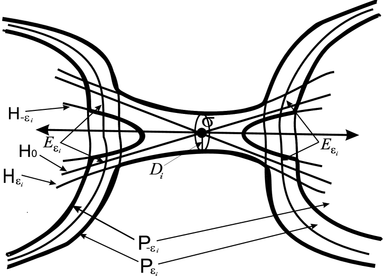
Figure 5: Illustration to step 1

For $t\in[-\varepsilon_{i},\varepsilon_{i}]$ set $Q_{t}=P_{t}\cup H_{t}$. By the construction the set $Q_{t},\leavevmode\nobreak\ t\neq 0$ is $f$-compressed. Moreover, $Q_{-\varepsilon_{i}}$ after smoothing is a handle neighborhood of genus $g_{i-1}$ of the attractor $A_{i-1}$ and $Q_{\varepsilon_{i}}$ after smoothing is strongly tight neighborhood of the attractor $A_{i}$. By assumption of induction and lemma 1 there is a dynamically ordered energy function $\varphi_{{}_{{Q}_{-\varepsilon_{i}}}}$ on ${Q}_{-\varepsilon_{i}}$, which is a constant on $\partial{Q}_{-\varepsilon_{i}}$. As $\varphi_{{}_{{Q}_{-\varepsilon_{i}}}}(A_{i-1})\leq i-1$ then, due to proposition 3, we can suppose that $\varphi_{{}_{{Q}_{-\varepsilon_{i}}}}({Q}_{-\varepsilon_{i}})=i-{\varepsilon_{i}}$.

Define function $\varphi_{{}_{{Q_{\varepsilon_{i}}}}}:Q_{\varepsilon_{i}}\to\mathbb{R}$ on the set $Q_{\varepsilon_{i}}$ by formula:
$\varphi_{{}_{{Q_{\varepsilon_{i}}}}}(x)=\cases{\varphi_{{}_{{Q}_{-\varepsilon_{i}}}}(x),\leavevmode\nobreak\ x\in{Q}_{-\varepsilon_{i}};\cr i+t,\leavevmode\nobreak\ x\in Q_{t}.\cr}$ Let us check that $\varphi_{{}_{{Q_{\varepsilon_{i}}}}}$ is a dynamically ordered energy function $f$, then the existence of required function $\varphi_{{}_{M_{i}}}:M_{i}\to\mathbb{R}$ will follow from lemma 1.

Represent the set ${Q}_{\varepsilon_{i}}$ as a union of subsets with pairwise disjoint interiors: ${Q}_{\varepsilon_{i}}=A\cup B\cup C$, where $A={Q}_{-\varepsilon_{i}}$, $B=P_{\varepsilon_{i}}\setminus{Q}_{-\varepsilon_{i}}$ and $C={Q}_{\varepsilon_{i}}\setminus(P_{\varepsilon_{i}}\cup{Q}_{-\varepsilon_{i}})$. By the construction $\varphi_{{}_{{Q_{\varepsilon_{i}}}}}|_{A}$ a dynamically ordered energy function for $f$, $\varphi_{{}_{{Q_{\varepsilon_{i}}}}}(\partial{A})=i-\varepsilon_{i}$, the function $\varphi_{{}_{{Q_{\varepsilon_{i}}}}}|_{B}$ has no critical points and function $\varphi_{{}_{{Q_{\varepsilon_{i}}}}}|_{C}$ coincides with function $\varphi_{{}_{\mathcal{O}_{i}}}|_{C}$. Let us check decreasing property of $\varphi_{{}_{{Q_{\varepsilon_{i}}}}}$ along trajectories of $f$.

If $x\in A$ then $f(x)\in A$ and $\varphi_{{}_{{Q_{\varepsilon_{i}}}}}(f(x))<\varphi_{{}_{{Q_{\varepsilon_{i}}}}}(x)$, as $\varphi_{{}_{{Q_{\varepsilon_{i}}}}}|_{A}$ is a Lyapunov function. If $x\in B$ then, due to condition (1) of choice of $\varepsilon_{i}$, $f(x)\in A$ and, hence, $\varphi_{{}_{{Q_{\varepsilon_{i}}}}}(x)>i-\varepsilon_{i}$, $\varphi_{{}_{{Q_{\varepsilon_{i}}}}}(f(x))<i-\varepsilon_{i}$, therefor $\varphi_{{}_{{Q_{\varepsilon_{i}}}}}(f(x))<\varphi_{{}_{{Q_{\varepsilon_{i}}}}}(x)$. If $x\in C$ then, due to condition (3) of choice of $\varepsilon_{i}$, either $f(x)\in A$ and decreasing is proved as for $x\in B$, or $f(x)\in C$ and decreasing follows from the fact that $\varphi_{{}_{{Q_{\varepsilon_{i}}}}}|_{C}$ is a Lyapunov function.

Step 2. In this step we delive a construction similar to step 1 for diffeomorphism $f^{-1}$. For this aim we recall that dynamical numbering of the orbits $\mathcal{O}_{1},\dots,\mathcal{O}_{k_{f}}$ of the diffeomorphism $f$ induces dynamical numbering of the orbits $\tilde{\mathcal{O}}_{1},\dots,\tilde{\mathcal{O}}_{k_{f}}$ of the diffeomorphism $f^{-1}$ following way: $\tilde{\mathcal{O}}_{i}=\mathcal{O}_{k_{f}-i}$. Denote by $\tilde{A}_{i}$ the attractors of the diffeomorphism $f^{-1}$, by $\tilde{M}_{i}$ thir neighborhood and by $\tilde{g}_{i}$ a number, defined by formula $\tilde{g}_{i}=\tilde{c}_{i}+\tilde{r}_{i}-\tilde{s}_{i}$, wher $\tilde{c}_{i}$ the number of the connected components of the attractor $\tilde{A}_{i}$, $\tilde{r}_{i}$ the number of the saddle pointd and $\tilde{s}_{i}$ the number of the sink points of the diffeomorphism $f^{-1}$, belonging to $\tilde{A}_{i}$.

Set $\tilde{k}_{1}=k_{f}-k_{1}$ and consider the attrator $\tilde{A}_{\tilde{k}_{1}}$ for the diffeomorphism $f^{-1}$ (which, recall, is a repeller for the diffeomorphism $f$). Similar to step 1 we construct a a dynamically ordered energy function $\tilde{\varphi}_{{\tilde{M}_{\tilde{k}_{1}}}}$ for $f^{-1}$ on the neighborhood ${\tilde{M}_{\tilde{k}_{1}}}$ with level set $\tilde{S}_{\tilde{k}_{1}}=\partial{\tilde{M}_{\tilde{k}_{1}}}$.

Step 3. In this step we show that set $P_{k_{1}}=M\setminus int\leavevmode\nobreak\ \tilde{M}_{\tilde{k}_{1}}$ is a handle neighborhood of genus $g_{k_{1}}$ of the attractor $A_{k_{1}}$, this implies the existence of the required function $\varphi$. Indeed, by lemma 1, the existence of a dynamically ordered energy function $\varphi_{{}_{M_{k_{1}}}}$ on the neighborhood $M_{k_{1}}$ of the attractor $A_{k_{1}}$ implies the existence of a dynamically ordered energy function for $\varphi_{{}_{P_{k_{1}}}}$ on $P_{k_{1}}$ with level set $\partial P_{k_{1}}$. According to proposition 3 the function $\varphi_{{}_{P_{k_{1}}}}$ we can construct such that $\varphi_{{}_{P_{k_{1}}}}(\tilde{S}_{\tilde{k}_{1}})=k_{f}+1-\tilde{\varphi}_{{\tilde{M}_{\tilde{k}_{1}}}}(\tilde{S}_{\tilde{k}_{1}})$. As $\partial P_{k_{1}}=\tilde{S}_{\tilde{k}_{1}}$ then required function $\varphi$ is defined by formula $\varphi(x)=\cases{\varphi_{{}_{P_{k_{1}}}}(x),\leavevmode\nobreak\ x\in P_{k_{1}};\cr k_{f}+1-\tilde{\varphi}_{{\tilde{M}_{\tilde{k}_{1}}}}(x),\leavevmode\nobreak\ x\in{\tilde{M}_{\tilde{k}_{1}}}.\cr}$

Thus, let us prove that the set $P_{k_{1}}=M\setminus int\leavevmode\nobreak\ \tilde{M}_{\tilde{k}_{1}}$ is a handle neighborhood of genus $g_{k_{1}}$ of the attractor $A_{k_{1}}$. Set $\tilde{N}_{\tilde{k}_{1}}=W^{s}_{\tilde{A}_{\tilde{k}_{1}}\cap\Omega_{f^{-1}}}$ and $\tilde{V}_{\tilde{k}_{1}}=\tilde{N}_{\tilde{k}_{1}}\setminus\tilde{A}_{\tilde{k}_{1}}$. Notice that the open sets $V_{k_{1}}$ and $\tilde{V}_{\tilde{k}_{1}}$ are coincide, as both are obtained from $M$ by removing of $A_{k_{1}}$ and $\tilde{A}_{\tilde{k}_{1}}$. It follows from proof of proposition 2 that each of next sets $A_{k_{1}},\leavevmode\nobreak\ \tilde{A}_{\tilde{k}_{1}},M_{k_{1}},\leavevmode\nobreak\ \tilde{M}_{\tilde{k}_{1}},\leavevmode\nobreak\ N_{k_{1}},\leavevmode\nobreak\ \tilde{N}_{\tilde{k}_{1}},\leavevmode\nobreak\ V_{k_{1}},\leavevmode\nobreak\ \tilde{V}_{\tilde{k}_{1}}$ is connected. Then $g_{k_{1}}=1+|\Omega_{1}|-|\Omega_{0}|$ and $\tilde{g}_{\tilde{k}_{1}}=1+|\Omega_{2}|-|\Omega_{3}|$. From statement 3 we get $g_{k_{1}}=\tilde{g}_{\tilde{k}_{1}}$. Thus the handle neighborhoods $M_{k_{1}}$ and $\tilde{M}_{\tilde{k}_{1}}$ have the same genera and their boundaries $S_{k_{1}}$ and $\tilde{S}_{\tilde{k}_{1}}$ belong to the set $V_{k_{1}}$, which is diffeomorphic to $S_{k_{1}}\times\mathbb{R}$.

Choose $n\in\mathbb{N}$ such that $f^{n}(M_{k_{1}})\subset int\leavevmode\nobreak\ P_{k_{1}}$. Then, according to ring hypothesis and corollary 1, manifold $K=P_{k_{1}}\setminus int\leavevmode\nobreak\ f^{n}(M_{k_{1}})$ is diffeomorphic to $S_{k_{1}}\times[0,1]$. By the construction $f^{n}(M_{k_{1}})$ is a handle neighborhood of genus $g_{k_{1}}$ of the attractor $A_{k_{1}}$ and $P_{k_{1}}=f^{n}(M_{k_{1}})\cup K$. This implies that $P_{k_{1}}$ also is handle neighborhood of genus $g_{k_{1}}$ of the attractor $A_{k_{1}}$.

6 Dynamically ordered energy function for diffeomorphisms on 3-sphere

In this section $f:\mathbb{S}^{3}\to\mathbb{S}^{3}$ is a Morse-Smale diffeomorphism without heteroclinic curve.

Proof of theorem 3

Let us prove that diffeomorphism $f$ possesses a dynamically ordered energy function if and only if all its one-dimensional attractors and repellers are tightly embedded.

Proof: The necessity of conditions of the theorem follows from 1, let us proof the sufficiency.

Let $i=k_{0}+1,\dots,k_{1}$. Then $A_{i}$ is one-dimensional attractor, consisting of $c_{i}$ connected components, containing $r_{i}$ saddles, $s_{i}$ sinks and for which a number $g_{i}$ can be calculated by formula $g_{i}=c_{i}+r_{i}-s_{i}$. Firstly prove that $g_{i}=0$ for each $i=k_{0}+1,\dots,k_{1}$.

We start from $g_{k_{1}}$. According to proposition 2, the attractor $A_{k_{1}}$ is connected that is $m_{k_{1}}=1$ and, hence, $g_{k_{1}}=1+|\Omega_{1}|-|\Omega_{0}|$. Due to statement 3, we have $g_{k_{1}}=\tilde{g}_{k_{1}}$, where $\tilde{g}_{k_{1}}=1+|\Omega_{2}|-|\Omega_{3}|$. According to statement 7, $2+|\Omega_{1}\cup\Omega_{2}|-|\Omega_{0}\cup\Omega_{3}|=0$ for any Morse-Smale diffeomorphism without heteroclinic curves on $\mathbb{S}^{3}$. Thus $g_{k_{1}}+\tilde{g}_{k_{1}}=0$ and, hence, $g_{k_{1}}=\tilde{g}_{k_{1}}=0$. Further let us show that $g_{i}\leq g_{i+1}$ for each $i=k_{0},\dots,k_{1}-1$.

Indeed, $g_{i+1}-g_{i}=(c_{i+1}-c_{i})+(r_{i+1}-r_{i})-(s_{i+1}-s_{i})$. At the same time $(c_{i}-c_{i+1})\leq(r_{i+1}-r_{i})$, $s_{i+1}=s_{i}$ and, hence, $g_{i+1}\geq g_{i}$.

Thus, $g_{i}=0$ for each $i=k_{0}+1,\dots,k_{1}$. Then $K_{i}=M_{i}\setminus int\leavevmode\nobreak\ f(M_{i})$ is a union of 3-dimensional annulus $S^{2}\times[0,1]$. As $M_{i}\setminus A_{i}=\bigcup\limits_{k\geq 0}f^{k}(M_{i})$ then $M_{i}\setminus A_{i}$ is diffeomorphic to $\partial M_{i}\times(0,1]$. Thus, the attractor $A_{i}$ is strongly tight embedded. Similar fact has place for repellers. The, according to theorem 2, $f$ possesses a dynamically ordered energy function. $\diamond$

References

- [1] C. Bonatti, V. Grines, O.V. Pochinka, Classification of the Morse-Smale diffeomorphisms with the finite set of heteroclinic orbits on -manifolds. Trudy math. inst. im. V. A. Steklova, v. 250 (2005), 5-53.
- [2] C. Bonatti, V. Grines, V. Medvedev, E. Pecou, Three-manifolds admitting Morse-Smale diffeomorphisms without heteroclinic curves, Topology and its Applications. 117 (2002), 335 344.
- [3] V. Grines, F. Laudenbach, O. Pochinka, An energy function for gradient-like diffeomorphisms on 3-manifolds. (Russian) Dokl. Akad. Nauk 422 (2008), no. 3, 299–301.
- [4] V. Grines, F. Laudenbach, O. Pochinka, Self-indexing energy function for Morse-Smale diffeomorphisms on 3-manifolds, Moscow Math. Journal (2009) 4, 801-821.
- [5] V. Grines, E. Zhuzhoma, V. Medvedev, New relation for Morse-Smale systems with trivially embedded one-dimensional separatrices, Sbornic Math. (2003) 194, 979-1007.
- [6] M.W. Hirsch, Differential Topology, GTM, Springer, 1976.
- [7] J. Milnor, Morse theory, Princeton University Press, 1963.
- [8] J. Palis, On Morse-Smale dynamical systems, Topology (1969) 8, 385-404.
- [9] D. Pixton, Wild unstable manifolds, Topology (1977) 16, 167-172.
- [10] C. Robinson, Dynamical Systems: stability, symbolic dynamics, and chaos, Studies in Adv. Math., Sec. edition, CRC Press. 1999. 506 p.
- [11] S. Smale, Differentiable dynamical systems, Bull. Amer. Math. Soc. (1967) 73, 747-817.
- [12] S. Smale, On gradient dynamical systems, Annals of Math. (1961) 74, 199-206.
- [13] F. Waldhausen, On irreducible 3-manifolds which are sufficiently large, Annals of Math. (1968) 87, 56-88.