Multi-Edge type Unequal Error Protection LDPC Codes

Abstract

Irregular low-density parity check (LDPC) codes are particularly well-suited for transmission schemes that require unequal error protection (UEP) of the transmitted data due to the different connection degrees of its variable nodes. However, this UEP capability is strongly dependent on the connection profile among the protection classes. This paper applies a multi-edge type analysis of LDPC codes for optimizing such connection profile according to the performance requirements of each protection class. This allows the construction of UEP-LDPC codes where the difference between the performance of the protection classes can be adjusted and with an UEP capability that does not vanish as the number of decoding iterations grows.

I Introduction

In communication systems where source bits with different sensitivities to errors are being transmitted, it is often wasteful or even infeasible to provide uniform protection for the whole data stream. In this scenario, the common strategy is the use of schemes with unequal error protection (UEP) capabilities. There are mainly three strategies to achieve UEP on transmission systems: bit loading, multilevel coded modulation, and channel coding [1]. In this paper, we will focus on the latter, more specifically on low-density parity-check (LDPC) codes that provide inherent unequal error protection within a codeword.

Irregular LDPC codes [2] can inherently provide unequal error protection due to the different connection degrees of the coded bits. The connection degrees of the variable and check nodes of such codes are defined by the polynomials $\lambda(x)=\sum_{i=2}^{d_{v_{max}}}\lambda_{i}x^{i-1}$ and $\rho(x)=\sum_{i=2}^{d_{c_{max}}}\rho_{i}x^{i-1}$, where $d_{v_{max}}$ and $d_{c_{max}}$ are the maximum variable and check node degrees of the code. From now on, we will refer to irregular LDPC codes where the variable nodes are divided into disjoint sets called protection classes as unequal error protection LDPC codes (UEP-LDPC).

A flexible optimization of the irregularity profile of irregular LDPC codes based on a hierarchical optimization of the variable node degree distribution was proposed in [3], where the authors interpret the UEP properties of an LDPC code as different local convergence speeds, i.e., the most protected bits are assigned to the bits in the codeword which converge to their right value in the smallest number of iterations. This assumption is made in order to cope with the observation that the UEP gradation vanishes as the number of iterations grow, a fact also observed in [4]. In [5], the authors observed that this vanishing UEP gradation of an iteratively decoded LDPC code is dependent on the algorithm used to construct the parity check matrix, and suggested that the connectivity between the classes is the key factor to be observed if the UEP capabilities should be held as the number of iterations grows.
Herein, we propose an optimization algorithm for the connectivity profile between the different protection classes of LDPC codes in order to not only keep the UEP capability of a code for a moderate to large number of decoding iterations, but also to adjust the performance of the protection classes as required for different applications. This is achieved by means of a multi-edge type (MET) analysis [6, 7] of the LDPC codes. The multi-edge analysis enables us to distinguish between the messages exchanged during the iterative decoding among the different protection classes within one codeword. Thus, we can control the amount of information that the most protected classes receive from the less protected ones and vice versa. If the most protected classes receive a lot of information from the less protected ones, its performance will be decreased while the one of the less protected classes will be enhanced. Our main goal is to show how this exchange of performance among the protection classes can be controlled and optimized.
This paper is organized as follows. In Section II, we describe the multi-edge type analysis of UEP-LDPC codes. Section III discusses the asymptotic analysis of multi-edge type UEP-LDPC codes and the optimization algorithm used to optimize the connection profile between the protection classes. In Section IV, we show the results of the developed optimization method for a chosen example. Finally, some concluding remarks are drawn in Section V.

II Multi-Edge type Unequal Error Protection LDPC Codes

II-A Multi-edge LDPC codes

Multi-edge type LDPC codes [6] are a generalization of irregular and regular LDPC codes. Diverting from standard LDPC ensembles where the graph connectivity is constrained only by the node degrees, in the multi-edge setting, several edge classes can be defined and every node is characterized by the number of connections to edges of each class. Within this framework, the code ensemble can be specified through two multinomials associated to variable and check nodes. The two multinomials are defined by [7]

$$L(\textbf{r},\textbf{x})=\sum L_{\textbf{b},\textbf{d}}\textbf{r}^{\textbf{b}}\textbf{x}^{\textbf{d}},$$ (1)

$$R(\textbf{x})=\sum R_{\textbf{d}}\textbf{x}^{\textbf{d}},$$ (2)

where b, d, r, and x are vectors which are explained as follows. First, let $m_{e}$ denote the number of edge types used to represent the graph ensemble and $m_{r}$ the number of different received distributions. The number $m_{r}$ represents the fact that the different bits can go through different channels and thus, have different received distributions. Each node in the ensemble graph has associated to it a vector $\textbf{x}=(x_{1},...,x_{m_{e}})$ that indicates the different types of edges connected to it, and a vector $\textbf{d}=(d_{1},...,d_{m_{e}})$ referred to as edge degree vector which denotes the number of connections of a node to edges of type $i$, where $i\in(1,\ldots,m_{e})$.

For the variable nodes, there is additionally the vector $\textbf{r}=(r_{1},...,r_{m_{r}})$ which represents the different received distributions, and the vector $\textbf{b}=(b_{0},...,b_{m_{r}})$ that indicates the number of connections to the different received distributions ($b_{0}$ is used to indicate the puncturing of a variable node). In the sequel, we assume that b has exactly one entry set to 1 and the rest set to zero. This simply indicates that each variable node has access to only one channel observation at a time. We use $\textbf{x}^{\textbf{d}}$ to denote $\prod_{i=1}^{m_{e}}x_{i}^{d_{i}}$ and $\textbf{r}^{\textbf{b}}$ to denote $\prod_{i=0}^{m_{r}}r_{i}^{b_{i}}$. Finally, the coefficients $L_{\textbf{b},\textbf{d}}$ and $R_{\textbf{d}}$ are non-negative reals that represent the fraction of variable nodes of type (b,d) and check nodes of type (d) within a codeword, respectively. Furthermore, we have the additional notations defined in [7]

$$L_{r_{i}}(\textbf{r},\textbf{x})=\frac{\mathrm{d}L(\textbf{r},\textbf{x})}{\mathrm{d}r_{i}},$$ (3)

$$L_{x_{i}}(\textbf{r},\textbf{x})=\frac{\mathrm{d}L(\textbf{r},\textbf{x})}{\mathrm{d}x_{i}},$$ (4)

$$R_{x_{i}}(\textbf{x})=\frac{\mathrm{d}R(\textbf{x})}{\mathrm{d}x_{i}}.$$ (5)

Note that in a valid multi-edge ensemble, the number of connections of each edge type should be the same at both variable and check nodes sides. This gives rise to the socket count equality constraint which can be written as

$$L_{x_{i}}(\textbf{1},\textbf{1})=R_{x_{i}}(\textbf{1}),~{}~{}~{}~{}i=1,...,m_{e},$$ (6)

where 1 denotes a vector with all entries equal to 1, with length being clear from the context.

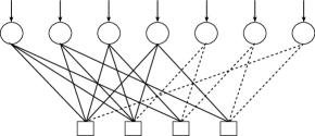
Figure 1: Multi-edge graph with two different edge types and one received distribution.

Unequal error protection LDPC codes can be included in a multi-edge framework in a straightforward way. This can be done by distinguishing between the edges connected to different protection classes within a codeword. According to this strategy, the edges connected to variable nodes within a protection class are all of the same type. For example, in Fig. 1 the first 4 variable nodes can be seen as one protection class since they are connected only to type 1 edges (depicted by solid lines), and the last 3 variable nodes compound another protection class, since they are only connected to type 2 edges (depicted by the dashed lines). It is worth noting that opposed to the variable nodes, the check nodes admit connections with edges of different types simultaneously as can be inferred from Fig.1. In the following, we will divide the variable nodes into $m_{e}$ protection classes $(C_{1},C_{2},\ldots,C_{m_{e}})$ with degrading levels of protection.

II-B Edge perspective notation

The connection between the protection classes occurs through the check nodes since they can have different types of edges attached to them. Consider irregular LDPC codes with node perspective variable and check node multi-edge multinomials $L(\textbf{r},\textbf{x})=\sum L_{\textbf{b},\textbf{d}}\textbf{r}^{\textbf{b}}\textbf{x}^{\textbf{d}}$ and $R(\textbf{x})=\sum R_{\textbf{d}}\textbf{x}^{\textbf{d}}$, respectively.

In order to implement the optimization algorithm, it will be more convenient to work with the edge, instead of the node perspective. We now define edge perspective multi-edge multinomials. Let $\rho_{\textbf{d}}^{(j)}$ denote the fraction of type $j$ ($j=1,\ldots,m_{e}$) edges connected to check nodes of type d. The fraction $\rho_{\textbf{d}}^{(j)}$ is calculated with respect to the total number of edges of type $j$ and is thus given by

$$\rho_{\textbf{d}}^{(j)}=\frac{d_{j}R_{\textbf{d}}}{R_{x_{j}}(\textbf{1})}.$$ (7)

Similarly, let $\lambda_{i}^{(j)}$ denote the fraction (computed with respect to the total number of type $j$ edges) of type $j$ edges connected to variable nodes of degree $i$. This gives us the following edge perspective multinomial

$$\lambda^{(j)}(x)=\sum_{i}\lambda_{i}^{(j)}x^{i-1},$$ (8)

where $\lambda_{i}^{(j)}$ represents the fraction of class $j$ edges connected to variable nodes with degree $i$. In the next section, we will use Eqs. (7) and (8) in the derivation of the optimization algorithm for the connection profile among the protection classes of an UEP-LDPC code.

III Check node profile optimization

III-A Asymptotic Analysis

Our main objective is, given the overall variable and check node degree distributions of an UEP-LDPC code, to optimize the connection profiles between the different protection classes in order to control the amount of protection of each class while preserving the UEP capability of the code after a moderate to high number of decoding iterations. In order to simplify the optimization algorithm, we suppose that the LDPC code to be optimized is check-regular, i.e., all the check nodes have the same degree.

Despite of having the same degree, each check node may have a different number of edges belonging to each one of the $m_{e}$ classes. Consider for example a check node with an associated edge degree vector $\textbf{d}=(d_{1},d_{2},\ldots,d_{m_{e}})$, where $d_{i}$ is the number of connections to the protection class $i$ and $\sum_{i=1}^{m_{e}}d_{i}=d_{c_{max}}$. If we then consider a code with $m_{e}=3$ protection classes, each check node may be connected to $d_{1}$ edges of class 1, $d_{2}$ edges of class 2, and $d_{3}$ edges of class 3. This posed, one can compute the evolution of the iterative decoding by means of density evolution.

We assume here standard belief propagation decoding of LDPC codes where the messages exchanged between the variable and check nodes are log-likelihood ratios having a symmetric Gaussian distribution (variance equals twice the mean). Before dealing with the subtle case of irregular multi-edge type LDPC codes, let’s make for now two simplifying assumptions: 1) All variable nodes have the same degree $d_{v}$. 2) All check nodes have the same edge degree vector d.

Under these assumptions, we can generalize the results obtained in [8] for regular LDPC codes and compute the mutual information between the output message of a class $C_{j}$, degree-$d_{v}$ variable node and the observed channel value at iteration $l$, which is given by

$$I_{v,l}^{C_{j}}=J\left(\sqrt{4/\sigma^{2}+(d_{v}-1)[J^{-1}(I_{c,{l-1}}^{C_{j}})]^{2}}\right),$$ (9)

where $\sigma^{2}$ is the channel noise variance, $I_{c,l-1}^{C_{j}}$ is the mutual information received from the neighboring check nodes at iteration $l-1$ and the $J(.)$ function is defined as in [9]

$$J(\sigma)=1-\int_{-\infty}^{\infty}\frac{e^{\frac{(\xi-\sigma^{2}/2)^{2}}{2\sigma^{2}}}}{\sqrt{2\pi}\sigma}\cdot\log_{2}[1+e^{-\xi}]d\xi~{}.$$ (10)

Similarly, the mutual information sent to the variable nodes of class $C_{j}$ from a check node with an associated vector d can be expressed as

$$I_{c,l}^{C_{j}}=1$$

$$-J\left(\sqrt{(d_{j}-1)(J^{-1}(1-I_{v,l}^{C_{j}}))^{2}+\sum_{i\neq j}d_{i}(J^{-1}(I_{v,l}^{C_{i}}))^{2}}\right).$$ (11)

Let’s now deal with the more general case of irregular codes. For irregular codes, the incoming densities to a node are not necessarily equal due to varying degrees. Therefore, the overall mutual information at the output of the variable and check nodes is averaged over the different degrees. Also note that, in the irregular case, for optimizing the connection profile between the protection classes, we need to consider the case where check nodes with different edge degree vector d are allowed. This posed, the mutual information between the received channel values and the messages sent from the check to variable nodes and from variable to check nodes at iteration $l$ within the protection class $C_{j}$, computed by means of density evolution using the Gaussian approximation [10], are given by

$$I_{v,l}^{C_{j}}=\sum_{i=2}^{d_{v_{max}}}\lambda_{i}^{(j)}J\left(\sqrt{4/\sigma^{2}+(i-1)[J^{-1}(I_{c,{l-1}}^{C_{j}})]^{2}}\right),$$ (12)

$$I_{c,l}^{C_{j}}=1-\sum_{s=1}^{d_{c_{max}}}\sum_{\textbf{d}:d_{j}=s}\rho_{\textbf{d}}^{(j)}$$

$$\cdot J\left(\sqrt{(d_{j}-1)J^{-1}(1-I_{v,l}^{C_{j}})^{2}+\sum_{i\neq j}d_{i}J^{-1}(1-I_{v,l}^{C_{i}})^{2}}\right).$$ (13)

Combining Eqs. (12) and (13), one can summarize the density evolution as a function of the mutual information of the previous iteration, the mutual information contribution from the other classes, noise variance, and degree distributions

$$I_{l}^{C_{j}}=F(\lambda^{(j)}(x),\rho_{\textbf{d}}^{(j)},\sigma^{2},I_{l-1}^{C_{j}},I_{l-1}^{C_{i}}),$$ (14)

where $i\in(1,\ldots,m_{e})$ and $i\neq j$. By means of Eq. (14), we can predict the convergence behavior of the decoding and than optimize the degree distribution $\rho_{\textbf{d}}^{(j)}$ under the constraint that the mutual information shall be increasing as the number of iterations grow, i.e.,

$$F(\lambda^{(j)}(x),\rho_{\textbf{d}}^{(j)},\sigma^{2},I^{C_{j}},I^{C_{i}})>I^{C_{j}}.$$ (15)

At this point, it is worth noting that, as pointed out in [4] and [5], the UEP capabilities of a code depend on the amount of connection among the protection classes, i.e., if the most protected class is well connected to the least protected one, the performance of the former will decrease while the performance of the latter will be improved. For example, suppose a code with 2 protection classes and $d_{c_{max}}=4$. The possible values for $\textbf{d}=(d_{1},d_{2})$ are (0,4), (1,3), (2,2), (3,1), and (4,0). On the one hand, if a code has a majority of check nodes with $\textbf{d}=(4,0)$, the first protection class will be very isolated from class 2 which will lead to an enhanced performance difference between the two classes. On the other hand, if a large amount of the check nodes are of type $\textbf{d}=(2,2)$, one can expect the protection classes to be very connected, which favors the overall performance but mitigates the UEP capability of a code at a moderate to large number of decoding iterations. This indicates that for controlling the UEP capability of an LDPC code and to prevent this characteristic from vanishing as the number of decoding iterations grows, one has to control the amount of check nodes of each type, i.e., optimize $\rho_{\textbf{d}}^{(j)}$.

III-B Optimization Algorithm

The algorithm described here aims at optimizing the connection profile between the various protection classes present on a UEP-LDPC code, i.e., $\rho_{\textbf{d}}^{(j)}$. Initially, the algorithm computes the variable node degree distribution of each class $\lambda^{(j)}(x)$ based on $\lambda(x)$, $d_{c_{max}}$, and the number of edges on each class. The algorithm then proceeds sequentially optimizing the connection profile to the check nodes of one class at a time, proceeding from the less protected class to the most protected one. This scheduling is done in order to control the amount of messages coming up from the less protected classes that are forwarded to the more protected ones.

Since we are using linear programming (LP) with only a single objective function, we chose it to be the minimization of the average check node degree within the class being optimized, i.e., it minimizes the average number of edges of such a class connected to the check nodes. This minimization aims at diminishing the amount of unreliable messages (i.e., the ones coming up from the less protected variable nodes) that flows through a check node. In addition to it, we control the proportion of check nodes of type $\mathbf{d}$ introducing the parameter $max{\rho_{\textbf{d}}^{(j)}}$ which is an upper bound on $\sum_{\textbf{d}:d_{j}=s}\rho_{\textbf{d}}^{(j)}$, i.e., it limits the proportion of check nodes of type $\textbf{d}:d_{j}=s$ for $s=0,\ldots,d_{c_{max}}$, thus regulating the degree of connection among the protection classes. For example, setting $max{\rho_{\textbf{d}}^{(j)}}=0.35$ means that the maximum fraction of check nodes with edge degree vector d (for any d) will be 0.35.

The optimization is then performed for each class $C_{j}$ by minimizing its average check node degree for a decreasing $d_{min}^{(j)}$ from $d_{c_{max}}$ to 1, where $d_{min}^{(j)}$ is the minimum number of edges of class $j$ connected to a check node. At this point, one can argue that since our goal is to minimize the average connection degree within a protection class, we should thus set $d_{min}^{(j)}=1$. The problem with this strategy is that it would shorten the degree of freedom for the optimization of the next class, e.g., suppose the optimization of a two-class code with $d_{min}^{(2)}=3$ and $d_{c_{max}}=5$. Once we proceed to the optimization of class two, the coefficients $\rho_{(2,3)}^{(2)}$, $\rho_{(1,4)}^{(2)}$ , and $\rho_{(0,5)}^{(2)}$ are determined and consequently fixed for the next optimization step, i.e., the optimization of class 1, we will have as variables only the coefficients $\rho_{(3,2)}^{(1)}$, $\rho_{(4,1)}^{(1)}$, and $\rho_{(5,0)}^{(1)}$. Note that in this case, if we had set $d_{min}^{(2)}=1$, there will be no degree of freedom for optimizing class 1 since the only non-optimized $\mathbf{d}$ would be $\mathbf{d}=(5,0)$ which would be determined by $\sum_{s=d_{min}^{(j)}}^{d_{c_{max}}}\sum_{\textbf{d}:d_{j}=s}\rho_{\textbf{d}}^{(j)}=1$, i.e., the sum of all fraction of edges must be equal to one.

The iterative procedure is successful, when a solution $\rho_{\textbf{d}}^{(j)}$ is found which converges for the given $\sigma^{2}$ and $d_{min}^{(j)}>0$. We assume that the optimizations for classes $\{C_{j^{\prime}},j^{\prime}<j\}$ have already been performed and the results of these optimizations are used as constraints in the current optimization process. The optimization algorithm can be written, for given $\lambda(x)$, $\sigma^{2}$, $m_{e}$, $d_{c_{max}}$, and $max\rho_{\textbf{d}}^{(j)}$ for $j=1,\ldots,m_{e}$ as shown in Fig. 2.

1. Compute $\lambda^{(j)}(x)$ 2. Initialization $d_{min}^{(j)}=d_{c_{max}}$ 3. While optimization failure (a) minimize the average check node degree
$\sum_{s=d_{min}^{(j)}}^{d_{c_{max}}}s\cdot\sum_{\textbf{d}:d_{j}=s}\rho_{\textbf{d}}^{(j)}$ under the
following constraints, $\mathcal{C}_{1}$ :$\sum_{s=d_{min}^{(j)}}^{d_{c_{max}}}\sum_{\textbf{d}:d_{j}=s}\rho_{\textbf{d}}^{(j)}=1$, $\mathcal{C}_{2}$ :$\sum_{\textbf{d}:d_{j}=s}\rho_{\textbf{d}}^{(j)}\in[0,max\rho_{\textbf{d}}^{(j)}]$, $\mathcal{C}_{3}$ :$F(\lambda^{(j)}(x),\rho_{\textbf{d}}^{(j)},\sigma^{2},x,I^{C_{j}},I^{C_{i}})>x$, $\forall x\in[0,1)$ and $i\neq j$, $\mathcal{C}_{4}$ :$\forall j^{\prime}>j$ and $\textbf{d}:d_{j^{\prime}_{min}}\leq d_{j^{\prime}}\leq d_{c_{max}},\\ \rho_{\textbf{d}}^{(j)}$ is fixed. b) $d_{min}^{(j)}=d_{min}^{(j)}-1$ End (While)

Figure 2: Check node profile optimization algorithm.

Note that the optimization can be solved by linear programming since the cost function and the constraints ($\mathcal{C}_{1}$), ($\mathcal{C}_{2}$), and ($\mathcal{C}_{3}$) are linear in the parameters $\rho_{\textbf{d}}^{(j)}$. The constraint ($\mathcal{C}_{4}$) is the previous optimization constraint. Once we have optimized the check node profile, the code can be realized through the construction of a parity check matrix following the desired profile.

IV Simulation Results

In this section, simulation results for multi-edge type UEP-LDPC codes with optimized check node connection profile are presented. We designed UEP-LDPC codes of length $n=4096$ with $m_{e}=3$ protection classes, rate 1/2, and $d_{v_{max}}=30$ following the algorithm of [3]. The proportions of the classes are chosen such that $C_{1}$ contains 20% of the information bits and $C_{2}$ contains 80%. The third protection class $C_{3}$ contains all parity bits. Therefore, we are mainly interested in the performances of classes $C_{1}$ and $C_{2}$. The optimized variable and check node degree distribution for the UEP-LDPC code are given by $\lambda(x)=0.2130x+0.0927x^{2}+0.2511x^{3}+0.2521x^{17}+0.0965x^{18}+0.0946x^{29}$ and $\rho(x)=x^{8}$, respectively.

In order to have a low-complexity systematic encoder, we construct parity check matrices in lower triangular form [11]. This approach also leads to a simplification in our optimization procedure, i.e., given that the parity bits are in the less protected class $C_{3}$ and that they should be organized in a lower triangular form, we start the optimization from the less protected information bits class $C_{2}$, since all the connections between the variable nodes of class $C_{3}$ and the check nodes are completely determined by the lower triangular form construction algorithm. Table I summarizes the classes’ variable degree distributions $\lambda^{(j)}(x)$.

TABLE I: Local variable degree distributions. The coefficients $\lambda_{i}^{(j)}$ represent the fraction of edges connected to variables nodes of degree $i$ within the class $C_{j}$.

$C_{1}$	$C_{2}$	$C_{3}$
$\lambda_{4}^{(1)}=0.00197$	$\lambda_{3}^{(2)}=0.23982$	$\lambda_{2}^{(3)}=0.93901$
$\lambda_{18}^{(1)}=0.57263$	$\lambda_{4}^{(2)}=0.76018$	$\lambda_{3}^{(3)}=0.06099$
$\lambda_{19}^{(1)}=0.21085$
$\lambda_{30}^{(1)}=0.21455$

We applied the optimization algorithm for different values of $max\rho_{\textbf{d}}^{(j)}$ to enable the observation of the varying UEP capabilities of the codes. The resulting distributions are summarized in Table II. All the simulations were done for a total of 50 decoding iterations and the constructed codes were all realized through a modification of progressive edge-growth (PEG) [12] algorithm done in order to ensure that the optimized check node degree is realized.

TABLE II: Optimized check node profile for 3 protection classes. The coefficients $\rho_{s}^{(j)}$ represent $\rho_{\textbf{d}}^{(j)}$ with $\textbf{d}:d_{j}=s$.

	$C_{1}$	$C_{2}$	$C_{3}$
$max\rho_{\textbf{d}}^{(2)}=0.35$	$\rho_{2}^{(1)}=0.08977$	$\rho_{2}^{(2)}=0.35$	$\rho_{1}^{(3)}=0.00024$
	$\rho_{3}^{(1)}=0.19637$	$\rho_{3}^{(2)}=0.35$	$\rho_{2}^{(3)}=0.93877$
	$\rho_{4}^{(1)}=0.34911$	$\rho_{4}^{(2)}=0.30$	$\rho_{3}^{(3)}=0.06099$
	$\rho_{7}^{(1)}=0.36475$
$max\rho_{\textbf{d}}^{(2)}=0.55$	$\rho_{3}^{(1)}=0.25248$	$\rho_{3}^{(2)}=0.45$	$\rho_{1}^{(3)}=0.00024$
	$\rho_{4}^{(1)}=0.54860$	$\rho_{4}^{(2)}=0.55$	$\rho_{2}^{(3)}=0.93877$
	$\rho_{7}^{(1)}=0.19892$		$\rho_{3}^{(3)}=0.06099$
$max\rho_{\textbf{d}}^{(2)}=0.75$	$\rho_{3}^{(1)}=0.14027$	$\rho_{3}^{(2)}=0.25$	$\rho_{1}^{(3)}=0.00024$
	$\rho_{4}^{(1)}=0.74809$	$\rho_{4}^{(2)}=0.75$	$\rho_{2}^{(3)}=0.93877$
	$\rho_{7}^{(1)}=0.11164$		$\rho_{3}^{(3)}=0.06099$

Figure 3 shows that the difference in the performances of the protection classes is reduced as we increase the value of $max\rho_{\textbf{d}}^{(2)}$. This is an expected effect, since the greater $max\rho_{\textbf{d}}^{(2)}$, the greater is the amount of information that $C_{2}$ exchanges with $C_{1}$. Obviously, this is expected to enhance the performance of $C_{2}$ while lowering the one of $C_{1}$. Furthermore, despite the already large number of decoding iterations (50 iterations), the UEP capability is preserved, something regarded as infeasible in [3] and not observed in [5] for codes realized by means of PEG.

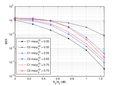
Figure 3: Classes bit error rate of the optimized multi-edge unequal error protection LDPC codes for different values of $max\rho_{\textbf{d}}^{(2)}$.

V Concluding remarks

In this paper, we introduced a multi-edge type analysis of unequal error protection LDPC codes. By means of such an analysis, we derived an optimization algorithm that aims at optimizing the connection profile between the protection classes within a codeword. This optimization allowed us not only to control the differences in the performances of the protection classes by means of a single parameter, but also to prevent the UEP capability of an LDPC code to vanish after a moderate to large number of decoding iterations.

References

- [1] W. Henkel, K. Hassan, N. von Deetzen, S. Sandberg, L. Sassatelli, and D. Declercq, “UEP concepts in modulation and coding,” Hindawi, Advances in Multimedia, Vol. 2010, Article ID 416797, 14 pages, 2010. doi:10.1155/2010/416797.
- [2] T. Richardson, M. Shokrollahi, and R. Urbanke, “Design of capacity-approaching irregular low-density parity-check codes,” IEEE Transactions on Information Theory, vol. 47, no. 2, pp. 619–637, Feb. 2001.
- [3] C. Poulliat, D. Declercq, and I. Fijalkow, “Enhancement of unequal error protection properties of LDPC codes,” EURASIP Journal on Wireless Communications and Networking, vol. 2007, Article ID 92659, 9 pages, doi:10.115/2007/92659.
- [4] V. Kumar and O. Milenkovic, “On unequal error protection LDPC codes based on Plotkin-type constructions,” IEEE Transactions on Communications, vol. 54, no. 6, pp. 994–1005, 2006.
- [5] N. von Deetzen and S. Sandberg, “On the UEP capabalities of several LDPC construction algorithms,” IEEE Transactions on Communications, vol. 58, no. 11, pp. 3041–3046, November 2010.
- [6] T. Richardson and R. Urbanke, “Multi-Edge Type LDPC Codes,” Tech. Rep., 2004, submitted to IEEE Transaction on Information Theory.
- [7] ——, Modern Coding Theory. Cambridge University Press, 2008.
- [8] A. Ashikhmin, G. Kramer, and S. ten Brink, “Extrinsic information transfer functions: model and erasure channel properties,” IEEE Transactions on Information Theory, vol. 50, no. 11, pp. 2657–2673, Nov. 2004.
- [9] S. ten Brink, “Convergence behavior of iteratively decoded parallel concatenated codes,” IEEE Transactions on Communications, vol. 49, no. 10, pp. 1727–1737, Oct. 2001.
- [10] S. Y. Chung, T. Richardson, and R. Urbanke, “Analysis od sum-product decoding of low-density parity-check codes using a Gaussian approximation,” IEEE Transactions on Information Theory, vol. 47, no. 2, pp. 657–670, Feb. 2001.
- [11] T. Richardson and R. Urbanke, “Efficient encoding of low-density parity-check codes,” IEEE Transactions on Information Theory, vol. 47, no. 2, pp. 638–656, Feb. 2001.
- [12] X.-Y. Hu, E. Eleftheriou, and D. M. Arnold, “Regular and irregular progressive edge-growth tanner graphs,” IEEE Transactions on Information Theory, vol. 51, no. 1, pp. 386–398, January 2005.