BU-HEPP-10-07
CERN-PH-TH/2011-029
Jan., 2011

Magic Spinor Product Methods in Loop Integrals^†

B.F.L. Ward
Department of Physics,
Baylor University, Waco, Texas, USA
and
CERN, Geneva, Switzerland

Abstract

We present an approach to higher point loop integrals using Chinese magic in the virtual loop integration variable. We show, using the five point function in the important $e^{+}e^{-}\rightarrow f\bar{f}+\gamma$ process for ISR as a pedagogical vehicle, that we get an expression for it directly reduced to one scalar 5-point function and 4-, 3-, and 2- point integrals, thereby avoiding the computation of the usual three tensor 5-pt Passarino-Veltman reduction. We argue that this offers potential for greater numerical stability.

• Work partly supported by US DOE grant DE-FG02-09ER41600.

With the advent of the LHC, we enter the era of precision QCD, by which we mean predictions for QCD processes at the total precision tag of $1\%$ or better. This is analogous to the per mille level era of EW corrections at LEP energies. Radiative effects at the level of ${\cal O}(\alpha_{s}^{2})$ have to be controlled on the QCD side and those at the level of ${\cal O}(\alpha L\alpha_{s}),\;{\cal O}(\alpha^{2}L^{2})$ on the QED$\otimes$QCD and QED sides have to be controlled systematically, both from the physical precision standpoint and from the technical precision standpoint, in order to optimize physics discovery at the LHC. In Ref. [1], we have developed a platform for the realization of such corrections ultimately on an event-by-event basis based on exact, amplitude-based resummation of QED and QCD together, wherein residuals for hard photons and hard gluons are simultaneously calculated order-by-order in perturbation theory in powers of $\alpha$ and $\alpha_{s}$. These residuals, which are infrared finite and, for hadron-hadron applications, collinearly finite require then exact evaluation of higher point and (higher) loop Feynman diagrams in an appropriate reduction scheme for any attendant tensor properties as first developed systematically in Ref. [2], for example. Recently, alternative approaches have been developed in Refs. [3, 4] to deal with the growing complexity of the method in Ref. [2] as the number of legs beyond four and/or loops beyond one increases. Here, we focus on higher point one-loop functions.

It has been demonstrated that n-point functions, for $n=1,\cdots,4$, at one-loop, reduced to scalar functions using the method of Ref. [2], are tractable for fast MC event generator implementation for arbitrary masses and kinematics for high energy scattering processes [6, 7, 8, 9, 10, 11, 12, 13, 14, 15, 16, 17, 18, 19, 20, 21, 22]. It has also been demonstrated [23, 24, 25, 26] that, at one-loop, higher point scalar functions can be reduced to sums of four-point scalar functions. In Refs. [24, 27, 28, 29, 30] representations of the scalar four-point function that cover arbitrary masses and the momenta relevant to most high energy collider applications have been given and these are suitable for fast MC implementation. Thus, when one is discussing higher point functions at one-loop, we can consider, at least for most collider physics applications, that the 1, 2, 3 and 4 point functions at one-loop are known in a practical way so that the main issue can be considered to be the representation of the higher point functions in terms of these known functions.

When we consider any higher point function, two of the most important aspects of any reduction procedure for recasting it in terms of the “known”, lower point functions are its numerical stability and its usefulness for Monte Carlo event generator realization, as we have in mind for our residuals $\hat{\tilde{\bar{\beta}}}_{n,m}$ in Refs. [1] for example. Given the simplification that has been shown for the “Chinese magic” polarization scheme [31, 32, 33] for real emission of massless gauge particles in such functions, it is natural to seek further simplification and numerical stability in the virtual emission and re-absorption processes as well by exploiting the same scheme. It is this that we pursue in what follows.

For the reader unfamiliar with the “Chinese magic” polarization scheme for massless gauge bosons, which is historically associated to the preprint in Ref. [31], the key observation is that the gauge invariance of the attendant massless gauge theory allows one to use an attendant set of polarization vectors which, when the chiral forms of the respective spin $\frac{1}{2}$ charged particles’ wave functions are used, eliminate radiation from one entire side of a charged line and, simultaneously, simplify considerably the calculation of the part of the amplitude that remains, almost like “magic, hence the name. This is possible because of a representation of the respective polarization vector for helicity $\lambda_{\gamma}$ and 4-momentum $k_{\gamma}$, $\epsilon_{\lambda_{\gamma}}^{\mu}$, as a matrix element of the Dirac gamma matrix, $\gamma^{\mu}$, between the spinor of helicity $\lambda_{\gamma}$ and four-momentum $k_{\gamma}$, $|k_{\gamma}\lambda_{\gamma}>$, and the massless spinor state $<\rho\lambda_{\gamma}|,\;\rho^{2}=0$, up to a normalization factor, so that the Chisholm identity (see eq.(12) below) reduces the Feynman rule factor $\epsilon_{\lambda_{\gamma}}^{*\mu}\gamma_{\mu}$ at the respective interaction vertex to the simple expression $2[|k_{\gamma}-\lambda_{\gamma}><\rho-\lambda_{\gamma}|+|\rho\lambda_{\gamma}><k_{\gamma}\lambda_{\gamma}|]$, up to the same normalization factor, which causes one side of a line of the real radiation terms to vanish if $\rho$ is set equal to the external 4-momentum entering(leaving) that side of the respective line. The remaining terms are then expressed in terms of simple spinor products which lend themselves to easy evaluation [31, 32, 33]. This gives a ’magically’ shortened expression compared the usual Cartesian representation of the polarization vector with the squared amplitude modulus evaluated using traces over the fermion lines. We illustrate this below here as well.

Specifically, we will use the conventions of Ref. [10, 34] for spinors and polarization vectors, which are derived from the work of  [31, 33]. The 5-pt function which we want to analyze in these conventions as our prototypical example is shown in diagram (c) in Fig. 1.

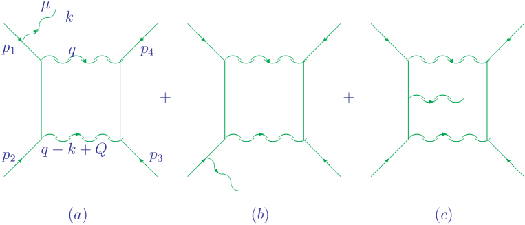
Figure 1: ISR 5-point function contributions with fermion and vector boson masses $m_{f},~{}m_{B},\;f=1,2,\;B=V_{1},V_{2}$ and with four momenta $p_{i},~{}k$ as shown, with $Q\equiv p_{1}+p_{2}$. Radiation is shown from the initial state line with electric charge $Q_{1}e$ where $e$ is the electric charge of the positron – here $p_{1}$ is the incoming fermion 4-momentum, $p_{2}$ is the incoming anti-fermion 4-momentum. When the quantum numbers allow it, the crossed graphs for the internal vector boson exchanges must be added to what we show here.

It has many applications in collider precision physics. When combined with diagrams 1(a) and 1(b) it generates a gauge invariant contribution to the ISR for $e^{+}e^{-}\rightarrow f\bar{f}+\gamma$, $f\neq e$ , for example, and it is a part of such a contribution to $u\bar{u}\rightarrow\mu\bar{\mu}+G$ (in an appropriate color basis), etc. Such applications and their attendant phenomenology will be taken up elsewhere. [36]. Here, we focus on the use of Chinese magic in the loop integral in Fig. 1(c) to illustrate what simplifications are possible.

More precisely, by the standard methods, we need the following Feynman integral representation of Fig. 1(c)

$$\begin{split}{\cal M}^{(1c)}_{\lambda_{1}\lambda_{2}\lambda^{\prime}_{1}\lambda^{\prime}_{2}\lambda_{\gamma}}&=(2\pi)^{4}\delta(p_{1}+p_{2}-p^{\prime}_{1}-p^{\prime}_{2}-k){\cal C}\frac{\int d^{4}q}{(2\pi)^{4}}\frac{\bar{v}_{\lambda_{2}}\gamma^{\beta}(\not\!q+\not\!p_{1}-\not\!k+m_{1})\not\!\epsilon^{*}_{\lambda_{\gamma}}(\not\!q+\not\!p_{1}+m_{1})\gamma^{\alpha}u_{\lambda_{1}}}{((q+p_{1}-k)^{2}-m_{1}^{2}+i\epsilon)((q+p_{1})^{2}-m_{1}^{2}+i\epsilon)}\\ &\quad\frac{\bar{u}^{\prime}_{\lambda^{\prime}_{1}}\gamma_{\alpha}(\not\!q+\not\!p^{\prime}_{1}+m_{2})\gamma_{\beta}v^{\prime}_{\lambda^{\prime}_{2}}}{((q+p_{1}+p_{2}-k)^{2}-M_{V_{2}}^{2}+i\epsilon)((q+p^{\prime}_{1})^{2}-m_{2}^{2}+i\epsilon)(q^{2}-M_{V_{1}}^{2}+i\epsilon)}+\ldots,\end{split}$$ (1)

where we have defined massless limit coupling factor

$${\cal C}={\cal C}(\{\lambda_{i}\},\{\lambda^{\prime}_{j}\})=Q_{1}eG^{2}G^{\prime 2}(v^{\prime}_{1}+a^{\prime}_{1}\lambda_{2})(v_{1}-a_{1}\lambda_{1})(v^{\prime}_{2}+a^{\prime}_{2}\lambda^{\prime}_{2})(v_{2}-a_{2}\lambda^{\prime}_{1})$$ (2)

with the couplings $Q_{1}e,\;G\;\text{and}\;G^{\prime}$ for the $\gamma,\;V_{1}\;\text{and}\;V_{2}$, respectively. In the usual Glashow-Salam-Weinberg-’t Hooft-Veltman [37] notation, v(a) represents vector(axial-vector) coupling. The ellipsis in (1) represent the mass corrections needed to correct the massless limit used for ${\cal C}(\{\lambda_{i}\},\{\lambda^{\prime}_{j}\})$. They are not necessary to illustrate our method and they will be restored elsewhere [36]. To get the loop integral in terms of Chinese magic, we take the following kinematics as shown in Fig. 1:

$$p_{1} = (E,p\hat{z})$$

$$p_{2} = (E,-p\hat{z})$$

$$-p_{4} = (E^{\prime},p^{\prime}(\cos\theta^{\prime}_{1}\hat{z}+\sin\theta^{\prime}_{1}\hat{x}))\equiv p^{\prime}_{1}$$

$$k = (k^{0},k(\cos\theta_{\gamma}\hat{z}+\sin\theta_{\gamma}(\cos\phi_{\gamma}\hat{x}+\sin\phi_{\gamma}\hat{y})))$$

$$-p_{4}-p_{3}+k = p_{1}+p_{2}=(\sqrt{s},\vec{0})$$

$$-p_{3} \equiv p^{\prime}_{2}$$ (3)

with $k^{0}=k$, $\sqrt{s}=2E$. Here, we introduce the alternate notations $p^{\prime}_{1}=-p_{4},\;p^{\prime}_{2}=-p_{3}$ for cosmetic use entirely. We now introduce the two sets of magic polarization vectors associated to the two incoming lines:

$$(\epsilon^{\mu}_{\sigma}(\beta))^{*}={\bar{u}_{\sigma}(k)\gamma^{\mu}u_{\sigma}(\beta)\over\sqrt{2}\;\bar{u}_{-\sigma}(k)u_{\sigma}(\beta)},\quad(\epsilon^{\mu}_{\sigma}(\zeta))^{*}={\bar{u}_{\sigma}(k)\gamma^{\mu}{\color[rgb]{0,0,0}\mathfrak{u}}_{\sigma}(\zeta)\over\sqrt{2}\;\bar{u}_{-\sigma}(k){\color[rgb]{0,0,0}\mathfrak{u}}_{\sigma}(\zeta)},$$ (4)

with $\beta^{2}=0$ and $\zeta$ defined in Ref. [10, 34], so that all phase information is strictly known in our amplitudes: the two choices for $\beta$ are such that its space-like components have the directions of the two incoming beams in the initial state. We take the the basis of the 4-dimensional momentum space as follows:

$$\begin{split}\ell_{1}&=(E,E\hat{z}),\;\ell_{2}=(E,-E\hat{z})\cr\ell_{3}&=E\frac{<\ell_{2}+|\gamma^{\mu}|\ell_{1}+>}{\sqrt{2}<\ell_{2}-|\ell_{1}+>}\cr&=\quad\frac{-E}{\sqrt{2}}(\hat{x}+i\hat{y})\cr\ell_{4}&=E\frac{<\ell_{2}-|\gamma^{\mu}|\ell_{1}->}{\sqrt{2}<\ell_{2}+|\ell_{1}->}\cr&=\quad\frac{E}{\sqrt{2}}(\hat{x}-i\hat{y})\end{split}$$ (5)

where we use the obvious equivalence $|\ell\sigma>=u(\ell)_{\sigma}$ in the notation of Refs. [31, 32, 33, 34]. The important point is that all four of these basis 4-vectors are light-like with $\ell_{i}^{2}=0,\;i=1,\cdots,4$.They therefore can participate in Chinese magic.

To illustrate explicitly this latter point, consider the definite case $\lambda_{1},\lambda_{2},\lambda^{\prime}_{1},\lambda^{\prime}_{2},\lambda_{\gamma}=+,-,+,-,+$, as all other choices for the helicities behave similarly. We write the loop momentum as

$$q=\alpha_{i}\ell_{i}$$ (6)

with summation over repeated indices understood. The coefficients $\alpha_{i}$ are readily determined as

$$\begin{split}\alpha_{1}&=\frac{q\ell_{2}}{2E^{2}}=({\mathfrak{D}}_{3}-{\mathfrak{D}}_{2}-s+2p_{2}k+M_{V_{2}}^{2})/s\cr\alpha_{2}&=\frac{q\ell_{1}}{2E^{2}}=({\mathfrak{D}}_{1}-{\mathfrak{D}}_{0}-M_{V_{1}}^{2})/s\cr\alpha_{3}&=\frac{q\ell_{4}}{E^{2}}=-\frac{q\ell^{*}_{3}}{E^{2}}=-\alpha^{*}_{4}\cr\alpha_{4}&=-\frac{i}{\sqrt{2s}}[c_{j}{\mathfrak{D}}_{j}+c_{5}M_{V_{1}}^{2}+c_{6}(M_{V_{2}}^{2}+2p_{2}k-s)+c_{7}(2kp_{1})]\end{split}$$ (7)

where we define the denominators as

$$\begin{split}{\mathfrak{D}}_{0}&=q^{2}-M_{V_{1}}^{2}+i\epsilon\cr{\mathfrak{D}}_{1}&=(q+p_{1})^{2}-m_{1}^{2}+i\epsilon\cr{\mathfrak{D}}_{2}&=(q+p_{1}-k)^{2}-m_{1}^{2}+i\epsilon\cr{\mathfrak{D}}_{3}&=(q+p_{1}+p_{2}-k)^{2}-M_{V_{2}}^{2}+i\epsilon\cr{\mathfrak{D}}_{4}&=(q-p_{4})^{2}-m_{2}^{2}+i\epsilon\end{split}$$ (8)

so that the expansion coefficients $\{c_{j}\}$ are

$$\begin{split}c_{0}&=\csc\phi_{\gamma}(\frac{\csc\theta^{\prime}_{1}e^{i\phi_{\gamma}}}{\beta^{\prime}_{1}E^{\prime}_{1}}-\frac{\csc\theta^{\prime}_{1}e^{i\phi_{\gamma}}}{\beta^{\prime}_{1}\sqrt{s}}+\frac{\csc\theta_{\gamma}}{\sqrt{s}}-\frac{\cot\theta^{\prime}_{1}e^{i\phi_{\gamma}}-\cot\theta_{\gamma}}{\beta_{1}\sqrt{s}})\cr c_{1}&=\csc\phi_{\gamma}(\frac{\csc\theta^{\prime}_{1}e^{i\phi_{\gamma}}}{\beta^{\prime}_{1}\sqrt{s}}-\frac{\csc\theta^{\prime}_{1}}{\sqrt{s}}+\frac{\cot\theta^{\prime}_{1}e^{i\phi_{\gamma}}-\cot\theta_{\gamma}}{\beta_{1}\sqrt{s}}+\frac{\csc\theta_{\gamma}}{k^{0}})\cr c_{2}&=\csc\phi_{\gamma}(\frac{-\csc\theta^{\prime}_{1}e^{i\phi_{\gamma}}}{\beta^{\prime}_{1}\sqrt{s}}+\frac{\csc\theta_{\gamma}}{\sqrt{s}}+\frac{\cot\theta^{\prime}_{1}e^{i\phi_{\gamma}}-\cot\theta_{\gamma}}{\beta_{1}\sqrt{s}}-\frac{\csc\theta_{\gamma}}{k^{0}})\cr c_{3}&=\csc\phi_{\gamma}(\frac{\csc\theta^{\prime}_{1}e^{i\phi_{\gamma}}}{\beta^{\prime}_{1}\sqrt{s}}-\frac{\csc\theta_{\gamma}}{\sqrt{s}}-\frac{\cot\theta^{\prime}_{1}e^{i\phi_{\gamma}}-\cot\theta_{\gamma}}{\beta_{1}\sqrt{s}})\cr c_{4}&=-\csc\phi_{\gamma}\frac{\csc\theta^{\prime}_{1}e^{i\phi_{\gamma}}}{\beta^{\prime}_{1}E^{\prime}_{1}}\cr c_{5}&=\csc\phi_{\gamma}(\frac{\csc\theta^{\prime}_{1}e^{i\phi_{\gamma}}}{\beta^{\prime}_{1}E^{\prime}_{1}}-\frac{\csc\theta^{\prime}_{1}e^{i\phi_{\gamma}}}{\beta^{\prime}_{1}\sqrt{s}}+\frac{\csc\theta_{\gamma}}{\sqrt{s}}-\frac{\cot\theta^{\prime}_{1}e^{i\phi_{\gamma}}-\cot\theta_{\gamma}}{\beta_{1}\sqrt{s}})\cr c_{6}&=\csc\phi_{\gamma}(\frac{\csc\theta^{\prime}_{1}e^{i\phi_{\gamma}}}{\beta^{\prime}_{1}\sqrt{s}}-\frac{\csc\theta_{\gamma}}{\sqrt{s}}-\frac{\cot\theta^{\prime}_{1}e^{i\phi_{\gamma}}-\cot\theta_{\gamma}}{\beta_{1}\sqrt{s}})\cr c_{7}&=-\csc\phi_{\gamma}\frac{\csc\theta_{\gamma}}{k^{0}}.\end{split}$$ (9)

Thus, the $\{c_{j}\}$ are determined explicitly by the cms kinematics that we use. The consequence to note is that the Chinese magic now carries over to the loop variable via the identity

$$\begin{split}\not\!q&=\alpha_{j}\not\!\ell_{j}\cr&=\sum_{j=1}^{2}\alpha_{j}(|\ell_{j}+><\ell_{j}+|+|\ell_{j}-><\ell_{j}-|)\cr&+\alpha_{3}\frac{\sqrt{2}E}{<p_{2}-|p_{1}+>}(|\ell_{2}-><\ell_{1}-|+|\ell_{1}+><\ell_{2}+|)\cr&+\alpha_{4}\frac{\sqrt{2}E}{<p_{2}+|p_{1}->}(|\ell_{2}+><\ell_{1}+|+|\ell_{1}-><\ell_{2}-|)\cr&\equiv\sum_{j=1}^{2}\alpha_{j}(|p_{j}+><p_{j}+|+|p_{j}-><p_{j}-|)\cr&+\alpha_{3}\frac{\sqrt{2}E}{<p_{2}-|p_{1}+>}(|p_{2}-><p_{1}-|+|p_{1}+><p_{2}+|)\cr&+\alpha_{4}\frac{\sqrt{2}E}{<p_{2}+|p_{1}->}(|p_{2}+><p_{1}+|+|p_{1}-><p_{2}-|)\cr&\equiv\sum_{j=1}^{2}\alpha_{j}(|p_{j}+><p_{j}+|+|p_{j}-><p_{j}-|)\cr&+\tilde{\alpha}_{3}(|p_{2}-><p_{1}-|+|p_{1}+><p_{2}+|)\cr&+\tilde{\alpha}_{4}(|p_{2}+><p_{1}+|+|p_{1}-><p_{2}-|)\cr\end{split}$$ (10)

where we work in the massless limit for this numerator algebra so that we take $\ell_{1}\equiv p_{1},\;\ell_{2}\equiv p_{2}$ in (10). Here, we defined as well

$$\begin{split}\tilde{\alpha}_{3}&\equiv\alpha_{3}\frac{\sqrt{2}E}{<p_{2}-|p_{1}+>}=-\frac{\alpha_{3}}{\sqrt{2}}\cr\tilde{\alpha}_{4}&\equiv\alpha_{4}\frac{\sqrt{2}E}{<p_{2}+|p_{1}->}=\frac{\alpha_{4}}{\sqrt{2}}\cr\end{split}$$ (11)

From the standpoint of efficient and numerically stable MC event generator realization of the correction in Fig. 1, the explicit form the $\alpha_{j}$ cannot be stressed too much.

Upon introducing the representation (10) into the numerator, $N$, of the integrand in (1) we get, from the standard identities

$$\begin{split}&\not\!\epsilon^{*}_{\lambda_{\gamma}}=\frac{\sqrt{2}}{<k-\lambda_{\gamma}|\ell_{1}\lambda_{\gamma}>}[|\ell_{1}\lambda_{\gamma}><k\lambda_{\gamma}|+|k-\lambda_{\gamma}><\ell_{1}-\lambda_{\gamma}|],\cr&\gamma^{\rho}<\ell_{1}\lambda|\gamma_{\rho}|\ell_{2}\lambda>=2[|\ell_{1}-\lambda><\ell_{2}-\lambda|+|\ell_{2}\lambda><\ell_{1}\lambda|],\cr&\not\!\ell_{1}=|\ell_{1}+><\ell_{1}+|+|\ell_{1}-><\ell_{1}-|,\end{split}$$ (12)

the reduction

$$\begin{split}N&=\frac{4\sqrt{2}}{<k-|p_{1}+>}\big{\{}(A_{1}<p_{2}+|p^{\prime}_{1}-><p^{\prime}_{2}-|p_{2}+>+A_{2}<p_{2}+|p^{\prime}_{1}-><p^{\prime}_{2}-|p_{1}+>)\cr&\qquad\qquad(A_{3}<p_{2}+|p^{\prime}_{1}-><p^{\prime}_{1}-|p_{1}+>+A_{4}<p_{1}+|p^{\prime}_{1}-><p^{\prime}_{1}-|p_{1}+>)\cr&\qquad\qquad+\tilde{\alpha}_{4}(A_{1}<p_{2}+|p_{1}-><p^{\prime}_{2}-|p_{2}+>+A_{2}<p_{2}+|p_{1}-><p^{\prime}_{2}-|p_{1}+>)\cr&\qquad\qquad(A_{3}<p_{2}+|p^{\prime}_{1}-><p_{2}-|p_{1}+>+A_{4}<p_{1}+|p^{\prime}_{1}-><p_{2}-|p_{1}+>)\big{\}},\end{split}$$ (13)

where we defined

$$A_{1} = \tilde{\alpha}_{4}<p_{1}+|k->+\alpha_{2}<p_{2}+|k->,$$

$$A_{2} = (1+\alpha_{1})<p_{1}+|k->+\tilde{\alpha}_{3}<p_{2}+|k->$$

$$A_{3} = \alpha_{2}<p_{1}-|p_{2}+>,\;\;A_{4}=\tilde{\alpha}_{4}<p_{1}-|p_{2}+>$$ (14)

for the magic choice $\beta=p_{1}$. Note that the ’magic’ has killed all but one set of the terms with three factors of the virtual momentum expansion coefficients and that, in the numerator of the propagator (before)after the real emission vertex, it has eliminated the terms associated with ($\not\!p_{1}$)$\not\!k$ as well as half of the terms in the respective virtual momentum expansion in former case. While we have eliminated a large fraction of the possible terms on the RHS of (13), one can ask how it compares in length with what one would get from the usual approaches of taking traces on the fermion lines. To be specific, in the traditional method that leads to traces on fermion lines, one needs to compare the length of $2\Re{\cal M}^{*}_{B}{\cal M}^{(1c)}$ where ${\cal M}_{B}$ is the respective Born amplitude that would interfere with the one-loop amplitude to create the one-loop correction to the respective cross section. In the Chinese magic representation, we get immediately that only radiation from the anti-particle ($p_{2}$) incoming line contributes with the simple result (repeated indices are summed and $s^{\prime}=(p_{1}+p_{2}-k)^{2}$ as usual)

$$\begin{split}{{\cal M}_{B}}_{+-+-+}&=(2\pi)^{4}\delta(p_{1}+p_{2}-p^{\prime}_{1}-p^{\prime}_{2}-k)\frac{2\sqrt{2}ieQ_{1}G_{j}^{2}(v^{\prime}_{j}-a^{\prime}_{j})(v_{j}-a_{j})<p^{\prime}_{2}-|p_{1}+>}{<k-|p_{1}+><k-|p_{2}+>(s^{\prime}-M_{V_{j}}^{2}+i\epsilon)}\\ &\;\;\;{\big{[}}<p_{1}-|p_{2}+><p_{2}+|p^{\prime}_{1}->-<p_{1}-|k+><k+|p^{\prime}_{1}->{\big{]}}\end{split}$$ (15)

so that computing $2\Re{\cal M}^{*}_{B}{\cal M}^{(1c)}$ just involves multiplying $N$ in (13) by the complex conjugate of this simple expression and taking twice the real part. If we proceed with the usual trace on the fermion lines method, one needs the trace of two sets of terms with 10 Dirac gamma matrices multiplied by a factor with the trace of 6 Dirac gamma matrices: this means one has $2\cdot 9\cdot 7\cdot 5\cdot 4$$\times$$5\cdot 4=2520\times 20=50,400$ terms, each of which requires Passarino-Veltman reduction of 3, 2, and 1 5-pt tensor integrals. In Ref. [38], another approach that leads as well to traces over fermions is used in which one first expands the amplitude under study in a gauge invariant tensor basis with scalar coefficients and uses Chinese magic-type [31, 32, 33] representations of the helicity states to express the attendant helicity amplitudes in terms of these invariant scalar coefficient functions. The key step is the use of projection operators, ${\cal P}(X)$ in the notation of Ref. [38], which project out the scalar coefficient $X$. To compare with our approach, we observe the following: the Born amplitude tensor structure is one of the tensor structures in the respective expansion basis and to project its coefficient the respective projection operator evaluates a linear combination of the trace on the fermion lines of the hermitian conjugate of this Born level tensor structure in product with the Feynman amplitude and the traces on the fermion lines of the hermitian conjugates of the other tensor structures in product with the same amplitude. Thus, our counting of terms given for the evaluation of $2\Re{\cal M}_{B}^{*}{\cal M}^{(1c)}$ using the traditional traces on fermion lines gives a lower limit to the number of terms that would be generated by the methods of Ref. [38] for our calculation. Looked at this way, we can appreciate better the great simplification that (13) represents. It follows that this form of $N$ in (13) has efficiently reduced the problem of reduction of the 5-pt function with three, two and one tensor indices(index) in the Passarino-Veltman formalism to the problem of a single scalar 5-pt function and lower 4, 3 and 2 point functions with the coefficients already explicitly expressed in terms of the cms kinematic variables that are so crucial to efficient MC event generation. Efficient MC event generator realization of the latter functions is known [6, 7, 8, 9, 10, 11, 12, 13, 14, 15, 16, 17, 18, 19, 20, 21, 22], where it is understood that one uses the results in Ref. [23, 24, 25, 26] to express the scalar 5-pt function in terms of scalar 4-pt functions using our explicit kinematics above. These last remarks are made more manifest when one notes the introduction of the result for $N$ in (13) into the integral in (1) leads to the integrals

$$\frac{\int d^{4}q}{(2\pi)^{4}}\frac{{\mathfrak{D}}_{i}{\mathfrak{D}}_{j}{\mathfrak{D}}_{k};{\mathfrak{D}}_{i}{\mathfrak{D}}_{j};{\mathfrak{D}}_{j};1}{{\mathfrak{D}}_{0}{\mathfrak{D}}_{1}{\mathfrak{D}}_{2}{\mathfrak{D}}_{3}{\mathfrak{D}}_{4}},\;\;i,j,k=0,\cdots,4$$ (16)

all of which are known from the lower point functions we advertised when the results for the representation of the scalar 5-point function in terms of 4-point functions in Refs. [24, 25, 26] are used. We get a bonus: no evaluation of wave functions at complex momenta is required here. What we have done is rigorously a result of Lagrangian quantum field theory and it therefore can serve as a cross check on methods that may not obviously so be. Evidently, the method we have illustrated can be used for any higher point function.

At this point, while we have shortened considerably the respective amplitude and have removed the Gram determinant type factors in the tensor reductions, we are still subject to the Gram determinant-type denominator factors in the results in Refs. [24, 25, 26] for the representation of the 5-point scalar function in terms of 4-point scalar functions. We have found that these are in general still too numerically unstable for realization in the amplitude-based exact resummation MC event generators such as those in Refs. [9]. Thus, we replace the representation from Refs. [24, 25, 26] of the needed 5-point scalar function here as follows.

We start from the basic identity

$$\begin{split}q^{2}&={\mathfrak{D}}_{0}+M_{V_{1}}^{2}-i\epsilon\\ &=(\alpha_{i}\ell_{i})^{2}\\ &=2\alpha_{1}\alpha_{2}\ell_{1}\ell_{2}+2\alpha_{3}\alpha_{4}\ell_{3}\ell_{4}\\ &=s\alpha_{1}\alpha_{2}+\frac{s}{2}\alpha_{3}\alpha_{4}.\end{split}$$ (17)

Dividing by ${\mathfrak{D}}_{0}\cdots{\mathfrak{D}}_{4}$ and integrating over $d^{4}q$ we arrive at the following representation of the required scalar 5-point function (we use the notation of Ref. [26] for $E_{0}$ itself):

$$\begin{split}E_{0}(\bar{p}_{1},\bar{p}_{2},\bar{p}_{3},\bar{p}_{4},\bar{m}_{0},\bar{m}_{1},\bar{m}_{2},\bar{m}_{3},\bar{m}_{4})&={\Big{\{}}-D_{0}(0)+\frac{1+\beta^{2}}{2s\beta^{2}}[C_{0}(13)-C_{0}(12)-C_{0}(03)+C_{0}(02)\\ &\;\;+(M_{V_{2}}^{2}-s+2p_{2}k)(D_{0}(1)-D_{0}(0))-M_{V_{1}}^{2}(D_{0}(3)-D_{0}(2))]\\ &\;\;-\frac{1-\beta^{2}}{4s\beta^{2}}[\Delta r_{1,0}(D_{0}(1)-D_{0}(0))+2\Delta\bar{p}_{1,0}(D_{11}(1)\bar{\bar{p}}(1)_{1}\\ &\;\;-D_{11}(0)\bar{\bar{p}}(0)_{1}+D_{12}(1)\bar{\bar{p}}(1)_{2}-D_{12}(0)\bar{\bar{p}}(0)_{2}+D_{13}(1)\bar{\bar{p}}(1)_{3}\\ &\;\;-D_{13}(0)\bar{\bar{p}}(0)_{3})-D_{0}(1)\bar{\bar{p}}(1)_{4}+D_{0}(0)\bar{\bar{p}}(0)_{4}\\ &\;\;-2M_{V_{1}}^{2}(D_{0}(1)-D_{0}(0))+\Delta r_{3,2}(D_{0}(3)-D_{0}(2))\\ &\;\;+2\Delta\bar{p}_{3,2}(D_{11}(3)\bar{\bar{p}}(3)_{1}-D_{11}(2)\bar{\bar{p}}(2)_{1}+D_{12}(3)\bar{\bar{p}}(3)_{2}-D_{12}(2)\bar{\bar{p}}(2)_{2}\\ &\;\;+D_{13}(3)\bar{\bar{p}}(3)_{3}-D_{13}(2)\bar{\bar{p}}(2)_{3}-D_{0}(3)\bar{\bar{p}}(3)_{4}+D_{0}(2)\bar{\bar{p}}(2)_{4})\\ &\;\;+2(M_{V_{2}}^{2}-s+2p_{2}k)(D_{0}(3)-D_{0}(2))]-\frac{1}{4}{\Big{[}}\sum_{j=0}^{4}|c_{j}|^{2}(C_{0}(j,j+1)\\ &\;\;+\Delta r_{j,j+1}D_{0}(j)+2\Delta\bar{p}_{j,j+1}(D_{11}(j)\bar{\bar{p}}(j)_{1}+D_{12}(j)\bar{\bar{p}}(j)_{2}\\ &\;\;+D_{13}(j)\bar{\bar{p}}(j)_{3}-D_{0}(j)\bar{\bar{p}}(j)_{4}))+2(\sum_{i<j}^{4}\Re(c_{i}c_{j}^{*})C_{0}(ij)\\ &\;\;+\sum_{j=0}^{4}\Re(c_{j}(c_{5}^{*}M_{V_{1}}^{2}+c_{6}^{*}(M_{V_{2}}^{2}-s+2p_{2}k)+c_{7}^{*}(2kp_{1})))D_{0}(j)){\Big{]}}{\Big{\}}}/C_{E_{0}},\end{split}$$ (18)

where we have the identifications

$$\bar{p}_{1}=p_{1},\;\bar{p}_{2}=p_{1}-k,\;\bar{p}_{3}=p_{1}+p_{2}-k,\;\bar{p}_{4}=p^{\prime}_{1},\;\bar{m}_{0}=M_{V_{1}},\;\bar{m}_{1}=m_{1},\;\bar{m}_{2}=m_{1},\;\bar{m}_{3}=M_{V_{2}},\;\bar{m}_{4}=m_{2}$$

and where the coefficient $C_{E_{0}}$ is given by

$$\begin{split}C_{E_{0}}&=M_{V_{1}}^{2}-i\epsilon+\frac{1+\beta^{2}}{2\beta^{2}s}M_{V_{1}}^{2}(M_{V_{2}}^{2}-s+2p_{2}k)+\frac{1-\beta^{2}}{4\beta^{2}s}(M_{V_{1}}^{4}+(M_{V_{2}}^{2}-s+2p_{2}k)^{2})\\ &\;\;+\frac{1}{2}\Re[c_{5}c_{6}^{*}M_{V_{1}}^{2}(M_{V_{2}}^{2}-s+2p_{2}k)+c_{5}c_{7}^{*}M_{V_{1}}^{2}(2kp_{1})+c_{6}c_{7}^{*}(M_{V_{2}}^{2}-s+2p_{2}k)(2kp_{1})]+\frac{1}{4}[|c_{5}|^{2}M_{V_{1}}^{4}\\ &\;\;+|c_{6}|^{2}(M_{V_{2}}^{2}-s+2p_{2}k)^{2}+|c_{7}|^{2}(2kp_{1})^{2}].\end{split}$$ (19)

We have here used a combination of the notation from Ref. [2, 25, 26] so that the definitions which follow should hold true:

$$\begin{split}{\mathfrak{D}}_{j}&=(q+\bar{p}_{j})^{2}-\bar{m}_{j}^{2}+i\epsilon=q^{2}+2q\bar{p}_{j}+\bar{p}_{j}^{2}-\bar{m}_{j}^{2}+i\epsilon\equiv q^{2}+2q\bar{p}_{j}+r_{j},\\ \Delta r_{i,j}&\equiv r_{i}-r_{j},\\ \Delta\bar{p}_{i,j}&\equiv\bar{p}_{i}-\bar{p}_{j},\\ D_{0}(j)&\equiv\text{4-point scalar function obtained from 5-point scalar function by omitting denominator}\;{\mathfrak{D}}_{j},\\ C_{0}(i,j)&\equiv\text{3-point scalar function obtained from 5-point scalar function by omitting denominators}\;{\mathfrak{D}}_{i}\\ &\;\;\quad\text{and}\;{\mathfrak{D}}_{j},\;i\neq j,\end{split}$$

where we also follow the Passarino-Veltman[2] notation of the 4-point one-tensor integral, $D_{\mu}(j)$, obtained by omitting denominator ${\mathfrak{D}}_{j}$ from the corresponding 5-point one-tensor integral with

$$D_{\mu}(j)\equiv D_{11}(j)\bar{\bar{p}}(j)_{1}+D_{12}(j)\bar{\bar{p}}(j)_{2}+D_{13}(j)\bar{\bar{p}}(j)_{3}-D_{0}(j)\bar{\bar{p}}(j)_{4}$$

, where the 4-vectors $\{\bar{\bar{p}}(j)_{i}\}$ are then determined in accordance with Ref. [2], with the understanding that $\bar{\bar{p}}(j)_{4}$ is only non-zero if it is necessary to shift the q integration variable by it to reach the standard form of the respective Passarino-Veltman representation. This expression for $E_{0}$ does not have problems with Gram determinant type denominators.

To further exhibit the magic in the polarization vector spinor representation under display here, we record as well the results for Fig. (1a) and (1b) that one needs to add to our result for Fig. (1c) to get a gauge invariant result:

$$\begin{split}{\cal M}^{(1a)}_{+-+-+}&=0,\;\;\text{by 'magic'}\\ {\cal M}^{(1b)}_{+-+-+}&=(2\pi)^{4}\delta(p_{1}+p_{2}-p^{\prime}_{1}-p^{\prime}_{2}-k)\frac{4\sqrt{2}{\cal C}}{<k-|p_{1}+><k-|p_{2}+>}\frac{\int d^{4}q}{(2\pi)^{4}}\frac{N^{\prime}}{{\mathfrak{D}}_{O}{\mathfrak{D}}_{1}{\mathfrak{D}}_{3}{\mathfrak{D}}_{4}}\end{split}$$ (20)

where the numerator $N^{\prime}$ is given by

$$\begin{split}N^{\prime}&=\left(<p^{\prime}_{2}-|p_{1}+>{\mathfrak{a}}_{1}+<p^{\prime}_{2}-|p_{2}+>{\mathfrak{b}}_{1}\right)(<p_{1}-|p_{2}+><p_{2}+|p^{\prime}_{1}->\\ &\;\;-<p_{1}-|k+><k+|p^{\prime}_{1}->)+\left(<p^{\prime}_{2}-|p_{1}+>\bar{\mathfrak{a}}_{1}+<p^{\prime}_{2}-|p_{2}+>\bar{\mathfrak{b}}_{1}\right)\\ &\;\;[(-2p_{1}(p_{2}-k))\tilde{\alpha}_{4}+\alpha_{2}<p_{1}-|k+><k+|p_{2}->]\end{split}$$ (21)

with the definitions

$$\begin{split}{\mathfrak{a}}_{1}&=(1+\alpha_{1})(2p_{1}p^{\prime}_{1})+\alpha_{3}<p_{2}+|p^{\prime}_{1}-><p^{\prime}_{1}-|p_{1}+>\\ {\mathfrak{b}}_{1}&=\alpha_{2}<p_{2}+|p^{\prime}_{1}-><p^{\prime}_{1}-|p_{1}+>+\tilde{\alpha}_{4}(2p_{1}p^{\prime}_{1})\\ \bar{\mathfrak{a}}_{1}&=<p_{1}-|p_{2}+>[(1+\alpha_{1})<p_{1}+|p^{\prime}_{1}->+\tilde{\alpha}_{3}<p_{2}+|p^{\prime}_{1}->]\\ \bar{\mathfrak{b}}_{1}&=<p_{1}-|p_{2}+>[\alpha_{2}<p_{2}+|p^{\prime}_{1}->+\tilde{\alpha}_{4}<p_{1}+|p^{\prime}_{1}->].\end{split}$$ (22)

Again, this gives immediate reduction to the known scalar functions with considerable reduction in the number of terms requiring evaluation compared to the usual trace over fermion lines method when one computes the respective contribution to $2\Re{\cal M}^{*}_{B}{\cal M}^{1b}$. The complete phenomenology of our results for the process in Fig. 1 will appear elsewhere [36].

It is important to explain the difference between what we have done here and what was done in Refs. [3, 4, 40, 41]. We do this in turn in a somewhat reverse chronological order. In Ref. [40], the representation of the loop variable in a basis of light-like 4-vectors is used to construct a recursion relation between one-loop n-point tensor integrals of differing rank whereas in Ref. [41] the spinor representation of the external tensor coefficient of a massless n-point tensor one-loop integral is used to reduce the rank of that integral iteratively to allow numerical implementation, using Dirac matrix methods. In both cases, the square roots of the Gram determinants appear in the denominators of the resulting representations. In our approach, explicit kinematics allows direct Chinese magic action in the complete amplitude contribution’s evaluation directly to the lower point functions without Gram determinant factors to be computed in our denominators. No iteration is necessary and Chinese magic reduces considerably the number of terms in our final result. Such action is not present in Refs. [40, 41]. In Refs. [4], the representation of the n-point amplitude at one-loop starts from its integrand $N(q)/({\mathfrak{D}}_{0}\cdots{\mathfrak{D}}_{n-1})$ with an expansion of the numerator $N(q)$ in powers of the denominators $\{{\mathfrak{D}}_{j}\}$ with coefficients that split into a part that is independent of $q$ and a part that integrates to zero with the understanding that the integration measure is in general in $d$ dimensions whereas the function $N(q)$ is defined for $q$ in 4-dimensions. We refer to this representation as the OPP representation after the authors in the first paper in Refs. [4]. Various methods for adding in the so-called missing rational terms generated by the mismatch between the 4-dimensional q in N and the d-dimensional $\bar{q}$ in the $\{{\mathfrak{D}}_{j}\}$ are given in Refs. [4], including the generalized d-dimensional unitarity that treats the full d-dimensional unitarity realization of the OPP representation. In all of these works, $N(q)$ or $N(\bar{q})$ is treated as a given and no procedure for exploiting Chinese magic to simply it at the loop momentum level is considered. Moreover, the need to add in rational terms is an essential part of the procedure, whereas, as we see in our result (13), we do not have such an issue in our approach – we get the complete answer with methods that operate entirely in 4-dimensions. More importantly, inverse powers of Gram-type determinants appear in the coefficients in the representation of $N$ so that issues of numerical stability obtain, whereas as we show above our approach does not lead to such factors so that it should be more stable. Finally, the procedure for determining the coefficients in the representation of $N$ involves solving the algebraic problem for the q values at which 4 , then 3, then 2, and finally 1 of the $\{{\mathfrak{D}}_{j}\}$ vanish(es). This means that, in general, complex values of q are required and this forces the evaluation of $N(q)$ at such unphysical 4-momenta. Our approach avoids this issue altogether as we carry our entire calculation out in the 4-dimensional real virtual loop momentum space. We then provide a completely physical cross check on the methods in Refs. [4]. Similarly, the approach in Refs. [3] also takes the integrand as a given and constructs the respective amplitude from unitarity-based on-shell (recursion) relations, where the authors in Refs. [3] are able to get both the cut-constructable and the rational parts of the amplitudes with such methods. Again, there is no exploitation of Chinese magic to simply the amplitude at the loop variable level, the amplitude construction uses 4-particle cuts that have in general complex 4-momenta as their solutions so that wave functions are evaluated at such unphysical momenta, and the solution of these on-shell relations generally introduces troublesome kinematic factors in the denominators of the representation so that numerical stability cannot be assured. Our approach avoids all of these problems and affords again a completely physical cross check on this approach as well.

The complete analytical result for the amplitude in Fig. 1 will be presented elsewhere [36]. Here, we have shown that the use of Chinese magic in the virtual loop momentum can reduce considerably the amount of algebra required for stable, efficient, manifestly physical computation of higher point virtual corrections with general mass scales, as they are needed for exact amplitude-based resummed MC event generator realization.

References

• [1] C. Glosser, S. Jadach, B.F.L. Ward and S.A. Yost, Mod. Phys. Lett. A 19(2004) 2113; B.F.L. Ward, C. Glosser, S. Jadach and S.A. Yost, in Proc. DPF 2004, Int. J. Mod. Phys. A 20 (2005) 3735; in Proc. ICHEP04, vol. 1, eds. H. Chen et al.,(World. Sci. Publ. Co., Singapore, 2005) p. 588; B.F.L. Ward and S. Yost, preprint BU-HEPP-05-05, in Proc. HERA-LHC Workshop, CERN-2005-014; in Moscow 2006, ICHEP, vol. 1, p. 505; Acta Phys. Polon. B 38 (2007) 2395; arXiv:0802.0724, in PoS RADCOR2007: 038, 2007; B.F.L. Ward et al., arXiv:0810.0723, in Proc. ICHEP08; arXiv:0808.3133, in Proc. 2008 HERA-LHC Workshop,DESY-PROC-2009-02, eds. H. Jung and A. De Roeck, (DESY, Hamburg, 2009)pp. 180-186, and references therein.
• [2] G. Passarino and M. Veltman, Nucl. Phys. B160 (1979) 151.
• [3] Z. Bern, L. Dixon and D. Kosower, Annals Phys. 322 (2007) 1587, and references therein.
• [4] G. Ossola, C.G. Papadopoulos and R. Pittau, Acta Phys.Polon. B39 (2008) 1685; Nucl.Β Phys.Β  B 763 (2007) 147; JHEP 0707 (2007) 085; JHEP 0803 (2008) 042; P.Β Mastrolia, G.Β Ossola, T.Β Reiter and F.Β Tramontano, JHEP 1008 (2010) 080; R. K. Ellis, W. T. Giele, Z. Kunszt, and K. Melnikov, Nucl. Phys. B822 (2009) 270 , and references therein.
• [5] S.A. Yost et al., PoS ICHEP2010 (2010) 135; V.V. Bytev et al., arXiv:0902.1352; M. Yu. Kalmykov et al., PoSACAT08 (2009) 125; arXiv:0810.3238; S.A. Yost et al., arXiv:0808.2605; M. Yu. Kalmykov et al., J. High Energy Phys. 0711 (2007) 009; ibid.0710 (2007) 048; ibid. 0702 (2007) 040.
• [6] F. Berends, R. Kleiss, S. Jadach, Nucl. Phys. B202 (1982) 63; Comput. Phys. Commun. 29 (1983) 185; F. Berends, R. Kleiss, Nucl. Phys. B177 (1981) 237; B 228 (1983) 537.
• [7] F.A. Berends, R. Kleiss and W. Hollik, NucI. Phys. B 304 (1988) 712.
• [8] W. Beenakker, F.A. Berends and S.C. van der Marck, Nucl. Phys. B 355 (1991) 281.
• [9] S. Jadach et al., Comput. Phys. Commun. 102 (1997) 229; S. Jadach, W. Placzek and B.F.L Ward, Phys.Lett.B 390 (1997) 298; S. Jadach, M. Skrzypek and B.F.L. Ward, Phys. Rev. D55 (1997) 1206; S. Jadach, W. Placzek and B.F.L. Ward, Phys. Rev. D56 (1997) 6939; S. Jadach, B.F.L. Ward and Z. Was, Comput. Phys. Commun. 124 (2000) 233; ibid. 79 (1994) 503; Comp. Phys. Commun. 130 (2000) 260; S. Jadach et al., ibid.140 (2001) 475; S. Jadach, M. Melles, B.F.L. Ward and S.A. Yost, Phys. Lett. B 450 (1999) 262, and references therein.
• [10] S. Jadach, B.F.L. Ward and Z. Was, Phys. Rev. D63 (2001) 113009.
• [11] R .W. Brown, R. Decker, and E.A. Paschos, Phys. Rev. Lett. 52 (1984) 1192.
• [12] M. Boehm, A. Denner and W. Hollik, NucI. Phys. B 304 (1988) 687.
• [13] F. Berends, W. Van Neerven, and G. Burgers, Nucl. Phys. B297 (1988) 429.
• [14] R. Barbieri, J. Mignaco, and E. Remiddi, Nuovo Cimento Soc. Ital. Fis. A 11 (1972) 824.
• [15] D. Yu. Bardin et al., Comput. Phys. Commun. 59 (1990) 303;hep-ph/9412201;hep-ph/9908433;D. Bardin et al., Comput. Phys. Commun. 133 (2001) 229.
• [16] W.F.L. Hollik, Fortsch. Phys. 38 (1990) 165.
• [17] B.A. Kniehl and R.G. Stuart, Compt. Phys. Commun. 72 (1992) 175; D.C. Kennedy et al., Nucl. Phys. B321 (1989) 83; B.W. Lynn and R.G. Stuart, ibid.253 (1985) 216, and references therein.
• [18] J. Fleischer, F. Jegerlehner and M. Zralek, Z. Phys. C42 (1989) 409; M. Zralek and K. Kolodziej, Phys. Rev. D43 (1991) 43; J. Fleischer, K. Kolodziej and F. Jegerlehner, Phys. Rev. D47 (1993) 830; J. Fleischer et al., Comput. Phys. Commun. 85 (1995) 29, and references therein.
• [19] M. Boehm et al., Nucl. Phys. B304 (1988) 463.
• [20] S. Jadach et al., Phys. Rev. D65(2002) 073030.
• [21] S. Frixione and B. Webber, J. High Energy Phys. 0206 (2002) 029.
• [22] S. Frixione, P. Nason, C. Oleari, J. High Energy Phys. 0711 (2007) 070.
• [23] D.B. Melrose, Nuovo Cimento XL A (1965) 181.
• [24] G. ’t Hooft and M. Veltman, Nucl. Phys. B153 (1979) 365.
• [25] W.L. van Neerven and J.A.M. Vermaseren, Phys. Lett. B137 (1984) 241.
• [26] A. Denner and S. Dittmaier, Nucl. Phys. B 658 (2003) 175; ibid. 734 (2006) 62, and references therein.
• [27] G.J. van Oldenborgh, Phys. Lett. B282 (1992) 185.
• [28] A. Denner, U. Nierste and R. Scharf, Nucl. Phys. B 367 (1991) 637.
• [29] T. N. Dao and D. N. Le, Comput. Phys. Commun. 180 (2009) 2258
• [30] A. Denner and S. Dittmaier, Nucl. Phys. B844 (2011) 199.
• [31] Z. Xu, D.-H. Zhang, and L. Chang, Nucl. Phys. B291 (1987) 392; Tsingua University preprint TUTP-84/3, 1984.
• [32] CALKUL Collaboration, F.A. Berends et al., Phys. Lett. B103 (1981) 124; B105 (1981) 215; B114 (1982) 203; Nucl. Phys. B206 (1982) 53; B206 (1982) 61; B239 (1984) 382.
• [33] R. Kleiss and W.J. Stirling, Nucl. Phys. B262, 235 1985; Phys. Lett. B 179, 159 1986.
• [34] S. Jadach, B.F.L. Ward and Z. Was, Eur. Phys. J. C22 (2001) 423.
• [35] S.Β Actis, P.Β Mastrolia and G.Β Ossola, Phys.Β Lett.Β  B 682 (2010) 419.
• [36] B.F.L. Ward et al., to appear.
• [37] S.L. Glashow, Nucl. Phys. 22 (1961) 579; S. Weinberg, Phys. Rev. Lett. 19 (1967) 1264; A. Salam, in Elementary Particle Theory, ed. N. Svartholm (Almqvist and Wiksells, Stockholm, 1968), p. 367; G. ’t Hooft and M.Β Veltman, Nucl. Phys. B44,189 (1972) and 50, 318 (1972); G. ’t Hooft, ibid. 35, 167 (1971); M.Β Veltman, ibid. 7, 637 (1968).
• [38] E.W.N. Glover and M.E. Tejeda-Yeomans, J. High Energy Phys. 0306 (2003) 033.
• [39] D. J. Gross and F. Wilczek, Phys. Rev. Lett. 30 (1973) 1343; H. David Politzer, ibid.30 (1973) 1346; see also , for example, F. Wilczek, in Proc. 16th International Symposium on Lepton and Photon Interactions, Ithaca, 1993, eds. P. Drell and D.L. Rubin (AIP, NY, 1994) p. 593, and references therein.
• [40] F. del Aguila and R. Pittau, J. High Energy Phys. 0407 (2004) 017.
• [41] A. van Hameren, J. Vollinga and S. Weinzierl, Eur. Phys. J. C41 (2005) 361.