Abstract: The dynamics of the Buck and Sukumar model [B. Buck and C.V. Sukumar, Phys. Lett. A 81 (1981) 132] are investigated using different semi-classical information-theory tools. Interesting aspects of the periodicity inherent to the model are revealed and somewhat unexpected features are revealed that seem to be related to the classical-quantum transition.

Keywords: Fisher information, Wehrl entropy, Cramer-Rao bound.

1 Introduction

The generation of nonclassical light and its interaction with matter are receiving intense attention in quantum optics, driven by research opportunities emerging from present control-technology regarding atoms and electromagnetic fields. The concomitant, all important details of the matter-field interaction have been thoroughly scrutinized, with the Jaynes-Cummings model (JCM) playing a pivotal role [1, 2, 3, 4]. Despite of the JCM-simplicity, it permits a variety of generalizations, applicable to distinct environments and regimes [2]. In particular, we may mention the work of Buck and Sukumar [3] that introduced the intensity dependent JCM. Because of the commensurability of the Rabi frequencies arising from the model’s couplings, periodic revivals emerge, absent in the original JCM, with a time-dependent state-vector that is periodic itself. As a consequence, any expectation value will share such feature, which leads to an enhancement of certain effects that would otherwise be ignored by JCM-practitioners [4, 5]. We wish here revisit the Buck-Sukumar model with information-theory tools so as to be in a position to display hopefully interesting details of the model’s dynamics.

These tools have also been the subject of much interest, in particular when they are applied in non-thermal setting. In this regard, von Neumann’s (NE) [6], linear (LE) [7], and Shannon’s entropy (SE) [8] have been frequently used for a variety of quantum systems. It is worth mentioning that the SE involves only the diagonal elements of the density matrix and in some cases yields information similar to that obtained from either the NE or LE measures. Other important entropic-setting involves semiclassical physics and one employs there the semiclassical, phase-space field Wehrl entropy (FWE) [9]. In turn, the FWE has been successfully applied in descriptions of different properties of quantum optical fields, such as phase-space uncertainty [10], decoherence [11, 12], etc., a theme that will be the focus of our concern in this work. Thus, we are led to the concept of Wehrl phase distribution (WPD), that has been extensively developed and shown to be a successful indicator of both noise (phase-space uncertainty) and phase randomization [13]. Furthermore, the FWE has been fruitfully applied to dynamical systems too. In this respect it must mention that the FWE-time evolution in the case of the Jaynes-Cummings model has been thoroughly investigated in [12, 14, 15]. The FWE i) turns out to be more apt for distinguishing amongst states than the NE [13] and ii) is known to yield helpful information on atomic inversion processes. Indeed, FWE-studies of a single-trapped ion interacting with a laser field with different configurations of the laser field have been considered in [16]. We also know now that both (a) the fluctuations of the laser phase and (b) the initial-state setting play important roles concerning the evolution of quantifiers like the Husimi $Q-$function, Wehrl’s entropy and Wehrl’s phase distribution[16]. A rather different functional of the probability distribution function (PDF), called Fisher’s information (FI) [17] will also be invoked here. FI was originally introduced by Fisher [17] as a measure of “intrinsic accuracy” in statistical estimation theory. We will concern ourselves in this communication with the FI-version constructed with the semi-classical Husimi PDF [18, 19, 20]. It has been shown in [21] that FI can be used for evaluating the accuracy limits of a quantum measurement because it provides one with meaningful error estimates, even in the case of highly nonclassical regimes. This is due to the fact that variances are used to quantify the error in quantum measurements (variances and FI are intimately linked via the Cramer-Rao bound [17]). The relation between the so-called atomic Fisher information (AFI) and different entanglement measures such as von Neumann’s, linear, and atomic Wehrl’s entropy has been investigated in [22], whose authors found that the entanglement of a two-level atom can be measured by using it. Also, FI is used to measure the correlation between the quantized field and a Kerr medium [23]. A still new application for FI is found in [24]: it can be employed as an information quantifier for the description of the weak field versus strong field dynamics in the case of a trapped ion in a laser field. Ref. [24] compared FI, as an information quantifier, with von Neumann’s and Wehrl’s entropies, and provided some analytical FI-results. In the present contribution, that utilizes all the above quantifiers again, our main interest lies in a different direction. We wish to investigate the FI-temporal evolution for a single-qubit system in the presence of an intensity dependent field. Now, given the pertinent PDF we can easily build up its marginals and, in turn, a Fisher measure for each of the resulting PDFs. We ask then: can all these FIs be used as a quantifiers of the classical correlations and dynamical properties of the system ar hand? Additionally, we will focus attention on the effects of i) the laser phase and ii) the initial state setting on the evolution of both Wehrl’s entropy and Fisher’s information. Why does this matter? Because these two measures describe (a) interesting semiclassical physics and (b) both classical correlations and also quantum entanglement [25, 26, 27].

The paper is organized as follows: Section 2 deals with preliminary matters: the basic model of a single-qubit in the presence of an intensity dependent field together with the Wehrl entropy fundamentals, one the one hand, and the different FIs used here on the other one. Section 4 is devoted to the discussion of our numerical results and some conclusions are drawn in Section 5.

2 Preliminary materials

2.1 The model

We give below the main details for the treatment of a two-level atom interacting with a single-mode of the cavity field [5]. The Hamiltonian, in the rotating wave approximation, can be written as [5]

$$\hat{H}=\omega_{F}\hat{a}^{\dagger}\hat{a}+\frac{\omega_{A}}{2}(|e\rangle\langle e|-|g\rangle\langle g|)+\lambda f\left(\hat{a}^{\dagger}\hat{a}\right)(\hat{a}^{\dagger}|1\rangle\langle 0|+\hat{a}|0\rangle\langle 1|),$$ (1)

where $\omega_{F}$ is the field frequency, $\omega_{A}$ the transition frequency between the upper $|0\rangle$ and lower state $|1\rangle$ of the atom, and $\lambda$ the effective coupling constant. The field creation (annihilation) operator is $\hat{a}^{\dagger}\left(\hat{a}\right)$ while $f(\hat{a}^{\dagger}\hat{a})$ represents the intensity dependent function of the cavity field mode. Restricting ourselves to the functional form $f(\hat{n})=\sqrt{\hat{a}^{\dagger}\hat{a}}$, the interaction Hamiltonian reads

$$\hat{H}_{I}=\lambda(\hat{\psi}^{\dagger}|1\rangle\langle 0|+|0\rangle\langle 1|\hat{\psi}),$$ (2)

where $\hat{\psi}=\hat{a}\sqrt{\hat{a}^{\dagger}\hat{a}}$ and $\hat{\psi}^{\dagger}=\sqrt{\hat{a}^{\dagger}\hat{a}}\hat{a}^{\dagger}$. The time evolution operator for the effective Hamiltonian (2) becomes

$$U^{{}^{\dagger}}(t)=\exp[-i\hat{H}_{I}t]=\left[\begin{array}[]{cc}\cos\left(T\sqrt{\hat{\psi}\hat{\psi}^{\dagger}}\right)&i\dfrac{\sin\left(T\sqrt{\hat{\psi}\hat{\psi}^{\dagger}}\right)}{\sqrt{\hat{\psi}\hat{\psi}^{\dagger}}}\hat{\psi}\\ i\dfrac{\sin\left(T\sqrt{\hat{\psi}^{\dagger}\hat{\psi}}\right)}{\sqrt{\hat{\psi}^{\dagger}\hat{\psi}}}\hat{\psi}^{\dagger}&\cos\left(T\sqrt{\hat{\psi}^{\dagger}\hat{\psi}}\right)\end{array}\right].$$ (3)

In this last relation $T=\lambda t$  is the scaled time. The time units are given by the inverse of the coupling constant $\lambda$. We assume (I) that the initial state of the system is the product $\rho^{AF}\left(0\right)=\rho^{A}\left(0\right)\otimes\rho^{F}\left(0\right)$, with our qubit assigned initially to the upper state, i.e., $\rho^{A}\left(0\right)=|0\rangle\left\langle 0\right|$, while (II) the field’s initial state is a coherent-one $\rho^{F}(0)=|\alpha\rangle\langle\alpha|=\sum\limits_{n,m=0}^{\infty}C_{n}\left(\alpha\right)C_{m}^{\ast}\left(\alpha\right)|n\rangle\left\langle m\right|,$ with

$$C_{n}\left(\alpha\right)=\alpha^{n}\sqrt{\dfrac{e^{-|\alpha|^{2}}}{n!}}.$$

The Husimi $Q-$function $Q_{F}$ of the field-mode, in terms of the diagonal elements of the density operator in the coherent-state basis, is

$$Q_{F}\left(\beta,t\right)=\dfrac{1}{\pi}\text{Tr}_{A}\left\langle\beta\left|U(t)\rho^{AF}(0)U^{\dagger}(t)\right|\beta\right\rangle\text{,}$$ (4)

where Tr_A means that we trace over the atomic variables.

Next, we turn our attention to the semiclassical Wehrl-entropy [9] that describes the time evolution of a quantum system in phase-space. This entropy, introduced as the classical entropy of a quantum state, yields meaningful insights into the dynamics of the system [9] and is defined as the coherent-state representation of the density matrix [9, 12] via

$$S_{W}\left(t\right)=-\int Q_{F}\left(\beta,t\right)\ln Q_{F}\left(\beta,t\right)d^{2}\beta,$$ (5)

where $d^{2}\beta=\left|\beta\right|d\left|\beta\right|d\Theta$ . We can specialize things by recourse to the Wehrl phase distribution (Wehrl PD), defined to be the phase density of the Wehrl entropy [13, 16], i.e.,

$$S_{\Theta}(t)=-\int Q_{F}\left(\beta,t\right)\ln Q_{F}\left(\beta,t\right)\left|\beta\right|d\left|\beta\right|$$ (6)

where $\Theta=\arg\left(\beta\right)$.

2.2 Fisher Information

The Fisher information measure (FIM) for any PDF $f(\mathbf{x})$ can be cast in the fashion [28, 29]

$$I=\int d\mathbf{x\ }f(\mathbf{x})\left\{\frac{\partial\ln f(\mathbf{x})}{\partial\mathbf{x}}\right\}^{2},$$ (7)

and is encountered in many physical applications (see, for instance, [30]-[44], and references therein). The FIM associated to Husimi distributions $Q_{F}(X_{1},X_{2},t)$ is defined as [45]

$$I_{F}(t) = \dfrac{1}{2\pi\hbar}\int_{-\infty}^{\infty}\int_{-\infty}^{\infty}\mathbf{\ }Q_{F}(X_{1},X_{2},t)\Gamma(X_{1},X_{2},t)dX_{1}dX_{2},$$ (8)

$$= \int Q_{F}\left(\beta,t\right)\Gamma\left(\beta,t\right)d^{2}\beta,$$

where $\Gamma(X_{1},X_{2},t)$ and $\Gamma\left(\beta,t\right)$ can be written in terms of the phase space parameters, yielding

$$\Gamma(X_{1},X_{2},t)=\sum\limits_{j=1}^{2}\left(\sigma_{X_{j}}(t)\frac{\partial\ln(Q_{F}\left(X_{1},X_{2},t\right))}{\partial_{X_{j}}}\right)^{2},$$ (9)

$$\Gamma\left(\beta,t\right)=\underset{j=1}{\overset{2}{\sum}}\sigma_{X_{j}}^{2}(t)\underset{k=1}{\overset{2}{\sum}}\left(\frac{\cos\left(\Theta+\dfrac{\pi}{j}-\dfrac{\pi}{k}\right)}{\left[k-2+\beta\left(k-1\right)\right]}\frac{\partial\ln(Q\left(\beta,t\right))}{\partial\left[\beta\left(k-2\right)+\Theta\left(k-1\right)\right]}\right)^{2},$$ (10)

with

$$\sigma_{X_{j}}(t)=\sqrt{\left\langle X_{j}(t)^{2}\right\rangle-\left(\left\langle X_{j}(t)\right\rangle\right)^{2}},$$ (11)

and

$$\left\langle X_{j}\right\rangle=\int_{-\infty}^{\infty}\int_{-\infty}^{\infty}\mathbf{\ }X_{j}Q(X_{1},X_{2},t)dX_{1}dX_{2}.$$

We also consider, as a dynamical measure, the quantity

$$I_{\Theta}(t)=-\int_{0}^{\infty}Q_{H}\left(\beta,t\right)\Gamma\left(\beta,t\right)\left|\beta\right|d\left|\beta\right|.$$ (12)

It is worth noting that the definition (8) is given in analogy to that of the field Wehrl entropy (the special case $t=0$ being $I_{F}(0)=2$) so that the corresponding Fisher’s phase distribution can be cast, in terms of the error function $\mathrm{erf}(x)=\frac{2}{\sqrt{\pi}}\int_{0}^{x}e^{-y^{2}}dy$, as

$$I_{\Theta}(0) = \frac{1}{2\pi}\exp\left(x^{2}-\alpha^{2}\right)$$ (13)

$$\times{\{x\sqrt{\pi}[1+\mathrm{{erf}\left(x\right)}]f_{1}}+\exp\left(-x^{2}\right)f_{2}{\}},$$

where $x=\alpha\cos(\Theta)$ and

$$f_{j}=\alpha^{2}-x^{2}+\frac{j}{2},\;\;j=1,2\text{\ }.$$ (14)

In correlations terms the bipartite system becomes uncorrelated whenever $I_{F}(0)\simeq 2$, this value representing the lower bound for $I_{F}$. One has

$$I_{F}(0)=S_{W}(0)+1-\ln\pi,$$ (15)

and

$$I_{\Theta}(0)=S_{\Theta}(0)-\frac{\ln\pi}{2\pi}\exp\left(-\alpha^{2}\right){\biggl{\{}}1+{x\sqrt{\pi}\left(1+\mathrm{{erf}\left(x\right)}\right)}\exp(x^{2}){\biggr{\}}}.$$ (16)

Equations (15) - (16) establish the connection between Fisher’s information measure (FIM) and Wehrl’s entropy at $T=$ $0$. Notice that at this time $I_{F}-I_{\Theta}=1-\ln\pi=$ constant, which is a counterintuitive result, since one expects their sum to be approximately constant [44]. This curious result is due to the periodicity of the evolution.

3 Results

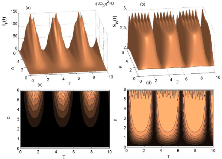
Figure 1: The volution of (a,c) Fisher’ information $I_{F}(t)$, (b,d) Wehrl’s entropy $S_{W}(t)$, versus the scaled time $T=\lambda t$ and the root of the mean photon number $\alpha=\sqrt{\bar{n}}$.

We start now the presentation of our numerical results. We will see that the coherent state parameter $\alpha$, representing the square root of the mean-photon number, greatly influences the dynamics, as can be clearly appreciated in Figs. 1 that depict, respectively, $I_{F}$ and $S_{W}$ as a function of $T$ and $\alpha$ [(a) and (b)] together with their projections on the $\alpha-T-$plane [(c) and (d)] ($T$ is a “scaled” time). Both the inherent periodicity of the dynamics and the long living correlation between the single qubit and the coherent field are clearly visible. They increase as the phonon-number grows. Both quantifiers exhibit the periodicity of the system.

In figure 2 we plot the FI- and Wehrl- time evolutions together with the associated $Y-$variance. For typographical simplicity, we set in the graphs $Y\equiv X_{2}.$ One chooses three values of the $\alpha-$parameter, namely, $=1,2,3$, respectively. In order to ensure good accuracy, the behavior of the Fisher information $I_{F}(t)$ has been determined using an appropriate scale so as to meaningfully compare it to Wehrl’s entropy. FI’s behavior is clearly dominated by the variance component $\sigma_{X_{2}}^{2}(t)$ [Cf. Eq. 11].

Fig. 3 illustrates the $I_{F}$ vs. $S_{W}$ behavior, which is surprising indeed. The second is a global measure, while the former is a local one [48]. One expects them to behave in opposite fashion [48]. Here though, a monotonous comportment is apparent, for the first time as far as we know. Rapid fluctuations, combined with strong delocalization are thus generating a bizarre scenario. There is more to be said, though. Wherl’s entropy was invented as a measure of delocalization in phase-space. For the minimum possible mean photon number (corresponding to $\alpha=1$), quantum indeterminacy is maximal and both quantifiers grow together. We may understand this behavior if we realize that, as indeterminacy augments (and so does $S_{W}$) fluctuations rise, forcing $I_{F}$ to increase as well. Enters now a bit of rather interesting physics. The route to classicality is paved by i) a growing mean photon-number and ii) a stabilization of Wehrl’s entropy since delocalization stops augmenting. This scenario begins to insinuate itself at $\alpha=2$ and becomes fully installed already at $\alpha=3$! Thus, $S_{W}$ cannot grow, but nothing impedes $I_{F}$ to increase. What we are really watching in Fig. 3-(c) is the emergence of the classical limit.

The above considerations receive a boost via Fig. 4, that depicts the FIM-Wehrl behavior versus the mean phonon number. In a sense, things return to “normality”, as the quantifiers behave differently here, as expected. $I_{F}$ always grows with $\alpha$ entailing that, as one intuitively understands, errors diminish as particle-number grows. Wherl’s measure has a peak at about $\alpha=3$. This can also be understood. $S_{W}$ measures our ignorance about localization in phase-space, which, as it should, diminishes as $\alpha$ grows.

3.1 Cramer-Rao bound

The “true” FI-informational content is conveyed by the Cramer-Rao inequality (CR). Indeed, this is its most important property. We recapitulate in one-dimension, for simplicity’s sake. If the classical Fisher information associated with translations of a one-dimensional observable $x$ with corresponding probability density $f(x)$ is [28, 46]

$$I_{x}=\int\mathrm{d}x\,f(x)\,\left(\frac{\partial\ln f(x)}{\partial x}\right)^{2},$$ (17)

then it obeys the above referred inequality, namely

$$(\Delta x)^{2}\geq I_{x}^{-1}$$ (18)

involving the variance of the stochastic variable $x$ [46]

$$(\Delta x)^{2}=\langle x^{2}\rangle-\langle x\rangle^{2}=\int\mathrm{d}x\,f(x)\,x^{2}-\left(\int\mathrm{d}x\,\rho(x)\,x\right)^{2}.$$ (19)

We remark that the derivative operator significantly influences the contribution of minute local $f-$variations to FI’s value, so that the quantifier is called a “local” one. Note that Wehrl’s entropy decreases with skewed distributions, while Fisher’s information increases in such a case. Local sensitivity is useful in scenarios whose description necessitates appeal to a notion of “order”. For our present purposes we deal with a time-dependent CR, that, in self-explanatory notation reads

$$I_{F}(t)\Delta_{t}^{2},$$

where

$$\left.\begin{array}[]{c}\Delta_{t}^{2}=\left\langle\beta^{2}\right\rangle-\left\langle\beta\right\rangle^{2}\\ \left\langle\beta^{s}\right\rangle=\int_{0}^{2\pi}\int_{0}^{\infty}\left|\beta\right|^{s}Q_{F}\left(\beta,t\right)\left|\beta\right|d\left|\beta\right|d\Theta;\text{ \ \ \ \ \ \ \ \ \ \ }s=1,2,\end{array}\right.$$

and we display in Fig. 5 some results. We see that the CR product oscillates with time and rapidly decreases as $\alpha$ grows. At $\alpha=3$ the product almost reaches its lower bound of unity, reconfirming the fact that at that $\alpha-$value classicality has been reached.

4 Conclusions

We have here considered, from an information-theory viewpoint, the dynamics of a single-qubit system. Our information-quantifiers were the Wehrl entropy, a phase-space delocalization measure, and Fisher’s information. These two quantities aptly illustrate on the complicated dynamics at hand. The main characteristics of the problem are governed by the mean phonon number and the intensity dependent field.

We have performed an extensive numerical analysis, illustrated via a variety of graphs. Periodicity is a main feature, specially as the mean-phonon number grows. Long living correlations between the qubit system and and coherent field are clearly appreciated. The monotonous growing of the Fisher measure as the Wehrl entropy grows is a counterintuitive feature that we have detected. This is a surprising facet because it is well known that whenever Fisher grows, Shannon or Wehrl entropies decrease [28, 44]. Notice that FI measures gradient content [28, 44] while Wehrl’s measure is a delocalization-indicator [44]. However, the physics of the phenomenon can be understood, as explained in the preceding Section. Rather unexpectedly, we get illuminating insights into the emergence of classicality, in line with very recent findings [47].

Figure 2: Time volution of (a) Fisher’ information $I_{F}(t)$, (b) Wehrl’s entropy $S_{W}(t)$, and (c) variances $\sigma_{X_{2}}^{2}(t)$. We set $Y\equiv X_{2}$. We also plot curves for different values of the square root of the mean photon number $\alpha,$ namely, dotted curve for $\alpha=1$, dashed curve for $\alpha=2$, and solid curve for $\alpha=3$.

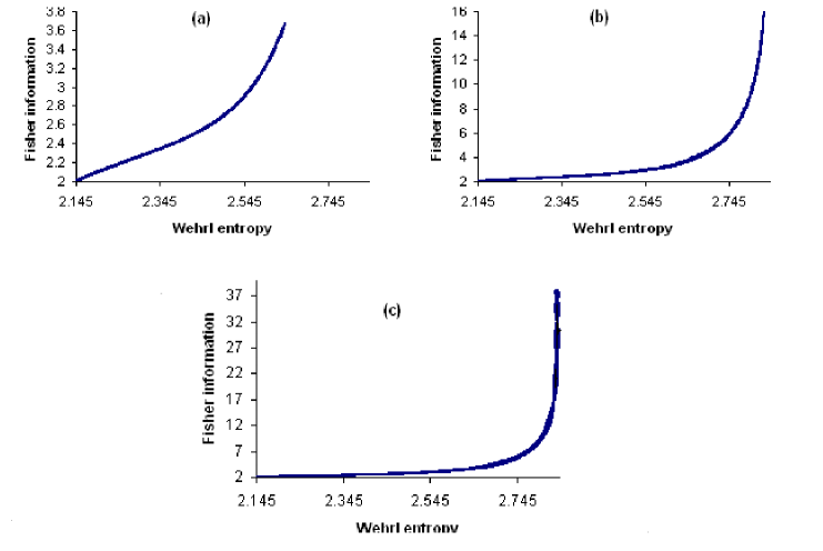
Figure 3: Illustration of the $I_{F}$ vs. $S_{W}$  behavior for parameters values for different values of  the square root of $\alpha$, where figure (a) $\alpha=1$, figure (b) $\alpha=2$, and $\alpha=3$ for figure (c).

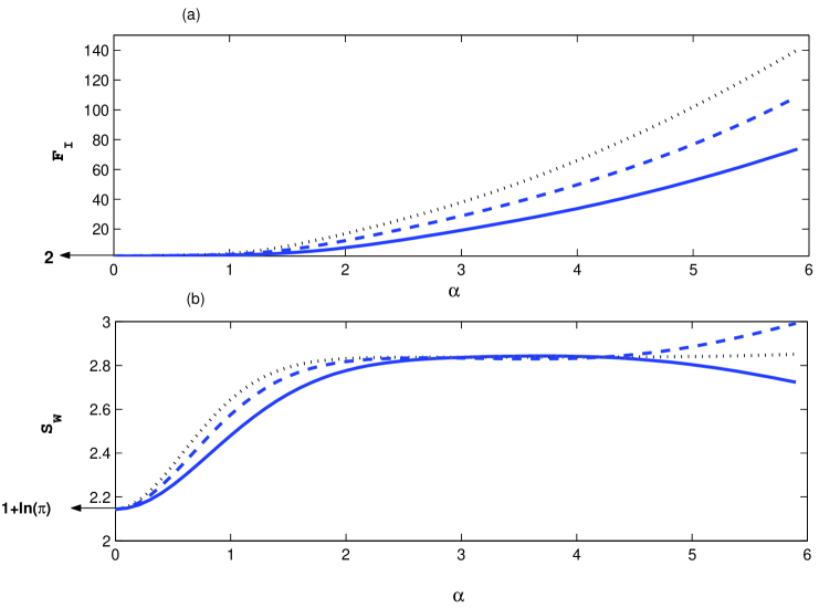
Figure 4: We depict the FIM-Wehrl behaviors versus the square root of the mean photon number.

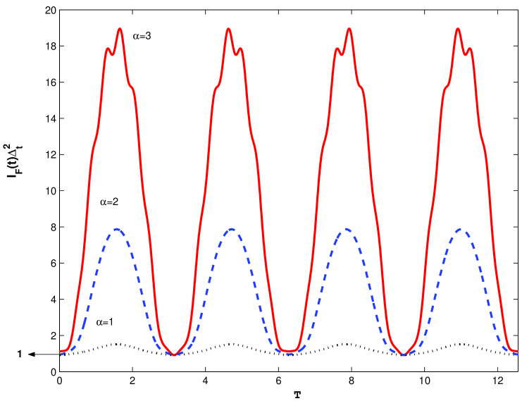
Figure 5: The Cramer-Rao product $I_{F}(t)\Delta_{t}^{2}$ as a function of the scaled time $T$  for different values of  $\alpha$ where the dotted curve $\alpha=1$, dashed curve $\alpha=2$ and the solid curve $\alpha=3$.

References

- [1] E.T. Jaynes, F.W.Cummings, IEEE 51, 89 (1963).
- [2] B.W. Shore, P.L. Knight, J. Mod. Opt. 40, 1195 (1993).
- [3] B. Buck, C.V. Sukumar, Phys. Lett. A 81, 132 (1981).
- [4] K. Zaheer, M.R.B. Wahiddin, J. Mod. Opt. 41. 150 (1994).
- [5] D. S. Freitas, A. Vidiella-Barranco and J. A. Roversi, Physics Letters A 249, 275 (1998).
- [6] J. von Neumann, Mathematical Foundations of Quantum Mechanics (Princeton University Press, Princeton (NJ), 1955).
- [7] G. Manfredi, M. R. Feix, Phys. Rev. E 62, 4665 (2000).
- [8] C. E. Shannon and W. Weaver The Mathematical Theory of Communication (Urbana University Press, Chicago, 1949).
- [9] A. Wehrl, Rev. Mod. Phys. 50 , 221(1978); Rep. Math. Phys., 30, 119 (1991).
- [10] V. Bužek, C. H. Keitel, P. L. Knight, Phys. Rev. A 51, 2575 (1995); j. B. Watson et al. Phys. Rev. A 54, 729 (1996).
- [11] A. Anderson, J. J. Halliwell Phys. Rev. D 48, 2753 (1993).
- [12] A. Orlowski, H. Paul and G. Kastelewicz Phys. Rev. A 52, 1621 (1995).
- [13] A. Miranowicz, H. Matsueda and M. R. B. Wahiddin J. Phys. A: Math. Gen. 33, 5159 (2000); A. Miranowicz et al. J. Phys. A: Math. Gen. 34, 3887 (2001).
- [14] A-S F. Obada, S. Abdel-Khalek J. Phys. A: Math. Gen. 37, 6573 (2004).
- [15] S. Abdel-Khalek, Physica A 387, 779 (2008).
- [16] S. Abdel-Khalek, Phys. Scr. 80, 045302 (2009).
- [17] R. A. Fisher, Proc. Cambridge Philos. Soc. 22, 700 (1925).
- [18] F. Pennini, A. Plastino, Phys. Rev. E 69, 057101 (2004).
- [19] F. Pennini, A. Plastino, Phys. Lett. A 326, 20 (2004).
- [20] F. Pennini, A. Plastino, G. L. Ferri, F. Olivares, Phys. Lett. A 372, 4870 (2008).
- [21] Z. Hradil, J. J. Rehacek, Phys. Lett. A 334, 267 (2005).
- [22] A.-S. F. Obada, S. Abdel-Khalek, Physica A 389, 891 (2010).
- [23] S. Abdel-Khalek, Int. J. of Quantum Information 7, 1541 (2009).
- [24] A. -S. F. Obada, S. Abdel-Khalek, A. Plastino, Physica A, 390 , 525 (2011).
- [25] J. Batle, A. R. Plastino, M. Casas, A. Plastino, Phys. Lett. A 318, 506 (2003).
- [26] J. Batle, M. Casas, A. R. Plastino, A. Plastino, Int. J. of Quantum Information, 3, 99 (2005).
- [27] J. Batle, M. Casas, A. Plastino, A.R. Plastino, Phys. Rev. A 71, 024301 (2005).
- [28] B. R. Frieden, Physics from Fisher information, (Cambridge University Press, Cambridge, 1998); Science from Fisher information (Cambridge University Press, Cambridge, 2004).
- [29] D. A. Lavis, R. F. Streater, Studies in the History and Philosophy of Modern Physics 33, 327 (2002).
- [30] V Kapsa, L Skala, J. Chen Physica E 42, 293 (2010).
- [31] B. R. Frieden, B. H. Soffer Physica A 388, 1315 (2009).
- [32] M R Ubriaco, Phys. Lett. A 373, 4017 (2009).
- [33] S Lopez-Rosa, J C Angulo, J S Dehesa, R J Yanez, Physica A 387, 2243 (1998).
- [34] S. P. Flego, F. Olivares, A. Plastino, M. Casas, Entropy 13, 184 (2011).
- [35] K. D. Sen, J. Antolin, J C Angulo, Phys. Rev. A 76, 032502 (2007).
- [36] A Nagy, Chem. Phys. Lett. 449, 212 (2007).
- [37] A Nagy, Chem. Phys. Lett. 425, 154 (2006).
- [38] S Curilef, F Pennini, A Plastino, G L Ferri, J. Phys. A 134, 012029 (2008).
- [39] A Hernando, C Vesperinas, A Plastino, Physica A 389, 490 (2010).
- [40] A Hernando, C Vesperinas, A Plastino, Phys. Lett. A 374, 18 (2009).
- [41] F Pennini, G L Ferri, A Plastino, Entropy 11, 972 (2009). (1998) 498.
- [42] F Olivares, F Pennini, A Plastino, Physica A 389, 2218 (2010).
- [43] F Pennini, A Plastino, B H Soffer, C Vignat, Phys. Lett. A 373, 817 (2009).
- [44] F. Pennini, A. Plastino, Phys. Rev. E 69, 057101 (2004).
- [45] F. Pennini, A. Plastino, Phys. Lett. A 326, 20 (2004).
- [46] M. J. W. Hall, Phys. Rev. A 62, 012107 (2000); A. L. Mayer, C. W. Pawlowski, H. Cabezas, Ecological Modeling 195, 72 (2006).
- [47] Xia-Ji Liu, Hui Hu, P. D. Drummond, Phys. Rev. A 82, 023619 (2010).
- [48] F. Pennini, A. Plastino Phys. Lett. A 365, 263 (2007).