IPhT-T11/014

On Type IIB moduli stabilization and
${\cal N}=4,8$ supergravities
Gerardo Aldazabal^a,b, Diego Marqués^c, Carmen Núñez^d and
José A. Rosabal^a
aCentro Atómico Bariloche, ^bInstituto Balseiro (CNEA-UNC) and CONICET
8400 S.C. de Bariloche, Argentina.
^c Institut de Physique Théorique, CEA/ Saclay
91191 Gif-sur-Yvette Cedex, France
^dInstituto de Astronomía y Física del Espacio (CONICET-UBA) and
Departamento de Física, FCEN, Universidad de Buenos Aires
C.C. 67 - Suc. 28, 1428 Buenos Aires, Argentina
Abstract

We analyze $D=4$ compactifications of Type IIB theory with generic, geometric and non-geometric, dual fluxes turned on. In particular, we study ${\cal N}=1$ toroidal orbifold compactifications that admit an embedding of the untwisted sector into gauged ${\cal N}=4,\ 8$ supergravities. Truncations, spontaneous breaking of supersymmetry and the inclusion of sources are discussed. The algebraic identities satisfied by the supergravity gaugings are used to implement the full set of consistency constraints on the background fluxes. This allows to perform a generic study of ${\cal N}=1$ vacua and identify large regions of the parameter space that do not admit complete moduli stabilization. Illustrative examples of AdS and Minkowski vacua are presented.

1 Introduction

Compactifications of superstring theory to four dimensions must be addressed if a link between string theory and the physics of the observable world is to be established. From a phenomenological approach, the compactification process must fulfill some very basic requirements. For instance, part of the original supercharges must be projected out in order to obtain a $D=4$ phenomenologically acceptable ${\cal N}=1$ supersymmetric (or ${\cal N}=0$) theory and a chiral fermionic spectrum must be allowed. These requirements are linked to the structure of the internal manifold and to the presence of sources like D-branes or orientifold planes. Clearly, other kinds of compactifications with more supersymmetry charges are also worth being studied in order to explore other aspects of the theory like, for example, the AdS/CFT correspondence.

In a generic compactification, field strength background fluxes for the different form fields can be turned on. An appealing feature of these so called flux compactifications [1, 2] is that scalar fields, which would be moduli in the absence of fluxes, acquire a potential [3] and thus, vacuum degeneracy can be lifted. Unfortunately, a string theory formulation of compactifications with fluxes is not yet available and we must tackle them by using the low energy effective supergravity theory. More precisely, superstring flux compactifications would be described by gauged supergravities [4]-[9], namely, deformations of ordinary abelian supergravity theories where the deformation parameters (gaugings) correspond to the quantized fluxes [10]-[14]. Consistency constraints on gaugings are needed for the supergravity theory to be well defined [2].

The connection between a string compactification and the gauged supergravity effective theory is not fully evident and calls for some interpretation. In fact, a first sight inspection seems to indicate that there are many more gaugings available than background fluxes. For instance, an orientifold compactification with fluxes of the Type IIB supergravity action (the low energy effective theory of Type IIB superstrings), leads to a $D=4$, ${\cal N}=4$ supergravity theory involving only a small subset of all possible gaugings (identified with Type IIB 3-form fluxes). An explanation of this missmatch relies in the fact that, starting with the effective $D=10$ theory, one is missing some key stringy ingredients like, for instance, T-duality invariance. Actually, if different dualities (like T-duality, IIB S-duality, M-theory or heterotic/Type I S-duality), expected from the underlying string theory, are enforced in the low energy four dimensional action, new “dual fluxes” must be invoked, and a one to one correspondence between gaugings and fluxes can be established [15, 16]. A way to accomplish this correspondence is to compare the (orbifold projected) gauged supergravity algebra with the duality completion of the algebra satisfied by compactified $D=10$ vector bosons (see [13, 14]). Interestingly enough, the Jacobi identities (JI) of the resulting algebra encode the constraints that dual fluxes must obey, including and generalizing the already known Bianchi identities and tadpole cancelation equations. In this interpretation, the four dimensional supergravity theory integrates information about the stringy aspects of the starting configuration and it is not just the reduction of a ten dimensional effective supergravity action.

It must be recalled, however, that even if this correspondence is established, the interpretation in terms of $D=10$ fields is subtle. In particular, non geometric fluxes must be incorporated, meaning that globally matching solutions requires, besides diffeomorphisms and gauge invariance, T or S-duality (or generically U-duality) transformations as part of the transition functions. The concept of Generalized Geometry has been proposed as an appealing framework to describe flux compactifications [17].

Here we study ${\cal N}=1$ supergravity models resulting from orbifold compactification with fluxes. Our starting point is the framework of [13] where Type IIB orientifold compactifications plus a $\mathbb{Z}_{2}\times\mathbb{Z}_{2}$ orbifold projection ensuring tori factorization are considered. The goal of the paper is twofold. On the one hand we analyze the conditions under which the untwisted sectors of such string theories correspond to truncations of gauged supergravities. These consistency conditions are then used to implement the full set of constraints on fluxes. Some of these constraints have not received much attention previously. We finally solve all the consistency equations for fluxes and analyze their impact in the analysis of moduli fixing.

In the absence of sources, the untwisted sector of such compactification is just the orbifold projection of an underlying ${\cal N}=4$ gauged supergravity theory. This sector was first found in [16], were it was shown that $2^{7}$ dual fluxes are needed to ensure duality invariance. In [13], a subset of $2^{6}$ fluxes was shown to describe globally non-geometric compactifications of F-theory (which admit a geometric local description in terms of $D=10$ supergravity) and a consistent procedure for incorporating F-theory seven branes into the gauge algebra was discussed. Moreover, the algebra of gauge generators and JI leading to constraints on fluxes were derived, and shown to coincide with that of ${\cal N}=4$ gauged supergravity, when there are no sources.

In Section 2, we start introducing some essential features of Type IIB/O3 orientifolds, their moduli space and effective action in the presence of the complete set of fluxes allowed by the orbifold.

We begin Section 3 with a review of basic notions on gauged ${\cal N}=4$ supergravity, relevant for our discussion. We then analyze the “shift matrices” and the scalar potential of gauged ${\cal N}=4$ supergravity. We discuss the projection to ${\cal N}=1$ and a scheme for spontaneous supersymmetry breaking solutions. We also consider the possibility of embedding the model into an underlying ${\cal N}=8$ gauged supergravity theory, and derive new constraints on dual fluxes. The analysis is completed with a discussion about the incorporation of sources. The full analysis allows us to understand the embedding of the string effective action in gauged supergravity and the link between fields, parameters, constraints, etc.

Section 4 is devoted to a generic analysis of moduli fixing in Type IIB orbifolds (possibly including three and seven branes). The complete set of physical and algebraic constraints on moduli and fluxes is reviewed and an exclusion principle allowing to identify models that do not admit full moduli stabilization is formulated. We use this result to determine large regions of the parameter space that are excluded, and focus on models with potentiality to fully stabilize all moduli. Illustrative examples of SUSY vacua are presented.

Finally, Section 5 presents some conclusions and an outlook. We collect in the Appendices some useful equations and tables containing fluxes and their transformation properties.

2 Type IIB/O3 ${\cal N}=1$ compactifications with generic fluxes

We consider Type IIB/O3 orientifold compactifications on $T^{6}/[\Omega_{P}(-1)^{F_{L}}\sigma\times\Gamma]$, where $\Omega_{P}$ is the worldsheet parity operator, $(-1)^{F_{L}}$ is the space-time fermionic number for left-movers and $\sigma$ is an involution operator acting on internal coordinates as $\sigma(x^{i})=-x^{i}$. $\Gamma$ is an orbifold projection to be specified below. We introduce a basis of 3-forms for this space

$$\alpha_{0}=dx^{1}\wedge dx^{2}\wedge dx^{3}\ ,\ \ \ \ \ \ \alpha_{i}^{\ j+3}=\frac{1}{2}\epsilon_{ilm}dx^{l}\wedge dx^{m}\wedge dx^{j+3}\,,$$

$$\beta^{0}=dx^{4}\wedge dx^{5}\wedge dx^{6}\ ,\ \ \ \ \ \ \beta^{i}_{\ j+3}=-\frac{1}{2}\epsilon_{jlm}dx^{l+3}\wedge dx^{m+3}\wedge dx^{i}\,,$$ (2.1)

with elements normalized according to $\int dx^{1}\wedge\dots\wedge dx^{6}=1$. In addition, we take the basis of closed 2-forms and their $\ast_{6}$-dual 4-forms as

$$\omega_{ij}=-dx^{i}\wedge dx^{j+3}\ ,\ \ \ \ \ \ \tilde{\omega}_{ij}=\frac{1}{4}\ \epsilon_{ilm}\epsilon_{jpq}\ dx^{l}\wedge dx^{p+3}\wedge dx^{m}\wedge dx^{q+3}\,.$$ (2.2)

We define a complex structure whose deformations are controlled by complex structure moduli $U^{m}_{\ \ n}$

$$\Omega=dz^{1}\wedge dz^{2}\wedge dz^{3}\ ,\ \ \ \ dz^{m}=dx^{m}+iU^{m}_{\ \ p}dx^{p+3}\,,$$ (2.3)

and a complexified Kähler 4-form with Kähler moduli $T^{ij}$

$${\cal J}_{c}\equiv C_{4}+\frac{i}{2}e^{-\phi}J\wedge J=iT^{ij}\tilde{\omega}_{ij}\ .$$ (2.4)

Finally, the RR axion and the string coupling combine into the axion-dilaton modulus as

$$S=e^{-\phi}+iC_{0}\,.$$ (2.5)

The $1+9+9$ complex moduli span a Kähler manifold with Kähler potential [18]

$$K = -\log(S+\bar{S})-\log\left[-i\int\Omega\wedge\bar{\Omega}\right]-2\log\left[\frac{1}{6}\int J\wedge J\wedge J\right]$$ (2.6)

$$= -\log[(S+\bar{S})\det(U+\bar{U})\det(T+\bar{T})]\,.$$

For trivial $\Gamma$, this orientifold leads to ${\cal N}=4$ effective theories in $D=4$ (see [19]). The large amount of SUSY can be broken in particular to ${\cal N}=1$ by orbifolding the theory with a discrete symmetry group $\Gamma\subset SU(3)$. In this case the structure group of the tangent bundle is still the trivial one, but it is enhanced to $SU(3)$ at the orbifold fixed points. Then, two different sectors of states can be distinguished. The untwisted sector is given by direct truncation of the parent ${\cal N}=4$ theory and its $SL(2,\mathbb{Z})\times SO(6,6;\mathbb{Z})$ gauge group, while the twisted states localized at the orbifold singularities transform under a larger symmetry group. In this work we restrict to the untwisted sector. We consider $\Gamma=\mathbb{Z}_{2}\times\mathbb{Z}_{2}$, which orbifolds the internal space as

	$x^{1}$	$x^{2}$	$x^{3}$	$x^{4}$	$x^{5}$	$x^{6}$
$\mathbb{Z}_{2}$	$-$	$-$	$+$	$-$	$-$	$+$
$\mathbb{Z}_{2}$	$+$	$-$	$-$	$+$	$-$	$-$

leaving only the diagonal Kähler and complex moduli $T_{i}=T^{ii}$ and $U_{i}=U^{i}_{\ i}$, which leads to

$$K=-\log(S+\bar{S})-\sum_{i=1}^{3}\log(U_{i}+\bar{U}_{i})-\sum_{i=1}^{3}\log(T_{i}+\bar{T}_{i})\,.$$ (2.7)

After orbifoldization, the global symmetry group associated to the moduli space of the internal manifold is $SL(2,\mathbb{Z})^{7}$, where each $SL(2,\mathbb{Z})$ generates modular transformations for each of the seven moduli $S$, $U_{i}$ and $T_{i}$. These fields can be grouped in the vector representation $\mathbb{T}\equiv\mathbf{7}=(S;T_{1},T_{2},T_{3};U_{1},U_{2},U_{3})$ and the flux parameters transform in the spinorial representation $\mathbb{G}\equiv\mathbf{128}$ [16], each flux being characterized by a given set of Weyl spinors $(\pm,\pm,\pm,\pm,\pm,\pm,\pm)$ (see [13] for details on the spinor formalism).

In the absence of fluxes, any moduli configuration corresponds to a possible vacuum in which all fields are massless. The orientifold involution allows to turn on RR $F_{3}$ and NSNS $H_{3}$ background fluxes, which lift the moduli space generating a superpotential [3]

$$W=\int(F_{3}-iSH_{3})\wedge\Omega\,.$$ (2.8)

Clearly, this superpotential cannot fully stabilize all moduli (in particular, it is independent of $T_{i}$). However, string dualities can be invoked to construct an effective four dimensional theory in which $W$ depends on all the moduli, being the low energy limit of a ten dimensional string set up, rather than ten dimensional supergravity. To achieve this commitment, one can promote T-duality and S-duality to symmetries of the four dimensional theory. For example, in order to restore mirror symmetry between IIA/IIB orientifold compactifications, new set of fluxes were introduced in [15]-[16]. T-duality was used to connect the $H_{3}$ fluxes with non-geometric fluxes through the chain

$$H_{mnp}{\stackrel{{\scriptstyle{\rm T}_{m}}}{{\longleftrightarrow}}}-\omega^{m}_{np}{\stackrel{{\scriptstyle{\rm T}_{n}}}{{\longleftrightarrow}}}-Q^{mn}_{p}{\stackrel{{\scriptstyle{\rm T}_{p}}}{{\longleftrightarrow}}}R^{mnp}\ .$$ (2.9)

Some of these new objects were given a clear interpretation: the geometric $\omega$ fluxes correspond to structure constants of compactifications on twisted tori [20] and the $Q$-fluxes correspond to locally geometric but globally non-geometric constructions [21]. The $R$ fluxes instead, correspond to highly non-geometric compactifications, not even admitting a local description [15]. Only the $H$ and $Q$ fluxes survive the orientifold projection and many of their components vanish after modding by the $\Gamma$ symmetry. Under S-duality, the axion-dilaton transforms as

$$S\to\frac{kS-i\ell}{imS+n}\ ,\ \ \ \ kn-lm=1\,,$$ (2.10)

and the 3-form fluxes rotate as doublets

$$\left(\begin{matrix}F_{3}\\ H_{3}\end{matrix}\right)\rightarrow\left(\begin{matrix}k&\ell\\ m&n\end{matrix}\right)\left(\begin{matrix}F_{3}\\ H_{3}\end{matrix}\right)\,.$$ (2.11)

In [16] the $Q$-fluxes were included in the superpotential, and in order to achieve S-invariance, a new set of fluxes $P^{ij}_{k}$ was considered. They both conform an $SL(2,\mathbb{Z})$-doublet

$$\left(\begin{matrix}Q\\ P\end{matrix}\right)\rightarrow\left(\begin{matrix}k&\ell\\ m&n\end{matrix}\right)\left(\begin{matrix}Q\\ P\end{matrix}\right)\,.$$ (2.12)

Since the $SL(2,\mathbb{Z})$ symmetry relating these fluxes is a symmetry of the Type IIB supergravity equations of motion, the $P$-flux parameters are expected to correspond to compactifications admitting a ten dimensional local supergravity description. The full superpotential is

$$W=\int[(F_{3}-iSH_{3})+(Q-iSP){\cal J}_{c}]\wedge\Omega\ ,\ \ \ \ \ \ (Q{\cal J}_{c})_{p_{1}p_{2}p_{3}}=\frac{1}{2}Q^{ab}_{[p_{1}}({\cal J}_{c})_{p_{2}p_{3}]ab}\ .$$ (2.13)

Finally, by further demanding the four dimensional effective theory to be invariant under $SL(2,\mathbb{Z})^{7}$, new “primed” fluxes must be incorporated [16]. Then, the full invariant (modulo Kähler transformations) superpotential reads

$$W=\int(f_{+}-iSf_{-})\cdot e^{{\cal J}_{c}}\wedge\Omega\,,$$ (2.14)

where $f_{\pm}$ denote the formal sums

$$f_{+}=F_{abc}+Q^{ab}_{c}+Q^{\prime a}_{bc}+\tilde{F}^{\prime abc}\ ,\ \ \ \ \ \ f_{-}=H_{abc}+P^{ab}_{c}+P^{\prime a}_{bc}+\tilde{H}^{\prime abc}\,.$$ (2.15)

Tilded and untilded 3-forms are related as $\tilde{F}^{ijk}\equiv\frac{1}{3!}\epsilon^{ijkopq}F_{opq}$.

Besides (2.13), we have defined the 3-forms

$$(Q^{\prime}\cdot{\cal J}_{c}^{2})_{p_{1}p_{2}p_{3}} = \frac{1}{32}Q^{\prime a}_{[p_{1}p_{2}}({\cal J}_{c})_{p_{3}]ai_{1}i_{2}}({\cal J}_{c})_{i_{3}i_{4}p_{5}p_{6}}\epsilon^{i_{1}i_{2}i_{3}i_{4}i_{5}i_{6}}\,,$$ (2.16)

$$(\tilde{F}^{\prime}\cdot{\cal J}_{c}^{3})_{p_{1}p_{2}p_{3}} = \frac{5}{128}\tilde{F}^{\prime abc}({\cal J}_{c})_{[p_{1}p_{2}p_{3}a}({\cal J}_{c})_{bc]i_{1}i_{2}}({\cal J}_{c})_{i_{3}i_{4}i_{5}i_{6}}\epsilon^{i_{1}i_{2}i_{3}i_{4}i_{5}i_{6}}\,.$$ (2.17)

An expanded version of the superpotential in terms of flux parameters can be found in Appendix A (we do not include contributions from twisted sectors, which are also expected).

Although the effective potential that we have just motivated looks rather generic, its parameters are strongly constrained by consistency requirements. From a higher dimensional point of view these constraints originate, for instance, in Bianchi identities and anomaly cancelation conditions. An efficient way of finding such constraints was proposed in [13] by constructing a full invariant algebra through systematic application of $SL(2,{\mathbb{Z}})^{7}$ dualities on the well known algebra of gauge generators associated to non-geometric Type IIB fluxes. We summarize the results of [13] in Appendix A, and extend them by including also “primed” fluxes.

For particular sets of fluxes, the untwisted scenario that we have just described corresponds to a truncation of gauged ${\cal N}=4$ supergravity [13]. In the following section we show that this holds in general, and stress the connection between orbifold compactifications of string theory and gauged supergravity truncations.

3 Gauged ${\cal N}=4,\ 8$ supergravity embeddings

The full $SL(2,\mathbb{Z})^{7}$ duality group of the untwisted sector of the ${\cal N}=1$ theory discussed in the previous section is just the orbifold projection of the $SL(2,\mathbb{Z})\times SO(6,6;\mathbb{Z})$ global symmetry group of gauged ${\cal N}=4$ supergravity. Therefore we expect the untwisted sector of the $D=4$ effective action to correspond to a truncation of a gauged ${\cal N}=4$ supergravity, and the full set of fluxes to correspond to all possible gaugings in [15]. Actually, this connection was analyzed for a subset of gaugings of Type IIB in [13] and of Type IIA in [14]. Here we further elaborate and generalize this connection to the full set of gaugings allowed by the orbifold.

We begin by reviewing gauged ${\cal N}=4$ supergravity [8], focusing the attention on the scalar sector, consistency constraints and supersymmetry variations of the fermions. We analyze orbifold truncations of these theories, and their link to orbifold compactifications in string theory (with and without sources). Spontaneous supersymmetry breaking is also discussed.

3.1 Gauged ${\cal N}=4$ supergravity truncations

Let us start by collecting some known facts about ${\cal N}=4$ gauged supergravity that are needed for our discussion (see [8] for details). These theories have $1+9+9+...$ complex scalars $S\ +\ U^{m}{}_{\tilde{q}}\ +\ T^{l\tilde{m}}\ +\ ...$ that span the coset

$$\frac{SL(2)|_{B}}{U(1)}\times\frac{SO(6,6+n)}{SO(6)\times SO(6+n)}\,.$$ (3.1)

The first factor in the coset can be parameterized by the metric $M^{\alpha\beta}={\rm Re}[{\cal V}^{\alpha}{\cal V}^{\beta*}]$ with

$${\cal V}^{\alpha}=\frac{1}{\sqrt{s_{x}}}\left(\begin{matrix}1\\ -i{S}\end{matrix}\right)\ ,\ \ \ \ \ M^{\alpha\beta}=\frac{1}{s_{x}}\left(\begin{matrix}1&{s_{y}}\\ {s_{y}}&|S|^{2}\end{matrix}\right)\,,\quad\quad$$ (3.2)

where $S=s_{x}+is_{y}$. The second factor is characterized by the vielbeins ${\cal V}^{a}$ and ${\cal V}^{m}$ with $m=1,\dots,6$ and $a=7,\dots,12+n$ and the coset can be parameterized by the metric

$$M_{MN}=({\cal V}{\cal V}^{T})_{MN}\,,$$ (3.3)

where capital indices take values $M,N,...=1,\dots,12+n$ such that the first six indices run over the rank of the $SO(6)$ factor whereas the other values run over the rank of the $SO(6+n)$ factor (in this paper we will mainly restrict to $n=0$).

Supersymmetry and anomaly cancelation require a potential for the scalars living in the vector multiplets, namely

$$V_{\mathcal{N}=4}=\frac{1}{16}\left[f_{\alpha MNP}f_{\beta QRS}M^{\alpha\beta}\left(\frac{1}{3}M^{MQ}M^{NR}M^{PS}+\left(\frac{2}{3}\eta^{MQ}-M^{MQ}\right)\eta^{NR}\eta^{PS}\right)\right.\\ \left.-\frac{4}{9}f_{\alpha MNP}f_{\beta QRS}\epsilon^{\alpha\beta}M^{MNPQRS}+3\xi_{\alpha}^{M}\xi_{\beta}^{N}M^{\alpha\beta}M_{MN}\right]\,,$$ (3.4)

together with a topological term for the vector fields [8]. Here $M^{MNPQRS}$ is a completely antisymmetric tensor which can be expressed in terms of the vielbeins as

$$M^{MNPQRS}=\epsilon^{mnpqrs}{\cal V}_{m}^{\ \ M}{\cal V}_{n}^{\ N}{\cal V}_{p}^{\ P}{\cal V}_{q}^{\ Q}{\cal V}_{r}^{\ R}{\cal V}_{s}^{\ S}\,,$$ (3.5)

and the indices are lowered and raised with the off diagonal $SO(6,6)$ metric

$$\eta^{MN}=\eta_{MN}=\left(\begin{array}[]{cc}0&I_{6\times 6}\\ I_{6\times 6}&0\end{array}\right)\ ,\ \ \ \ \ \ \ \eta^{MN}={\cal V}_{P}{}^{M}\,\eta^{PQ}\,{\cal V}_{Q}{}^{N}\ .$$ (3.6)

The embedding tensors $f_{\alpha MNP}$ and $\xi_{\alpha M}$ with $\alpha=\pm 1/2$ and $M=1\ldots 12+n$, encode all possible gaugings of $\mathcal{N}=4$ supergravity, with $n$ extra vector multiplets of $SL(2,\mathbb{Z})\times SO(6,6+n;\mathbb{Z})$. For $n=0$ they live in $(\mathbf{2},\mathbf{220})$ and $(\mathbf{2},\mathbf{12})$ representations, respectively. In what follows, we will not include the $\xi_{\alpha M}$ fluxes, which are projected out by the orbifold.

Consistency requires the gaugings to satisfy several constraints that can be obtained from the algebra of gauge generators, namely [8]

$$\left[Z_{\alpha A},Z_{\beta B}\right]=f^{P}_{\alpha AB}\ Z_{\beta P}=f^{P}_{\beta AB}\ Z_{\alpha P}\,,$$ (3.7)

where the last equality is enforced to ensure the antisymmetry of the commutator. The quadratic constraints imposed for algebraic consistency are

$$f_{\alpha[AB}^{P}f_{\beta CD]P}=0\,,\qquad\epsilon^{\alpha\beta}f_{\alpha AB}^{P}f_{\beta CDP}=0\,.$$ (3.8)

We will refer to the last set of equations as “antisymmetry conditions”. We will see later that their imposition plays a crucial role in moduli fixing, a fact that was also noted in [22].

In order to study truncations or spontaneous supersymmetry breakings, it appears enlightening to look at the quadratic terms involving fermions in the supergravity Lagrangian and the fermionic transformations under supersymmetry. With this in mind, it proves useful to work with the $SU(4)$ covering group rather than with $SO(6)$. Thus, in particular, an $SO(6)$ vector basis $e^{m}$, $m=1,\dots 6$, can be expressed in terms of a set of antisymmetric matrices $(\gamma^{m})^{ij}$, $i,j=1,\dots,4$ (details are given in Appendix B). Closely following [8] we write

$${\cal V}^{-1}{\cal L}=\dots\frac{1}{3}A_{1}^{ij}\overline{\psi}_{\mu i}\Gamma^{\mu\nu}\psi_{\nu j}-\frac{1}{3}iA_{2}^{ij}\overline{\psi}_{\mu i}\Gamma^{\mu}\chi_{j}+iA_{2ai}{}^{j}\overline{\psi}_{\mu i}\Gamma^{\mu}\lambda_{j}^{a}+h.c\dots$$ (3.9)

with ${\psi}_{\mu}^{i}$, $\chi_{j}$ and $\lambda_{j}^{a}$ the gravitini, dilatini and gaugini, respectively. The corresponding shift matrices $A_{1}$, $A_{2}$ and $A_{2a}$ are given in terms of the gaugings and the vielbeins ${\cal V}_{m}^{\ \ M}\mapsto({\cal V})^{Mij}={\cal V}_{m}^{\ \ M}(\gamma^{m})^{ij}$ by

$$A_{1}^{ij} = \epsilon^{\alpha\beta}\bar{\cal V}_{\alpha}({\cal V})^{Mik}(\overline{\cal V})^{Nkl}({\cal V})^{Plj}f_{\beta MNP}\,,$$ (3.10)

$$A_{2}^{ij} = \epsilon^{\alpha\beta}{\cal V}_{\alpha}({\cal V})^{Mik}(\overline{\cal V})^{Nkl}({\cal V})^{Plj}f_{\beta MNP}\,,$$ (3.11)

$$\overline{A}_{2ai}{}^{j} = -\epsilon^{\alpha\beta}{\cal V}_{\alpha}({\cal V})_{a}^{\ M}({\cal V})^{Nik}(\bar{\cal V})^{Pkj}f_{\beta MNP}\,.$$ (3.12)

They verify (upon use of the consistency constraints)

$$-\frac{1}{4}\delta_{j}^{i}V=\frac{1}{3}A_{1}^{ik}\bar{A}_{1jk}-\frac{1}{9}A_{2}^{ik}\bar{A}_{2jk}-\frac{1}{2}A_{2aj}{}^{k}\bar{A}_{2ai}{}^{k}\,.$$ (3.13)

The (order $g$) supersymmetry transformations of the fermions read

$$\delta\psi_{\mu}^{i} = 2D_{\mu}\epsilon^{i}-\frac{2}{3}A_{1}^{ij}\Gamma_{\mu}\epsilon_{j}\dots\,,$$ (3.14)

$$\delta\chi^{i} = -\frac{4}{3}iA_{2}^{ij}\epsilon_{j}\dots\,,$$ (3.15)

$$\delta\lambda_{a}^{i} = -2iA_{2aj}^{\ \ \ i}\epsilon^{j}\dots\,.$$ (3.16)

Now we can proceed to the orbifold projection on the scalar and fermionic sectors. The full $\xi_{\alpha M}$ is projected out, and the only surviving gaugings are

$$f_{\alpha ABC}\ ,\ \ \ \ \ \ \ A\ {\rm mod}\ 3\neq B\ {\rm mod}\ 3\neq C\ {\rm mod}\ 3\,.$$ (3.17)

Additionally, non-diagonal moduli are projected out, and only $S$, $T_{i}$ and $U_{i}$ parameterize the moduli space. The metric matrix organizes into blocks associated to each factorized torus, and reads

$$M_{i}=\frac{1}{t_{ix}u_{ix}}\left(\begin{array}[]{llll}|T_{i}|^{2}&-|T_{i}|^{2}u_{iy}&t_{iy}u_{iy}&t_{iy}\\ \\ -|T_{i}|^{2}u_{iy}&|T_{i}|^{2}|U_{i}|^{2}&-t_{iy}|U_{i}|^{2}&-t_{iy}u_{iy}\\ \\ t_{iy}u_{iy}&-t_{iy}|U_{i}|^{2}&|U_{i}|^{2}&u_{iy}\\ \\ t_{iy}&-t_{iy}u_{iy}&u_{iy}&1\end{array}\right)$$ (3.18)

where we have written the non vanishing entries in positions $M_{i}^{i+3k,i+3m}$ with $k,m=0,1,2,3$. Also, $T_{i}=t_{ix}+it_{iy}$ and $U_{i}=u_{ix}+iu_{iy}$. Each factor of the $\mathbb{Z}_{2}\times\mathbb{Z}_{2}$ orbifold action on the $SU(4)$ vectors $\widehat{e}^{i}$ (equivalent to $SO(6)$ spinors) acts according to

$$\mathbb{Z}_{2} : (\widehat{e}^{1},\widehat{e}^{2},\widehat{e}^{3},\widehat{e}^{4})\rightarrow(-\widehat{e}^{1},-\widehat{e}^{2},\widehat{e}^{3},\widehat{e}^{4})\,,$$ (3.20)

$$\mathbb{Z}_{2} : (\widehat{e}^{1},\widehat{e}^{2},\widehat{e}^{3},\widehat{e}^{4})\rightarrow(\widehat{e}^{1},-\widehat{e}^{2},-\widehat{e}^{3},\widehat{e}^{4})\,,$$ (3.21)

so that only the gravitino along the $\widehat{e}^{4}$ direction remains in the spectrum.

Comparison of the truncated algebra (3.7) with the duality completion of the flux algebra leads to the identifications [13]

$$2f_{+abp}=-F^{\prime}_{abp}\ ,\ \ \ \ \ 2f_{+ab}^{p}=Q^{\prime p}_{ab}\ ,\ \ \ \ \ 2f_{+a}^{bp}=-Q^{bp}_{a}\ ,\ \ \ \ \ 2f_{+}^{abp}=\tilde{F}^{abp}\,,$$

$$2f_{-abp}=-H^{\prime}_{abp}\ ,\ \ \ \ 2f_{-ab}^{p}=P^{\prime p}_{ab}\ ,\ \ \ \ \ \;2f_{-a}^{bp}=-P^{bp}_{a}\ ,\ \ \ \ \ 2f_{-}^{abp}=\tilde{H}^{abp}\,.$$ (3.22)

The factors 2 and signs are needed to match the normalizations of (3.4) and the scalar potential derived from the superpotential (A.4).

Let us stress that comparison of the orbifold projected scalar potential (3.4) with the scalar potential derived from the ${\cal N}=1$ superpotential (A.4) indeed shows [13] that both potentials coincide when fluxes and gaugings are identified as in (3.22) and truncated identities (3.8) are enforced (we will proceed in a similar way below to obtain ${\cal N}=8$ constraints from comparison of a truncated ${\cal N}=8$ scalar potential with the ${\cal N}=4$ potential (3.4)). The expressions that we derive below greatly simplify this comparison.

The relevant shift matrices acquire a suggestive form in terms of the full superpotential (see A.4) when written in the $SU(4)$ basis, namely

$$\begin{array}[]{ccccccc}\hskip 48.36958ptA_{1}^{44}&=&-\frac{3}{2}ie^{\frac{K}{2}}W&,&\hskip 48.36958ptA_{2}^{44}&=&\frac{3}{2}ie^{\frac{K}{2}}W(-\bar{S})\,,\\ \bar{A}_{2a4}{}^{1}(\bar{\gamma}^{a})^{14}&=&\frac{i}{2}e^{\frac{K}{2}}W(-\bar{U}_{1})&,&\bar{A}_{2a4}{}^{1}(\bar{\gamma}^{a})^{23}&=&-\frac{i}{2}e^{\frac{K}{2}}W(-\bar{T}_{1})\,,\\ \bar{A}_{2a4}{}^{2}(\bar{\gamma}^{a})^{24}&=&\frac{i}{2}e^{\frac{K}{2}}W(-\bar{U}_{2})&,&\bar{A}_{2a4}{}^{2}(\bar{\gamma}^{a})^{31}&=&-\frac{i}{2}e^{\frac{K}{2}}W(-\bar{T}_{2})\,,\\ \bar{A}_{2a4}{}^{3}(\bar{\gamma}^{a})^{34}&=&\frac{i}{2}e^{\frac{K}{2}}W(-\bar{U}_{3})&,&\bar{A}_{2a4}{}^{3}(\bar{\gamma}^{a})^{12}&=&-\frac{i}{2}e^{\frac{K}{2}}W(-\bar{T}_{3})\,,\end{array}$$ (3.23)

where $W(-\bar{\phi}_{i})$ indicates that $\phi_{i}$ must be replaced by $-\bar{\phi}_{i}$ in the argument of $W$ and all other arguments remain unchanged. In fact, the superpotential has a linear dependence on all the moduli, which guarantees that

$$(\phi_{i}+\bar{\phi}_{i})D_{\phi_{i}}W(\phi_{i})=-W(-\bar{\phi}_{i}),$$ (3.24)

where $D_{\phi_{i}}W(\phi_{i})$ is the Kähler covariant derivative and $\phi_{i}$ stands for $S,T_{i}$ or $U_{i}$. The projected shift matrices can then be written in terms of the superpotential and its Kähler derivatives, as expected. Thus, a supersymmetric vacuum solution ensures the vanishing of the covariant derivatives or, equivalently, the vanishing of the dilatini ($A_{2}$) and gaugini ($A_{2a}$) shift matrices. Such SUSY solution would be Minkowski if $A_{1}=0$ or Anti de Sitter otherwise.

3.2 Spontaneous supersymmetry breaking

The previous analysis gives us some hints for the study of spontaneous breaking of ${\cal N}=4$ to ${\cal N}=1$ supersymmetry (see [8, 14]). We must look for a fermionic direction $\epsilon^{i}$ such that $\delta\psi_{\mu}^{i}=0$, $\delta\chi^{i}=0$ and $\delta\lambda_{a}^{i}=0$ in (3.16) . Following [8], we define $\epsilon^{i}=\widehat{e}^{i}\xi$ proportional to the $SU(4)$ vector $\widehat{e}^{i}$, and then any supersymmetic vacuum configuration must obey

$$\begin{array}[]{ccccc}A_{1}^{ij}\widehat{e}_{j}=\sqrt{-\frac{3}{4}V}\widehat{e}^{i}&;&\widehat{e}_{j}A_{2}^{ji}=0&;&A_{2aj}^{\quad i}\widehat{e}^{j}=0\end{array}\,.$$ (3.25)

In particular, if we choose $i=4$, any SUSY configuration for diagonal moduli of the previously discussed orbifold truncation, would vanish along this direction if the non-diagonal moduli are set to zero and the JI (3.8) are satisfied. Such a configuration is guaranteed to correspond to a vacuum of ${\cal N}=4$. Moreover, in this situation it can be checked that the shift matrices in the remaining three directions 1, 2, 3 (which we label with indices $i,j,k$), namely

$$A^{kk}_{1} = -\frac{3}{2}i\ e^{K/2}\ W(-\bar{T}_{j},-\bar{U}_{j})\ \ \ \ \ \ \ \ \ \ \ \ \ \ \forall j\neq k\,,$$ (3.26)

$$A^{kk}_{2} = \ \ \frac{3}{2}i\ e^{K/2}\ W(-\bar{S},-\bar{T}_{j},-\bar{U}_{j})\ \ \ \ \ \ \ \ \ \forall j\neq k\,,$$ (3.27)

$$\bar{A}_{2aj}^{\ \ \ \ i}(\bar{\gamma}^{a})^{ij} = \ \ \frac{i}{2}\ e^{K/2}\ W(-\bar{U}_{i},-\bar{T}_{k})\ \ \ \ \ \ \ \ \ \ \ \ \ \ \ \ \forall k\neq j\,,$$ (3.28)

$$\bar{A}_{2ai}^{\ \ \ \ 4}(\bar{\gamma}^{a})^{4i} = \ \ \frac{i}{2}\ e^{K/2}\ W(-\bar{U}_{j},-\bar{T}_{k})\ \ \ \ \ \ \ \ \ \ \ \ \ \ \ \ \forall j\ ,\ \ \ \forall k\neq i\,,$$ (3.29)

$$\bar{A}_{2ak}^{\ \ \ \ i}(\bar{\gamma}^{a})^{j4} = \ \ \frac{i}{2}\ \epsilon_{kij}e^{K/2}\ W(-\bar{U}_{i},\ -\bar{T}_{i})\ \ \ \ \ \ \ \ \ \ \ \ \forall l\neq k\,,$$ (3.30)

$$\bar{A}_{2ak}^{\ \ \ \ 4}(\bar{\gamma}^{a})^{ij} = \ \ \frac{i}{2}\ \epsilon_{kij}e^{K/2}\ W(-\bar{U}_{m},\ -\bar{T}_{l})\ \ \ \ \ \ \ \ \ \ \ \forall l\ ,\ \ \ \forall m\neq k\,,$$ (3.31)

are generically non vanishing and, thus, only one supersymmetry is generically preserved by the solution. Of course, one should explicitly check whether these components vanish or not. The former case would correspond to a solution that spontaneously breaks SUSY to $1<{\cal N}<4$. We will present some explicit examples of spontaneous ${\cal N}=4\to 1$ breaking below.

3.3 Including sources

From a string perspective, part of the constraints (3.8) correspond to consistency conditions such as Bianchi identities or tadpole cancellation. In the presence of localized sources, they are expected to receive contributions and be non vanishing. So far, the only localized source that we have considered is the O3 plane. The orientifold breaks ${\cal N}=8$ to ${\cal N}=4$, and (before taking the orbifold projection) no further breaking is produced if arbitrary numbers of D3-branes are incorporated in the setup. This is reflected in the fact that the condition

$$\frac{1}{2\cdot 3!}\ \tilde{F}^{abc}H_{abc}=N_{D3/O3}$$ (3.32)

is not a constraint of ${\cal N}=4$ supergravity [13] but $\tilde{F}^{abc}H_{abc}=0$ is a constraint of ${\cal N}=8$ [5] (we will come back to this point in the next section).

Let us recall the construction of the scalar potential arising in IIB orbifolds when only RR and NSNS 3-form fluxes and D3-branes are present. This will give us some insight on the role of branes in the relation between string compactifications and truncations of gauged supergravity.

The IIB supergravity action in $D=10$ written in standard notation [23] is

$$S_{IIB} = S_{CS}+S_{loc}+\frac{1}{16G_{10}^{2}}\int d^{10}x\ e_{10}\ \left\{e^{-2\phi}\left[R_{10}+4(\partial\phi)^{2}\right]-\frac{1}{2}F_{(1)}^{2}\right.$$

$$\ \ \ \ \ \ \ \ \ \ \ \ \ \ \ \ \ \ \ \ \ \ \ \ \ \ \ \ \ \ \ \ \ \ \ \ \ \ \ \ \ \ \ \ \ \ \left.-\frac{1}{2\cdotp 3!}G_{(3)}\cdotp\overline{G}_{(3)}-\frac{1}{4\cdotp 5!}\tilde{F}_{(5)}^{2}\right\}\,,$$

where the Chern-Simons and localized sources terms contribute

$$S_{CS} = \frac{1}{8iG_{10}^{2}}\int e^{\phi}\ C_{(4)}\wedge G_{(3)}\wedge\overline{G}_{(3)}\,,$$ (3.34)

$$S_{loc} = -T_{3}\int d^{4}x\ e_{4}\ e^{-\phi}+\mu_{3}\int_{M^{4}}C_{(4)}\ ,\ \ \ \ \ \ T_{3}=\mu_{3}\,,$$ (3.35)

and the RR 5-form satisfies the self-duality condition

$$\tilde{F}_{(5)}=dC_{(4)}-\frac{1}{2}C_{(2)}\wedge H_{(3)}+\frac{1}{2}B_{(2)}\wedge F_{(3)}\ ,\ \ \ \ \ \tilde{F}_{(5)}=\ast\tilde{F}_{(5)}\,.$$ (3.36)

When D3/O3 sources are present, the Bianchi identity for $\tilde{F}_{(5)}$ becomes

$$F_{(3)}\wedge H_{(3)}=2\ G_{10}^{2}\ T_{3}\ \rho_{3}^{loc}\ \ \ \ \ \ \ \leftrightarrow\ \ \ \ \ \ \ \frac{1}{2\cdot 3!}\ \tilde{F}^{abc}H_{abc}=N_{D3/O3}\,.$$ (3.37)

Replacing the expectation values of the fields and their respective fluxes, and taking the internal manifold to be $T^{6}/\mathbb{Z}_{2}\times\mathbb{Z}_{2}$, one arrives at

$$S_{IIB}=\frac{1}{16G_{10}^{2}}\int d^{10}x\ e_{4}\ e_{6}\ \left\{e^{-2\phi}R_{10}-\frac{1}{2\cdotp 3!}G_{(3)}\cdotp\overline{G}_{(3)}\right\}-T_{3}\int d^{4}x\ e_{4}\ e^{-\phi}\,.$$ (3.38)

Using the Bianchi identity (3.37) and performing the integration over the internal space leads to

$$S_{IIB}=\frac{V_{6}}{16G_{10}^{2}}\int d^{4}x\ e_{4}\ e^{-2\phi}R_{4}-\frac{e^{-\phi}{V_{6}}}{G_{10}^{2}}\int d^{4}x\ e_{4}\ V_{N=1}\,,$$ (3.39)

where $\int e_{6}=V_{6}$,

$$V_{N=1}=\frac{1}{16}f_{\alpha mnp}f_{\beta qrs}\left[\frac{1}{3}M^{mq}M^{nr}M^{ps}M^{\alpha\beta}-\frac{4}{9}\epsilon^{\alpha\beta}M^{mnpqrs}\right]\,,$$ (3.40)

and we have used the dictionary (3.22). Notice that since the only fluxes present in this example are $F_{3}$ and $H_{3}$, (a more general version of this computation is presented in [10] in the IIA framework) terms involving the metric $\eta$ cannot appear in the potential because they necessarily contain non geometric fluxes. Therefore, this proves that this string compactification in the presence of an arbitrary number of D3-branes gives rise to a potential with the structure of a truncation of an ${\cal N}=4$ gauged supergravity, provided the Bianchi identity (3.37) is used. We emphasize that in this case, for any D3/O3 charge, it preserves ${\cal N}=4$, so this example corresponds to an exact truncation of ${\cal N}=4$ gauged supergravity.

If SUSY-breaking sources (like D7-branes) were introduced together with O3-planes, their tadpole cancelation conditions would violate the ${\cal N}=4$ constraints, and the scalar potential would no longer correspond to an ${\cal N}=4$ truncation, but rather to a deformation. In fact, these objects project out a different set of gravitini than those projected by the O3-plane, and therefore, including them necessarily breaks supersymmetry partially. This is reflected in the fact that the consistency conditions of ${\cal N}=4$ supergravity (3.8) force the D7-brane charges (and also their S-duals) to vanish. Similarly, the constraints (3.8) can also be sourced by other SUSY-breaking objects, such as KK-monopoles [24, 25] or other dual (exotic) objects.

In the presence of such SUSY-breaking sources, the structure of the (super)potential in terms of gaugings and scalars is formally the same as that of a supergravity truncation, but in both cases the parameters satisfy different constraints: on the string side, tadpole conditions allow the inclusion of (SUSY-breaking) brane charges, for example for seven branes

$$N_{D7i}=(QF)_{i}\ ,\ \ \ \ \ N_{I7i}=(QH+PF)_{i}\ ,\ \ \ \ \ N_{NS7i}=(PH)_{i}\,,$$ (3.41)

while gauged ${\cal N}=4$ supergravity requires that these charges vanish, i.e. $N_{D7i}=N_{I7i}=N_{NS7i}=0$. Therefore, in the presence of SUSY breaking sources, the untwisted sectors of string compactifications are not truncations of gauged supergravities. They are discrete deformations of truncations, and only at some non-generic points of their parameter space (when there are no sources) they are exact truncations.

3.4 New constraints from gauged ${\cal N}=8$ supergravity truncations

Our aim here is to explore flux compactifications with an underlying ${\cal N}=8$ supergravity theory. Namely, ${\cal N}=1$ compactifications where the untwisted sector is a projection of an ${\cal N}=8$ supergravity theory. In particular, we are interested in the derivation of possible new constraints on dual fluxes.

Recall from the previous section that extra constraints are expected. Specifically, no brane (or orientifold) charge should be allowed at all if ${\cal N}=8$ is to be preserved. Therefore, besides the ${\cal N}=4$ constraints, we also expect to obtain

$$\frac{1}{2\cdot 3!}\ \tilde{F}^{abc}H_{abc}=N_{D3/O3}=0\,,$$ (3.42)

ensuring that no D3/O3 charges are present.

A possible strategy to read the constraints on fluxes is to compare the respective scalar potentials. Namely, we must identify the conditions to impose on the ${\cal N}=4$ scalar potential so that it coincides with the truncated ${\cal N}=8$ one. From [2, 9] we find

$$V_{\mathcal{N}=8}={\cal X}^{\cal L}_{\cal A\cal B}{\cal X}^{\cal S}_{\cal P\cal Q}M^{\cal A\cal P}M^{\cal B\cal Q}M_{\cal L\cal S}+7{\cal X}^{\cal Q}_{\cal A\cal B}{\cal X}^{\cal B}_{\cal P\cal Q}M^{\cal A\cal P}\,,$$ (3.43)

where calligraphic indices ${\cal A},{\cal B},...$ span the $\bf{56}$ vector representation of the ${\cal N}=8$ duality group $E_{7}$ (we refer to [2, 9] for details). The fundamental 56 representation of $\operatorname{\mathit{E}_{7}}7$ decomposes under $O(6,6)\times\operatorname{\mathit{SL}}(2,\mathbb{R})\subset\operatorname{\mathit{E}_{7}}7$ as

56 $$=(\mbox{{\bf 12}},\mbox{{\bf 2}})+({\mbox{{\bf 32'}}},\mbox{{\bf 1}})\ ,$$ (3.44)

$$\lambda =\left(\lambda^{A\alpha},\,\lambda^{s-}\right)\,,$$

where (greek labels) $\alpha=1,2$ and $A=1,\dots,12$, are the indices that will survive the projection to ${\cal N}=4$. Thus, in terms of this decomposition, we can write the metric matrix as

$$M^{\cal A\cal P} = \left(\begin{matrix}M^{A\alpha,\,\beta P}&M^{A\alpha,\,s-}\\ M^{s-,\,A\alpha}&M^{s-,\,s-}\end{matrix}\right),\quad\quad$$ (3.45)

while the contributions from the gaugings that survive the projection are [8, 19]

$${\cal X}^{\cal P}_{\cal A\cal B}={\cal X}^{P\rho}_{A\alpha B\beta}=\delta^{\rho}_{\beta}f_{\alpha AB}^{P}-\frac{1}{2}\left(\delta^{P}_{A}\delta^{\rho}_{\beta}\xi_{\alpha B}-\delta^{P}_{B}\delta^{\rho}_{\alpha}\xi_{\beta A}-\delta^{\rho}_{\beta}\eta_{AB}\xi^{P}_{\alpha}+\epsilon_{\alpha\beta}\delta^{P}_{B}\xi_{\delta A}\epsilon^{\delta\rho}\right)\,.$$ (3.46)

Replacing them into (3.43), we find (the $\xi_{\delta A}$ terms are not written, for simplicity)

$$V_{\mathcal{N}=8} = \delta_{\beta}^{l}f_{iAB}^{L}\delta_{\kappa}^{s}f_{\rho PQ}^{S}M^{A\alpha\,P\rho}M^{B\beta Q\kappa}M_{L\lambda S\sigma}+7\delta_{\beta}^{\kappa}f_{\alpha AB}^{Q}\delta_{\kappa}^{\beta}f_{\rho PQ}^{B}M^{A\alpha P\rho}+\dots$$ (3.47)

$$= \delta_{\beta}^{\lambda}f_{\alpha AB}^{L}\delta_{\kappa}^{\sigma}f_{\rho PQ}^{S}M^{A\alpha\,P\rho}M^{B\beta Q\kappa}M_{L\lambda S\sigma}+14f_{\alpha AB}^{Q}f_{\rho PQ}^{B}M^{A\alpha P\rho}+\dots\ ,$$

where the dots indicate contributions involving indices in the $({\mbox{{\bf 32'}}},\mbox{{\bf 1}})$ spinorial representation that are projected out in the truncation.

In the appropriate basis, the matrix $M^{A\alpha P\rho}$ can be written as a product of factors $M^{\alpha\rho}M^{AP}$, with $M^{\alpha\rho}$ and $M^{AP}$ the metric matrices defined in (3.2) and (3.3), respectively. The factors depend on the explicit choice of basis. This is similar to what is explained in footnote 3.

We finally obtain

$$V_{\mathcal{N}=8} = \delta_{\beta}^{\lambda}f_{\alpha AB}^{L}\delta_{\kappa}^{\sigma}f_{\rho PQ}^{S}M^{\alpha\,\rho}M^{A\,P}M^{\beta\kappa}M^{BQ}M_{\lambda\sigma}M_{LS}+14f_{\alpha AB}^{Q}f_{\rho PQ}^{B}M^{\alpha\rho}M^{AP}+\dots$$ (3.48)

$$= f_{\alpha AB}^{L}f_{\rho PQ}^{S}M^{\alpha\,\rho}M^{A\,P}M^{\lambda\sigma}M^{BQ}M_{\lambda\sigma}M_{LS}+14f_{\alpha AB}^{Q}f_{\rho PQ}^{B}M^{\alpha\rho}M^{AP}+\dots$$

$$= 2f_{\alpha AB}^{L}f_{\rho PQ}^{S}M^{\alpha\,\rho}M^{A\,P}M^{BQ}M_{LS}+14f_{\alpha AB}^{Q}f_{\rho PQ}^{B}M^{\alpha\rho}M^{AP}+\dots\,,$$

where we have used that $M^{\lambda\sigma}M_{\lambda\sigma}=\delta_{\lambda}^{\lambda}=2$.

Thus, besides some normalization factors, when compared with the ${\cal N}=4$ scalar potential, we find that in order for both potentials to match, the following set of quadratic constraints must be satisfied

$$f_{\alpha ABC}f_{\beta}^{ABC}=0\,,$$ (3.49)

$$\epsilon^{\alpha\beta}f_{\alpha[ABC}f_{\beta PQR]}=0\,.$$ (3.50)

Interestingly enough, equations (3.50) are the covariant generalization of the tadpole cancelation condition for D3-branes in the absence of sources, i.e. (3.42). As explained, this constraint in particular is expected because such localized sources necessarily break maximal supersymmetry. One can check explicitly through a systematic application of $SL(2,\mathbb{Z})^{7}$ transformations over (3.42) that the full set of constraints (3.50) is obtained in the orbifolded case. Formally, one could also obtain these constraints from the JI satisfied by gauge generators in the $E_{7}$ invariant theory and further projecting to $O(6,6)\times\operatorname{\mathit{SL}}(2,\mathbb{R})\subset\operatorname{\mathit{E}_{7}}7$. Steps are indicated in [19].

Looking carefully at the scalar potential (3.4), it can be checked that the terms that cannot be embedded in ${\cal N}=8$ are precisely those that incorporate tree-level mass terms for the scalars (the remaining terms being interactions). This might find its origin in the fact that gauged ${\cal N}=8$ supergravity cannot contain tree-level mass terms for scalars because these belong to the same supermultiplet as the graviton. When supersymmetry is broken, the graviton multiplet remains massless, but the scalars belonging to the vector multiplets of ${\cal N}=4$ can develop a mass, and therefore the vanishing mass conditions (3.49)-(3.50) are not requirements of gauged ${\cal N}=4$ supergravity.

4 Analysis of moduli stabilization

In this section we explore vacuum solutions of untwisted sectors of the Type IIB string compactifications discussed above. We begin by recalling generalities related to moduli fixing, mainly focusing on the constraints that fluxes and solutions must satisfy. We observe that if the only sources allowed to be present in the configuration are D3-branes and $(p,q)7$-branes, the constraints favour flux configurations in which magnetic and electric gaugings are proportional to each other, and we show that in such case complete moduli fixing cannot be achieved. This allows us to exclude large regions of the parameter space, and concentrate on models with potentiality to fully stabilize all moduli in string orbifold compactifications. We conclude the section with the analysis of some representative examples.

4.1 Generalities

4.1.1 Constraints on fluxes and solutions

Consistent searches for minima of the scalar potential require that the fluxes and moduli satisfy several physical and algebraic constraints. The former include the following list:

1. The stabilized moduli must satisfy

   $${\rm Re}~{}T_{i} = t_{x}=e^{-\phi}R_{j}R_{j+3}R_{k}R_{k+3}\ >\ 0\,,$$ (4.1)

   $${\rm Re}~{}U_{i} = u_{x}=\frac{R_{i+3}}{R_{i}}\ >\ 0\,,$$ (4.2)

   $R_{i}$ being the radii of the factorized tori in the absence of fluxes. Strictly speaking, when introducing fluxes the internal space warps and these expressions are expected to change. We assume that in a large volume scenario, in which the fluxes are diluted, these constraints hold.

2. The vacuum must be stable (for SUSY configurations this is automatically verified, see [26] for SUSY-breaking vacua).

3. Solutions to the equations of motion must fall in the perturbative regime (${\rm Re}~{}S=e^{-\phi}\gg 1$) and the volume of the internal space vol${}_{6}=e^{3\phi/2}({\rm Re}T_{1}\ {\rm Re}T_{2}\ {\rm Re}T_{3})^{1/2}$ should be large, in order for this scenario to be self consistent and not sensitive to higher order corrections.

4. Other possible physical constraints determined by phenomenology. In particular, this includes the requirement that all scalars must be massive in the vacuum.

In addition, we know from the previous section that many consistency constraints must be obeyed by the fluxes, generically taking the form

$$f_{\alpha P}^{[AB}f_{\beta}^{CD]P} = S^{ABCD}_{\alpha\beta}\,,$$ (4.3)

$$\epsilon^{\alpha\beta}f_{\alpha P}^{AB}f_{\beta}^{CDP} = K^{ABCD}\,,$$ (4.4)

$$\epsilon^{\alpha\beta}f_{\alpha}^{[ABC}f_{\beta}^{DEF]} = T^{ABCDEF}\,,$$ (4.5)

$$f_{\alpha}^{ABC}f_{\beta ABC} = R_{\alpha\beta}\,.$$ (4.6)

We have also discussed in the previous section that embeddings into ${\cal N}=4$ gauged sugra require

$$S^{ABCD}_{\alpha\beta}=0\ ,\ \ \ \ \ K^{ABCD}=0\,,$$ (4.7)

and further embeddings into ${\cal N}=8$ gauged sugra must verify

$$T^{ABCDEF}=0\ ,\ \ \ \ \ R_{\alpha\beta}=0\,.$$ (4.8)

Many components of these tensors were identified with brane charges. For example, the O3/D3 charge is given by $T^{123456}$, and $(p,q)7$-brane charges wrapping the 4-cycles $abcd$ are parameterized by $S_{\alpha\beta}^{abcd}$, the sub-indices $\alpha,\beta$ labeling the different types of $(p,q)7$-branes (see [13] for details).

In this section we consider deformations of truncated ${\cal N}=4,8$ gauged supergravities in the presence of D3-branes and $(p,q)7$-branes. By deformed ${\cal N}=4$ we mean

$$S^{ABCD}_{\alpha\beta}=\left\{\begin{matrix}S_{\alpha\beta}^{ABCD}\ \ \ \ \ \ \ \ A,B,C,D\leq 6\\ 0\ \ \ \ \ \ \ \ \ \ \ \ \ \ \ {\rm otherwise}\ \ \ \ \ \ \end{matrix}\right.\ ,\ \ \ \ \ K^{ABCD}=0$$ (4.9)

and ${\cal N}=8$ deformations additionally satisfy

$$T^{ABCDEF}=\left\{\begin{matrix}4\cdot 3!\cdot N_{D3/O3}\ \ \ \ \ \ \ \ ABCDEF=123456\\ \ \ \ 0\ \ \ \ \ \ \ \ \ \ \ \ \ \ \ \ \ \ \ \ \ \ {\rm otherwise}\ \ \ \ \ \ \ \ \ \ \ \ \ \ \ \end{matrix}\right.\ ,\ \ \ \ \ R_{\alpha\beta}=0\,.$$ (4.10)

Of course, other deformations are possible but we will not consider them here.

To solve the equations for fluxes we pursue the following strategy. We start with the following subset of equations mixing the $f_{+}$ (electric) and the $f_{-}$ (magnetic) sectors:

$$\epsilon^{\alpha\beta}f_{\alpha P}^{AB}f_{\beta}^{CDP} = 0\ \ \ \ \ \forall\ A,B,C,D\ \ \ \ \ \ \ \ \ \ \ \ \ \ \ \ \ \ ({\rm for\ deformed}\ {\cal N}=4,8)\,,$$ (4.11)

$$\epsilon^{\alpha\beta}f_{\alpha}^{[ABC}f_{\beta}^{DEF]} = 0\ \ \ \ \ \forall\ ABCDEF\neq 123456\ \ \ \ ({\rm for\ deformed}\ {\cal N}=8)\,,$$ (4.12)

and consider the electric and magnetic gaugings respectively as parameters and variables (they can obviously be interchanged) of a linear system of equations schematically taking the form

$${\cal F}_{ij}(f_{+})f_{-}^{j}=0\ ,$$ (4.13)

where $j$ is summed over the 64 magnetic fluxes $f_{-}^{j}$ and $i$ labels equations (4.11) and (4.12). The entries of the matrix ${\cal F}_{ij}$ are given by the values of the electric fluxes and are univocally determined by equations (4.11) and (4.12). A given set of non-zero $f_{+}$ fluxes defines the linear system (4.13), which can then be linearly solved for $f_{-}$. Finally, the solution is replaced in the remaining equations, which in general happen to be easily solvable. See [27, 28] for interesting group-theoretical approaches to solve some of these equations.

We would like to point out two general difficulties one encounters when looking for vacua. First, as can be seen in the superpotential (A.4), when all the fields are rescaled as $\tilde{\phi}=i\phi$, one ends with a superpotential with real-valued coefficients for $\tilde{\phi}$. Therefore, it is only possible to stabilize all $\tilde{\phi}$ at complex values when the models have enough structure, a situation difficult to achieve due to the enormous amount of algebraic constraints on the fluxes. Second, since (4.11)-(4.12) are antisymmetric ($\epsilon^{\alpha\beta}f_{\alpha}f_{\beta}=0)$, most of the solutions are of the form $f_{+}=\alpha f_{-}$. We will show in the next subsection that in such cases it is impossible to stabilize all the moduli, and thus it will allow us to exclude large regions of the parameter space.

4.1.2 Exclusion argument for stabilized vacua

In this subsection we present a general result that will have some consequences for moduli fixing. The superpotential (2.14) and the Kähler potential (2.6) have the following structure

$$W=(f_{+I}-iSf_{-I})M^{I}(T,U)\ ,\ \ \ \ \ \ K=-\log(S+\bar{S})+\tilde{K}(T,U)\,,$$ (4.14)

and lead to a scalar potential of the form

$$V=(M^{\alpha\beta}+i\epsilon^{\alpha\beta})f_{\alpha I}f_{\beta J}{\cal F}^{IJ}\,,$$ (4.15)

where $\epsilon^{+-}=1$, $M^{\alpha\beta}$ is given in (3.19) and

$${\cal F}^{IJ}=\frac{1}{2}e^{\tilde{K}}\left[(\partial_{A}M^{I}+M^{I}\partial_{A}\tilde{K})\tilde{K}^{A\bar{B}}(\partial_{\bar{B}}\bar{M}^{J}+\bar{M}^{J}\partial_{\bar{B}}\tilde{K})-3M^{I}\bar{M}^{J}+\bar{M}^{I}M^{J}\right]\,.$$ (4.16)

As argued in the previous subsection, the gauged supergravity constraints are solved in many cases by configurations in which electric and magnetic gaugings are proportional, $i.e.$ $f_{+I}=\alpha f_{-I}$ with $\alpha\in\mathbb{R}$. In such cases, the scalar potential (4.15) becomes

$$V=\frac{1}{s_{x}}\left((\alpha+s_{y})^{2}+s_{x}^{2}\right)\Omega\ ,\ \ \ \ \Omega=f_{-I}f_{-J}{\cal F}^{IJ}\,.$$ (4.17)

When looking for fixed points, one must focus on its first derivatives, namely

$$\frac{2}{s_{x}}(\alpha+s_{y})\ \Omega = 0\,,$$ (4.18)

$$-\frac{1}{s_{x}^{2}}\left((\alpha+s_{y})^{2}-s_{x}^{2}\right)\Omega = 0\,,$$ (4.19)

$$\frac{1}{s_{x}}\left((\alpha+s_{y})^{2}+s_{x}^{2}\right)\partial_{i}\Omega = 0\,.$$ (4.20)

As can be seen, $S$ can only be fixed at $S=-i\alpha$, which corresponds to a singular value of the equations. This analysis, based on the axion-dilaton modulus $S$, can be extended to the other moduli. In fact, using the spinor formalism, one can write the superpotential and scalar potential in a more democratic way as

$$W = i\ p(a^{0},\dots,a^{6})\ \Phi^{a^{0},0}\dots\Phi^{a^{6},6}$$

$$V = p(a^{0},...,a^{6})p(b^{0},...,b^{6})M_{0}^{a^{0}b^{0}}...M_{6}^{a^{6}b^{6}};\ \ \ M_{j}^{a^{j}b^{j}}=\frac{1}{{\rm Re}\phi_{j}}\left(\begin{matrix}1&{\rm Im}\phi_{j}\\ {\rm Im}\phi_{j}&|\phi_{j}|^{2}\end{matrix}\right)\,,$$

where $a^{j}=\pm$, $\Phi^{+,j}=i$ and $\Phi^{-,j}=\phi_{j}$ with $\boldsymbol{\phi}=(S,\bf T,\bf U)$ and $j=0,...,6$. The notation for parameters explicitly indicates their corresponding weight [13]. Written in this form, it is easy to see that $S$ is equivalent to any other modulus, and one can therefore conclude that it is not possible to stabilize all moduli when

$$p({a^{0}},...,+,...,a^{6})=\alpha_{j}\ p({a^{0}},...,-,...,a^{6})\,,$$ (4.21)

with the $+$ and $-$ signs at the same position $j$. Pairs of dual fluxes must be present and independent for moduli fixing.

Moreover, this statement can be further extended for Minkowski vacua. When (4.21) holds but there is additionally a unique non vanishing $p({a^{0}},...,\mp,...,a^{6})$ whose dual $p({a^{0}},...,\pm,...,a^{6})$ is zero, then the additional equation $W=0$ forces $p({a^{0}},...,\mp,...,a^{6})$ to vanish, thus leading to the previous case. Notice that if the scalar potential is independent of a field $\phi_{i}$, since all fields appear linearly in the superpotential, in any SUSY vacuum one would have a vanishing expresion (3.24) and therefore that vacuum is necessarily Minkowski. This is consistent with the fact that when electric and magnetic gaugings are proportional, the scalar potential takes the form

$$V=\frac{\alpha+s_{y}}{s_{x}}\left[\frac{2}{s_{x}}(\alpha+s_{y})\Omega\right]-\frac{1}{s_{x}^{2}}((\alpha+s_{y})^{2}-s_{x}^{2})\Omega$$ (4.22)

and it can be seen from the equations of motion (4.18)-(4.20) that any vacuum is necessarily Minkowski, i.e. $V=0$.

4.1.3 Excluding regions of the parameter space

Here we apply the results of the previous subsection to identify regions of the parameter space that are excluded for moduli fixing (i.e. the region in which electric and magnetic fluxes are proportional). This argument permits to understand why most of the solutions to the constraints on fluxes are unlikely to fully stabilize moduli.

We restrict to a particular compactification scenario with an additional $\mathbb{Z}_{3}$ symmetry, mainly because the parameter space is smaller than in the general case and strong conclusions can be obtained. Compactifications with $\mathbb{Z}_{3}$ symmetry are probably the most explored setups for moduli fixing. The conclusions reached in this particular case are representative of the general setup. The prescription we use is that of [15], namely

$$(T^{2})^{3}=T_{(1)}^{2}\times T_{(2)}^{2}\times T_{(3)}^{2}\ \ \ \ /\ \ \ \ \mathbb{Z}_{3}:\ T_{(1)}^{2}\to T_{(2)}^{2}\to T_{(3)}^{2}\to T_{(1)}^{2}\,.$$ (4.23)

This identifies some of the moduli $T_{i}\to T$ and $U_{i}\to U$, and also some parameters (see Appendix), thus reducing the parameter space and making it simpler to look for solutions. Also, since it rotates the two-tori, the tadpole cancelation conditions for seven branes wrapping the three different four-cycles become equal.

We consider separately ${\cal N}=4$ deformations (involving the constraints (4.11)) and ${\cal N}=8$ deformations (involving (4.11) and (4.12)). The number of equations contained in (4.13) is much larger in ${\cal N}=8$ than in ${\cal N}=4$, so generically the rank of the $\cal F$ matrix (4.13) will be bigger. In either case, when the following relation is satisfied

$${\rm rank}{\cal F}=\#{\rm magnetic\ fluxes}-1\,,$$ (4.24)

the linear system of equations admits a unique non-trivial solution, namely $f_{+}=\alpha f_{-}$, and the model falls in the exclusion region. In this case, where there is a ${\mathbb{Z}}_{3}$ symmetry, $\#{\rm magnetic\ fluxes}=24$ (if this symmetry is removed $\#{\rm magnetic\ fluxes}=64$). Then, we must look for models satisfying

$${\rm rank}{\cal F}<\#{\rm magnetic\ fluxes}-1\,.$$ (4.25)

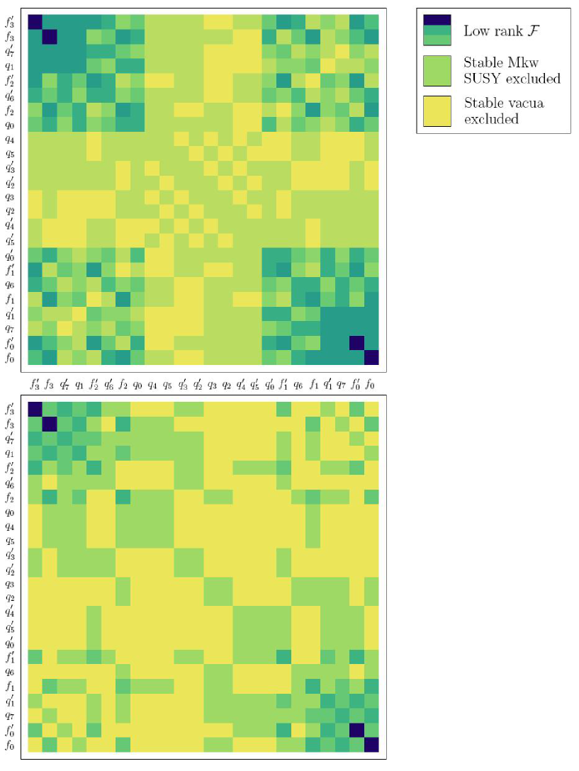
Figure 1: The rank of $\cal F$ is represented when one or two generic electric gaugings are turned on in the ${\cal N}=4$ (upper graph) and ${\cal N}=8$ (lower graph) constraints. Yellow points are excluded for moduli stabilization because ${\rm rank}{\cal F}=\#{\rm magnetic\ fluxes}-1=23$.

• ${\cal N}=4$ deformations. In figure 1 (upper graph) we sketch rank${\cal F}$ for all possible sets of one or two $f_{+}$ generic parameters. When searching for solutions different from $f_{+}=\alpha f_{-}$, the only interesting cases are those in which (4.25) is satisfied. Already at this stage of the procedure, when only two magnetic parameters are turned on, a large part of the parameter space is discarded for moduli stabilization in any vacuum. When adding more non vanishing parameters the situation gets worse because the rank of $\cal F$ increases and gets closer to the bound (4.24). An explicit counting shows that more than $95\%$ of the parameter space falls in the exclusion region. For Minkowski vacua, the exclusion region is even larger because already when ${\rm rank}{\cal F}=\#{\rm magnetic\ fluxes}-2,$ the models are not viable for moduli fixing.

• ${\cal N}=8$ deformations. For this case, we sketch rank$\cal F$ in figure 1 (lower graph). Notice that the excluded region (when only two electric gaugings with generic values are turned on) is even much larger than in the previous case. We have not found models surviving the exclusion argument that admit fully stabilized vacua with physically acceptable values for the moduli. This might find its origin in the fact that the parent ${\cal N}=8$ theory is massless and all fields are moduli at tree-level. This should be considered as a limit, the limit of maximal constraints for these kind of models.

In summary, we have shown why it is so difficult to stabilize vacua when the constraints are imposed. The extreme limit is that in which all ${\cal N}=8$ constraints are considered in the absence of sources. When sources are added and the number of supersymmetries reduces, the possibilities for stabilizing vacua increase. In the next section we show some representative examples of SUSY vacua, in different situations.

4.2 SUSY vacua

Here we present different examples to illustrate the general results about moduli fixing, and the possibility to embed string vacua in (deformed) gauged ${\cal N}=4,8$ supergravity truncations.

We start with an analysis of Type IIB AdS vacua, restricting to the case in which only fluxes that are dual to IIA geometric, RR and NSNS fluxes are turned on. We first consider a well known example [29] arising from a controlled and consistent $D=10$ setup. Then we move to the classification of all allowed isotropic models with IIA-geometric fluxes satisfying the ${\cal N}=4,8$ constraints with branes, and exhibit some of the simplest solutions. Models involving $P$-fluxes and admitting fully stabilized vacua are also displayed. We also show how examples that can be embedded in gauged supergravity can be seen as vacua spontaneously breaking ${\cal N}=4\to 1$ and we discuss further constraints imposed by Freed-Witten (FW) anomalies [30].

We then consider Minkowski vacua. We argue that when primed fluxes are turned off, the algebraic constraints generically do not allow stable Minkowski vacua satisfying the physical constraints. Finally, we display some examples.

4.2.1 Anti de Sitter

The IIB dual of the AdS solution of [29]

Let us reconsider the model introduced in [29], T-dualized to the IIB picture. Interest in analyzing this case resides in the fact that it can be uplifted to $D=10$ as a consistent supergravity solution in the IIA picture. Additionally, it is known to stabilize some of the moduli and allows for vanishing brane charges (and therefore exact embeddings in gauged supergravity).

The model is defined by the superpotential

$$W_{AF}=e_{0}+ie_{i}U_{i}-q_{r}U_{s}U_{t}+imU_{1}U_{2}U_{3}+ih_{0}S-a_{i}U_{i}S-ih_{i}T_{i}-b_{ij}T_{j}U_{i}\,,$$ (4.26)

where the following identification is chosen

$$q_{i}=-c\ ,\ \ \ \ \ e_{i}=e\ ,\ \ \ \ \ \ \ a_{i}=a\,,\ \ \ \ \ \ \ -b_{ii}=b_{ji}=b_{i}\,.$$ (4.27)

The tadpole cancelation conditions required by string theory are given by

$$N_{D7i}=\frac{1}{2}\left(mh_{i}+b_{i}c\right)\ ,\ \ \ \ \ N_{D3/O3}=\frac{1}{2}\left(h_{0}m-3ac\right)$$ (4.28)

and all other constraints are automatically satisfied. The first constraints define the charge of D7-branes wrapping the 4-cycles $\tilde{\omega}_{i}$. If such branes were present $N_{D7i}\neq 0$, they would select a different projection from that already determined by the orientifold, and therefore, even if the orbifold were removed, SUSY would be broken to ${\cal N}<4$. This is the physical reason why $N_{D7i}=0$ is the only constraint to be imposed in order to match this model with an exact ${\cal N}=4$ truncation. Here we allow for non-vanishing $N_{D7i}$ and $N_{D3/O3}$.

This effective theory admits AdS minima provided the fluxes verify

$$3h_{k}a+h_{0}b_{k}=0\,.$$ (4.29)

The vacuum is isotropic in $U_{i}=U=u_{x}+iu_{y}$. The dilaton and the real part of the Kähler fields are given purely in terms of the complex structure moduli

$$s_{x}=\frac{2u_{x}(c-mu_{y})}{a}\ ,\ \ \ \ \ \ \ t_{ix}=\frac{3as_{x}}{b_{i}}\,.$$ (4.30)

The corresponding axions, on the other hand, are not entirely fixed, and determine massless directions given by

$$s_{y}(t_{y},u_{y}) = \frac{3ea+3c(3h_{0}-7au_{y})-3mu_{y}(3h_{0}-8au_{y})-3bt_{y}a}{3a^{2}}\,,$$ (4.31)

$$t_{y} = \frac{b_{1}t_{1y}}{b}\ =\ \frac{b_{2}t_{2y}}{b}\ =\ \frac{b_{3}t_{3y}}{b}\,.$$ (4.32)

Now only the complex structure moduli remain to be stabilized. Two situations can be distinguished

• For $m=0$, the solutions are given by

  $$u_{y}=\frac{h_{0}}{3a}\ ,\ \ \ \ \ \ u_{x}^{2}=\frac{1}{9c}\left(e_{0}-\frac{h_{0}e}{a}-\frac{h_{0}^{2}c}{3a^{2}}\right)\,.$$ (4.33)

• For $m\neq 0$, one first has to solve

  $$3h_{0}^{2}m(c-mu_{y})-a^{2}(e_{0}m+u_{y}(10mu_{y}-9c)(16mu_{y}-15c))$$

  $$\ \ \ \ \ \ \ \ +~{}ah_{0}(45c^{2}-106cmu_{y}-m(e+62mu_{y}^{2}))=0$$ (4.34)

  and replace the positive solutions into

  $$u_{x}^{2}=\frac{5(h_{0}-3au_{y})(mu_{y}-c)}{am}\,.$$ (4.35)

We now want to see if this model can be considered as a deformation of a gauged ${\cal N}=4,\ 8$ supergravity truncation. The parameters of this model automatically satisfy the constraints of the deformed ${\cal N}=4$ supergravity, and can be seen as an exact truncation of ${\cal N}=4$ supergravity if $N_{D7i}=0$, as we already explained. Concerning ${\cal N}=8$, even if we set $N_{D3/O3}=0$, there is an additional equation that is not satisfied by this solution, namely

$$ab_{i}=0\,.$$ (4.36)

One would have thought that in the absence of D3/O3 charges this theory could be regarded as a truncation of an ${\cal N}=8$ gauged supergravity. However surprisingly, the constraint (4.36) cannot be satisfied by the solution.

We would now like to follow the steps of [14] in order to conceive this solution as a spontaneous SUSY breaking ${\cal N}=4\to 1$ configuration. To achieve this, one first has to set $N_{D7i}=0$. Then, as explained, instead of truncating the non-diagonal moduli through orbifolding as described in Section 2, one considers these moduli as dynamical fields, but provides them with vanishing vacuum expectation values. As explained in Section 3, this leads to a situation in which the ${\cal N}=4$ shift matrices are exactly equal to the orbifolded ones, but in this case all the SUSY directions have to be analyzed. Since the above is an AdS solution of the truncated theory, it will give rise to a non-vanishing $A_{1}^{44}$ direction and vanishing $A_{2}^{44}$ and $A_{2a4}^{\ \ \ j}$, and therefore it corresponds to a solution of the parent ${\cal N}=4$ supergravity if $\epsilon^{1}=\epsilon^{2}=\epsilon^{3}=0$ and $\epsilon^{4}\neq 0$ are taken. Whether it breaks supersymmetry or not has to be determined by evaluating the remaning directions (3.31) of the shift matrices. In particular, we focus on $A_{2}$, for which (when $m=0$)

$$-i\frac{2}{3}e^{-K/2}A_{2}^{kk}\propto\frac{a^{2}\sqrt{b_{1}b_{2}b_{3}}}{c^{1/4}\left(a^{2}e_{0}-aeh_{0}-\frac{ch_{0}}{3}\right)}\ ,\ \ \ \ k=1,2,3\ ,\ \ \ \ \ A_{2}^{44}=0\,.$$ (4.37)

Since the null space of $A_{2}$ is 1-dimensional, supersymmetry is broken spontaneously to ${\cal N}=1$ by this vacuum.

Type IIB isotropic AdS with only IIA-geometric fluxes

Here we explore models without primed fluxes turned on, and without the following fluxes

$$h_{0}=h_{1}=q_{2}=q_{3}=q_{6}=q_{7}=p_{i}=0\,,$$ (4.38)

which turn out to be T-dual to non-geometric fluxes in IIA. The only fluxes we are left with are RR, NSNS and IIA-geometric fluxes, leading to the superpotential

$$W=-f_{3}+ih_{3}S+3iq_{1}T+3if_{2}U+3h_{2}SU+3q_{0}TU-3q_{4}TU+3q_{5}TU+3f_{1}U^{2}-if_{0}U^{3}\,.$$ (4.39)

These models are not only the simplest but also perhaps the most interesting ones because all the ingredients have a well known interpretation in $D=10$, and one could try to uplift the solutions to fully consistent and under control supergravity configurations. The equations for fluxes in ${\cal N}=4$ models deformed by branes are

$$N_{D3/O3} = N_{D3}-16=\frac{1}{2}\left[f_{0}h_{3}-3f_{1}h_{2}\right]$$ (4.40)

$$N_{D7} = \frac{1}{2}\left[f_{0}q_{1}-f_{1}(q_{0}-q_{4}+q_{5})\right]$$ (4.41)

$$0 = h_{2}(q_{4}-q_{0})=h_{2}(q_{0}+q_{5})=q_{4}^{2}+q_{0}q_{5}=q_{5}^{2}-q_{0}q_{4}$$ (4.42)

There are three independent solutions to these equations

1. $h_{2}=\frac{N_{D3/O3}q_{5}}{3N_{D7}}\ ,\ \ \ f_{0}=0\ ,\ \ \ q_{0}=q_{4}=-q_{5}\ ,\ \ \ f_{1}=\frac{-2N_{D7}}{q_{5}}$

2. $h_{3}=\frac{3f_{1}h_{2}+2N_{D3/O3}}{f_{0}}\ ,\ \ \ q_{1}=\frac{2N_{D7}+f_{1}q_{5}}{f_{0}}\ ,\ \ \ q_{0}=q_{4}=-q_{5}$

3. $h_{3}=\frac{2N_{D3/O3}}{f_{0}}\ ,\ \ \ q_{1}=\frac{2N_{D7}+f_{1}q_{0}}{f_{0}}\ ,\ \ \ h_{2}=q_{4}=q_{5}=0$

The deformed ${\cal N}=8$ constraints, which for our specific choice of fluxes read

$$0=h_{2}(q_{5}-q_{4})\,,$$ (4.43)

are only automatically satisfied by solutions 3.

Here we would like to display an example of a fully stabilized AdS vacuum with D3 and D7 branes, large volume and small coupling. It is not unique and we only intend to show that string vacua of this kind exist. For instance, solutions 2 lead in particular to the following vacuum

$$s_{x}=-\frac{2i\sqrt{f_{1}}\sqrt{f_{3}}}{3h_{2}}\ ,\ \ \ t_{x}=-\frac{2i\sqrt{f_{1}}\sqrt{f_{3}}}{q_{5}}\ ,\ \ \ u_{x}=\frac{i\sqrt{f_{3}}}{3\sqrt{f_{1}}}\,,$$ (4.44)

with vanishing axions $s_{y}=t_{y}=u_{y}=0$. The brane charges in terms of the fluxes read

$$16-N_{D3} = \left(\frac{3}{2}f_{1}+\frac{5}{2}\frac{f_{2}^{2}}{f_{3}}\right)h_{2}\,,$$ (4.45)

$$N_{D7} = -\left(\frac{1}{2}f_{1}+\frac{5}{6}\frac{f_{2}^{2}}{f_{3}}\right)q_{5}\,.$$ (4.46)

As we mentioned previously, due to the isotropic symmetry, the tadpole cancelation conditions for D7 branes wrapping the three possible four-cycles coincide. Here $N_{D7}$ indicates the charge of the D7 branes in each four-cycle. We also point out that this flux configuration does not allow to include the S-dual NS7 and I7 branes. The volume and string coupling are given by

$${\rm vol}_{6}=\left(\frac{3h_{2}}{q_{5}}\right)^{3/2}\ ,\ \ \ \ \ g_{S}=\frac{3ih_{2}}{2\sqrt{f_{1}}\sqrt{f_{3}}}$$ (4.47)

Taking for example $f_{3}=1$, $q_{5}=h_{2}=3$, $f_{2}=2$ and $f_{1}=-30$, one gets a configuration with $N_{D3}=121$, $N_{D7}=35$, ${\rm vol}_{6}\sim 5$ and $g_{S}\sim 0.8$, and positive real parts of all the moduli.

On the other hand, taking for example $f_{1}=-15$, $f_{2}=3$, $f_{3}=q_{5}=h_{2}=1$, one obtains a configuration with $N_{D3/O3}=N_{D7}=0$, ${\rm vol}_{6}\sim 5$ and $g_{S}\sim 0.4$. It is interesting that all brane charges can vanish because it signals the fact that this is a vacuum of an exact truncation of gauged ${\cal N}=4$ supergravity. Therefore, it could be conceived as an ${\cal N}=4$ minimum spontaneously breaking ${\cal N}=4\to 1$. In fact, evaluating (4.44) in the shift matrix $A_{2}$, generically yields

$$-i\frac{2}{3}e^{-K/2}A_{2}^{kk}=\frac{8f_{2}\sqrt{f_{3}}}{9\sqrt{f_{1}}}-4f_{3}+\frac{4\sqrt{f_{1}}f_{3}^{3/2}}{15f_{2}}\ ,\ \ \ \ \ \ k=1,2,3$$ (4.48)

and it is non vanishing when the solution is plugged in.

Imposing the ${\cal N}=8$ constraint (4.43) implies setting either $h_{2}$ or $q_{5}$ to zero, which is not allowed in this solution and thus it does not correspond to an ${\cal N}=8$ truncation. However, if we take vanishing fluxes $f_{1}=q_{0}=q_{4}=q_{5}=h_{2}=0$ in the solutions 2 and 3, equation (4.43) is satisfied. In this case, for instance, there is a vacuum where all moduli are fixed except for a combination of axions, namely

$$s_{x}=-\frac{2\sqrt{5f_{2}}}{3\sqrt{3f_{0}}}\frac{f_{2}}{h_{3}}\ ,\ \ \ \ t_{x}=-\frac{2\sqrt{5f_{2}}}{3\sqrt{3f_{0}}}\frac{f_{2}}{q_{1}}\ ,\ \ \ \ u_{x}=\frac{\sqrt{5f_{2}}}{\sqrt{3f_{0}}}\ ,\ \ \ \ u_{y}=0\ ,\ \ \ \ h_{3}s_{y}+3q_{1}t_{y}+f_{3}=0\,.$$

Then, assigning the values $f_{2}=-5$, $f_{0}=-1$, $q_{1}=2$ and $h_{3}=4$, one obtains a configuration with $N_{D3/O3}=-14$, $N_{D7}=-1$, ${\rm vol}_{6}\sim 3$ and $g_{S}\sim 0.4$. Given that in this vacuum the net charge of 3 and 7-sources is non vanishing, the uplifting of this configuration is expected to involve D3 and D7-branes as well as O3 and O7-planes. We then see in this particular example a generic fact of these models: when ${\cal N}=8$ constraints are imposed, many (would be) stabilized fields become massless, but one can still find vacua satisfying all other constraints.

Type IIB isotropic AdS with P-fluxes

Models involving $P$-fluxes are interesting since they have an interpretation in F-theory [13]. We have found fully stabilized AdS vacua including these fluxes. For instance, taking non vanishing fluxes $f_{2},q_{1},h_{2},h_{3},p_{0},p_{1},p_{4},p_{5}$, the ${\cal N}=4$ constraints are satisfied if $p_{0}=p_{4}=-p_{5}$. The superpotential is given by

$$W=3i(q_{1}T+f_{2}U)+S(ih_{3}+3p_{1}T+3h_{2}U+3ip_{0}TU)\,,$$ (4.49)

and it is easy to verify that all the moduli can be stabilized in this model at values satisfying the physical constraints.

4.2.2 Further constraints

It is well known that, in presence of bulk fluxes, branes could have non trivial FW anomalies [30] and, therefore, certain brane configurations are not allowed. In a Type IIB setting, with magnetized branes, Chern-Simons couplings on the worldvolume of the branes lead to the gauging of certain RR axionic scalars under D-brane $U(1)$ gauge symmetries. In [31] (see also [32, 25, 33]) it was suggested that FW constraints could be understood as the requirements needed to ensure invariance of the effective superpotential under shifts of the $U(1)$ gauged axionic scalars. Also in [13] (where only magnetized 7-branes were considered), FW anomalies were shown to arise as JI of the algebra involving both, the closed string and the open string generators associated to $U(1)$ gauge fields on the brane worldvolume. FW constraints must be taken into account when dealing with specific models involving magnetized branes [34].

Generically, the topological information of a set of $N_{a}$ D-branes is encoded in six integers $(n_{a}^{i},m_{a}^{i})$: $m_{a}^{i}$ is the number of times that the D-branes wrap the $i^{th}$ ${\rm T}^{2}$ and $n_{a}^{i}$ denotes the units of magnetic flux in that torus. This notation allows us to describe different types of branes (D9, D7, etc.) [35]. Absence of anomalies imposes restrictions on these integers.

As an example, let us revisit the model (4.39) displayed above. For a generic (non isotropic) superpotential, FW contraints read (see for instance [31])

$$-h_{0}c_{0}^{a}+h_{i}c_{i}^{a} = 0\,,$$ (4.50)

$$a_{i}c_{0}^{a}+b_{ij}c_{j}^{a} = 0\,,$$ (4.51)

which in the isotropic case reduce to

$$h_{3}c_{0}^{a}+q_{1}(c_{1}^{a}+c_{2}^{a}+c_{3}^{a}) = 0\,,$$ (4.52)

$$-h_{2}c_{0}^{a}-q_{0}c_{1}^{a}+q_{4}c_{2}^{a}-q_{5}c_{3}^{a} = 0\,,$$ (4.53)

$$-h_{2}c_{0}^{a}-q_{5}c_{1}^{a}-q_{0}c_{2}^{a}+q_{4}c_{3}^{a} = 0\,,$$ (4.54)

$$-h_{2}c_{0}^{a}+q_{4}c_{1}^{a}-q_{5}c_{2}^{a}-q_{0}c_{3}^{a} = 0\,,$$ (4.55)

with $c_{0}^{a}=m_{a}^{1}m_{a}^{2}m_{a}^{2},\,c_{1}=m_{a}^{1}n_{a}^{2}n_{a}^{2},\,c_{2}=n_{a}^{1}m_{a}^{2}n_{a}^{2},\,c_{3}=n_{a}^{1}n_{a}^{2}m_{a}^{2}$.

Using the conditions $q_{0}=q_{4}=-q_{5}$ for solutions 1 and 2 above, we easily see that $q_{0}\neq 0$ implies

$$c_{1}^{a} = c_{2}^{a}=c_{3}^{a}=c^{a}\,,$$ (4.56)

$$\frac{c_{0}^{a}}{c^{a}} = \frac{q_{0}}{h_{2}}=-\frac{3q_{1}}{h_{3}}\,,$$ (4.57)

for every stack of $N^{a}$ branes. Interestingly enough, when looking at the “intersection number” of two sets $a$ and $b$ of D-branes, namely

$$I_{ab}=\prod_{i=1}^{3}\left(n_{a}^{i}m_{b}^{i}-m_{a}^{i}n_{b}^{i}\right)\,,$$ (4.58)

we find that these strong constraints lead to $I_{ab}=0$, the spectrum being non chiral. A similar situation arises for solution 3. Here if $q_{0}\neq 0$ then all coefficients $c^{a}$ must vanish. Thus, we conclude that a chiral spectrum requires $q_{0}=0$, and in this case we have seen that some linear combination of axion fields remains unfixed.

Actually, this at first sight unpleasant result is useful. As noted in [31] (in the Type IIA picture), these axions could be helpful to eliminate anomalous $U(1)$ when looking for a chiral spectrum.

4.2.3 Minkowski

No fully stabilized isotropic Minkowski vacuum with only $F,H,Q$ and $P$ fluxes

Here we show that generically, fully stabilized Minkowski vacua cannot be achieved in the absence of primed fluxes. In [16], simple models of Minkowski vacua were found with $F,H,Q$ and $P$ fluxes, which were only constrained by JI in the presence of branes. Other restrictions such as the antisymmetric constraints were not considered, and it can be checked that those conditions can only be satisfied for non vanishing $K^{ABCD}$. Therefore, one expects the $D=10$ uplifting of those vacua to involve exotic objects [24]. In the case that we are considering, we now show that it is not possible to stabilize all moduli with non-vanishing real components in a Minkowski vacuum when only $F,H,Q$ and $P$ fluxes are present. Clearly, since a Minkowski vacuum was found in [16], the proof must involve both the constraints and the structure of the superpotential. The only three facts needed to prove our statement are:

1. One can explicitly see in figure 1 that the antisymmetric constraints $q_{2}=q_{3}=q_{4}=q_{5}=p_{2}=p_{3}=p_{4}=p_{5}=0$ must generically be imposed to find SUSY Mkw vacua.

2. The superpotential has the structure

   $$W=F(U)+H(U)S+Q(U)T+P(U)ST$$ (4.59)

   and the Minkowski SUSY equations are

   $$H(U)+P(U)T = 0$$ (4.60)

   $$Q(U)+P(U)S = 0$$ (4.61)

   $$F(U)+Q(U)T=F(U)+H(U)S = 0$$ (4.62)

   $$F^{\prime}(U)+H^{\prime}(U)S+Q^{\prime}(U)T+P^{\prime}(U)ST = 0$$ (4.63)

   Since $T,S\neq 0$, one can verify from (4.60)-(4.62) that in the vacuum either $F,H,Q$ and $P$ all vanish or are non zero. In the former case, only one equation (4.63) is left to stabilize $T$ and $S$, so there will necessarily be at least one modulus. Therefore, all terms should be non vanishing.

3. $Q(U)$ and $P(U)$ are given by

   $$Q(U)=3i(q_{1}-iq_{0}U-q_{6}U^{2}+iq_{7}U^{3})\ ,\ \ P(U)=3(p_{1}-ip_{0}U-p_{6}U^{2}+ip_{7}U^{3}).$$ (4.64)

   When only two terms of each -differing by a power of $U$- are present, and the parameters of $Q$ are proportional to those of $P$, it is impossible to stabilize the real part of some modulus away from the origin. For example in the case $q_{0}=q_{1}=p_{0}=p_{1}=0$ one can verify that when $p_{6}/q_{6}=p_{7}/q_{7}$,

   $$\partial_{T}W=Q(U)+SP(U)=\frac{3}{q_{7}}U^{2}(-q_{6}+iq_{7}U)(p_{7}S+iq_{7})=0$$ (4.65)

   and then, the real part of $S$ or $U$ is forced to vanish. This is trivially generalized to all the cases.

Combining these three facts it can readily be shown that it is impossible to fully stabilize vacua in Minkowski with all real moduli non-vanishing. In fact, when primed fluxes are set to zero, together with the fluxes of point 1, it is easy to verify that the solutions to the constraints impose that either $F,H,Q$ or $P$ vanish, or $Q$ and $P$ fall in the case mentioned in point 3.

This of course does not mean that there are no Minkowski vacua, and in fact there are plenty degenerate vacua of this type. To look for partially stabilized susy Minkowski minima, it is convenient to consider only non-primed electric gaugings. This implies, on the one hand, that the constraints (3.49) and (3.50) are automatically satisfied, and on the other, that the vacuum will necessarily be Minkowski and have a continuous degeneracy in the axion-dilaton direction. We have pointed out that due to the structure of the superpotential, in general the fields are stabilized at purely imaginary values. To overcome this difficulty, we set to zero all the terms involving an even number of fields. This ensures that all the parameters in the superpotential are real, and allows for real VEV of the Kähler and complex structure moduli. After imposing the constraints we are left with the following superpotential

$$W=3f_{2}U-f_{0}U^{3}+T(3q_{1}-3q_{3}U^{2})\,.$$ (4.66)

This model has D7-branes and vanishing $N_{D3/O3}$

$$N_{D7}=\frac{1}{2}\left[f_{0}q_{1}+f_{2}q_{3}\right]\ ,\ \ \ \ N_{D3/O3}=0\,.$$ (4.67)

In particular, for $f_{0}=3f_{2}q_{3}/q_{1}$, it admits minima with the following moduli

$$T=-\frac{f_{2}}{\sqrt{q_{1}}\sqrt{q_{3}}}\,,\ \ \ U=\frac{\sqrt{q_{1}}}{\sqrt{q_{3}}}\,,\ \ \ \forall S\,.$$ (4.68)

As we anticipated, since $W$ does not depend on $S$, its Kahler derivatives with respect to $S$ are proportional to the superpotential itself, so every SUSY vacua is necessarily Minkowski. Let us finally point out that this solution can lie in the large volume and small coupling regimes by suitable choices of the parameters, and consistency of the solution requires non vanishing $N_{D7}$.

5 Summary and outlook.

Compactifications of string theory to $D=4$ can preserve different amounts of supersymmetries. The paradigm of low scale physics has been to construct ${\cal N}=1$ effective theories in which supersymmetry is spontaneously or dynamically broken at low energies. This can be realized in compactifications on Calabi-Yau manifolds, or alternatively on spaces with reduced holonomy in which the large supersymmertic structure is explicitly broken by projections. In this case, the effective theory is a truncation of the parent theory, and one expects that it inherits many of the original characteristic features.

In this work we have focused on Type IIB toroidal compactifications in which supersymmetry is broken from ${\cal N}=8$ to ${\cal N}=4$ by an orientifold projection incorporating O3 planes. In addition, supersymmetry is further broken to ${\cal N}=1$ by a $\mathbb{Z}_{2}\times\mathbb{Z}_{2}$ orbifold projection, where the structure group is enhanced to $SU(3)$ at the fixed points. The untwisted sector of the resulting theory is given by direct truncation of the parent ${\cal N}=4$ theory, so it is expected to match some ${\cal N}=4$ gauged supergravity truncation. We have clarified the connection between these string orbifolds and gauged supergravity truncations.

We established the full dictionary between the scalar sector of gauged supergravity and the moduli space of the string orbifold (3.18) and, by extending the results of [13], we determined the complete connection between fluxes and gaugings (3.22). Then, we analyzed the SUSY variations of the fermions in gauged supergravity, which are parameterized by the so-called shift matrices (3.12). These matrices fix the structure of the scalar potential (3.4) and the amount of supersymmetry preserved by the vacuum (3.25). We applied the orbifold projection on the shift matrices and recovered the effective Type IIB superpotential (2.14) and the scalar potential obtained from it. This complements the results of [13], where the complete set of constraints on fluxes in the string side were shown to exactly match the gauged supergravity consistency conditions for gaugings (3.8).

We have extended the analysis so as to include branes in this setup. A brief computation shows that when these sources are present, the structure of the effective scalar potential remains unaltered in the untwisted sector. However, branes source the tadpole cancelation conditions of string theory, and in many cases break the exact matching with the quadratic constraints of gauged supergravity. Such is the case of D7 branes, which project out a different combination of gravitini than the orientifold planes and break ${\cal N}=4$ explicitly. Therefore, even if the effective theory looks like a gauged supergravity truncation in the presence of branes, strictly speaking it is not. Rather, it is a deformation that corresponds to an exact truncation when no SUSY-breaking sources are present.

We have also obtained additional constraints on fluxes by comparing the scalar potentials of gauged ${\cal N}=4$ and ${\cal N}=8$ supergravities (3.49)-(3.50). Such constraints include the tadpole cancelation condition stating that no D3/O3 sources or any of their duals should be present. From a $D=4$ perspective, such constraints seem to correspond to a cancelation of the scalar masses required by ${\cal N}=8$ consistency.

Having collected the full set of constraints that one expects in these string truncations, we addressed the problem of moduli fixing. The rich structure of the superpotential (2.14) is highly constrained by the consistency requirements. We have seen that in most models the constraints force a proportionality between electric and magnetic gaugings, and showed that it is not possible to stabilize all moduli in such case. With this argument, we were able to exclude large regions of the parameter space and focus on models which have potentiality for full moduli fixing. We displayed some examples of AdS and Minkowski SUSY vacua, analyzed their ${\cal N}=4,8$ origin, and also discussed the possibility that they spontaneously break ${\cal N}=4\to 1$. Some of the examples have all moduli stabilized in a vacuum with (or without) branes in large compactification volume and small coupling regimes. In a subset of AdS vacua, we have explicitly shown that, as observed in [31], a chiral spectrum is connected with the presence of unfixed axions.

Note added: Soon after this paper appeared in the arXiv, we received the preprint [37], having some overlap with parts of our work. See also the more recent paper [38].

Acknowledgments We thank E. Andrés, G. Dall’Agata, G. A. Guarino and H. Samtleben for useful discussions, comments and correspondence, and especially P. Cámara and M. Graña, for also suggesting important improvements on the manuscript. We are grateful to D. Mitnik for providing access to his computer network. This work was partially supported by MINCYT (Ministerio de Ciencia, Tecnología e Innovación Productiva of Argentina) and ECOS-Sud France binational collaboration project A08E06. D.M. benefited from the CNOUS/CONICET Bernardo Houssay Fellowship and ANR grant 08 JCJC 0001 0.

Appendix A Constraints and superpotential.

Here we would like to compile the explicit form of the constraints and superpotential, and link the different notations used for the fluxes and the parameters.

The gauge algebra has the form

$\ \ \;\;\left[X^{a},X^{b}\right]\ \ =\ \ -\tilde{F}^{abp}Z_{p}+Q^{ab}_{p}X^{p}$		$\ \ \ \;\left[\bar{X}^{a},\bar{X}^{b}\right]\ \ =\ \ -\tilde{H}^{abp}\bar{Z}_{p}+P^{ab}_{p}\bar{X}^{p}$
$\left[X^{a},Z_{b}\right]\ \ =\ \ Q^{\prime a}_{bp}X^{p}-Q^{ap}_{b}Z_{p}$		$\left[\bar{X}^{a},\bar{Z}_{b}\right]\ \ =\ \ P_{bp}^{\prime a}\bar{X}^{p}-P^{ap}_{b}\bar{Z}_{p}$
$\ \ \left[Z_{a},Z_{b}\right]\ \ =\ \ -F_{abp}^{\prime}X^{p}+Q_{ab}^{\prime p}Z_{p}$		$\ \ \;\left[\bar{Z}_{a},\bar{Z}_{b}\right]\ \ =\ \ -H_{abp}^{\prime}\bar{X}^{p}+P_{ab}^{\prime p}\bar{Z}_{p}$

$$\left[X^{a},\bar{X}^{b}\right]\ \ =\ \ Q^{ab}_{p}\bar{X}^{p}-\tilde{F}^{abp}\bar{Z}_{p}\ \ =\ \ P_{p}^{ab}X^{p}-\tilde{H}^{abp}Z_{p}$$

$$\left[\bar{X}^{a},Z_{b}\right] = \left[X^{a},\bar{Z}_{b}\right]\ \ =\ \ Q^{\prime a}_{bp}\bar{X}^{p}-Q^{ap}_{b}\bar{Z}_{p}\ \ =\ \ P^{\prime a}_{bp}X^{p}-P^{ap}_{b}Z_{p}$$ (A.1)

$$\left[Z_{a},\bar{Z}_{b}\right]\ \ =\ \ -F^{\prime}_{abp}\bar{X}^{p}+Q^{\prime p}_{ab}\bar{Z}_{p}\ \ =\ \ P^{\prime p}_{ab}Z_{p}-H^{\prime}_{abp}X^{p}\,$$

The last equalities are enforced to ensure antisymmetry of the commutators, and imply the following “antisymmetry constraints” for fluxes (3.8)

$$Q_{ab}^{\prime p}P_{cp}^{\prime l}-P_{ab}^{\prime p}Q_{cp}^{\prime l}+F^{\prime}_{pab}P^{lp}_{c}-H^{\prime}_{pab}Q^{lp}_{c} = 0$$

$$P_{ab}^{\prime p}F_{clp}^{\prime}-Q_{ab}^{\prime p}H^{\prime}_{clp}-F^{\prime}_{pab}P_{cl}^{\prime p}+H^{\prime}_{pab}Q^{\prime p}_{cl} = 0$$

$$Q_{ab}^{\prime p}P_{p}^{cl}-P_{ab}^{\prime p}Q_{p}^{cl}+F^{\prime}_{pab}\tilde{H}^{clp}-H^{\prime}_{pab}\tilde{F}^{clp} = 0$$

$$Q^{pb}_{a}P_{cp}^{\prime l}-P_{a}^{pb}Q_{cp}^{\prime l}+Q^{\prime b}_{pa}P^{lp}_{c}-P^{\prime b}_{pa}Q^{lp}_{c} = 0$$

$$Q^{pb}_{a}P^{cl}_{p}-P^{pb}_{a}Q_{p}^{cl}+Q^{\prime b}_{pa}\tilde{H}^{clp}-P^{\prime b}_{pa}\tilde{F}^{clp} = 0$$

$$\tilde{F}^{pab}P^{cl}_{p}-\tilde{H}^{pab}Q_{p}^{cl}+Q^{ab}_{p}\tilde{H}^{clp}-P^{ab}_{p}\tilde{F}^{clp} = 0$$ (A.2)

Using these equations, the Jacobi identities for the full set of fluxes can be written as

$Q_{[ab}^{\prime p}Q_{c]p}^{\prime l}+F^{\prime}_{p[ab}Q^{lp}_{c]}\ \ =\ \ 0$		$Q_{[ab}^{\prime p}F_{c]lp}^{\prime}+F^{\prime}_{p[ab}Q_{c]l}^{\prime p}\ \ =\ \ 0$
$Q_{[ab}^{\prime p}P_{c]p}^{\prime l}+F^{\prime}_{p[ab}P^{lp}_{c]}\ \ =\ \ 0$		$Q_{[ab}^{\prime p}H_{c]lp}^{\prime}+F^{\prime}_{p[ab}P_{c]l}^{\prime p}\ \ =\ \ 0$
$P_{[ab}^{\prime p}P_{c]p}^{\prime l}+H^{\prime}_{p[ab}P^{lp}_{c]}\ \ =\ \ 0$		$P_{[ab}^{\prime p}H_{c]lp}^{\prime}+H^{\prime}_{p[ab}P_{c]l}^{\prime p}\ \ =\ \ 0$

$$F_{pab}^{\prime}\tilde{F}^{clp}+Q_{ab}^{\prime p}Q^{cl}_{p}-Q^{pc}_{[a}Q_{b]p}^{\prime l}-Q_{p[a}^{\prime c}Q_{b]}^{lp} = 0$$

$$F_{pab}^{\prime}\tilde{H}^{clp}+Q_{ab}^{\prime p}P^{cl}_{p}-Q^{pc}_{[a}P_{b]p}^{\prime l}-Q_{p[a}^{\prime c}P_{b]}^{lp} = 0$$ (A.3)

$$H_{pab}^{\prime}\tilde{H}^{clp}+P_{ab}^{\prime p}P^{cl}_{p}-P^{pc}_{[a}P_{b]p}^{\prime l}-P_{p[a}^{\prime c}P_{b]}^{lp} = 0$$

$Q_{p}^{[bc}Q^{l]p}_{a}-Q_{pa}^{\prime[b}\tilde{F}^{cl]p}\ \ =\ \ 0$		$\tilde{F}^{p[ab}Q^{c]l}_{p}+Q^{[ab}_{p}\tilde{F}^{c]lp}\ \ =\ \ 0$
$P^{[bc}_{p}Q^{l]p}_{a}-Q_{pa}^{\prime[b}\tilde{H}^{cl]p}\ \ =\ \ 0$		$\tilde{F}^{p[ab}P^{c]l}_{p}+Q^{[ab}_{p}\tilde{H}^{c]lp}\ \ =\ \ 0$
$P_{p}^{[bc}P^{l]p}_{a}-P_{pa}^{\prime[b}\tilde{H}^{cl]p}\ \ =\ \ 0$		$\tilde{H}^{p[ab}P^{c]l}_{p}+P^{[ab}_{p}\tilde{H}^{c]lp}\ \ =\ \ 0$

The superpotential explicitly reads

$$W = e_{0}-i\sum_{i=1}^{3}h_{i}T_{i}+\frac{1}{2}\sum_{l\not=m\not=n}h^{\prime}_{l}T_{m}T_{n}+ie^{\prime}_{0}T_{1}T_{2}T_{3}$$ (A.4)

$$+ \bigg{(}ih_{0}-\sum_{i=1}^{3}f_{i}T_{i}-\frac{i}{2}\sum_{l\not=m\not=n}f^{\prime}_{l}T_{m}T_{n}-h^{\prime}_{0}T_{1}T_{2}T_{3}\bigg{)}S$$

$$+ \sum_{i=1}^{3}\left[\bigg{(}-a_{i}+i\sum_{j=1}^{3}g_{ij}T_{j}-\frac{1}{2}\sum_{l\not=m\not=n}g^{\prime}_{il}T_{m}T_{n}+ia^{\prime}_{i}T_{1}T_{2}T_{3}\bigg{)}S\right.$$

$$+ \left.ie_{i}-\sum_{j=1}^{3}b_{ij}T_{j}-\frac{i}{2}\sum_{l\not=m\not=n}b^{\prime}_{il}T_{m}T_{n}-e^{\prime}_{i}T_{1}T_{2}T_{3}\right]U_{i}$$

$$+ \frac{1}{2}\sum_{r\not=s\not=t}\left[\bigg{(}i\bar{a}_{r}+\sum_{j=1}^{3}\bar{g}_{rj}T_{j}+\frac{i}{2}\sum_{l\not=m\not=n}\bar{g}^{\prime}_{rl}T_{m}T_{n}-\bar{a}^{\prime}_{r}T_{1}T_{2}T_{3}\bigg{)}S\right.$$

$$- \left.q_{r}+i\sum_{j=1}^{3}\bar{b}_{rj}T_{j}-\frac{1}{2}\sum_{l\not=m\not=n}\bar{b}^{\prime}_{rl}T_{m}T_{n}+iq^{\prime}_{r}T_{1}T_{2}T_{3}\right]U_{s}U_{t}$$

$$+ \left[-\bigg{(}\bar{h}_{0}+i\sum_{j=1}^{3}\bar{f}_{j}T_{j}-\frac{1}{2}\sum_{l\not=m\not=n}\bar{f}^{\prime}_{l}T_{m}T_{n}+i\bar{h}^{\prime}_{0}T_{1}T_{2}T_{3}\bigg{)}S\right.$$

$$+ \left.im+\sum_{j=1}^{3}\bar{h}_{j}T_{j}+\frac{i}{2}\sum_{l\not=m\not=n}\bar{h}^{\prime}_{l}T_{m}T_{n}-m^{\prime}T_{1}T_{2}T_{3}\right]U_{1}U_{2}U_{3}\,.$$

The connection between these parameters and the IIB fluxes can be read from Table 1. We also refer to the original literature [16, 13] for additional details on the notation, in particular for links with IIA and Type I fluxes.

Finally, we display the ${\cal N}=8$ constraints (for simplicity when only $F,H,Q$ and $P$ fluxes are turned on)

$$\tilde{F}^{pqr}H_{pqr}=0\ ,\ \ \ \ H_{pqa}Q^{pq}_{b}-F_{pqa}P^{pq}_{b}=0\ ,\ \ \ \ \hat{\sigma}_{pq}P^{p[a}_{[c}Q^{b]q}_{d]}=0\ ,\ \ \ \ \hat{\sigma}=i\sigma^{2}\otimes 1_{3}$$ (A.5)

Appendix B Useful formulas.

Vector indices of $SU(4)$ are raised and lowered with complex conjugation, as $v_{i}=(v^{i})^{*}$. On the other hand, $SO(6)$ vectors can be conveniently described through antisymmetric tensors $\nu^{ij}$ subject to the pseudo-reality constraint

$$\nu_{ij}=(\nu^{ij})^{*}=\frac{1}{2}\epsilon_{ijkl}\nu^{kl}\,,$$ (B.1)

with scalar product

$$\nu_{m}\nu_{m}=\frac{1}{2}\epsilon_{ijkl}\nu^{ij}\nu^{kl}\,.$$ (B.2)

Being $\{e^{1},\dots,e^{6}\}$ the canonical basis of $SO(6)$, then the corresponding basis of $SU(4)$ is given by

$$e^{1}\leftrightarrow(\gamma^{1})^{ij}=\frac{i}{2}\sigma^{2}\otimes\sigma^{1}\ ,\ \ \ \ e^{2}\leftrightarrow(\gamma^{2})^{ij}=-\frac{i}{2}\sigma^{2}\otimes\sigma^{3}\ ,\ \ \ \ e^{3}\leftrightarrow(\gamma^{3})^{ij}=\frac{i}{2}1\otimes\sigma^{2}\,,$$

$$e^{4}\leftrightarrow(\gamma^{4})^{ij}=-\frac{1}{2}\sigma^{1}\otimes\sigma^{2}\ ,\ \ \ \ e^{5}\leftrightarrow(\gamma^{5})^{ij}=-\frac{1}{2}\sigma^{1}\otimes 1\ ,\ \ \ \ e^{6}\leftrightarrow(\gamma^{6})^{ij}=\frac{1}{2}\sigma^{3}\otimes\sigma^{2}\,.$$

And we can rewrite the coset representative as

$$\nu^{M}=\nu_{m}^{\quad M}e^{m}\leftrightarrow\nu_{m}^{\quad M}(\gamma^{m})^{ij}\,.$$ (B.3)

Also the basis matrices have the following useful properties

$${\rm Tr}[\gamma_{i_{1}}\gamma^{*}_{i_{2}}\gamma_{i_{3}}\gamma^{*}_{i_{4}}] = \frac{1}{4}(\delta_{i_{1}i_{2}}\delta_{i_{3}i_{4}}-\delta_{i_{1}i_{3}}\delta_{i_{2}i_{4}}+\delta_{i_{1}i_{4}}\delta_{i_{2}i_{3}})\,,$$ (B.4)

$${\rm Tr}[\gamma_{i_{1}}^{*}\gamma_{i_{2}}\gamma_{i_{3}}^{*}\gamma_{i_{4}}\gamma_{i_{5}}^{*}\gamma_{i_{6}}] = -\frac{i}{16}\epsilon_{i_{1}i_{2}i_{3}i_{4}i_{5}i_{6}}-\frac{1}{16}[\delta_{i_{1}i_{2}}\delta_{i_{3}i_{4}}\delta_{i_{5}i_{6}}-\delta_{i_{1}i_{2}}\delta_{i_{3}i_{5}}\delta_{i_{4}i_{6}}+\delta_{i_{1}i_{2}}\delta_{i_{3}i_{6}}\delta_{i_{4}i_{5}}-$$

$$\ \ \ \ \ \ \ \ \ \ \ \ \ \ \ \ \ \ \ \ \ \ \ \ \ \ \ \delta_{i_{1}i_{5}}\delta_{i_{3}i_{4}}\delta_{i_{2}i_{6}}+\delta_{i_{1}i_{6}}\delta_{i_{3}i_{4}}\delta_{i_{2}i_{5}}-\delta_{i_{1}i_{3}}\delta_{i_{2}i_{4}}\delta_{i_{5}i_{6}}+$$

$$\ \ \ \ \ \ \ \ \ \ \ \ \ \ \ \ \ \ \ \ \ \ \ \ \ \ \ \delta_{i_{1}i_{4}}\delta_{i_{2}i_{3}}\delta_{i_{5}i_{6}}+\delta_{i_{1}i_{3}}\delta_{i_{2}i_{5}}\delta_{i_{4}i_{6}}-\delta_{i_{1}i_{3}}\delta_{i_{2}i_{6}}\delta_{i_{4}i_{5}}-$$

$$\ \ \ \ \ \ \ \ \ \ \ \ \ \ \ \ \ \ \ \ \ \ \ \ \ \ \ \delta_{i_{1}i_{5}}\delta_{i_{2}i_{3}}\delta_{i_{4}i_{6}}+\delta_{i_{1}i_{6}}\delta_{i_{2}i_{3}}\delta_{i_{4}i_{5}}-\delta_{i_{1}i_{4}}\delta_{i_{2}i_{5}}\delta_{i_{3}i_{6}}+$$

$$\ \ \ \ \ \ \ \ \ \ \ \ \ \ \ \ \ \ \ \ \ \ \ \ \ \ \ \delta_{i_{1}i_{4}}\delta_{i_{2}i_{6}}\delta_{i_{3}i_{5}}+\delta_{i_{1}i_{5}}\delta_{i_{2}i_{4}}\delta_{i_{3}i_{6}}-\delta_{i_{1}i_{6}}\delta_{i_{2}i_{4}}\delta_{i_{3}i_{5}}]\,,$$

that allow to link the expressions (3.4) and (3.13) of the scalar potentials.

Table 1: Dictionary between the different notations adopted for the flux parameters.

$F$	param	$\mathbb{Z}_{3}$	$H$	param	$\mathbb{Z}_{3}$	$F^{\prime}$	param	$\mathbb{Z}_{3}$	$H^{\prime}$	param	$\mathbb{Z}_{3}$
$F_{123}=-\tilde{F}^{456}$	$-m$	$f_{0}$	$H_{123}$	$\ \ \bar{h}_{0}$	$h_{0}$	$F^{\prime}_{123}$	$\ \ m^{\prime}$	$f^{\prime}_{0}$	$H_{123}^{\prime}$	$-\bar{h}_{0}^{\prime}$	$h^{\prime}_{0}$
$F_{423}=\tilde{F}^{156}$	$-q_{1}$	$f_{1}$	$H_{423}$	$-\bar{a}_{1}$	$h_{1}$	$F^{\prime}_{423}$	$-q_{1}^{\prime}$	$f^{\prime}_{1}$	$H_{423}^{\prime}$	$\ \ \bar{a}_{1}^{\prime}$	$h^{\prime}_{1}$
$F_{153}=\tilde{F}^{426}$	$-q_{2}$	$f_{1}$	$H_{153}$	$-\bar{a}_{2}$	$h_{1}$	$F^{\prime}_{153}$	$-q_{2}^{\prime}$	$f^{\prime}_{1}$	$H_{153}^{\prime}$	$\ \ \bar{a}_{2}^{\prime}$	$h^{\prime}_{1}$
$F_{126}=\tilde{F}^{453}$	$-q_{3}$	$f_{1}$	$H_{126}$	$-\bar{a}_{3}$	$h_{1}$	$F^{\prime}_{126}$	$-q_{3}^{\prime}$	$f^{\prime}_{1}$	$H_{126}^{\prime}$	$\ \ \bar{a}_{3}^{\prime}$	$h^{\prime}_{1}$
$F_{156}=-\tilde{F}^{423}$	$\ \ e_{1}$	$f_{2}$	$H_{156}$	$-a_{1}$	$h_{2}$	$F^{\prime}_{156}$	$-e_{1}^{\prime}$	$f^{\prime}_{2}$	$H_{156}^{\prime}$	$-a_{1}^{\prime}$	$h^{\prime}_{2}$
$F_{426}=-\tilde{F}^{153}$	$\ \ e_{2}$	$f_{2}$	$H_{426}$	$-a_{2}$	$h_{2}$	$F^{\prime}_{426}$	$-e_{2}^{\prime}$	$f^{\prime}_{2}$	$H_{426}^{\prime}$	$-a_{2}^{\prime}$	$h^{\prime}_{2}$
$F_{453}=-\tilde{F}^{126}$	$\ \ e_{3}$	$f_{2}$	$H_{453}$	$-a_{3}$	$h_{2}$	$F^{\prime}_{453}$	$-e_{3}^{\prime}$	$f^{\prime}_{2}$	$H_{453}^{\prime}$	$-a_{3}^{\prime}$	$h^{\prime}_{2}$
$F_{456}=\tilde{F}^{123}$	$-e_{0}$	$f_{3}$	$H_{456}$	$\ \ h_{0}$	$h_{3}$	$F^{\prime}_{456}$	$\ \ e_{0}^{\prime}$	$f^{\prime}_{3}$	$H_{456}^{\prime}$	$-h_{0}^{\prime}$	$h^{\prime}_{3}$

$Q$	param	$\mathbb{Z}_{3}$
$\left(\begin{array}[]{ccc}\!\!\!Q^{23}_{4}&Q^{31}_{5}&Q^{12}_{6}\!\!\!\end{array}\right)$	$-\left(\begin{array}[]{ccc}\!\!\!h_{1}&h_{2}&h_{3}\!\!\!\end{array}\right)$	$q_{1}$
$\left(\begin{array}[]{ccc}\!\!\!-Q^{23}_{1}&\,Q^{34}_{5}&\,Q^{42}_{6}\\ \,Q^{53}_{4}&\!\!\!-Q^{31}_{2}&\,Q^{15}_{6}\\ \,Q^{26}_{4}&\,Q^{61}_{5}&\!\!\!-Q^{12}_{3}\end{array}\right)$	$\left(\begin{array}[]{ccc}b_{11}&b_{12}&b_{13}\\ b_{21}&b_{22}&b_{23}\\ b_{31}&b_{32}&b_{33}\end{array}\right)$	$\begin{matrix}b_{ii}=-q_{0}\\ b_{12}=b_{23}=b_{31}=q_{4}\\ b_{13}=b_{21}=b_{32}=-q_{5}\end{matrix}$
$\left(\begin{array}[]{ccc}\!\!\!Q^{56}_{1}&Q^{64}_{2}&Q^{45}_{3}\!\!\!\end{array}\right)$	$\!\!-\left(\begin{array}[]{ccc}\!\!\!\bar{h}_{1}&\bar{h}_{2}&\bar{h}_{3}\!\!\!\end{array}\right)$	$q_{7}$
$\left(\begin{array}[]{ccc}\!\!\!-Q^{56}_{4}&\,Q^{61}_{2}&\,Q^{15}_{3}\\ \,Q^{26}_{1}&\!\!\!-Q^{64}_{5}&\,Q^{42}_{3}\\ \,Q^{53}_{1}&\,Q^{34}_{2}&\!\!\!-Q^{45}_{6}\end{array}\right)$	$\left(\begin{array}[]{ccc}\bar{b}_{11}&\bar{b}_{12}&\bar{b}_{13}\\ \bar{b}_{21}&\bar{b}_{22}&\bar{b}_{23}\\ \bar{b}_{31}&\bar{b}_{32}&\bar{b}_{33}\end{array}\right)$	$\begin{matrix}\bar{b}_{ii}=-q_{6}\\ \bar{b}_{12}=\bar{b}_{23}=\bar{b}_{31}=-q_{3}\\ \bar{b}_{13}=\bar{b}_{21}=\bar{b}_{32}=q_{2}\end{matrix}$

$Q^{\prime}$	param	$\mathbb{Z}_{3}$
$\left(\begin{array}[]{ccc}\!\!\!Q_{56}^{\prime 1}&Q_{64}^{\prime 2}&Q_{45}^{\prime 3}\!\!\!\end{array}\right)$	$-\left(\begin{array}[]{ccc}\!\!\!h_{1}^{\prime}&h_{2}^{\prime}&h_{3}^{\prime}\!\!\!\end{array}\right)$	$q^{\prime}_{7}$
$\left(\begin{array}[]{ccc}\!\!\!-Q_{65}^{\prime 4}&\,Q_{16}^{\prime 2}&\,Q_{51}^{\prime 3}\\ \,Q_{62}^{\prime 1}&\!\!\!-Q_{46}^{\prime 5}&\,Q_{24}^{\prime 3}\\ \,Q_{35}^{\prime 1}&\,Q_{43}^{\prime 2}&\!\!\!-Q_{54}^{\prime 6}\end{array}\right)$	$\left(\begin{array}[]{ccc}b_{11}^{\prime}&b_{12}^{\prime}&b_{13}^{\prime}\\ b_{21}^{\prime}&b_{22}^{\prime}&b_{23}^{\prime}\\ b_{31}^{\prime}&b_{32}^{\prime}&b_{33}^{\prime}\end{array}\right)$	$\begin{matrix}b^{\prime}_{ii}=\ \ q^{\prime}_{6}\\ b^{\prime}_{12}=b^{\prime}_{23}=b^{\prime}_{31}=q^{\prime}_{3}\\ b^{\prime}_{13}=b^{\prime}_{21}=b^{\prime}_{32}=-q^{\prime}_{2}\end{matrix}$
$\left(\begin{array}[]{ccc}\!\!\!Q_{32}^{\prime 4}&Q_{13}^{\prime 5}&Q_{21}^{\prime 6}\!\!\!\end{array}\right)$	$\!\!-\left(\begin{array}[]{ccc}\!\!\!\bar{h}_{1}^{\prime}&\bar{h}_{2}^{\prime}&\bar{h}_{3}^{\prime}\!\!\!\end{array}\right)$	$-q^{\prime}_{1}$
$\left(\begin{array}[]{ccc}\!\!\!-Q_{23}^{\prime 1}&\,Q_{34}^{\prime 5}&\,Q_{42}^{\prime 6}\\ \,Q_{53}^{\prime 4}&\!\!\!-Q_{31}^{\prime 2}&\,Q_{15}^{\prime 6}\\ \,Q_{26}^{\prime 4}&\,Q_{61}^{\prime 5}&\!\!\!-Q_{12}^{\prime 3}\end{array}\right)$	$\left(\begin{array}[]{ccc}\bar{b}_{11}^{\prime}&\bar{b}_{12}^{\prime}&\bar{b}_{13}^{\prime}\\ \bar{b}_{21}^{\prime}&\bar{b}_{22}^{\prime}&\bar{b}_{23}^{\prime}\\ \bar{b}_{31}^{\prime}&\bar{b}_{32}^{\prime}&\bar{b}_{33}^{\prime}\end{array}\right)$	$\begin{matrix}\bar{b}^{\prime}_{ii}=-q^{\prime}_{0}\\ \bar{b}^{\prime}_{12}=\bar{b}^{\prime}_{23}=\bar{b}^{\prime}_{31}=q^{\prime}_{4}\\ \bar{b}^{\prime}_{13}=\bar{b}^{\prime}_{21}=\bar{b}^{\prime}_{32}=-q^{\prime}_{5}\end{matrix}$

$P$	param	${\mathbb{Z}}_{3}$
$\left(\begin{array}[]{ccc}\!\!\!P^{23}_{4}&P^{31}_{5}&P^{12}_{6}\!\!\!\end{array}\right)$	$-\left(\begin{array}[]{ccc}\!\!\!f_{1}&f_{2}&f_{3}\!\!\!\end{array}\right)$	$p_{1}$
$\left(\begin{array}[]{ccc}\!\!\!-P^{23}_{1}&\,P^{34}_{5}&\,P^{42}_{6}\\ \,P^{53}_{4}&\!\!\!-P^{31}_{2}&\,P^{15}_{6}\\ \,P^{26}_{4}&\,P^{61}_{5}&\!\!\!-P^{12}_{3}\end{array}\right)$	$\left(\begin{array}[]{ccc}g_{11}&g_{12}&g_{13}\\ g_{21}&g_{22}&g_{23}\\ g_{31}&g_{32}&g_{33}\end{array}\right)$	$\begin{matrix}g_{ii}=-p_{0}\\ g_{12}=g_{23}=g_{31}=p_{4}\\ g_{13}=g_{21}=g_{32}=-p_{5}\end{matrix}$
$\left(\begin{array}[]{ccc}\!\!\!P^{56}_{1}&P^{64}_{2}&P^{45}_{3}\!\!\!\end{array}\right)$	$\!\!-\left(\begin{array}[]{ccc}\!\!\!\bar{f}_{1}&\bar{f}_{2}&\bar{f}_{3}\!\!\!\end{array}\right)$	$p_{7}$
$\left(\begin{array}[]{ccc}\!\!\!-P^{56}_{4}&\,P^{61}_{2}&\,P^{15}_{3}\\ \,P^{26}_{1}&\!\!\!-P^{64}_{5}&\,P^{42}_{3}\\ \,P^{53}_{1}&\,P^{34}_{2}&\!\!\!-P^{45}_{6}\end{array}\right)$	$\left(\begin{array}[]{ccc}\bar{g}_{11}&\bar{g}_{12}&\bar{g}_{13}\\ \bar{g}_{21}&\bar{g}_{22}&\bar{g}_{23}\\ \bar{g}_{31}&\bar{g}_{32}&\bar{g}_{33}\end{array}\right)$	$\begin{matrix}\bar{g}_{ii}=-p_{6}\\ \bar{g}_{12}=\bar{g}_{23}=\bar{g}_{31}=-p_{3}\\ \bar{g}_{13}=\bar{g}_{21}=\bar{g}_{32}=p_{2}\end{matrix}$

$P^{\prime}$	param	${\mathbb{Z}}_{3}$
$\left(\begin{array}[]{ccc}\!\!\!P_{56}^{\prime 1}&P_{64}^{\prime 2}&P_{45}^{\prime 3}\!\!\!\end{array}\right)$	$-\left(\begin{array}[]{ccc}\!\!\!f_{1}^{\prime}&f_{2}^{\prime}&f_{3}^{\prime}\!\!\!\end{array}\right)$	$p^{\prime}_{7}$
$\left(\begin{array}[]{ccc}\!\!\!-P_{65}^{\prime 4}&\,P_{16}^{\prime 2}&\,P_{51}^{\prime 3}\\ \,P_{62}^{\prime 1}&\!\!\!-P_{46}^{\prime 5}&\,P_{24}^{\prime 3}\\ \,P_{35}^{\prime 1}&\,P_{43}^{\prime 2}&\!\!\!-P_{54}^{\prime 6}\end{array}\right)$	$\left(\begin{array}[]{ccc}g_{11}^{\prime}&g_{12}^{\prime}&g_{13}^{\prime}\\ g_{21}^{\prime}&g_{22}^{\prime}&g_{23}^{\prime}\\ g_{31}^{\prime}&g_{32}^{\prime}&g_{33}^{\prime}\end{array}\right)$	$\begin{matrix}g^{\prime}_{ii}=p^{\prime}_{6}\\ g^{\prime}_{12}=g^{\prime}_{23}=g^{\prime}_{31}=p^{\prime}_{3}\\ g^{\prime}_{13}=g^{\prime}_{21}=g^{\prime}_{32}=-p^{\prime}_{2}\end{matrix}$
$\left(\begin{array}[]{ccc}\!\!\!P_{32}^{\prime 4}&P_{13}^{\prime 5}&P_{21}^{\prime 6}\!\!\!\end{array}\right)$	$\!\!-\left(\begin{array}[]{ccc}\!\!\!\bar{f}_{1}^{\prime}&\bar{f}_{2}^{\prime}&\bar{f}_{3}^{\prime}\!\!\!\end{array}\right)$	$-p^{\prime}_{1}$
$\left(\begin{array}[]{ccc}\!\!\!-P_{23}^{\prime 1}&\,P_{34}^{\prime 5}&\,P_{42}^{\prime 6}\\ \,P_{53}^{\prime 4}&\!\!\!-P_{31}^{\prime 2}&\,P_{15}^{\prime 6}\\ \,P_{26}^{\prime 4}&\,P_{61}^{\prime 5}&\!\!\!-P_{12}^{\prime 3}\end{array}\right)$	$\left(\begin{array}[]{ccc}\bar{g}_{11}^{\prime}&\bar{g}_{12}^{\prime}&\bar{g}_{13}^{\prime}\\ \bar{g}_{21}^{\prime}&\bar{g}_{22}^{\prime}&\bar{g}_{23}^{\prime}\\ \bar{g}_{31}^{\prime}&\bar{g}_{32}^{\prime}&\bar{g}_{33}^{\prime}\end{array}\right)$	$\begin{matrix}\bar{g}^{\prime}_{ii}=-p^{\prime}_{0}\\ \bar{g}^{\prime}_{12}=\bar{g}^{\prime}_{23}=\bar{g}^{\prime}_{31}=p^{\prime}_{4}\\ \bar{g}^{\prime}_{13}=\bar{g}^{\prime}_{21}=\bar{g}^{\prime}_{32}=-p^{\prime}_{5}\end{matrix}$

References

- [1] M. Grana, “Flux compactifications in string theory: A comprehensive review”, Phys. Rept. 423 (2006) 91 [arXiv:hep-th/0509003]; M. R. Douglas and S. Kachru, “Flux compactification”, Rev. Mod. Phys. 79 (2007) 733 [arXiv:hep-th/0610102]; R. Blumenhagen, B. Körs, D. Lüst and S. Stieberger, “Four-dimensional string compactifications with D-branes, orientifolds and fluxes”, Phys. Rep. 445 (2007) 1 [arXiv:hep-th/0610327]; B. Wecht, “Lectures on Nongeometric Flux Compactifications”, Class. Quant. Grav. 24 (2007) S773 [arXiv:hep-th/0708.3984];
- [2] H. Samtleben, “Lectures on Gauged Supergravity and Flux Compactifications”, Class. Quant. Grav. 25 (2008) 214002 [arXiv:hep-th/0808.4076];
- [3] S. Gukov, C. Vafa and E. Witten, “CFT’s from Calabi-Yau four-folds”, Nucl. Phys. B 584 (2000) 69 [Erratum-ibid. B 608 (2001) 477] [arXiv:hep-th/9906070];
- [4] B. de Wit, H. Samtleben and M. Trigiante, “On Lagrangians and gaugings of maximal supergravities”, Nucl. Phys. B 655 (2003) 93 [arXiv:hep-th/0212239];
- [5] B. de Wit, H. Samtleben and M. Trigiante, “Maximal supergravity from IIB flux compactifications”, Phys. Lett. B 583 (2004) 338 [arXiv:hep-th/0311224];
- [6] B. de Wit and H. Nicolai, “N=8 Supergravity”, Nucl. Phys. B 208 (1982) 323;
- [7] B. de Wit, H. Samtleben and M. Trigiante, “The maximal D=4 supergravities”, JHEP 0706 (2007) 049 [arXiv:hep-th/0705.2101];
- [8] J. Schon and M. Weidner, “Gauged N = 4 supergravities”, JHEP 0605 (2006) 034 [arXiv:hep-th/0602024];
- [9] M. Weidner, “Gauged Supergravities in Various Spacetime Dimensions”, Fortsch. Phys. 55 (2007) 843 [arXiv:hep-th/0702084];
- [10] G. Villadoro and F. Zwirner, “N = 1 effective potential from dual type-IIA D6/O6 orientifolds with general fluxes”, JHEP 0506 (2005) 047 [arXiv:hep-th/0503169];
- [11] J. P. Derendinger, C. Kounnas, P. M. Petropoulos and F. Zwirner, “Superpotentials in IIA compactifications with general fluxes”, Nucl. Phys. B 715 (2005) 211 [arXiv:hep-th/0411276];
- [12] J. P. Derendinger, C. Kounnas, P. M. Petropoulos and F. Zwirner, “Fluxes and gaugings: N = 1 effective superpotentials,” Fortsch. Phys. 53 (2005) 926 [arXiv:hep-th/0503229];
- [13] G. Aldazabal, P. G. Camara and J. A. Rosabal, “Flux algebra, Bianchi identities and Freed-Witten anomalies in F-theory compactifications”, Nucl. Phys. B 814 (2009) 21 [arXiv:hep-th/0811.2900];
- [14] G. Dall’Agata, G. Villadoro and F. Zwirner, “Type-IIA flux compactifications and N=4 gauged supergravities”, JHEP 0908 (2009) 018 [arXiv:hep-th/0906.0370];
- [15] J. Shelton, W. Taylor and B. Wecht, “Nongeometric Flux Compactifications”, JHEP 0510 (2005) 085 [arXiv:hep-th/0508133];
- [16] G. Aldazabal, P. G. Camara, A. Font and L. E. Ibanez, “More dual fluxes and moduli fixing”, JHEP 0605 (2006) 070 [arXiv:hep-th/0602089];
- [17] M. Grana, R. Minasian, M. Petrini and A. Tomasiello, “Supersymmetric backgrounds from generalized Calabi-Yau manifolds,” JHEP 0408, 046 (2004) [arXiv:hep-th/0406137].
- [18] T. W. Grimm and J. Louis, “The effective action of N = 1 Calabi-Yau orientifolds”, Nucl. Phys. B 699 (2004) 387 [arXiv:hep-th/0403067];
- [19] G. Aldazabal, E. Andres, P. G. Camara and M. Grana, “U-dual fluxes and Generalized Geometry”, JHEP 1011 (2010) 083 [arXiv:hep-th/1007.5509];
- [20] J. Scherk and J. H. Schwarz, “How To Get Masses From Extra Dimensions”, Nucl. Phys. B 153 (1979) 61;
- [21] S. Kachru, M. B. Schulz and S. Trivedi, “Moduli stabilization from fluxes in a simple IIB orientifold”, JHEP 0310 (2003) 007 [arXiv:hep-th/0201028];
- [22] G. Dibitetto, R. Linares and D. Roest, “Flux Compactifications, Gauge Algebras and De Sitter”, Phys. Lett. B 688 (2010) 96 [arXiv:hep-th/1001.3982];
- [23] S. B. Giddings, S. Kachru and J. Polchinski, “Hierarchies from fluxes in string compactifications”, Phys. Rev. D 66 (2002) 106006 [arXiv:hep-th/0105097];
- [24] G. Villadoro and F. Zwirner, “Beyond Twisted Tori”, Phys. Lett. B 652 (2007) 118 [arXiv:hep-th/0706.3049];
- [25] G. Villadoro and F. Zwirner, “On general flux backgrounds with localized sources”, JHEP 0711 (2007) 082 [arXiv:hep-th/0710.2551];
- [26] A. Borghese and D. Roest, “Metastable supersymmetry breaking in extended supergravity”, arXiv:hep-th/1012.3736;
- [27] M. de Roo and P. Wagemans, “Gauge Matter Coupling In N=4 Supergravity”, Nucl. Phys. B 262 (1985) 644;
- [28] B. de Carlos, A. Guarino and J. M. Moreno, “Flux moduli stabilisation, Supergravity algebras and no-go theorems”, JHEP 1001 (2010) 012 [arXiv:hep-th/0907.5580]; B. de Carlos, A. Guarino and J. M. Moreno, “Complete classification of Minkowski vacua in generalised flux models”, JHEP 1002 (2010) 076 [arXiv:hep-th/0911.2876];
- [29] G. Aldazabal and A. Font, “A second look at N=1 supersymmetric vacua of type IIA supergravity”, JHEP 0802 (2008) 086 [arXiv:hep-th/0712.1021];
- [30] D. S. Freed and E. Witten, “Anomalies in string theory with D-branes”, arXiv:hep-th/9907189;
- [31] P. Camara, A. Font and L. Ibanez, “Fluxes, moduli fixing and MSSM-like vacua in a simple IIA orientifold”, JHEP 0509 (2005) 013 [arXiv:hep-th/0506066];
- [32] G. Villadoro and F. Zwirner, “D terms from D-branes, gauge invariance and moduli stabilization in flux compactifications”, JHEP 0603 (2006) 087 [arXiv:hep-th/0602120];
- [33] O. Loaiza-Brito, “Freed-Witten anomaly in general flux compactification”, Phys. Rev. D 76 (2007) 106015 [arXiv:hep-th/0612088];
- [34] J. F. G. Cascales and A. M. Uranga, “Chiral 4d N = 1 string vacua with D-branes and NSNS and RR fluxes”, JHEP 0305 (2003) 011 [arXiv:hep-th/0303024]; “Chiral 4d string vacua with D-branes and moduli stabilization,” arXiv:hep-th/0311250.
- [35] F. Marchesano and G. Shiu, “MSSM vacua from flux compactifications”, Phys. Rev. D 71 (2005) 011701 [arXiv:hep-th/0408059];
- [36] A. Micu, E. Palti and G. Tasinato, “Towards Minkowski Vacua in Type II String Compactifications”, JHEP 0703 (2007) 104 [arXiv:hep-th/0701173].
- [37] G. Dibitetto, A. Guarino and D. Roest, Charting the landscape of N=4 flux compactifications, arXiv:hep-th/1102.0239.
- [38] G. Dibitetto, A. Guarino and D. Roest, “How to halve maximal supergravity,” arXiv:1104.3587 [hep-th].