Effects of polymer additives on Rayleigh-Taylor turbulence

Abstract

The role of polymers additives on the turbulent convective flow of a Rayleigh–Taylor system is investigated by means of direct numerical simulations (DNS) of Oldroyd-B viscoelastic model. The dynamics of polymers elongation follow adiabatically the self-similar evolution of the turbulent mixing layer, and shows the appearance of a strong feedback on the flow which originate a cut off for polymer elongations. The viscoelastic effects on the mixing properties of the flow are twofold. Mixing is appreciably enhanced at large scales (the mixing layer growth-rate is larger than that of the purely Newtonian case) and depleted at small scales (thermal plumes are more coherent with respect to the Newtonian case). The observed speed up of the thermal plumes, together with an increase of the correlations between temperature field and vertical velocity, contributes to a significant enhancement of heat transport. Our findings are consistent with a scenario of drag reduction between falling and rising plumes induced by polymers, and provide further evidence of the occurrence of drag reduction in absence of boundary layers. A weakly non-linear model proposed by Fermi for the growth of the mixing layer is reported in the Appendix.

I Introduction

Polymer additives have dramatic effects on the dynamics of turbulent flows, the most important being the reduction of turbulent drag up to 80 $\%$ when few parts per million of long-chain polymers are added to water toms49 . The paramount relevance of this phenomenon motivated the strong efforts of researchers aimed to achieve a better understanding of the basic mechanisms of polymer drag reduction. The natural framework of drag-reduction studies is the case of pipe flow, or channel flow. Within this context the reduction of the frictional drag against material wall originated by the addition of polymers, manifests as an increase of the mean flow across the pipe or channel at given pressure drop.

Recent studies (see, e.g., bcm05 ; BBCMPV07 ) showed that a drag-reduction phenomenon may also occurs in the absence of physical walls. In this case the drag which is reduced is not the frictional drag against the boundaries of the flow, but the turbulent drag of the bulk flow itself. In particular, in the case of homogeneous isotropic turbulence, it has been observed a reduction of the rate of energy dissipation at fixed kinetic energy associated with a reduction of velocity fluctuations at small scalesbdgp_pre03 ; dcbp_jfm05 ; bbbcm_epl06 . In turbulent systems with a non-vanishing local mean flow (e.g the Kolmogorov flow), it has been shown that polymers causes a reduction of the Reynolds stresses which results in an increased intensity of the mean velocity profile bcm05 . This phenomenon, which occurs in absence of boundaries, is remarkably similar to increase of throughput observed in pipe or channel flows, and suggest the existence of common features and possibly of common physical mechanisms between the drag-reduction occurring in wall-bounded and in bulk flows.

In the present paper we provide further evidence of turbulent drag reduction in bulk flows by studying the effects of polymers additives in the Rayleigh-Taylor (RT) setup of turbulence convection. A previous study bmmv_jfm10 has already shown that polymers affect the early stage (linear phase) of the RT instability which occurs at the interface between two unstably stratified fluids. Here, we show that polymers also induce strong modifications in the dynamics of the turbulent mixing layer, which develops in the late stage of the mixing process. In particular we study how polymers are able to affect the process of turbulent heat transfer with a mechanism which is probably more general than the particular case studied here.

Preliminary results have been presented in bmmv_prl10 and are briefly reported here for completeness. We provide here new results supporting our interpretation of the mechanism at the basis of the observed effects together with results on polymer statistics and small scale turbulence.

The remaining of this paper is organized as follow. In Section II we introduce the viscoelastic Rayleigh–Taylor problem and give some details on the numerical strategy we exploited to study polymer dynamics. In Section III we analyze the statistics of polymer elongations. In Section IV we show the effects of polymers on the turbulent mixing. In Section V we discuss the drag reduction phenomenon in the viscoelastic RT. In Section VI we study the effects induced by polymers on the heat transport. Conclusions are devoted to a short discussion on the possibility to observe the described effects in the laboratory. Finally, in the Appendix we briefly describe the model for the growth of the mixing layer proposed by Fermi.

II The viscoelastic Rayleigh–Taylor model

We will focus our attention on the miscible case of the RT system at low Atwood number and Prandtl number one. Within the Boussinesq approximation, generalized to a viscoelastic fluid using the standard Oldroyd-B modelbhac87 , the equations for the dynamics of the velocity field ${\bf u}$ coupled to the temperature field $T({\bf x},t)$ (which is proportional to the density via the thermal expansion coefficient $\beta$ as $\rho=\rho_{0}[1-\beta(T-T_{0})]$, $\rho_{0}$ and $T_{0}$ are reference values) and the positive symmetric conformation tensor of polymers $\sigma_{ij}({\bf x},t)$ read:

$$\partial_{t}{\bf u}+{\bf u}\cdot{\bf\nabla}{\bf u} = -{\bf\nabla}p+\nu\nabla^{2}{\bf u}-\beta{\bf g}T+{2\nu\eta\over\tau_{p}}{\bf\nabla}\cdot\sigma$$

$$\partial_{t}T+{\bf u}\cdot{\bf\nabla}T = \kappa\nabla^{2}T$$ (1)

$$\partial_{t}\sigma+{\bf u}\cdot{\bf\nabla}\sigma = ({\bf\nabla}{\bf u})^{T}\cdot\sigma+\sigma\cdot({\bf\nabla}{\bf u})-{2\over\tau_{p}}(\sigma-\mathbb{I})+\kappa_{p}\nabla^{2}\sigma$$

together with the incompressibility condition ${\bf\nabla}\cdot{\bf u}=0$. In (1) ${\bf g}=(0,0,-g)$ is gravity acceleration, $\nu$ is the kinematic viscosity, $\kappa$ is the thermal diffusivity, $\eta$ is the zero-shear polymer contribution to total viscosity $\nu_{T}=\nu(1+\eta)$ (proportional to polymers concentration) and $\tau_{p}$ is the (longest) polymer relaxation time, i.e. the Zimm relaxation time for a linear chain $\tau_{p}=\nu R_{0}^{3}/(\rho k_{B}T)$ with $k_{B}$ Boltzmann constant and $R_{0}$ the radius of gyration bhac87 . The diffusive term $\kappa_{p}\nabla^{2}\sigma$ is added to prevent numerical instabilities sb_jnnfm95 .

The initial condition for the RT problem is an unstable temperature jump $T({\bf x},0)=-(\theta_{0}/2)sgn(z)$ in a fluid at rest ${\bf u}({\bf x},0)=0$ with coiled polymers $\sigma({\bf x},0)=\mathbb{I}$. The physical assumptions under which the set of equations (1) is valid are of small Atwood number $A=(1/2)\beta\theta_{0}$ and dilute polymers solution. Experimentally, density fluctuations can also be obtained by some additives (e.g., salt) instead of temperature fluctuations: within the validity of Boussinesq approximation, these situations are described by the same set of equations (1). In the following, all physical quantities are made dimensionless using the vertical side, $L_{z}$, of the computational domain, the temperature jump $\theta_{0}$ and the characteristic time $\tau=(L_{z}/Ag)^{1/2}$ as fundamental units.

Numerical simulations of equations (1) have been performed with a parallel pseudospectral code, with $2$-nd order Runge-Kutta time scheme on a discretized domain of $N_{x}\times N_{y}\times N_{z}$ grid points. Periodic boundary conditions in all directions are imposed. The initial perturbation is seeded in both cases by adding a $10\%$ of white noise (same realization for both runs) to the initial temperature profile in a small layer around the instable interface at $z=0$. Because of periodicity along the vertical direction, the initial temperature profile has two temperature jumps: an unstable interface at $z=0$ which develops in the turbulent mixing layer and a stable interface at at $z=\pm L_{z}/2$. Numerical simulations are halted when the mixing layer is still far from the stable interface, whose presence has no detectable influence on the simulations (velocities there remain close to zero). The results of the reference Newtonian simulation (denoted by run $N$) are compared with those of three viscoelastic runs ($A$,$B$ and $C$) with identical parameters and different polymer relaxation time (see Table 1).

Run	$N_{x,y}$	$N_{z}$	$L_{x,y}$	$L_{z}$	$\theta_{0}$	$\beta g$	$\nu=\kappa$	$\kappa_{p}$	$\eta$	$\tau_{p}$
N	$512$	$1024$	$2\pi$	$4\pi$	$1$	$0.5$	$3\cdot 10^{-4}$	$-$	$-$	$-$
A	$512$	$1024$	$2\pi$	$4\pi$	$1$	$0.5$	$3\cdot 10^{-4}$	$10^{-3}$	$0.2$	$1$
B	$512$	$1024$	$2\pi$	$4\pi$	$1$	$0.5$	$3\cdot 10^{-4}$	$10^{-3}$	$0.2$	$2$
C	$512$	$1024$	$2\pi$	$4\pi$	$1$	$0.5$	$3\cdot 10^{-4}$	$10^{-3}$	$0.2$	$10$

Table 1: Parameters of the simulations

III Statistics of polymer elongations

Before presenting the results of our numerics, let us discuss the theoretical behavior expected for polymers statistics in the “passive case” in which their feedback on the flow is neglected. Recent studies of Newtonian RT turbulence chertkov_prl03 ; vc_pof09 ; bmmv_pre09 support the picture of a Kolmogorov scenario, in which the buoyancy forces sustain the large scale motion, but they are overcome at small scales by the turbulent cascade process. The accelerated nature of the system results in an adiabatic growth of the flux of kinetic energy in the turbulent cascade $\varepsilon\simeq(Ag)^{2}t$. As a consequence, the Kolmogorov viscous scale $\eta\simeq\nu^{3/4}\varepsilon^{-1/4}$ and its associated time-scale $\tau_{\eta}\simeq(\nu/\varepsilon)^{1/2})$ decrease in time as $\eta\simeq\nu^{3/4}(Ag)^{-1/2}t^{-1/4}$ and $\tau_{\eta}\simeq\nu^{1/2}(Ag)^{-1}\sim t^{-1/2}$ respectively.

The Weissenberg number $Wi=\tau_{p}/\tau_{\eta}$, which measure the relative strength of stretching due to velocity gradients and polymer relaxation, grows as $Wi\sim t^{1/2}$. Therefore, even if the relaxation time of polymer $\tau_{p}$ is sufficiently small to keep the polymers in the coiled state in the initial stage of the evolution, they are expected to undergo a coil-stretch transition as the system evolves. The Lumley scale, defined as the scale $\ell_{L}$ whose characteristic time is equal to the polymer relaxation time $\tau_{\ell_{L}}\simeq\ell_{L}/\delta_{\ell_{L}}u\simeq\tau_{p}$ grows in time as $\ell_{L}\simeq Ag\tau_{p}^{3/2}t^{1/2}$. In view of the fact that the turbulent inertial range extends from the integral scale $\mathcal{L}\simeq Agt^{2}$ to the dissipative scale $\eta\sim t^{-1/4}$ the temporal evolution of the Lumley scale guarantees that for long times one has $\eta<\ell_{L}<\mathcal{L}$.

It is worth noting that in two dimension the behavior would be the opposite. In contrast to the three-dimensional (3D) case, the phenomenology of RT turbulence in 2D is characterized by a Bolgiano scenario, which originate from a scale-by-scale balance between buoyancy and inertial forces chertkov_prl03 ; cmv_prl06 . The resulting scaling behavior of velocity increments is $\delta_{\ell}u\simeq(Ag)^{2/5}\ell^{3/5}t^{-1/5}$, which gives for the dissipative scale $\eta\simeq(Ag)^{-1/4}\nu^{5/8}t^{1/8}$ and $\tau_{\eta}\simeq(Ag)^{-1/2}\nu^{1/4}t^{1/4}$. Therefore in the 2D case the Weissenberg number decreases in time as $Wi\sim t^{-1/4}$ and polymers will eventually recover the coiled state. The Lumley scale decay as $\ell_{L}\simeq Ag\tau_{p}^{5/2}t^{-1/2}$, and in the late stage of the evolution will become smaller that the dissipative scale $\eta$.

Figure 1: Pdfs of polymers elongation at times $3<t/\tau<4$. Solid line $t/\tau=3.1$, dashed line $t/\tau=3.4$, dotted line $t/\tau=3.7$, dash-dotted line $t/\tau=4.0$. Inset: Rms of polymers elongation as a function of time. Data from run A.

Figure 2: Pdfs of polymers elongation at times $2.5<t/\tau<3.5$. Solid line $t/\tau=2.5$, dashed line $t/\tau=3.8$, dotted line $t/\tau=3.1$, dash-dotted line $t/\tau=3.4$. Inset: Rms of polymers elongation as a function of time. Data from run B.

Figure 3: Pdfs of polymers elongation at times $2.2<t/\tau<3.2$. Solid line $t/\tau=2.3$, dashed line $t/\tau=2.5$, dotted line $t/\tau=2.8$, dash-dotted line $t/\tau=3.1$. Inset: Rms of polymers elongation as a function of time. Data from run C.

Under the hypothesis that these scaling behaviors remain valid also in the presence of polymer feedback to the flow, one may conjecture that viscoelastic effects in 3D RT turbulence become more and more important as the system evolves (while, as explained, in the 2D case they are expected to be transient, and to disappear at the late stage of the evolution).

The presence of a coil-stretch transition in the 3D RT flow is confirmed by the behavior of the rms polymer elongation $R_{rms}=\langle(tr(\sigma)/3)\rangle^{1/2}R_{0}$ measured in our simulations (see insets of Figs. 1, 2, 3). In the initial stage of the evolution the velocity gradients are too weak to significantly stretch the polymers, and $R_{rms}\sim R_{0}$. At time $t\simeq\tau$ a transition occurs, and polymers start to elongate. After a transient exponential growth, a regime characterized by a linear growth $R_{rms}\sim t$ sets in, which is consistent with the growth of elastic energy discussed in Section V. The pdf of elongations in this stage of the evolution are not stationary, but their right tail collapse once rescaled with $R_{rms}$ (see Figs. 1, 2, 3). Oldroyd-B model allows a priori for infinite elongations, but we observe an exponential cutoff for the right tail of the pdfs, which is a genuine viscoelastic effect: polymer feedback is able to reduce the stretching efficiency of the flow. These observations lead to the conclusion that polymers dynamics follows adiabatically the accelerated growth of the flow and generates a strong feedback which manifests in the appearance of a cutoff for their elongations.

IV Effects of polymers on mixing properties

The evolution of the turbulent mixing layer is strongly affected by polymer additives. For a Newtonian flow, because of the constant acceleration provided by the gravity force, one expects the width $h(t)$ of the mixing layer to grow as $h(t)=\alpha Agt^{2}$, where $\alpha$ is a dimensionless parameter to be determined empirically ra_pof04 ; dimonte_etal_pof04 ; krbghca_pnas07 . Several definitions of $h(t)$ have been proposed, based on either local or global properties of the mean temperature profile $\overline{T}(z,t)$ (the overbar indicates average over the horizontal directions) as_pof90 ; dly_jfm99 ; cc_natphys06 ; vc_pof09 . Here, we adopt the simplest measure $h_{r}$ based on the threshold value of $z$ at which $\overline{T}(z,t)$ reaches a fraction $r$ of the maximum value i.e. $\overline{T}(\pm h_{r}(t)/2,t)=\mp r\theta_{0}/2$.

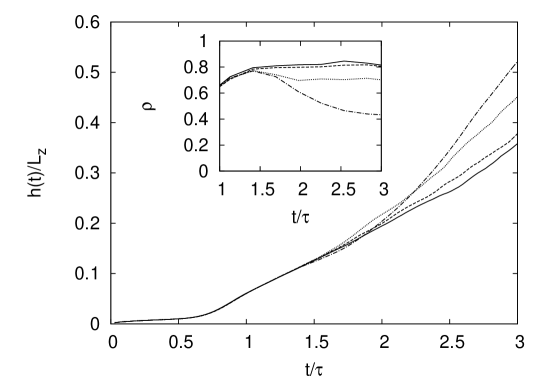
Figure 4: Temporal evolution of the mixing layer width $h(t)$. Inset: fraction of mixed fluid within the mixing layer $\rho=1/(L_{x}L_{y}L_{z})\int d^{3}x\theta[(r\theta_{0}/2)^{2}-T^{2}]$. Newtonian flow: solid line. Viscoelastic flows: dashed line (Run A), dotted line (Run B), dash-dotted line (Run C).

Figure 5: Time evolution of the ratio $w_{rms}/u_{rms}$ (panel a) and velocity gradients (panel b). Correlation length of vertical ($R_{w}$, panel c) and horizontal ($R_{u}$, panel d) velocity components. Newtonian flow: solid line. Viscoelastic flows: dashed line (Run A), dotted line (Run B).

In the viscoelastic solution the growth of the mixing layer is faster than in the Newtonian case (see Fig. 4), and the acceleration effect is stronger for polymers with longer relaxation times. On a coarse scale this effects produces a mixing enhancement. On the other hand, the viscoelastic fluid is less uniformly mixed within the mixing layer itself. In the Newtonian case the volume of the region where $|T({\bf x},t)|<r\theta_{0}/2$ is roughly $80\%$ of the volume of the mixing layer at the same time. Conversely, the fraction of mixed fluid within the mixing layer reduces up to $50\%$ for the viscoelastic case (see inset of Fig. 4). These results indicate that the effects of polymers on the mixing efficiency is twofold. At large scale they enhance the mixing by accelerating the growth of the mixing layer and at small scale they reduce the mixing efficiency of the turbulent flow.

These effects are accompanied by an increase of the anisotropy of the flow. In Figure 5 we show the ratio between rms of vertical ($w_{r}ms$) and horizontal velocities ($u_{r}ms$) and velocity gradients. The velocity ratio, which is around $1.8$ for the Newtonian case bmmv_pre09 , becomes larger than $2.5$ for the viscoelastic run. This phenomenon is associated with the enhancement of the vertical velocity of the mixing layer. The reduction of small-scale mixing efficiency results in the persistence of anisotropy also at small scales (i.e. in the velocity gradients), at variance with the Newtonian case in which it is almost absent. The viscoelastic flow is therefore characterized by the presence of faster and larger plumes than those characterizing the Newtonian case. The increased coherence of thermal plumes can be quantified in terms of the enhancement of the velocity correlation length (here defined as the half width of the velocity correlation function vc_pof09 ), of both horizontal and vertical velocity components (see Fig. 5).

V Interpretation in terms of drag reduction

The energy balance of the viscoelastic RT system differs from the Newtonian case because of the elastic contribution to the energy and dissipation. The energy can be written as the sum of potential, kinetic and elastic contributions:

$$E=P+K+\Sigma=-\beta g\langle zT\rangle+\frac{1}{2}\langle u^{2}\rangle+\frac{\nu\eta}{\tau_{p}}\left[\langle tr\sigma\rangle-3\right]$$ (2)

and the energy balance reads:

$${dE\over dt}=-\varepsilon_{\nu}-\varepsilon_{\Sigma}$$ (3)

where $\varepsilon_{\nu}=\nu\langle(\partial_{\alpha}u_{\beta})^{2}\rangle$ is the viscous dissipation and the last term represents elastic dissipation $\varepsilon_{\Sigma}=2\Sigma/\tau_{p}$. The evolution of the system is sustained by the consumption of potential energy, which provides a power source $-{dP\over dt}=\beta g\langle wT\rangle$ (where $w$ is the vertical velocity component). It is worth noting that the rate of energy injection is not determined a priori. Indeed, it is the dynamics itself which determines the rate of conversion of potential energy into kinetic and elastic energy. Our numerics reveals that polymers accelerate this process (see Fig. 6), and that kinetic energy for viscoelastic runs is larger than that of the Newtonian case (of about $40\%$ at $t=3.5\tau$). We remark that the faster growth of kinetic energy is not a straightforward consequence of the speed-up of potential energy consumption, due to the accelerated growth of mixing layer. Part of the potential energy is indeed converted into elastic energy and finally dissipated by polymers relaxation to equilibrium.

Figure 6: Temporal evolution of the potential energy $P$ (panel a), kinetic energy $K$ panel (b), elastic energy $\Sigma$ (panel c) and viscous energy dissipation (panel d). Newtonian flow: solid line. Viscoelastic flows: dashed line (Run A), dotted line (Run B).

Figure 7: Time evolution of the drag reduction factor $f$. Newtonian flow: solid line. Viscoelastic flows: dashed line (Run A), dotted line (Run B), dash-dotted line (Run C).

Figure 8: Energy spectra of the vertical velocity component at time $t=3.1\tau$ Newtonian flow: solid line. Viscoelastic flows: dashed line (Run A), dotted line (Run B), dash-dotted line (Run C).

The increase of kinetic energy is accompanied by a reduction of viscous dissipation (Fig. 6d). This is a clear fingerprint of a drag reduction phenomenon as defined for homogeneous-isotropic turbulence bdgp_pre03 ; dcbp_jfm05 , i.e. a reduction of turbulent energy dissipation at given kinetic energy. In the present case, a quantitative measure of the drag reduction is provided by the ratio between the loss of potential energy and the resulting plumes kinetic energy. The first can be easily computed by the definition of the potential energy $P=-\beta g\langle zT\rangle$ assuming a linear temperature profile within the mixing layer, which gives $\Delta P=P(0)-P(t)\simeq 1/6Agh(t)$. An estimate of the kinetic energy associated with large scale plumes can be obtained in terms of the mixing layer growth rate $\dot{h}(t)$ as $K_{L}\sim 1/2(\dot{h}(t))^{2}$. We remark that a similar estimation was proposed by Fermi for modeling the growth of mixing layer (see Appendix). The drag reduction coefficient $f$ is then defined as

$$f=\frac{\Delta P}{K_{L}}=1/3Ag\frac{h}{\dot{h}^{2}}=\frac{1}{12\alpha}$$ (4)

which turns out to be inversely proportional to the coefficient $\alpha$ which characterizes the mixing layer growth rate cc_natphys06 . With this definition, we measure $22\%$ of drag reduction for the viscoelastic run B and $30\%$ for the run C (see Fig. 7)

The scenario which emerges from these results is that polymers reduce the turbulent drag between rising and sinking plumes. The RT viscoelastic system is therefore able to convert more efficiently potential energy into kinetic energy contained in large plumes. Conversely, the turbulent transfer of kinetic energy to small-scale structures is reduced, which results in a reduction of the viscous energy dissipation. This picture is confirmed by the inspection of the energy spectra (see Fig. 8). At small scales we found a suppression of turbulent kinetic energy with respect to the Newtonian case, while at large scale an increase of the kinetic energy is observed.

The drag reduction scenario therefore provides a clear interpretation of the effects observed on the mixing properties. The enhancement of large-scale mixing associated with the faster growth of the mixing layer is directly connected to the reduced friction between plumes, and the reduced efficiency of small-scale mixing is a natural consequence of the suppression of small-scale turbulence.

The accelerated nature of the RT turbulence poses an interesting question about the existence of an asymptotic state for viscoelastic RT. For the Newtonian case the phenomenological theory assumes that in the late stage of the evolution all terms in the energy balance (3) have the same temporal scaling determined by gravity forces. This implies that $-{dP\over dt}\sim\varepsilon_{\nu}\sim t$ and $K\sim t^{2}$. In the viscoelastic case it is not possible to fix a priori the scaling law for the elastic contribution, because elastic energy $\Sigma$ is proportional to the elastic dissipation rate $\varepsilon_{\Sigma}=2\Sigma/\tau_{p}$. Assuming that the latter has the same temporal scaling than the viscous dissipation, $\varepsilon_{\nu}\sim\varepsilon_{\Sigma}\sim t$, one gets that the elastic contribution to the total energy should become negligible at long times. On the other hand, the assumption that elastic and kinetic energy have the same scaling $\Sigma\sim K\sim t^{2}$ leads to the conclusion that elastic dissipation would eventually dominate over the viscous one. Our simulations support the second hypothesis: the ratio between elastic end viscous dissipation is not constant, and grows almost linearly in time (see Fig. 9). A deeper investigation of this asymptotic state in which polymers are strongly elongated would require to go beyond Oldroyd-B model, and to adopt more realistic polymer model (e.g. FENE-P model) which accounts for maximal elongation and non-linear relaxation.

Figure 9: Temporal evolution of the ratio between elastic and viscous dissipation. Run A: dashed line. Run B: dotted line.

VI Heat transport enhancement

Figure 10: Temporal evolution of Nusselt number $Nu=\langle wT\rangle h/(\kappa\theta_{0})$. Inset: Nusselt number vs. Rayleigh number $Ra=Agh^{3}/(\nu\kappa)$. Newtonian flow: solid line. Viscoelastic flows: dashed line (Run A), dotted line (Run B), dash-dotted line (Run C).

Figure 11: Temporal evolution of the contributions to the heat transfer efficiency. Panel (a): Mixing layer width $h(t)$. Panel (b): Rms vertical velocity $w_{rms}$. Panel (c): Rms temperature $T_{rms}$. Panel (d): Correlation between temperature and vertical velocity $C_{wT}(z,t)$. Newtonian flow: solid line. Viscoelastic flows: dashed line (Run A), dotted line (Run B).

The heat transport efficiency in turbulent convection is usually measured by the Nusselt number $Nu=\langle wT\rangle h/(\kappa\theta_{0})$, which represents the ratio between convective and conductive heat transport. For a developed turbulent flow the Nusselt number is expected to behave as a simple power law with respect to the dimensionless temperature jump which defines the Rayleigh number $Ra=Agh^{3}/(\nu\kappa)$ gl_jfm00 . For a flow in which boundary layers are irrelevant, as in our case, Kraichnan kraichnan62 predicted many years ago an asymptotic regime which is expected to emerge at very large $Ra$. For this so-called ultimate state regime of thermal convection dimensional analysis predicts the scaling laws gl_jfm00

$$Nu\simeq Pr^{1/2}Ra^{1/2}\qquad Re\simeq Pr^{-1/2}Ra^{1/2}\,.$$ (5)

For the case of time dependent RT turbulent convection, all these dimensionless quantities depend on time. Dimensionally estimation gives (for the Newtonian case) $Ra\simeq(\beta g\theta_{0})^{4}t^{6}/(\nu\kappa)$, $Re\simeq(\beta g\theta_{0})^{2}t^{3}/\nu$ and $Nu\simeq(\beta g\theta_{0})^{2}t^{3}/\kappa$, which indeed imply the scaling laws (5) and which have been observed recently in numerical simulation of RT turbulence bmmv_pre09 ; bdm_prl10 .

The addition of polymers strongly enhances the efficiency of heat transport, i.e. the Nusselt number grows faster both as a function of time and as a function of $Ra$ bmmv_prl10 , and the effects increase with the polymer relaxation time, as shown in Fig. 10. In order to identify the different causes which contribute to this effect, it is useful to rewrite the Nusselt number as:

$$Nu=\frac{1}{\kappa\theta_{0}}hw_{rms}T_{rms}C_{wT}$$ (6)

where $C_{wT}=\langle wT\rangle/(w_{rms}T_{rms})$ is the correlation between the vertical velocity component and the temperature field. In the four panels of Fig. 11 we plot the four contributions $h$ (panel a) $w_{rms}$ (panel b), $T_{rms}$ (panel c) and $C_{wT}$ (panel d) as a function of time. It is evident that the increased heat transfer is not simply a consequence of the faster evolution of the mixing layer $h$, but also of the increased rms of the vertical velocity component, $w_{rms}$. Moreover, the reduction of small-scale turbulent mixing causes an increase of the temperature fluctuations $T_{rms}$ which also gives a positive contribution to the Nusselt number. Finally, in the viscoelastic case we found stronger correlations between temperature and vertical velocity component which therefore transport heat more efficiently. In conclusion, the increased heat transport efficiency is a combined effect of different contributions: the presence of faster thermal plumes, the reduced turbulent mixing, and the stronger correlation between thermal plumes and the vertical velocity component. While the first contribution is distinctive of RT turbulence, the others could in principle be observed in other thermal convective systems. A recent experiment performed within the framework of Rayleigh-Benard convection indicates in that case an opposite effect of heat transfer reduction an_prl10 but this can be probably attributed to the moderate stretching of polymers in that case.

VII Conclusions

The behavior of viscoelastic flows in the RT setup provides the first clear evidence of simultaneous occurrence of both polymer drag reduction and heat transport enhancement. Drag reduction in this system is caused by a reduced drag between rising and sinking thermal plumes, a fact which implies the speed up of the mixing layer growth. This process shares many analogies with drag reduction observed in homogeneous, isotropic turbulence, namely the suppression of small-scale turbulence which results in a reduced viscous drag. These analogies provide a support to the conjecture of a common underlying mechanisms behind these different manifestations of the polymer drag reduction in bulk flows.

For RT system it is possible to introduce a drag coefficient in terms of the ratio between the potential energy loss which forces the flow, and the resulting kinetic energy associated with thermal plumes. The viscoelastic case is characterized by faster and more coherent thermal plumes. The effects on mixing is to enhance the large-scale mixing, and to reduce the small-scale one. As a consequence, the drag coefficient is reduced and the heat transport efficiency, measured by the Nusselt number, is increased.

We conclude with some speculations on the possible observation of heat transfer enhancement in laboratory experiments. The values of the parameters used in our simulations can be used to determine the setup for a comparable experiments. The units of time $T$ and length $L$ which allow one to convert the parameters of our simulations into physical quantities can be fixed by matching the numerical values of viscosity $\tilde{\nu}=3\cdot 10^{-4}$ and gravity $\tilde{g}=(4A)^{-1}$ used in our simulations with physical values $g=9.81ms^{-2}$, $\nu=\nu_{H_{2}O}=10^{-6}m^{2}s^{-1}$:

$$L^{3} = \frac{\tilde{g}}{\tilde{\nu}^{2}}\frac{\nu^{2}}{g}$$ (7)

$$T^{3} = \frac{\tilde{g}^{2}}{\tilde{\nu}}\frac{\nu}{g^{2}}$$ (8)

By choosing the Atwood number $A=0.1$ one gets $L\simeq 1.4cm$ and $T\simeq 0.06s$. This correspond to an experimental box of $L_{x,y}\simeq 10cm$ and $L_{z}\simeq 20cm$, and polymer relaxation times $\tau_{p}=60ms$ for the case A, which is close to realistic relaxation times of long-chain polymers in water. The evolution of the system will be quite fast: the time required for the mixing layer to invade the whole box is estimated to be roughly $2s$. Let us notice that the limit of small Atwood number, required in the present study to justify the Boussinesq approximation, is not a constraint for an experimental setup, where large values of $A$ can be obtained by means of some additives (e.g. salt) to generate density differences. It would be interesting to observe experimentally the influence of non-Boussinesq effects on the drag reduction phenomenon.

Appendix A Fermi model for the growth of mixing layer

Enrico Fermi, together with John von Neumann, were probably the first who considered a model for the growth of mixing layer in the nonlinear stage. The model is described in two reports of the Los Alamos Scientific Laboratory, the first from September 1951 (Fermi alone) and the second from August 1953 (Fermi and von Neumann) never published fv_lanl55 . The idea of this work, in the words of the authors, is to “discuss in a very simplified form the problem of the growth of an initial ripple on the surface of an incompressible liquid in presence of an acceleration”. The first report of Fermi considers the interface between a liquid and vacuum, while the second report with von Neumann analyzes the case of two fluids of different densities.

Figure 12: Fermi’s model for the evolution of the interface. The smooth interface $ACE^{\prime}$ is replaced by the square wave $ABCEE^{\prime}$.

The idea of Fermi is to approximate the interface with a square wave whose shape is characterized by three parameters: the heights of spike and bubble $a$ and $b$ and the width of the spike $x$ (see Fig. 12). Incompressibility gives a relation among these quantities, $b=ax/(1-x)$. Fermi next considers the Euler-Lagrange equations for the variation of the potential and kinetic energy and obtains a couple of equations for the evolution of $a$ and $x$. In the following we consider a simplified version of Fermi model with bubble-spike symmetry ($b=a$, $x=1/2$), consistent with the Boussinesq approximation discussed in the present paper.

The variation of potential energy to generate the profile in Fig. 12 is

$$U={\rho_{2}-\rho_{1}\over 2}gL_{x}L_{y}a^{2}$$ (9)

For the kinetic energy, assuming that the “plumes” $ABCO$ and $CC^{\prime}E^{\prime}E$ move respectively up and down with velocity $\dot{a}$ and plumes $BB^{\prime}C^{\prime}C$ and $OCED$ move respectively right and left with the same velocity (for incompressibility) one obtains

$$K={\rho_{1}+\rho_{2}\over 2}L_{x}L_{y}a\dot{a}^{2}$$ (10)

From the Lagrange equations

$${d\over dt}{\partial K\over\partial\dot{a}}-{\partial K\over\partial a}=-{\partial U\over\partial a}$$ (11)

one the obtains a differential equation for the $a(t)$ without free parameter. We remark that (11) assumes that all potential energy is transformed in large scale kinetic energy generating the motion of the interface. In a later stage, in which a turbulent flow develops, we can still try to use (11) but now with a factor $0\leq\delta\leq 1$ in front of the rhs which takes into account that a fraction ($1-\delta$) of potential energy goes in viscous dissipation (through the turbulent cascade). With this correction the equation for $a(t)$ reads

$${d^{2}a\over dt^{2}}a+{1\over 2}\left({da\over dt}\right)^{2}={1\over 4}\delta Aga$$ (12)

Introducing the width of the interface $h(t)=2a(t)$ and solving (12) with initial condition $h(0)=h_{0}$ and replacing $\delta\equiv 8\alpha$ we finally get

$$h(t)=h_{0}+(4\alpha Agh_{0})^{1/2}t+\alpha Agt^{2}$$ (13)

which is the form proposed from other authors on the basis of completely different considerations rc_jfm04 ; cc_natphys06 .

References

- (1) B. A. Toms, Proc. 1st International Congress on Rheology 2, 135 (1949)
- (2) G. Boffetta, A. Celani, and A. Mazzino, Phys Rev E 71, 036307 (2005)
- (3) A. Bistagnino, G. Boffetta, A. Celani, A. Mazzino, A. Puliafito, , and M. Vergassola, J. Fluid Mech. 590, 61 (2007)
- (4) R. Benzi, E. De Angelis, R. Govindarajan, and I. Procaccia, Phys. Rev. E 68, 016308 (Jul 2003)
- (5) E. De Angelis, C. M. Casciola, R. Benzi, and R. Piva, J. Fluid Mech. 531, 1 (2005)
- (6) S. Berti, A. Bistagnino, G. Boffetta, A. Celani, and S. Musacchio, Europhys. Lett. 76, 63 (2006)
- (7) G. Boffetta, A. Mazzino, S. Musacchio, and L. Vozella, J. Fluid Mech. 643, 127 (2010)
- (8) G. Boffetta, A. Mazzino, S. Musacchio, and L. Vozella, Phys. Rev. Lett. 104, 184501 (2010)
- (9) R. B. Bird, O. Hassager, R. C. Armstrong, and C. F. Curtiss, Dynamics of Polymeric Liquids (Wiley-Interscience, 1987)
- (10) R. Sureshkumar and A. Beris, J. Non-Newtonian Fluid Mech. 60, 53 (1995)
- (11) M. Chertkov, Phys. Rev. Lett. 91, 115001 (Sep 2003)
- (12) N. Vladimirova and M. Chertkov, Phys. Fluids 21, 015102 (2008)
- (13) G. Boffetta, A. Mazzino, S. Musacchio, and L. Vozella, Phys. Rev. E 79, 065301 (2009)
- (14) A. Celani, A. Mazzino, and L. Vozella, Phys. Rev. Lett. 96, 134504 (2006)
- (15) P. Ramaprabhu and M. Andrews, Phys. Fluids 16, L59 (2004)
- (16) G. Dimonte, D. L. Youngs, A. Dimits, S. Weber, M. Marinak, S. Wunsch, C. Garasi, A. Robinson, M. J. Andrews, P. Ramaprabhu, et al., Phys. Fluids 16, 1668 (2004)
- (17) K. Kadau, C. Rosenblatt, J. L. Barber, T. C. Germann, Z. Huang, P. Carlès, and B. J. Alder, Proc. Nat. Acad. Sci. 104, 7741 (2007)
- (18) M. J. Andrews and D. B. Spalding, Phys. Fluids A 2, 922 (1990)
- (19) S. Dalziel, P. Linden, and D. Youngs, J. Fluid Mech. 399, 1 (1999)
- (20) W. H. Cabot and A. W. Cook, Nature Physics 2, 562 (2006)
- (21) S. Grossmann and D. Lohse, J. Fluid Mech. 407, 27 (2000)
- (22) R. H. Kraichnan, Phys. Fluids 5, 1374 (1962)
- (23) G. Boffetta, F. De Lillo, and S. Musacchio, Phys. Rev. Lett. 104, 034505 (2010)
- (24) G. Ahlers and A. Nikolaenko, Phys. Rev. Lett. 104, 034503 (2010)
- (25) E. Fermi and J. von Neumann, Internal Report, US Atomic Energy Commission AECU-2979 (1955)
- (26) J. Ristorcelli and T. Clark, J .Fluid Mech. 507, 213 (2004)