Free-energy functional for freezing transitions: Hard sphere systems freezing into crystalline and amorphous structures

Abstract

A free-energy functional that contains both the symmetry conserved and symmetry broken parts of the direct pair correlation function has been used to investigate the freezing of a system of hard spheres into crystalline and amorphous structures. The freezing parameters for fluid-crystal transition have been found to be in very good agreement with the results found from simulations. We considered amorphous structures found from the molecular dynamics simulations at packing fractions $\eta$ lower than the glass close packing fraction $\eta_{J}$ and investigated their stability compared to that of a homogeneous fluid. The existence of free-energy minimum corresponding to a density distribution of overlapping Gaussians centered around an amorphous lattice depicts the deeply supercooled state with a heterogeneous density profile.

I Introduction

When a liquid freezes into a crystalline solid its continuous symmetry of translation and rotation is broken into one of the Bravais lattices. In three dimensions the freezing of a liquid into a crystalline solid is known to be first-order symmetry breaking transition marked by large discontinuities in entropy, density and order parameters. The molecules in a crystal are localized on a lattice described by a discrete set of vectors $\{{\bf{R}}_{i}\}$ such that any functions of position, such as one particle density $\rho({{\bf r}})$ satisfies $\rho({\bf r})=\rho({\bf r}+{\bf{R}}_{i})$ for all ${\bf{R}}_{i}$ $[1]$. This set of vectors necessarily forms a Bravais lattice. But when the liquid is supercooled bypassing its crystallization, it continues to remain in amorphous state. With increase in density a solid like phase emerges with molecules getting localized around their mean position on a random structure. The underlying lattice on which such localized motion takes place is related to the time scale of relaxation in the supercooled liquid. While the supercooled liquid starts to attain solidlike properties, structurally it does not have any long range order like the one present in the crystal. This phenomena is termed the “glass transition” $[2,3]$. Although the glassy materials are well characterized experimentally, the existence of phase transition into the glassy state remains controversial $[4-6]$. Our aim in this paper is not to enter in this discussion but to examine the stability (metastability) of amorphous structures from a thermodynamic point of view, using the standard method of density-functional theory which is also used to investigate the crystallization of liquids. We refer to glassy or amorphous solid a structure in which particles are localized around their mean positions forming a random lattice. Localization of particles amounts to breaking of continuous translational symmetry of normal liquid and takes place in forming both crystals and glasses.

The structural properties of a classical system can adequately be described by one and two-particle density distributions. The one particle density distribution $\rho({\bf r})$ defined as

$$\rho({\bf r})=\langle\sum_{k}\delta{({\bf r}-{\bf{R}}_{k})}\rangle$$ (1)

where $\bf{R}_{k}$ is the position vector of k-th particle and bracket $\langle....\rangle$ represents the ensemble average, is constant independent of position for an isotropic liquid, but contains most of the structural informations of crystals and glasses. The particle density distribution $\rho^{(2)}({\bf r}_{1},{\bf r}_{2})$ which gives the probability of finding simultaneously a molecule in a volume element $d{\bf r}_{1}$ centered at ${\bf r}_{1}$ and a second molecule in volume element $d{\bf r}_{2}$ centered at ${\bf r}_{2}$ is defined as

$$\rho^{(2)}({\bf r}_{1},{\bf r}_{2})=\langle\sum_{j}\sum_{\neq k}\delta{({\bf r}_{1}-\bf{R}_{j})}\delta{({\bf r}_{2}-\bf{R}_{k})}\rangle$$ (2)

The pair correlation function $g{({\bf r}_{1},{\bf r}_{2})}$ is related to $\rho^{(2)}({\bf r}_{1},{\bf r}_{2})$ by the relation

$$g({\bf r}_{1},{\bf r}_{2})=\frac{\rho^{(2)}({\bf r}_{1},{\bf r}_{2})}{\rho({\bf r}_{1})\rho({\bf r}_{2})}$$ (3)

The direct pair correlation function $c({\bf r}_{1},{\bf r}_{2})$ which appears in the expression of free-energy functional (see Sec. $II$) is related to the total pair correlation function $h({\bf r}_{1},{\bf r}_{2})=g({\bf r}_{1},{\bf r}_{2})-1$ through the Ornstein-Zernike (OZ) equation,

$$h({\bf r}_{1},{\bf r}_{2})=c({\bf r}_{1},{\bf r}_{2})+\int{c({\bf r}_{1},{\bf r}_{3})\rho({\bf r}_{3})h({\bf r}_{2},{\bf r}_{3})d{\bf r}_{3}}$$ (4)

Since in an isotropic liquid $\rho({\bf r}_{1})=\rho({\bf r}_{2})=\rho_{l}=N/V$ where $N$ is the average number of molecules in volume $V$,

$$g(r)=\frac{\rho^{(2)}({\bf r}_{1},{\bf r}_{2})}{\rho^{(2)}_{l}}$$ (5)

where $r=|{\bf r}_{2}-{\bf r}_{1}|$. In a liquid of spherically symmetric particles $g({\bf r}_{1},{\bf r}_{2})$, $h({\bf r}_{1},{\bf r}_{2})$, $c({\bf r}_{1},{\bf r}_{2})$ depend only on interparticle separation $r=|{\bf r}_{2}-{\bf r}_{1}|$. This simplification is due to homogeneity which implies continuous translational symmetry and isotropy which implies continuous rotational symmetry. Such simplification does not, in general, occur in frozen phases. We refer crystal as well as glass as frozen phases. While a crystal is both inhomogeneous and anisotropic, a glass can be regarded as isotropic but inhomogeneous. The heterogeneity in glassy system over length and time scales has been studied in several recent works $[7]$ related to computer simulations.

The total and direct pair correlation functions of a system can be given as a simultaneous solution of the OZ equation and a closure relation that relates the correlation functions to the pair potential. Well known closure relations are the Percus-Yevick (PY) relation, the hypernatted chain (HNC) relation and the mean spherical approximation (MSA). It may, however, be noted that while the OZ equation $(1.4)$ is general and connects the total and direct pair correlation functions of liquids as well as of frozen phases, the closure relations have been derived assuming translational invariance $[8]$ and therefore valid only to normal fluids. The integral equation theory has been used quite successfully to describe the structure of isotropic liquids. But its application to frozen phases has so far been very limited $[9,10]$. In Sec. $III$ we describe a method to calculate the DPCF of frozen phases formed by breaking of continuous translational symmetry of liquids and use it in a free-energy functional described in Sec. $II$ to study freezing transitions in Sec. $IV$ and $V$.

Since its advent in 1979 by Ramakrishnan and Yussouff (RY) $[11]$, the density functional theory (DFT) has been applied to freezing transition of variety of pure liquids and mixtures $[11,12]$. A DFT requires an expression of the Halmholtz free-energy (or grand thermodynamic potential) in terms of one- and two-particle distribution functions and a relation that relates $\rho({\bf r})$ to pair correlation functions. Such a relation is formed by minimizing the free-energy with respect to $\rho({\bf r})$ with appropriate constraints $[12,13]$. The DPCF that appear in these equations are of frozen phase and are functional of $\rho({\bf r})$. When this functional dependence is ignored and the DPCF is replaced by that of the co-existing isotropic liquid $[11]$ or by an “effective fluid” $[14]$ the free-energy functional becomes approximate and fails to provide an accurate description of freezing transitions and stability of frozen phases. An improved free-energy functional which contains both the symmetry conserved and symmetry broken parts of the DPCF has recently been developed $[9,10]$ and applied to study the isotropic-nematic transition $[9]$ and the crystallization of power-law fluids $[10]$.

In this paper we investigate the freezing of fluids of hard sphere into crystalline and amorphous phases and compare our results with the results of previous investigations. Hard spheres are ubiquitous in condensed matter; they have been used as models of liquids, crystals, colloidal systems, granular systems and powders. Packing of hard spheres are of even wider interest as they are related to important problems in information theory, such as diagonalization of signals, error correcting codes, and optimization problems $[15]$. Recently, amorphous packing of hard spheres have attracted much attention $[6,16-18]$ because for polydisperse colloids and granular materials the crystalline state is not obtained for kinetic reasons . It is therefore necessary to have a statistical-mechanical theory based on first principle which can correctly describe the freezing of hard spheres.

The paper is organized as follows: In Sec. $II$ we describe the free-energy functional for a symmetry broken phase which contains both the symmetry conserving and symmetry broken parts of direct pair correlation functions. In Sec. $III$ we describe a method to calculate these correlation functions. The theory is applied in Sec. $IV$ to investigate the freezing of fluids into crystalline solids and in Sec. $V$ the metastability of amorphous structures.

II Free-energy functional

An important step in construction of the density functional model of a frozen phase is proper parametrization of extremely inhomogeneous density function $\rho({\bf r})$ which value near a lattice site may be orders of magnitude higher than in the interstitial regions. One very successful prescription of $\rho({\bf r})$ is as a collection of overlapping Gaussian profiles $[19]$ centered over a set of lattice sites ${\bf{R}}_{m}$.

$$\rho({\bf r})=\sum_{m}(\frac{\alpha}{\pi})^{3/2}exp\left[-\alpha{\left({\bf r}-{\bf{R}}_{m}\right)}^{2}\right]$$ (6)

The width of a Gaussian profile is inversely proportional to the square root of $\alpha$ which will be referred to as localization parameter. In this representation, the limit $\alpha\rightarrow 0$ is the homogeneous liquid state and higher values of $\alpha$ represent increasingly localized structures.

Taking Fourier transform of $(2.1)$ one gets

$$\rho({\bf r})=\rho_{0}+\frac{1}{V}\sum_{q\neq 0}\rho_{q}e^{i\bf{q}\cdot{\bf r}}$$ (7)

where

$$\rho_{q}=e^{-{q^{2}}/4\alpha}\sum_{n}e^{-i\bf{q}\cdot{\bf{R}}_{n}}$$ (8)

is amplitude of density wave of wavelength $2\pi/|q|$. The nature and magnitude of inhomogeneity of a frozen phase is measured by $\rho_{q}$ which will be referred to as order parameter; $\rho_{q}=0$ for $q\neq 0$ corresponds to isotropic fluid and $\rho_{q}\neq 0$ to a frozen phase. For a crystal in which ${{\bf{R}}_{m}}$ forms a periodic lattice, $e^{i\bf{q}\cdot\bf{R}_{m}}=\delta_{\bf{q},\bf{G}}$ where $\bf{G}$ are reciprocal lattice vectors (R. L. V.), Eq.$(2.2)$ reduces to

$$\rho_{s}({\bf r})=\rho_{0}+\rho_{0}\sum_{G}e^{-G^{2}/4\alpha}e^{i\bf{G}\cdot{\bf r}}$$ (9)

This is a well known expression of $\rho({\bf r})$ of a crystal. As in an amorphous or glassy structure the lattice sites are randomly distributed and are not known, the above simplification is not possible. We can, however, calculate and have an idea of inhomogeneity and its difference from that of a crystalline solid using the distribution of $\bf{R}_{n}$ determined from numerical simulations $[20,21]$. Thus

$$\rho_{g}(r)=\rho_{0}+\frac{1}{V}\sum_{q\neq 0}e^{-{q^{2}}/{4\alpha}}\left[1+\rho_{0}\left(\int d{\bf{R}}h(R)e^{-i{\bf{q}}\cdot{\bf{R}}}\right)\right]e^{i{\bf{q}}\cdot{\bf{r}}}$$ (10)

where $g(R)=1+h(R)$ is the site-site correlation function which provides the structural description of amorphous structure. In Fig.$1$ we plot $\rho_{g}({\bf r})$ for $\eta(\equiv\frac{1}{2}\pi\rho_{0}{\sigma}^{3};\sigma$ being the diameter particle)$=0.576$ and $\alpha=150$ (highly localized condition) and $\alpha=15$ (weakly localized condition). In calculating $\rho_{g}(r)$ we used $g(R)$ data found for amorphous structures of granular particles [21] shown in Fig.$2$. In Fig.$2$ we also show the value of $g(R)$ of a liquid found from solving the integral equations discussed in Sec. $III$, for comparison. From Fig.$1$ we see that while inhomogeneity increases with value of $\alpha$, unlike crystalline solid, it remains confined to about $4$ particle diameter, even for $\alpha=150$ and decays rapidly on increasing the distance.

The reduced free-energy $A[\rho]$ of an inhomogeneous system is a functional of $\rho({\bf r})$ and is written as

$$A[\rho]=A_{id}[\rho]+A_{ex}[\rho]$$ (11)

The ideal gas part is exactly known and is given as

$$A_{id}[\rho]=\int d{\bf r}\rho({\bf r})\left[ln\left(\rho({\bf r})\Lambda\right)-1\right]$$ (12)

where $\Lambda$ is cube of the thermal wavelength associated with a molecule. The excess part arising due to intermolecular interactions is related to the DPCF as $[9,10]$

$$\frac{\delta^{2}A_{ex}[\rho]}{\delta\rho({\bf r}_{1})\delta\rho({\bf r}_{2})}=-c^{(0)}({\bf r}_{1},{\bf r}_{2};\rho_{0})-c^{(b)}({\bf r}_{1},{\bf r}_{2};[\rho])$$ (13)

where superscripts $(0)$ and $(b)$ represent, respectively, the symmetry conserving and symmetry breaking parts of the DPCF. In other words $c^{(0)}$ is found by treating the system to be isotropic and homogeneous with density $\rho_{0}$ whereas $c^{(b)}$ are the contribution which arise due to heterogeneity in density in a frozen phase.

$A_{ex}[\rho]$ is found by functional integration of Eq.$(2.8)$. In this integration the system is taken from some initial density to the final density $\rho({\bf r})$ along a path in the density space; the result is independent of the path of integration. As the symmetry conserving part $c^{(0)}$ is function of density the integration in the density space is done taking an isotropic fluid of density $\rho_{0}$ (or $\rho_{l}$, the density of co-existing fluid in case of crystal) as reference.This leads to

$$A_{ex}^{(0)}[\rho]=A_{ex}(\rho_{0})-\frac{1}{2}\int d{\bf r}_{1}\int d{\bf r}_{2}\Delta\rho({\bf r}_{1})\Delta\rho({\bf r}_{2})c^{(0)}(r)$$ (14)

where $\Delta\rho({\bf r}_{1})=\rho({\bf r}_{1})-\rho_{0}$ and $A_{ex}(\rho_{0})$ is the excess reduced free-energy of an isotropic system of density $\rho_{0}$.

The integration over $c^{(b)}$ has to be done in the density space spanned by the number density $\rho_{0}$ and order parameters $\rho_{q}$. We characterize this part of the density space by two parameters $\lambda$ and $\xi$ which vary from $0$ to $1$. The parameter $\lambda$ raises the density from $0$ to $\rho_{0}$ as it varies from $0$ to $1$ whereas the parameter $\xi$ raises the order parameters from $0$ to $\rho_{q}$ for each value of q. This gives $[9,10]$.

$$A^{(b)}_{ex}[\rho]=-\frac{1}{2}\int d{\bf r}_{1}\int d{\bf r}_{2}\Delta\rho({\bf r}_{1})\Delta\rho({\bf r}_{2})\bar{c}^{(b)}\left({\bf r}_{1},{\bf r}_{2};[\rho]\right)$$ (15)

where

$$\bar{c}^{(b)}({\bf r}_{1},{\bf r}_{2};[\rho])=4\int_{0}^{1}d\xi\xi\int_{0}^{1}d\xi^{{}^{\prime}}\int_{0}^{1}d\lambda\lambda\int_{0}^{1}d\lambda^{{}^{\prime}}c^{(b)}({\bf r}_{1},{\bf r}_{2};\lambda\lambda^{{}^{\prime}}\rho_{0};\xi\xi^{{}^{\prime}}\rho_{q})$$ (16)

While integrating over $\lambda$ the order parameter $\rho_{q}$ are kept fixed and while integrating over $\xi$ the density is kept fixed. The result does not depend on the order of integration. The free-energy functional of a frozen phase is the sum of $A_{id}$, $\Delta A^{(0)}[\rho]$ and $\Delta A^{(b)}[\rho]$ given, respectively, by Eq.$(2.7)$,$(2.9)$ and $(2.10)$.

The minimization of $\Delta A=A[\rho]-A(\rho_{0})$ where $A(\rho_{0})$ is the free-energy of an homogeneous and isotropic system of density $\rho_{0}$, leads to

$$\ln\frac{\rho({\bf r})}{\rho_{0}}=\lambda+\int d{\bf r}_{2}\Delta\rho({\bf r}_{2})c^{(0)}(|{\bf r}_{2}-{\bf r}_{1}|,\rho_{0})+\int d{\bf r}_{2}\Delta\rho({\bf r}_{2})\tilde{c}^{(b)}({\bf r}_{1},{\bf r}_{2})$$ (17)

Here $\lambda$ is the Lagrange multiplier and is determined from the condition

$$\frac{1}{V}\int_{V}\frac{\rho(r)}{\rho_{0}}d{\bf r}=1$$ (18)

and

$$\tilde{c}^{(b)}({\bf r}_{1},{\bf r}_{2})=2\int_{0}^{1}d\lambda\int_{0}^{1}d\xi c^{(b)}({\bf r}_{1},{\bf r}_{2},\lambda\rho_{0},\xi\rho_{q})$$ (19)

In principle, the only information we need to know is the value of $c^{(0)}(r)$ and $c^{(b)}({\bf r}_{1},{\bf r}_{2};[\rho])$ to calculate self consistently the value of $\rho(r)$ which minimizes the free-energy. In practice, one, however, finds it convenient to do minimization for assumed form of $\rho({\bf r})$ $[12]$

III Calculation of Direct Pair Correlation Function

To calculate the values of $c^{(0)}(r)$ we use the integral equation theory consisting of OZ equation,

$$h^{(0)}(r)=c^{(0)}(r)+\rho_{0}\int d{\bf r}^{{}^{\prime}}c^{(0)}(r^{{}^{\prime}})h^{(0)}(|{\bf r}^{{}^{\prime}}-{\bf r}|)$$ (20)

and a closure relation proposed by Rogers and Young [22]. This closure relation is written as

$$1+h^{(0)}(r)=exp(-u(r)/k_{B}T)\left[1+\frac{exp(\gamma(r)f(r))-1}{f(r)}\right]$$ (21)

where

$$\gamma(r)=h(r)-c(r)$$ (22)

and

$$f(r)=1-exp(-\psi r)$$ (23)

Here $\psi$ is an adjustable parameter used to achieve thermodynamic consistency and its value for a system of hard spheres is found to be equal to $0.16$ $[22]$. In Eq.$(3.2)$ $u(r)$ is pair potential, $k_{B}$, the Boltzmann constant and T, temperature. This closure relation was found by mixing the PY and HNC closure relations in such a way that at $r=0$ it reduces to the PY approximation and for values of $r$ where $f(r)$ approaches $1$, it reduces to the HNC approximation. Eqs$(3.1)-(3.4)$ together constitute a thermodynamically consistent theory and has been found to give values of pair correlation functions which are in very good agreement with Monte Carlo results.

The differentiation of Eqs.$(3.1)$ and $(3.2)$ with respect to density yields the following two relations,

$$\frac{\partial h^{(0)(r)}}{\partial\rho_{0}}=\frac{\partial c^{(0)}(r)}{\partial\rho_{0}}+\int d{\bf r}^{{}^{\prime}}c^{(0)}(r^{{}^{\prime}})h^{0}(|{\bf r}^{{}^{\prime}}-{\bf r}|)+\rho_{0}\int d{\bf r}^{{}^{\prime}}\frac{\partial c^{(0)}}{\partial\rho_{0}}h^{(0)}(|{\bf r}^{{}^{\prime}}-{\bf r}|)+\rho_{0}\int d{\bf r}^{{}^{\prime}}c^{(0)}(r)\frac{\partial h^{(0)}(|{\bf r}^{{}^{\prime}}-{\bf r}|)}{\partial\rho_{0}}$$ (24)

and

$$\frac{\partial h^{(0)}(r)}{\partial\rho_{0}}=exp\left(-\frac{u(r)}{k_{B}T}\right)\left[exp\left[\gamma(r)f(r)\right]\frac{\partial\gamma(r)}{\partial\rho_{0}}\right]$$ (25)

The closed set of coupled equations $(3.1)$, $(3.2)$, $(3.5)$ and $(3.6)$ have been solved using Gillen’s algorithm $[23]$ for four unknowns $h^{(0)}$, $c^{(0)}$, $\frac{\partial h^{(0)}}{\partial\rho_{0}}$ and $\frac{\partial c^{(0)}}{\partial\rho_{0}}$. We compare the values of $c^{(0)}(r)$ at packing fractions $\eta=0.50$ and $0.55$ in Fig.$(3)$ and values of $\frac{\partial c^{(0)}(r)}{\partial\rho_{0}}$ for the same two values of $\eta$ in Fig.$(4)$ to see the density dependence of these functions. While $\eta=0.50$ is close to the value of packing fraction at which system freezes into a crystalline solid, $\eta=0.55$ is close to the value of packing fraction $\eta_{M}$ at which the crystal melts.

Since all closure relations (including the one given by Eq.$(3.2)$) which are used in the integral equation theory for pair correlation functions are derived assuming translational invariance $[8]$, their use in calculating the values of pair correlation function of frozen phases may not be appropriate. In view of this we use a series expansion in which the contribution to the the DPCF arising due to inhomogeneity of the system is expressed in terms of higher body direct correlation functions of the uniform (isotropic and homogeneous) system. Thus

$$c^{(b)}({\bf r}_{1},{\bf r}_{2};[\rho])=\int d{\bf r}_{3}c^{(0)}_{3}({\bf r}_{1},{\bf r}_{2},{\bf r}_{3};\rho_{0})(\rho({\bf r}_{3})-\rho_{0})+\int d{\bf r}_{3}d{\bf r}_{4}c^{(0)}_{4}({\bf r}_{1},{\bf r}_{2},{\bf r}_{3},{\bf r}_{4})(\rho({\bf r}_{3})-\rho_{0})(\rho({\bf r}_{4})-\rho_{0})+\cdots$$ (26)

where $\rho({\bf r}_{n})-\rho_{0}=\sum_{q\neq 0}\rho_{q}e^{i\bf{q}\cdot{\bf r}_{n}}$. In Eq.$(3.7)$ $c^{(0)}_{n}$ are n-body direct correlation functions of the uniform system which can be found using the relations

$$\frac{\delta c^{(0)}(r)}{\delta\rho_{0}}=\int d{\bf r}_{3}c^{(0)}_{3}({\bf r}_{1},{\bf r}_{2},{\bf r}_{3})$$ (27)

$$\frac{\delta^{2}c^{(0)}(r)}{\delta\rho_{0}^{2}}=\int d{\bf r}_{3}d{\bf r}_{4}c^{(0)}_{4}({\bf r}_{1},{\bf r}_{2},{\bf r}_{3},{\bf r}_{4})$$ (28)

etc. The values of derivatives of $c^{(0)}(r)$ appearing on l. h. s. of above equations have been found using the integral equation theory described above.

We note that Eq.$(3.7)$ satisfies the condition that $c^{(b)}$ is zero in the fluid phase and depends on the magnitude (order parameter) and phase factors of density waves. These density waves measure the nature and magnitude of inhomogeneity of frozen phases. While each wave contributes independently to the first term of Eq.$(3.7)$ interactions between the two waves contribute to the second term and so on. The contributions made by successive terms of Eq.$(3.7)$ depends on the range of pair potential $u(r)$ $[10]$. As the range of potential increases the contribution made by higher order terms increases. For a system of hard spheres we find that at the freezing transition the contributions made by first term to free-energy is already small and therefore higher terms are expected to be negligible; it is only for $u(r)\propto r^{-n},n<12$ the contribution made by second order term becomes important $[10]$. In view of fast convergence of the series, Eq.$(3.7)$ seems to be a useful expression for calculating $c^{(b)}({\bf r}_{1},{\bf r}_{2})$

The first term of Eq.$(3.7)$ involves three-body direct correlation function which can be factorized as a product of two-body functions $[24]$. Thus

$$c^{(0)}_{3}({\bf r}_{1},{\bf r}_{2},{\bf r}_{3};\rho_{0})=t(r_{12})t(r_{13})t(r_{23})$$ (29)

The function $t(r)$ is determined using relation of Eq. $(3.8)$

$$\frac{\partial c^{(0)}(r)}{\partial\rho_{0}}=t(r)\int d{\bf r}^{{}^{\prime}}t(r^{{}^{\prime}})t(|{\bf r}^{{}^{\prime}}-{\bf r}|)$$ (30)

We adopt the numerical procedure developed in [24] to calculate $t(r)$ from known values of $\frac{\delta c^{(0)}(r)}{\delta\rho_{0}}$ from $(3.11)$. The values of $t(r)$ are plotted in Fig.$(5)$ for $\eta=0.50$ and $0.55$ to show their density dependence.

Taking only the first term in Eq.$(3.7)$ we write,

$$c^{(b)}({\bf r}_{1},{\bf r}_{2})=\frac{1}{V}\sum_{q}\sum_{n}\mu_{q}\int d{\bf r}_{3}t(|{\bf r}_{3}-{\bf r}_{1}|)e^{i\bf{q}({\bf r}_{3}-\bf{R_{n}})}t(|{\bf r}_{3}-{\bf r}_{2}|)$$ (31)

where $\mu_{q}=e^{-q^{2}/4\alpha}$ Using the relation

$${\bf r}_{3}=\frac{1}{2}({\bf r}_{1}+{\bf r}_{2})-\frac{1}{2}({\bf r}_{2}-{\bf r}_{1})+({\bf r}_{3}-{\bf r}_{1})$$ (32)

we find that $c^{(b)}({\bf r}_{1},{\bf r}_{2})$ can be written in a Fourier series in the center of mass variable ${\bf r}_{c}=\frac{1}{2}|{\bf r}_{1}+{\bf r}_{2}|$ with coefficients that are functions of the difference variable ${\bf r}={\bf r}_{2}-{\bf r}_{1}$, i.e,

$$c^{(b)}({\bf r}_{1},{\bf r}_{2})=\frac{1}{V}\sum_{q}c^{(q)}({\bf r})e^{i\bf{q}\cdot{\bf r}_{c}}$$ (33)

where

$$c^{(q)}({\bf r})=\sum_{n}\mu_{q}e^{-i\bf{q}\cdot\bf{R_{n}}}e^{-\frac{1}{2}\bf{q}\cdot{\bf r}}\int d{\bf r}^{{}^{\prime}}t(r^{{}^{\prime}})e^{i\bf{q}\cdot{\bf r}^{{}^{\prime}}}t(|{\bf r}^{{}^{\prime}}-{\bf r}|)$$ (34)

Since the DPCF is real and symmetric with respect to the interchange of ${\bf r}_{1}$ and ${\bf r}_{2}$, $c^{(q)}({\bf r})=c^{(-q)}({\bf r})$ and $c^{(q)}({\bf r})=c^{(q)}(-{\bf r})$. For given value of $\alpha$ and ${\bf{R_{n}}}$ one can calculate $c^{(q)}(r)$ from known value of $t(r)$. We discuss our results for crystalline and amorphous solids in following sections.

IV Crystalline Solid

A. Calculation of $c^{(b)}({\bf r}_{1},{\bf r}_{2})$

For a crystal in which vectors ${\bf{R}_{n}}$ form a Bravais lattice $Eq.(3.14)$ and $(3.15)$ can be written as $[10]$

$$c^{(b)}({\bf r}_{1},{\bf r}_{2})=\sum_{G}c^{(G)}({\bf r})e^{i\bf{G}\cdot{\bf r}_{c}}$$ (35)

and

$$c^{(G)}({\bf r})=\rho_{0}\mu_{G}e^{-\frac{1}{2}i\bf{G}\cdot{\bf r}}\int d{\bf r}^{{}^{\prime}}t(r^{{}^{\prime}})e^{i\bf{G}\cdot{\bf r}^{{}^{\prime}}}t(|{\bf r}^{{}^{\prime}}-{\bf r}|)$$ (36)

where $\mu_{G}=e^{-G^{2}/4\alpha}$ $Eq.(4.2)$ has been solved using Rayleigh expansion to give

$$c^{(G)}({\bf r})=\sum_{lm}c^{(G)}_{lm}(r)Y_{lm}(\hat{r})$$ (37)

where

$$c^{(G)}_{lm}(r)=\frac{\rho_{0}\mu_{G}}{2\pi^{2}}\sum_{l_{1}}\sum_{l_{2}}(i)^{l_{1}+l_{2}}(-1)^{l_{2}}\left[\frac{(2l_{1}+1)(2l_{2}+1)}{2l+1}\right][C_{g}(l_{1},l_{2},l;0,0,0)]^{2}j_{l_{2}}(\frac{1}{2}Gr)t(r)B_{l_{1}}(r,G)Y^{*}_{lm}(\hat{G})$$ (38)

Here $C_{g}$ is the Clebsch-Gordan coefficient, $j_{l}(x)$ the spherical Bessel function and

$$B_{l_{1}}(r,G)=(4\pi)^{2}\int dkk^{2}t(k)j_{l_{1}}(kr)\int dr^{{}^{\prime}}r^{{}^{\prime 2}}t(r^{{}^{\prime}})j_{l_{1}}(kr^{{}^{\prime}})j_{l_{1}}(Gr^{{}^{\prime}})$$ (39)

The crystal symmetry dictates that $l$ and $l_{1}+l_{2}$ are even and for a cubic crystal, $m=0,\pm 4$. The $c_{lm}^{(G)}(r)$ depends on the order parameter and on the magnitude of R. L. V.

The Fourier transform of $c^{(G)}({\bf r})$ defined as

$$c^{(G)}({\bf{k}})=\int c^{(G)}({\bf r})e^{-i{\bf{k}}\cdot{\bf r}}d{\bf r}=\sum_{lm}c^{(G)}_{lm}(k)Y_{lm}(\hat{k})$$ (40)

where

$$c^{(G)}_{lm}(k)=4\pi(i)^{l}\int drr^{2}j_{l}(kr)c^{(G)}_{lm}(r)$$ (41)

is calculated from the knowledge of $c^{(G)}_{lm}(r)$. In Figs$(6)$ we plot $c^{(G)}_{lm}(k)$ for the first two sets of G at $\eta=0.55$ and $\alpha=170$ for face centered cubic (f.c.c.) structure.

B. Liquid-Solid transition

The grand thermodynamic potential defined as $-W=A-\beta\mu\int d{\bf r}\rho({\bf r})$, where $\mu$ is the chemical potential, is used to locate transition as it ensures that the pressure and chemical potentials of two phases remain equal at the transition. The transition point is determined by the condition $\Delta W=W_{l}-W=0$ where $W_{l}$ is the grand thermodynamic potential of the fluid. Using expressions given in Sec. $II$ we find

$$\frac{\Delta W}{N}=\frac{\Delta W_{id}}{N}+\frac{\Delta W_{0}}{N}+\frac{\Delta W_{b}}{N}$$ (42)

where

$$\frac{\Delta W_{id}}{N}=1-\ln\rho_{l}+(1+\Delta\rho^{*})\left[\frac{3}{2}\ln(\frac{\alpha}{\pi})-\frac{5}{2}\right]$$ (43)

$$\frac{\Delta W}{N}=-\frac{1}{2}\Delta{\rho^{*}}^{2}\hat{c}^{(0)}(0)-\frac{1}{2}\sum_{G\neq 0}(1+\Delta\rho^{*})^{2}|\mu_{G}|^{2}\hat{c}^{(0)}({\bf{G}})$$ (44)

$$\frac{\Delta W_{b}}{N}=-\frac{1}{2}\sum_{G_{1}}{{}^{\prime}}\sum_{G}{{}^{\prime}}(1+\Delta\rho{*})^{2}\mu_{G}\mu_{-G-G_{1}}\hat{\bar{c}}^{(G)}({\bf{G}}_{1}+\frac{1}{2}{\bf{G}})$$ (45)

Here $\Delta W_{id}$, $\Delta W_{0}$ and $\Delta W_{b}$ are, respectively, the ideal, symmetry conserving and symmetry broken contribution to $\Delta W$, the prime on summations in Eq.$(4.11)$ indicates the condition, $\bf{G}\neq 0$, $\bf{G}_{1}\neq 0$ and $\bf{G}+\bf{G}_{1}\neq 0$, and

$$\hat{c}^{(0)}({\bf{G}})=\rho_{l}\int c^{(0)}(r)e^{i{\bf{G}}\cdot{\bf r}}d{\bf r}$$ (46)

$$\hat{\bar{c}}({\bf{G}}_{1}+\frac{1}{2}{\bf{G}})=\rho_{0}\sum_{lm}\int\bar{c}^{G}_{lm}(r,\rho_{0})e^{i({\bf{G}}_{1}+\frac{1}{2}{\bf{G}})\cdot{\bf r}}Y_{lm}(\hat{r})d{\bf r}$$ (47)

where $\rho_{0}=\rho_{l}(1+\Delta\rho^{*})$

We used the above expression to locate the fluid-f.c.c. solid and fluid-b.c.c. solid transitions by varying the values of $\rho_{l}$, $\Delta\rho^{*}$ and $\alpha$. While we find fluid-f.c.c. solid transition to take place at $\eta_{l}=0.490$, $\Delta\eta^{*}=0.106$ and $\alpha=170$, no transition is found for b.c.c. solid. In table $1$ we compare our results of freezing parameters with those found by Monte Carlo simulation [25,26] and from other density functional schemes [27-30]. The agreement found between our results and those of simulations are very good, better than any other density functional schemes.

At the transition point the contribution of different terms of Eq.$(4.8)$ is as follows; $\frac{\Delta W_{id}}{N}=4.44$, $\frac{\Delta W_{0}}{N}=-4.10$, $\frac{\Delta W_{b}}{N}=-0.34$. The contribution made by symmetry breaking term of free-energy is about $8.3\%$ to that of the symmetry conserving term. This is in accordance with the result found earlier $[10]$ for inverse power potential $u(r)=\epsilon(\sigma/r)^{n}$, where $\epsilon$, $\sigma$ and $n$ are potential parameters, that as n increases($n=\infty$ corresponds to hard sphere potential) the contribution made by the symmetry breaking term to free-energy decreases. This explains why RY theory $[11]$ while gave good results for hard spheres system, failed for potentials which have soft repulsion and/or attractive tails.

V Amorphous Structure

In this section we investigate the heterogeneous density profile of an amorphous structure and examine the question of having metastable states in between the normal fluid state and the regular crystalline state at packing fraction $\eta$ which lies between packing fraction at melting point of a crystal $\eta_{M}=0.545$ and packing fraction corresponding to “glass close packing”, $\eta_{J}\simeq=0.65$. The usual way to construct amorphous structure in experiment or numerical simulation is to compress the system according to some protocol which avoids crystallization $[17,20,21]$. One of the criteria used to signal the onset of glassy phase in supercooled liquids is emergence of split second peak. There may be infinitely large number of such metastable structures which when compressed jam along a continuous finite range densities down to the glass close packing $\eta_{J}$ $[31,32]$.

The density functional approach provides the means to test if such a structure is stable compared to that of a fluid at a given temperature and density. In earlier calculations the random closed packed structure generated through Bennett’s algorithm $[33]$ was used. The $g(R)$ giving the distribution of particles at a given value of $\eta$ was found using an ad hoc scaling relation $[34]$.

$$g(R)=g_{B}[R(\frac{\eta}{\eta_{J}})^{1/3}]$$ (48)

where $\eta_{J}$ was used as a scaling parameter such that at $\eta=\eta_{J}$ the random closed packed structure $g_{B}(R)$ was obtained. While Singh et. al. $[35]$ found that the state corresponding to this structure becomes more stable than fluid for $\eta\geq 0.59$ for very large value of $\alpha$ $(\sim 280)$ that corresponds to highly inhomogeneous density distribution, Kaur and Das $[36]$ found that the same structure also becomes more stable than fluid for $\eta\geq 0.576$ for considerably smaller values of $\alpha$ $(\simeq 18)$. On the other hand, Dasgupta $[37]$ has numerically located the “glassy” minimum of a free-energy functional and the structure which gave this minimum. Here we use the value of $g(R)$ found for granular particles from molecular dynamics simulations $[21]$ at $\eta=0.576$ and $0.596$ and examine the stability of these structures. The reason for choosing these data is that they are available at $\eta<\eta_{J}$ and have the essential features of an amorphous structure.

A. Calculation of $c^{(b)}({\bf r}_{1},{\bf r}_{2})$

From the known values of $g(R)$ the order parameter defined by Eq.$(2.3)$ is calculated. Thus, for $q\neq 0$

$$\rho_{q}=\sum_{n}e^{-q^{2}/4\alpha}e^{-i{\bf{q}}\cdot{\bf{R}_{n}}}=\mu_{q}S_{a}(q)$$ (49)

where $\mu_{q}=e^{-q^{2}/4\alpha}$ and $S_{q}(a)=1+24\eta\int dRR^{2}\left(g(R)-1\right)j_{0}(qR)$. In Fig.$(7)$ we plot $\rho_{q}$ as a function of $q$ for $\alpha=15$ and $50$ and $\eta=0.596$. The value of order parameter $\mu_{G}$ of a f.c.c crystal for $\alpha=50$ and $\eta=0.596$ are also shown for comparison. From the figure one may note that the value of $\rho_{q}$ of an amorphous structure has a very different magnitude and dependence on wave vector ${\bf{q}}$ than that of a crystal.

Using the fact that an amorphous structure can be considered on the average to be isotropic, Eq.$(3.15)$ is simplified to give

$$c^{(q)}(r)=\frac{1}{8\pi^{3}}\mu_{q}S_{a}(q)\sum_{q}(2l+1)B_{l}(q,r)j_{l}(\frac{1}{2}qr)$$ (50)

In Fig.$(8)$ we show the value of $c^{(q)}(r)$ as a function of $r$ for $q$ at which $\mu_{q}S_{a}(q)$ is maximum for $\alpha=15$ and $\eta=0.596$.

B. Determination of free-energy minimum

We calculate the minimum of $\Delta A[\rho]=A[\rho]-A_{l}[\rho_{l}]$ where $A_{l}(\rho_{l})$ is the reduced free-energy of an isotropic fluid of density $\rho_{0}$ and $A[\rho]$ is the reduced free-energy of an amorphous structure of average density $\rho_{0}$. Using expression given in Sec. $II$ we get

$$\frac{\Delta A[\rho]}{N}=\frac{\Delta A_{id}[\rho]}{N}+\frac{\Delta A_{0}[\rho]}{N}+\frac{\Delta A_{b}[N]}{N}$$ (51)

$$\frac{\Delta A_{id}}{N}=4\pi({\frac{\alpha}{\pi})}^{3/2}\int drr^{2}e^{-\alpha r^{2}}\ln[\{{(\frac{\alpha}{\pi})}^{3/2}e^{-\alpha r^{2}}\}+\newline \frac{\rho_{0}}{r}{(\frac{\alpha}{\pi})}^{1/2}\int dRRg(R)\{e^{-\alpha{(r-R)}^{2}}-e^{-\alpha{(r+R)}^{2}}\}]$$ (52)

for $\alpha<20$

$$\frac{\Delta A_{id}}{N}=1-\ln\rho_{0}+\frac{3}{2}[\ln(\frac{\alpha}{\pi})-\frac{5}{3}]\hskip 56.9055pt$$ (53)

for $\alpha>20$

$$\frac{\Delta A_{0}[\rho]}{N}=-\frac{1}{2}\sum_{q}|\mu_{q}|^{2}S_{a}(q)\hat{c}^{(0)}(q)$$ (54)

$$\frac{\Delta A_{b}[\rho]}{N}=-\frac{1}{2}\sum_{q}\sum_{q_{1}}\mu_{q_{1}}\mu_{-q-q_{1}}S_{a}(q_{1})\hat{\bar{c}}^{(q)}(|{\bf{q}}_{1}+\frac{1}{2}{\bf{q}}|)$$ (55)

where

$$\hat{\bar{c}}^{(q)}({\bf{q}}_{1}+{\frac{1}{2}}{\bf{q}})=\int{\bar{c}}^{(q)}(r)e^{i(\bf{q_{1}}+\frac{1}{2}{\bf{q}})\cdot{\bf r}}d{\bf r}$$

and

$$\bar{c}^{(q)}(r)=4\int d\lambda\lambda\int d\lambda^{{}^{\prime}}d\xi\xi\int d\xi^{{}^{\prime}}c^{(q)}(r,\lambda\lambda^{{}^{\prime}}\rho_{0},\xi\xi^{{}^{\prime}}\rho_{q})$$

As shown in Fig$(9)$, a minimum of free-energy is found at $\alpha\simeq 7$ for both $\eta=0.576$ and at $\eta=0.596$. The width of a Gaussian density profile $1/\sqrt{\alpha}\simeq 0.37$. This is a case of weak localization. From the figure it is clear that the “glassy minimum” is separated from the liquid minimum by a barrier located at $\alpha\simeq 0.6$ which height grows with the density. The free-energy minimum corresponds to a density distribution of overlapping Gaussians centered around an amorphous lattice and depicts the deeply supercooled state with heterogeneous density profile.

The schematic phase diagram that one expects in the presence of a glass transition, contains a pressure line that bifurcates from that of the liquid at some $\eta>\eta_{M}$ and which diverges at $\eta_{J}$ $[6]$. The bifurcation point is connected with the onset of glass transition. The pressure of a system can be found from the knowledge of single and two particle density distributions. For example, the virial pressure of a system in 3-dimensions is given as

$$\frac{\beta P}{\rho_{0}}=1-\frac{1}{6k_{B}TV\rho_{0}}\int d{\bf r}_{1}\int d{\bf r}_{2}\rho({\bf r}_{1})\rho({\bf r}_{2})g({\bf r}_{1},{\bf r}_{2})({\bf r}\cdot\bigtriangledown u(r))$$ (56)

where ${\bf r}={\bf r}_{2}-{\bf r}_{1}$. For an amorphous structure of hard spheres this reduces to

$$\frac{\beta P}{\rho_{0}}=1+\frac{2}{3}\pi\rho_{0}g(1)+\frac{4\pi}{V}g(1)\sum_{q\neq 0}{|\mu_{q}|}^{2}S_{a}(q)j_{0}(q)$$ (57)

Note that for isotropic fluid the third term of above equation is zero; the bifurcation of pressure line from that of normal fluid starts as soon as particles start getting localized. Localization of particles also leads to crossover from nonactivated to activated dynamics and considerable increase in relaxation time.

VI Summary and Perspectives

A free-energy functional that contains both the symmetry conserved part of the DPCF $c^{(0)}(r)$ and the symmetry broken part $c^{(b)}({\bf r}_{1},{\bf r}_{2})$ has been used to investigate the freezing of a system of hard spheres into crystalline and amorphous structures. The values of $c^{(0)}(r)$ and its derivatives with respect to density $\rho_{0}$ as a function of distance $r$ have been found using integral equation theory comprising the OZ equation and a closure relation proposed by Roger and Young $[22]$. For $c^{(b)}({\bf r}_{1},{\bf r}_{2})$ we used an expansion in ascending powers of order parameters. This expansion involves higher-body direct correlation functions of the isotropic phase which in turn was found from the density derivatives of $c^{(0)}(r)$. For this we used the ansatz $[24]$ embodied in Eqs.$(3.10)$ and $(3.11)$. The contribution made by the symmetry broken term to the free-energy at the freezing point (liquid-crystal transition point) was found to be about $8\%$ of the symmetry conserving part. Though this contribution is small but, as shown in Table $1$, it improves the agreement between theoretical values of the freezing parameters and the values found from simulations. This result and the results reported earlier $[10]$ for the power law fluids show that the contributions of the symmetry broken part of free-energy increases with the softness of the potential. This explains why the RY free-energy functional was found to give reasonably good description of freezing transition of hard spheres fluid but failed for potentials which have soft core and/or attractive tail. These results also indicate that the theory described here can be used to describe the freezing transitions of all kind of potentials.

We used the free-energy functional to investigate the question of having metastable states in between the homogeneous liquid and the regular crystalline state. The value of site-site correlation function $g(R)$ which provides the structural description of the amorphous structure have been taken from molecular dynamics simulation of granular system subjected to a sequence of vertical tapes $[21]$. The system has been found to behave like a glass-forming system. The reason for our choosing this data is that they are available at $\eta<\eta_{J}$ $[21]$ and therefore can be directly used in the theory without using approximations such as scaling relation $(5.1)$. Using the data of $g(R)$ at $\eta=0.576$ and $0.596$ from Ref $[21]$ we examined the stability of amorphous structures with respect to homogeneous fluid. The minimum of free-energy found at $\alpha\simeq 7$ suggests that the structures are stable compared to that of the fluid and corresponds to a density distribution of overlapping Gaussians centered around an amorphous lattice. This kind of structure may be associated with deeply supercooled states with a heterogeneous density profile. The transition of the liquid into any of these states will be determined by considering the dynamics of fluctuations around these minima. The glassy minimum is separated from the homogeneous liquid minimum by an energy barrier which height increases with the density.

Among future applications it will be instructive to investigate the contribution made by the second term of Eq.$(3.7)$ to free-energy of different potentials, application of the theory to freezing transition in two dimensions, in particular to examine the melting through hexatic phase which other density functional schemes have failed to show and to examine the possibility of calculating total pair correlation functions of frozen phases using the OZ equation.

Acknowledgments: We are thankful to Dr. Massimo Pica Ciamarra and Dr. A. Donev for providing the data of $g(R)$. One of us (S. L. S.) is thankful to the University Grants Commission for research fellowship.

Table 1: Freezing parameters of a hard-sphere fluid derived from the various density functional schemes. Here $L=\left(\frac{3}{\alpha}\right)^{1/2}\left(\frac{3\eta_{s}}{2\pi}\right)^{1/3}$ is the Lindemann parameter, $\eta_{s}=\frac{\pi}{6}\rho_{s}\sigma^{3}$ and $\eta_{l}=\frac{\pi}{6}\rho_{l}\sigma^{3}$. Average errors are given in the parentheses. MWDA stands for modified weighted density approximation and RY DFT stands for Ramakrishnan-Yussouff density functional theory.

	$\eta_{s}$	$\eta_{l}$	$\Delta\eta^{*}$	$L$
Present result	$0.542(<1\%)$	$0.490(<1\%)$	$0.106(<2\%)$	$0.09$
MWDA-static reference [27]	$0.503(8\%)$	$0.452(8\%)$	$0.115(10\%)$	$0.13$
MWDA [28]	$0.548(<1\%)$	$0.474(4\%)$	$0.156(49\%)$	$0.10$
RY DFT [29, 30]	$0.60(10\%)$	$0.511(3\%)$	$0.174(69\%)$	0.06
Simulation [25,26]	$0.545$	$0.493$	$0.104$	$\sim 0.13$

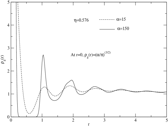
Figure 1: Density $\rho_{g}(r)$ of an amorphous structure calculated from Eq.$(2.5)$ using the data of $g(R)$ found from molecular dynamic simulation of granular particles subjected to a sequence of vertical tapes for $\alpha=150$ (strong localization condition) and $\alpha=15$ (weak localization condition)

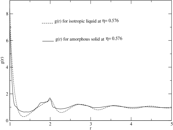
Figure 2: Comparison of pair correlation function $g(R)$ of an amorphous structure and homogeneous liquid at the same packing fraction $\eta=0.576$

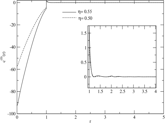
Figure 3: Direct pair correlation function $c^{(0)}(r)$ as a function of distance r at packing fraction $\eta=0.50$ and $0.55$ found from the integral equation theory. The inset shows at the magnified scale the value for $r\geq 1$

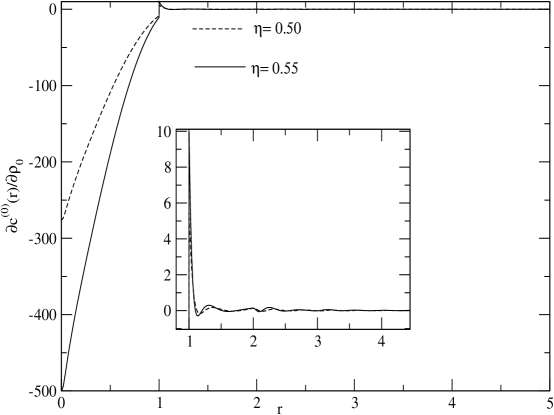
Figure 4: Density derivatives of direct pair correlation function $c^{(0)}(r)$ at $\eta=0.50$ and $0.55$ found from the integral equation theory. The inset shows at magnified scale the value for $r\geq 1$.

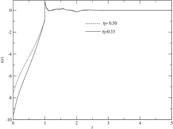
Figure 5: Values of $t(r)$ as a function of distance for $\eta=0.50$ and $\eta=0.55$

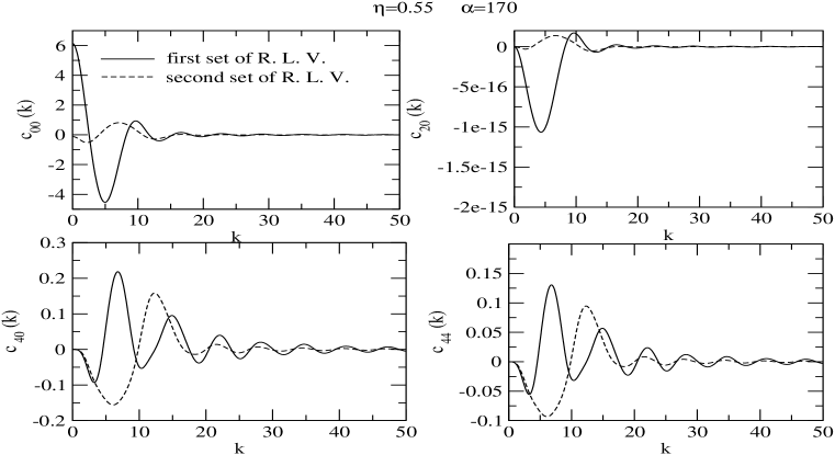
Figure 6: Values of harmonic coefficients ${c^{(G)}}_{lm}(k)$ for first two sets of reciprocal lattice vectors of a f.c.c. crystal for $\eta=0.55$ and $\alpha=170$

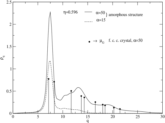
Figure 7: Comparison of order parameters of amorphous structure for $\alpha=50$ and $15$ and of a f.c.c. crystal for $\alpha=50$ at $\eta=0.596$

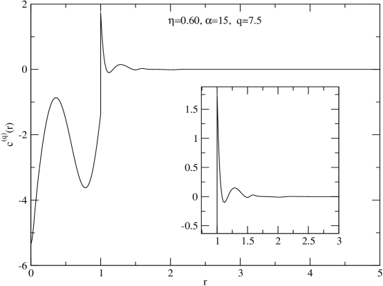
Figure 8: Values of $c^{(q)}(r)$ as a function of distance $r$ at $q=7.53$ at which $\rho_{q}$ is maximum. Inset magnifies the value of $c^{(q)}(r)$ for $r\geq 1$

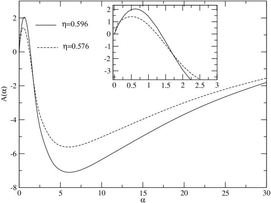
Figure 9: Free energy difference $\Delta A=A[\rho_{0}]-A_{l}[\rho_{0}]$ as a function of localization parameter $\alpha$ at $\eta=0.576$ and $0.596$ for amorphous structures. The inset shows at magnified scale the energy barrier that separates the minimum of amorphous structure from that of homogeneous fluid.

References

- (1) P. M. Chaikin and T. C. Lubensky, Principles of Condensed Matter Physics (Cambridge University Press, 1995)
- (2) M. D. Ediger, C. A. Angell and S. Nagel, J. Phys. Chem. 100, 13200 (1996)
- (3) P. G. Debenedetti and F. H. Stillinger, Nature 410, 259 (2001)
- (4) L. O. Hedges, R. L. Jack, J. P. Garrahan and D. Chandler, Science 323, 1309 (2009)
- (5) A. Cavagna, Phys. Rep. 476, 51 (2009)
- (6) G. Parisi and F. Zamponi, Rev. Mod. Phys. 82, 789(2010)
- (7) W. Kob., C. Donati, S. Plimpton, P. H. Poole and S. C. Glotzer, Phys. Rev. Lett.79, 2827(1997)
- (8) J. P. Hensen and I. R. Mc Donald, Theory of Simple Liquids, 3rd edition (Elsevier, 2006)
- (9) P. Mishra and Y. Singh, Phys. Rev. Lett. 97, 177801 (2006)
- (10) S. L. Singh and Y. Singh, Europhys. Lett. 88, 16005 (2009)
- (11) T. V. Ramakrishanan and M. Yussouff, Phys. Rev. B. 19, 2775 (1979)
- (12) Y. Singh, Phys. Rep. 207, 351 (1991)
- (13) H. Lowen, Phys. Rep. 237, 249(1994)
- (14) A. R. Denton and N. W. Ashcroft, Phys. Rev. A 39, 4701 (1989); A. Khen and N. W. Ashcroft, Phys. Rev. Lett. 78, 3346 (1997)
- (15) J. H. Conway and N. J. A. Sloane, Sphere packings, Lattices and Groups (Springer-Verlag, New York, 1993)
- (16) S. Torquato, T. M. Truskett and P. G. Debenedetti, Phys. Rev. Lett. 84, 2064 (2000)
- (17) C. S. O’Hern, S. A. Langer, A. J. Liu and S. Nagel, Phys. Rev. Lett, 88, 075507 (2002); L. E. Silbert, A. J. Liu and S. R. Nagel, Phys. Rev. E. 73, 041304(2006)
- (18) R. D. Kamien, A. J. Liu, Phys. Rev. Lett. 99, 155501 (2007)
- (19) P. Tarazona, Mol. Phys. 52, 81 (1984)
- (20) A. Donev, F. H. Stilinger and S. Torquato, Phys. Rev. Lett. 96, 225502 (2006), A. Donev, R. Connelly, F. H. Stillinger and S. Torquato, Phys. Rev. E. 75, 051304 (2007)
- (21) M. Pica. Ciamarra, M. Nicodemi and A. Coniglio, Phys. Rev. E 75, 021303(2007)
- (22) F. J. Rogers and D. A. Young, Phys. Rev. A. 30, 999 (1984)
- (23) M. J. Gillan, Mol. Phys. 38, 1781(1979)
- (24) J. L. Barrat, J. P. Hansen and G. Pastore, Mol. Phys., 63, 747(1988), Phys. Rev. Lett. 58, 2075(1987)
- (25) W. G. Hoover and F. H. Ree, J. Chem. Phys. 49, 3609 (1968)
- (26) B. J. Alder, W. G. Hoover and D. A. Young, J. Chem. Phys. 49, 3688(1968)
- (27) D. C. Wang and A. P. Gast, J. Chem. Phys. 110, 2522(1999)
- (28) B. B. Laird, and D. M. Kroll, Phys. Rev. A. 42, 4810(1990)
- (29) J. L. Barrat, J. P. Hansen and G. Pastore and E. M. Waisman, J. Chem. Phys. 86, 6360(1987)
- (30) B. B. Laird, J. D. McCoy and A. D. J. Heymat, J. Chem. Phys. 87, 5449(1987)
- (31) L. Berthier and T. A. Witten, Phys. Rev. E. 80, 021502(2009), Y. Burmer, D. R. Reichmann, Phys. Rev. E. 69, 041202(2004)
- (32) P. Chaudhari, L. Berthier and S. Sastry, Phys. Rev. Lett. 104, 165701(2010)
- (33) C. Bennet, J. Appl. Phys. 43, 2727(1972)
- (34) M. Baus and Jean-Louis Colot, J. Phys. C 19, L135(1986) H. Lowen, J. Phys. Cond Matt 2, 8477(1990)
- (35) Y. Singh, J. P. Stossel and P. G. Wolyness, Phys. Rev. Lett. 54, 1059(1985)
- (36) C. Kaur and S. P. Das, Phys. Rev. Lett. 86, 2062(2001)
- (37) C. Dasgupta, Europhys. Lett. 20, 131(1992); C. Dasgupta and O. T. Valls, Phys. Rev. E. 59, 3123(1999)