Entanglement in the classical limit: quantum correlations from classical probabilities

Abstract

We investigate entanglement for a composite closed system endowed with a scaling property allowing to keep the dynamics invariant while the effective Planck constant $\hslash_{\mathrm{eff}}$ of the system is varied. Entanglement increases as $\hslash_{\mathrm{eff}}\rightarrow 0$. Moreover for sufficiently low $\hslash_{\mathrm{eff}}$ the evolution of the quantum correlations, encapsulated for example in the quantum discord, can be obtained from the mutual information of the corresponding classical system. We show this behavior is due to the local suppression of path interferences in the interaction that generates the entanglement. This behavior should be generic for quantum systems in the classical limit.

Entanglement is a distinctive feature of quantum mechanics, “the one that enforces its entire departure from classical lines of thought” schroedinger . Its understanding has tremendously progressed in the last decade, due essentially to a vast amount of work regarding the construction and properties of entangled qubits in view of possible applications in quantum information horodecki . In a more general context, any dynamical interaction between quantum particles leads to entanglement, that stands as a formidable obstacle to account for the emergence of classical word. Explaining the unobservability of entanglement in the classical limit is one of the aims of the decoherence programme zurek .

Somewhat more modestly, several recent works refQC have studied in semiclassical systems the link between the generation of entanglement and the dynamics of the corresponding classical system, including in experimental realizations exp . The numerical and analytical results obtained so far indicate that the entanglement dynamics in quantum systems having a classically chaotic counterpart sharply differs from those whose classical counterpart is regular, though this difference is dependent on the specificities of the considered systems (types and strengths of the coupling, choice of initial states, etc.). It has been argued argued that a proper understanding of the connection between the classical dynamical regime and entanglement hinges on employing systems in which the same physical process generates the dynamics in the classical system and entanglement in its quantum counterpart.

An intriguing question studied in this paper concerns the behavior of entanglement in these systems when the typical actions of the system grow with respect to $\hslash$. Then the size of the Hilbert space increases and the quantum-classical correspondence improves. Moreover if the system dynamics can be kept invariant while the actions increase, an effective Planck constant $\hslash_{\mathrm{eff}}$ can be defined and entanglement can be studied as $\hslash_{\mathrm{eff}}\rightarrow 0$. We will see that entanglement indeed increases with the size of the Hilbert space in agreement with previous findings on entangled Bose-Einstein condensates angelo . Maybe more surprisingly for sufficiently low $\hslash_{\mathrm{eff}}$ the evolution of the entanglement measure is given by probabilities obtained from the classical dynamical evolution, irrespective of the dynamical regime. A consequence discussed below is whether in the $\hslash_{\mathrm{eff}}\rightarrow 0$ limit the quantum information encoded in the pure state density matrix becomes indiscernible from the classical information contained in a mixed density matrix yielding the same reduced dynamics.

Let us consider bipartite entanglement generated by repeated inelastic scattering of two particles. To set the model, let us assume a light structureless particle and a heavy rotating particle, modeled by a symmetric top with angular momentum $N$ and energy $E_{N}=N(N+1)/2I$, $I$ denoting the moment of inertia. The scattering potential is taken to be a contact interaction so that the light incoming particle receives a kick when it hits the rotating top. The conservation of the total angular momentum $\mathbf{T}=\mathbf{N}+\mathbf{J}$ where $J$ is the light particle angular momentum, imposes that after the collision the rotating top is left with an angular momentum $N^{\prime}$ obeying $T-J\leq N^{\prime}\leq T+J$ where we have assumed $J^{\prime}=J$. The probability of the transition $N\rightarrow N^{\prime}$ is obtained from the scattering matrix elements $\left|S_{NN^{\prime}}\right|^{2}$. Finally to account for repeated scattering we need an attractive long-range field between both particles: we will assume the particles have opposite electric charge. Note that this model can be seen as a two-particle extension of the standard kicked top well-known in quantum chaos exp ; haake .

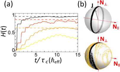
Figure 1: (a) The entanglement rate as a function of the number of kicks is given for quantum systems characterized by $k=0.25$ and $\hbar_{\mathrm{eff}}=0.5,0.25,0.1,0.01$ (from bottom to top). The dashed lines result from applying the scaling relation (4) to the 3 upper curves. (b) Top: The black ring encircling the $\mathbf{N}$ axis is the initial classical distribution of $\mathbf{J}$ with $J=10$ (corresponding to the quantum case with $\hbar_{\mathrm{eff}}=0.1$), centered on $N_{0}=T=50$. Bottom: The distribution at $t=10$ kicks (black dots), showing a spread. The surface of section for $k=0.25$ is shown in yellow (light gray).

Starting from an initial product state $\left|\psi_{0}\right\rangle\equiv\left|F_{0}^{-}(\bar{\epsilon}_{0})\right\rangle\left|N_{0}\right\rangle$ where $\left|F_{0}^{-}\right\rangle$ depicts an incoming wavepacket of the light particle with mean energy $\bar{\epsilon}_{0}$ traveling towards the rotating top in state $\left|N_{0}\right\rangle,$ entanglement is generated as soon as the first collision takes place. The outgoing wavefunction is then given by the superposition $\sum_{N}S_{NN_{0}}\left|F^{+}(\epsilon_{N})\right\rangle\left|N\right\rangle$ where the dependence of $\epsilon$ on $N$ is due to the conservation of energy, $\epsilon_{N}=E-E_{N}$, with $E=\bar{\epsilon}_{0}+E_{N_{0}}$ being the total energy. The scattered wavepackets are later turned back by the attractive field and are treated as newly incoming waves. The pure state density matrix

$$\rho(t)=U(t,t_{0})\left|\psi_{0}\right\rangle\left\langle\psi_{0}\right|U^{+}(t,t_{0})$$ (1)

is obtained by writing the evolution operator $U$ in terms of the scattering eigenstates of the Hamiltonian

$$\left|\psi(E)\right\rangle = \sum_{N}Z_{N}^{-}(E)\left|F^{-}(\epsilon_{N})\right\rangle\left|N\right\rangle+\sum_{NN^{\prime}}$$ (2)

$$Z_{N}^{-}(E)S_{N^{\prime}N}\left|F^{+}(\epsilon_{N^{\prime}})\right\rangle\left|N^{\prime}\right\rangle$$

where $Z_{N}^{-}$ are coefficients obtained by applying the asymptotic boundary conditions. The maximal number of entangled states is given by the number of scattering channels $n=2J+1$. The amount of entanglement will be estimated through the entropy of the reduced density matrix. We will employ the linearized form

$$H(t)=\frac{n}{n-1}\left(1-\mathrm{Tr}_{N}\rho_{N}^{2}(t)\right)$$ (3)

that becomes a good approximation for large $n$. $\rho_{N}(t)$ is the reduced density matrix obtained by tracing over the light particle’s degrees of freedom. Note $H=1$ for a maximally entangled state. For convenience we set from now on $t_{0}=\tau_{\epsilon}/2$ where $\tau_{\epsilon}$ is the period of the mean energy orbit; then the collision times are $t=q\tau_{\epsilon}$ with $q$ being an integer.

The classical version of the model can be formally obtained by employing the semiclassical link lombardi04 between the deflection angle $\phi$ produced by the torsional motion and the eigen-phaseshifts $\delta$ of the $S$-matrix: in the top’s reference frame, each kick rotates $\mathbf{J}$ by an angle $\phi=kJ_{\bot}/J=\partial\delta/\partial J_{\bot}$ where $J_{\bot}$ is the projection of $\mathbf{J}$ on the unit axis $\mathbf{\hat{N}}_{\bot}$ perpendicular to $\mathbf{N}$. $k$ is the strength of the kick; a given $k$ corresponds, via the semiclassical relation, to a given $S$-matrix, i.e. $S_{NN^{\prime}}=S_{NN^{\prime}}(k)$. The classical orbit of the light particle between two scattering events induces a rotation of $\mathbf{J}$ around $\mathbf{N}$ by an angle $2\pi\tau_{\epsilon}/\tau_{N}$ where $\tau_{N}$ is the top rotation period. A surface of section is obtained by plotting the position of $\mathbf{J}$ after each kick (see Figs 1(b) and 3). The crucial observation is that the surface of section only depends on $k$ and on $\tau_{\epsilon}/\tau_{N}$: $N,J$ and $T$ (which are action variables) can be increased at will, say by division by $\hslash_{\mathrm{eff}},$ but the dynamical map stays constant provided $E$ and $I$ are adjusted accordingly. For a long-range central field this also implies dividing the radial action $W_{r}$ of the light particle by the same constant $\hslash_{\mathrm{eff}}.$ Hence multiplying $N,J,T$ and $W_{r}$ by the common factor $1/\hslash_{\mathrm{eff}}\gg 1$ is tantamount to studying the limit $\hslash\rightarrow 0$ without modifying the underlying dynamics. Note that the number of entangled states $n$ also scales with $1/\hslash_{\mathrm{eff}}.$

Fig. 1(a) displays the entanglement evolution for the quantum two-particle kicked top with $k=0.25$ for different values of $\hslash_{\mathrm{eff}}$ (we employ atomic units and set $\hbar=1$). The light particle’s initial distribution is a Gaussian wavepacket localized far from the symmetric top with its mean initial momentum directed towards it. The entanglement increases dramatically as $\hslash_{\mathrm{eff}}$ decreases, despite the fact that the initial state takes a smaller relative area on the sphere. To first order, this is a consequence of the similarity transformation: on the one hand $\rho_{N}(t)$ is by definition a convex combination of projectors $\left|N\right\rangle\left\langle N\right|$, and on the other hand in the semiclassical approximation the projection of $\rho_{N}(t)$ on the unit sphere (at kick times $t=q\tau_{\epsilon})$ covers the same area irrespective of $\hslash_{\mathrm{eff}}$. Let $m$ be the number of projectors $\left|N\right\rangle\left\langle N\right|$ (out of total of $n$) projecting in this area for some $\hslash_{\mathrm{eff}}$ and $m^{\prime}$ that number for another choice of $\hslash_{\mathrm{eff}}^{{}^{\prime}}<\hslash_{\mathrm{eff}}$. Then $m/n=m^{\prime}/n^{\prime}$ from which it follows that for situations corresponding to the maximal entanglement (uniform distribution in that region) there is a simple scaling relation for the purity $1-H$ yielding

$$H^{\prime}(t)=1-\frac{\hslash_{\mathrm{eff}}^{\prime}}{\hslash_{\mathrm{eff}}}\left(1-H(t)\right).$$ (4)

As expected entanglement increases with the number of available quantum states.

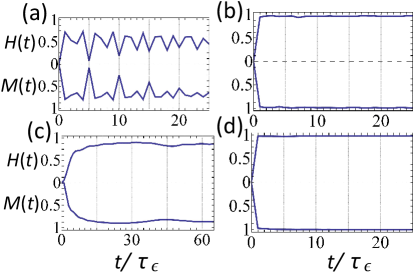
Figure 2: Each panel shows the entanglement evolution as computed from the entropy $H(t)$ (top curve), along with the mutual information $M(t)$ of the classical counterpart (upside-down curve), where $t$ is computed at the discrete kick times $t=q\tau_{\epsilon}$. The parameters are $J=100,T=500$ (corresponding to $\hbar_{\mathrm{eff}}=0.01$ for the quantum system) and (a): $k=1,N_{0}=402$, (b): $k=1,N_{0}=430$, (c): $k=0.01,N_{0}=498$, (d): $k=10,N_{0}=460$.

The classical evolution analogue of the quantum problem leading to Fig. 1(a) is obtained by taking an initial uniform distribution of angular momentum $N_{0}-\frac{1}{2n}<N<N_{0}+\frac{1}{2n}$, i.e. we cut the sphere along the $\mathbf{N}$ axis into $n$ slices of width $1/n$. Each slice is centered so that the projection $J_{\parallel}$ on the $\mathbf{\hat{N}}_{\parallel}$ axis matches integer values of $N$. Thus the initial classical distribution corresponding to $\left|N_{0}\right\rangle\left\langle N_{0}\right|$, is represented on the sphere by the ring centered at $J_{\parallel}(N_{0})=\mathbf{T}\cdot\mathbf{\hat{N}}_{\parallel}-N_{0}$. The light particle initial distribution is the same Gaussian employed in the quantum problem (the role of this distribution is to give a statistical weight, depending on the initial energy of the light particle, to each $\mathbf{J}$ lying in the initial ring). We compute numerically the evolution (torsion during the kick and rotation during the orbital excursion) for each $\mathbf{J}$ of the initial distribution from kick to kick. The classical probability $p_{N}^{cl}(t=q\tau_{\epsilon})$ of finding the top with an angular momentum in the interval $\Delta_{N}=[N-\frac{1}{2n},N+\frac{1}{2n}]$ after $q$ kicks is obtained by counting the vectors $\mathbf{J}$ whose projection falls in the corresponding interval. The probabilities after the first kick are given by the transition probability $P^{cl}(\Delta_{N_{0}}\rightarrow\Delta_{N})$. The classical probabilities after $q$ kicks obey the recurrence relation

$$p_{N}^{cl}(q\tau_{\epsilon})=\sum_{N^{\prime}}P^{cl}(\Delta_{N^{\prime}}\rightarrow\Delta_{N})p_{N^{\prime}}^{cl}\left[\left(q-1\right)\tau_{\epsilon}\right].$$ (5)

From these probabilities one can define the quantity

$$M(q\tau_{\epsilon})=\frac{n}{n-1}\left(1-\sum_{N}\left[p_{N}^{cl}(q\tau_{\epsilon})\right]^{2}\right)$$ (6)

that can be understood equivalently as the linear entropy for the total system or as the (linearized) classical mutual information , quantifying the amount of mixing among the $n$ slices induced by the kicks.

Fig. 2(a)-(d) shows in the top panel the entanglement evolution as given by $H(t=q\tau_{\epsilon})$ for a choice of system parameters (coupling $k$ and initial state) all corresponding to $\hslash_{\mathrm{eff}}\approx 1/100$, two orders of magnitude smaller than the hard quantum case $\hslash_{\mathrm{eff}}\approx 1$ (which is the typical value for qubits), but still considerably larger than typical values characterizing classical actions. The bottom panel in each plot shows $M(q\tau_{\epsilon})$ obtained from the classical probabilities through Eq. (6). The good agreement between $H(t)$ and the time-dependent classical probabilities holds for classically chaotic and regular regimes alike as can be inferred from Fig. 3, displaying the corresponding surfaces of section along with the classical distributions whose spread along the $\mathbf{N}_{\parallel}$ axis accounts for the entanglement evolution.

Although quantifying entanglement by means of classical probabilities might appear surprising at first sight, we expect this behavior to be generic for semiclassical systems that undergo a loss of phase coherence. This is indeed the first ingredient by which the classical $M(q\tau_{\epsilon})$ can account for $H(t)$. The second ingredient is the semiclassical approximation itself that allows to express operator matrix elements in terms of classical quantities (the action and the density of paths). For the system under consideration we start by writing Eq. (2) in the form $\left|\psi(E)\right\rangle=\sum_{N}B_{N}(E)\left|F(\epsilon_{N})\right\rangle\left|N\right\rangle$ where $\left|F\right\rangle$ is a standing wave obtained by combining the $\left|F^{\pm}\right\rangle$ and $B_{N}(E)\equiv\sum_{N^{\prime}}S_{NN^{\prime}}Z_{N^{\prime}}^{-}(E)e^{i(W_{r}^{po}(\epsilon_{N})-\pi)/2};W_{r}^{po}$ is the radial action of the classical periodic orbit in the attractive field. Then Eq. (1) takes the form

$$\rho(t = q\tau_{\epsilon})=\sum_{NN^{\prime}}\left|N\right\rangle\left\langle N^{\prime}\right|e^{-i(E_{N}-E_{N^{\prime}})t}$$ (7)

$$\beta_{N}(t)\beta_{N^{\prime}}^{\ast}(t)\left|F(\bar{\epsilon}_{N})\right\rangle\left\langle F(\bar{\epsilon}_{N^{\prime}})\right|$$

with

$$\beta_{N}(t) = \sum_{N^{\prime}}S_{NN^{\prime}}\left[\sum_{E}e^{-i\epsilon_{N}t}Z_{N^{\prime}}^{-}(E)\left\langle\psi(E)\right|\left.\psi_{0}\right\rangle\right]$$ (8)

$$e^{i(W_{r}^{po}(\epsilon_{N})-\pi)/2}$$

(keep in mind $\epsilon_{N}=E-E_{N}$ when taking the sum). The reduced density matrix is readily derived as $\rho_{N}(t=q\tau_{\epsilon})=\sum_{N}\left|N\right\rangle\left\langle N\right|p_{N}(t)$ with

$$p_{N}(t=q\tau_{\epsilon})=\left|\beta_{N}(t+\frac{\tau_{\epsilon}}{2})\right|^{2}=\left|\sum_{N^{\prime}}S_{NN^{\prime}}\zeta_{N^{\prime}}^{-}(t)\right|^{2}.$$ (9)

$\zeta_{N^{\prime}}^{-}(t)$ is defined by the term between $[..]$ in Eq. (8) (i.e. by excluding the phase term in the sum). $\left|\zeta_{N^{\prime}}^{-}(t)\right|^{2}$ represents the probability on the incoming channel $N^{\prime}$ just before the collision, whereas $\left|\sum_{N^{\prime}}S_{NN^{\prime}}\zeta_{N^{\prime}}^{-}\right|^{2}$ is the weight of the outgoing wave right after the collision ($t=q\tau_{\epsilon}$); in the semiclassical limit this is the same as the weight $\left|\beta_{N}\right|^{2}$ at the apogee half a period later . It follows that $\zeta_{N}^{-}(q\tau_{\epsilon})=p_{N}\left[\left(q-1\right)\tau_{\epsilon}\right].$ Finally we recall lombardi04 that in the semiclassical regime the $S$-matrix elements are given to first order in $\hslash$ by

$$S_{NN^{\prime}}=\mathcal{A}_{NN^{\prime}}e^{i\mathcal{S}_{NN^{\prime}}/\hslash}\text{ with }\left|\mathcal{A}_{NN^{\prime}}\right|^{2}=P^{cl}(\Delta_{N^{\prime}}\rightarrow\Delta_{N})$$ (10)

and $\mathcal{S}_{NN^{\prime}}$ is the classical action (the boundary conditions for the conjugate momenta obey $p_{\theta}(t\rightarrow-\infty)=N^{\prime}$ $p_{\theta}(t\rightarrow+\infty)=N$). As $\mathcal{S}_{NN^{\prime}}/\hslash\rightarrow\infty$ the phase terms $\exp i(\mathcal{S}_{NN_{1}}-\mathcal{S}_{NN_{2}})/\hslash$ in Eq. (9) oscillate wildly, while the amplitudes $\mathcal{A}_{NN^{\prime}}$ are of the same order of magnitude. As a result these off-diagonal terms are suppressed, so we may keep only the terms with $N_{1}=N_{2}$. Eq. (9) becomes

$$p_{N}(t=q\tau_{\epsilon})=\sum_{N^{\prime}}P^{cl}(\Delta_{N^{\prime}}\rightarrow\Delta_{N})p_{N^{\prime}}\left[\left(q-1\right)\tau_{\epsilon}\right].$$ (11)

Comparing with Eq. (5) and given that the initial conditions are identical in the quantum and classical problems, we see that provided the approximations employed hold, the entanglement entropy $H(t=q\tau_{\epsilon})$ becomes identical to the mutual information $M(q\tau_{\epsilon})$ of the corresponding classical system given by Eq. (6), thereby explaining the numerical results displayed in Fig. 2.

A remarkable consequence of the present results concerns the classical values taken by quantifiers of quantum correlations. For example the quantum discord $D(\rho)$ zurek01 widely employed in the context of qubit density matrices, measures the quantum information that can only be extracted by joint measurements on both subsystems. $D(\rho)$ vanishes if the state has only classical correlations. Here $D(\rho)$ is simply given by $H(t),$ hence by the classical mutual information $M(t)$. Put differently, the quantum information contained in the entangled state – which would be the information gained by an observer making a measurement (for example measuring the light particle’s energy $\epsilon_{N_{m}}$ projects the top to the rotational state $\left|N_{m}\right\rangle$) – is given by the ignorance spread arising from the dynamical evolution of the corresponding classical system.

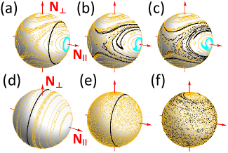
Figure 3: Classical evolution and surfaces of section for the parameters corresponding to the plots of Fig. 2. (a)-(c): for $k=1$ (mixed phase-space), (a) gives the initial distributions for $N_{0}=402$ (blue [grey] ring) and $N_{0}=430$ (black ring); (b) displays the distributions after 10 kicks, (c) at $t=25$. (d): position of the initial distribution defined by $N_{0}=498$ for $k=0.01$ (regular dynamics). (e)-(f): Distributions for $k=10$ (mostly chaotic phase-space) and $N_{0}=460$ at $t=0$ [(e)] and at $t=5$ kicks [(f)].

The conjunction of ubiquitous entanglement as the classical limit is approached, and the role played by classical probabilities to account for quantum correlations in that limit allows us to speculate whether from a statistical perspective, entanglement may be converted within the closed system into classical correlations, without the need to invoke couplings with an additional system (e.g. an environment). Indeed $\rho(t)$ cannot operationally be distinguished from the density matrix $\rho^{cc}(t)=\sum p_{N}^{cl}\left|N\right\rangle\left\langle N\right|\left|F(\bar{\epsilon}_{N})\right\rangle\left\langle F(\bar{\epsilon}_{N})\right|$ containing only classical correlations (and for which $D(\rho^{cc})=0$): the reduced density matrices obtained from $\rho$ and $\rho^{cc}$ are identical, and as $\hslash\rightarrow 0$ the coherences (in the “pointer basis”$\left|F(\bar{\epsilon}_{N})\right\rangle\left|N\right\rangle$) of typical two-particle observables would lead to interference patterns with vanishing (and therefore undetectable) wavelengths ballentine .

To sum up, we have investigated entanglement evolution when the entanglement is generated by a dynamical localized interaction in a quantum system having a well defined classical counterpart. We have seen that entanglement increases, irrespective of whether the underlying dynamics is regular or chaotic, as typical actions grow relative to $\hbar$. The quantum correlations are then given by the mutual information of the corresponding classical system. The present results could contribute to a better understanding of the role played by quantum information in the classical limit.

References

- (1) E. Schroedinger, Proc. Cam. Phil. Soc. 31, 555 (1935).
- (2) R. Horodecki et al, Rev. Mod. Phys. 81, 865 (2009).
- (3) W. H. Zurek, Rev. Mod. Phys. 75, 715 (2003).
- (4) K. Furuya et al., Phys. Rev. Lett. 80, 5524 (1998); J.N Bandyopadhyay and A. Lakshminarayan, Phys. Rev. Lett. 89, 060402 (2002); M. Znidaric and T. Prosen, J. Phys. A 36, 2463 (2003); Ph. Jacquod, Phys. Rev. Lett. 92 , 150403 (2004); M. Lombardi and A. Matzkin, Europhys. Lett. 74, 771 (2006); A.M. Ozorio de Almeida, Lect. Notes Phys. 768, 157 (2009).
- (5) S. Chaudhury et al., Nature 461, 768 (2009).
- (6) M. Lombardi and A. Matzkin, Phys. Rev. A 73, 062335 (2006); C. M. Trail et al, Phys. Rev. E 78, 046211 (2008).
- (7) R. M. Angelo and K. Furuya, Phys. Rev. A 71, 042321 (2005).
- (8) F. Haake, Quantum Signatures of Chaos (Springer, Berlin, 2004).
- (9) W.H. Miller, Adv. Chem. Phys. 25, 69 (1974). B. Dietz et al., Ann. Phys. 312, 441 (2004).
- (10) H. Ollivier and W. H. Zurek, Phys. Rev. Lett. 88, 017901 (2001).
- (11) L. E. Ballentine Phys. Rev. A 70, 032111 (2004); M. Castagnino et al Class. Quantum. Grav. 25 154002 (2008).