The spin anisotropy of the magnetic excitations in the normal and superconducting states of optimally doped YBa₂Cu₃O_6.9 studied by polarized neutron spectroscopy

Abstract

We use inelastic neutron scattering with spin polarization analysis to study the magnetic excitations in the normal and superconducting states of YBa₂Cu₃O_6.9. Polarization analysis allows us to determine the spin polarization of the magnetic excitations and to separate them from phonon scattering. In the normal state, we find unambiguous evidence of magnetic excitations over the 10–60 meV range of the experiment with little polarization dependence to the excitations. In the superconducting state, the magnetic response is enhanced near the “resonance energy” and above. At lower energies, 10$\lesssim$$E$$\lesssim$30 meV, the local susceptibility becomes anisotropic, with the excitations polarized along the c-axis being suppressed. We find evidence for a new diffuse anisotropic response polarized perpendicular to the $c$-axis which may carry significant spectral weight.

I Introduction

High temperature superconductivity (HTS) arises when certain two dimensional antiferromagnetic Mott insulators are electron or hole doped HTC . The antiferromagnetic parent compounds such as La₂CuO₄ show spin-wave excitations up to $2J$$\approx$300 meV Headings et al. (2010). Doping causes the magnetic response to evolve from that of spin waves to a more structured response Cheong et al. (1991); Rossat-Mignod et al. (1991); Mook et al. (1993); Fong et al. (1995); Bourges et al. (1997); Mook et al. (1998); Dai et al. (1999); Hayden et al. (2004); Vignolle et al. (2007); Fauqué et al. (2007); Xu et al. (2009), with strong spin fluctuations being observed for superconducting compositions in a number of systems including YBa₂Cu₃O_6+x (YBCO) Mook et al. (1998); Bourges et al. (1997); Dai et al. (1999); Hayden et al. (2004); Stock et al. (2005); Woo et al. (2006), La_2-xSr_xCuO₄ Hayden et al. (1996); Vignolle et al. (2007) and Bi₂Sr₂CaCu₂O_8+δ Fong et al. (1999); Fauqué et al. (2007); Xu et al. (2009). Many optimally-doped cuprates show a strong well-defined collective magnetic excitation which is localised in reciprocal space and strongest near the $\mathbf{Q}$=(1/2,1/2)$\equiv$($\pi,\pi$) position. It is sharp in energy and develops on cooling through the critical temperature. This excitation has become known as the “magnetic resonance”. The magnetic resonance has been observed in YBa₂Cu₃O_6+x Rossat-Mignod et al. (1991); Mook et al. (1993); Fong et al. (1995), Bi₂Sr₂CaCu₂O_8+δ Fong et al. (1999), Tl₂Ba₂CuO_6+δ He et al. (2002) and HgBa₂CuO_4+δ Yu et al. (2010).

The magnetic resonance is certainly the strongest feature in the magnetic excitations spectrum of the materials listed above, however, it only accounts for a small faction ($\approx$2%) Dai et al. (1999); Fong et al. (1999); Woo et al. (2006) of the total scattering expected from the unpaired 3$d$ electrons of the Cu atoms. In this work we search for other contributions to the response which are spread out in energy and wavevector but nevertheless may carry significant spectral weight. These are harder to observe because they are weak and may not show the strong temperature dependence which allows the resonance to be easily isolated. We use inelastic neutron scattering with polarization analysis to isolate the magnetic scattering from phonon scattering.

We find that there is a significant response in the normal state which can account for much of the spectral weight from which the resonance is formed. In the superconducting state, we find evidence for a diffuse contribution at energies well below the resonance. This new contribution is polarized with strong fluctuations perpendicular to the $c$-axis.

II Background

II.1 Polarization Analysis

Neutrons scatter from condensed matter via two processes: (i) The electromagnetic interaction probes fluctuations in the magnetization density of the electrons (in this paper this is referred to as magnetic scattering). (ii) The strong nuclear force is responsible for scattering from the atomic nuclei. The nuclear scattering allows us to probe phonons which are correlations (in time and space) between the position of the nuclei. The existence of two distinct scattering processes makes the neutron an extremely versatile probe. However, it also means that the two types of scattering can mask each other.

Polarization analysis of the neutron’s spin allows the separation of magnetic and nuclear (phonon) scattering. In the present work, we use longitudinal polarization analysis (LPA). In LPA, a spin-polarized incident neutron beam is created and its polarization maintained by a small magnetic field ($\sim$1 mT). The number of neutrons scattered with spins parallel or antiparallel to this quantizing field are then measured. We label each spin-polarization state as parallel ($\equiv$up,$\uparrow$,+) or antiparallel ($\equiv$down,$\downarrow$,$-$) to the applied field. The cross sections are referred to as spin-flip (SF) ($\uparrow\rightarrow\downarrow$,$\downarrow\rightarrow\uparrow$) or non-spin-flip (NSF) ($\uparrow\rightarrow\uparrow$,$\downarrow\rightarrow\downarrow$). A natural reference frame in which to understand the cross sections is one referenced to the scattering vector $\mathbf{Q}=\mathbf{k}_{i}-\mathbf{k}_{f}$ of the neutron, where $\mathbf{k}_{i}$ and $\mathbf{k}_{f}$ are the incident and final wavevectors of the neutron. Thus, $\mathbf{\hat{x}}\parallel\mathbf{Q}$, $\mathbf{\hat{y}}\perp\mathbf{Q}$, and $\mathbf{\hat{z}}\perp\mathbf{Q}$ and $\perp$ to the spectrometer scattering plane (the plane containing $\mathbf{k}_{i}$ and $\mathbf{k}_{f}$). We make measurements with the neutrons polarized along each of these axes.

The neutron cross sections as a function of spin polarization have been derived and presented elsewhere Blume (1963); Maleyev et al. (1963); Moon et al. (1969); Squires (1978); Lorenzo et al. (2007). The spin-flip magnetic cross section for spin polarization $\parallel\mathbf{Q}$ is

$$\sigma_{xx}^{\uparrow\downarrow}=\left(\frac{d^{2}\sigma}{d\Omega dE}\right)_{\mathbf{H}\parallel x}^{\uparrow\rightarrow\downarrow} = \frac{k_{f}}{k_{i}}\frac{(\gamma r_{e})^{2}}{g^{2}\mu^{2}_{B}}\frac{1}{\pi}F^{2}(\mathbf{Q})$$ (1)

$$\times \frac{\chi_{yy}^{\prime\prime}({\bf q},\hbar\omega)+\chi_{zz}^{\prime\prime}({\bf q},\hbar\omega)}{1-\exp(-\hbar\omega/kT)},$$

where $(\gamma r_{\text{e}})^{2}$=0.2905 barn sr^-1 and $|F({\bf Q})|^{2}$ is the anisotropic magnetic form factor for a Cu²⁺ $d_{x^{\scriptstyle 2}-y^{\scriptstyle 2}}$ orbital. $\chi_{\nu\nu}^{\prime\prime}({\bf q},\hbar\omega)$ is the generalized susceptibility corresponding to magnetic fluctuations along the $\nu$-axis. Thus, for example:

$$\langle m_{x}^{2}({\bf q},\omega)\rangle=\frac{1}{\pi}\frac{\chi_{xx}^{\prime\prime}({\bf q},\omega)}{1-\exp(-\hbar\omega/kT)},$$ (2)

where the angle brackets denote thermal averages. The spin-dependent cross sections including the nuclear coherent cross sections (i.e. the phonon cross section) $N(\mathbf{q},\omega)$ are:

$$\sigma_{xx}^{\uparrow\downarrow} \propto \chi_{yy}^{\prime\prime}(\mathbf{q},\omega)+\chi_{zz}^{\prime\prime}(\mathbf{q},\omega)+\mathrm{BG}_{\uparrow\downarrow}$$

$$\sigma_{yy}^{\uparrow\downarrow} \propto \chi_{zz}^{\prime\prime}(\mathbf{q},\omega)+\mathrm{BG}_{\uparrow\downarrow}$$

$$\sigma_{zz}^{\uparrow\downarrow} \propto \chi_{yy}^{\prime\prime}(\mathbf{q},\omega)+\mathrm{BG}_{\uparrow\downarrow}$$

$$\sigma_{xx}^{\uparrow\uparrow} \propto N(\mathbf{q},\omega)+\mathrm{BG}_{\uparrow\uparrow}$$

$$\sigma_{yy}^{\uparrow\uparrow} \propto \chi_{yy}^{\prime\prime}(\mathbf{q},\omega)+N(\mathbf{q},\omega)+\mathrm{BG}_{\uparrow\uparrow}$$

$$\sigma_{zz}^{\uparrow\uparrow} \propto \chi_{zz}^{\prime\prime}(\mathbf{q},\omega)+N(\mathbf{q},\omega)+\mathrm{BG}_{\uparrow\uparrow},$$ (3)

where we have neglected the nuclear spin incoherent cross-section which is small in the present experiments Cro and BG denotes the background for the configuration. In this work we isolate two components of the susceptibility by comparing different SF cross sections:

$$\sigma_{xx}^{\uparrow\downarrow}-\sigma_{yy}^{\uparrow\downarrow} \propto \chi_{yy}^{\prime\prime}(\mathbf{q},\omega)$$

$$\sigma_{xx}^{\uparrow\downarrow}-\sigma_{zz}^{\uparrow\downarrow} \propto \chi_{zz}^{\prime\prime}(\mathbf{q},\omega)$$ (4)

II.2 Bilayer Effects

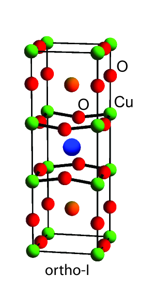
Figure 1: (Color online) The ortho-I structure of YBa₂Cu₃O_6.9.

YBa₂Cu₃O_6+x has two CuO₂ planes per unit cell (See Fig. 1). The usual starting point for models of the magnetic response is to neglect the electronic coupling between CuO₂ planes in different unit cells and include only coupling between the CuO₂ planes of the bilayer located in the center of the unit cell in Fig. 1. This leads to a pair of bonding (b) and antibonding (a) energy bands. The presence of a mirror plane between the two planes of the bilayer means that the magnetic excitations have distinct odd (o) or even (e) character. In this description, the magnetic response is of the form Bulut and Scalapino (1996); Millis and Monien (1996); Brinckmann and Lee (2001); Eremin et al. (2007)

$$\chi^{\prime\prime}(h,k,l,\omega) = \chi_{e}^{\prime\prime}(h,k,\omega)\cos^{2}\left(\frac{\pi d}{c}l\right)$$ (5)

$$+ \chi_{o}^{\prime\prime}(h,k,\omega)\sin^{2}\left(\frac{\pi d}{c}l\right),$$

where $d$ is the separation of the CuO₂ planes. For YBa₂Cu₃O_6.9 $d$=3.38 Å, this means the odd response is strongest at $l$$=$$(n+1/2)c/(2d)$=1.73, 5.3,$\ldots$ The strongest features in the magnetic response of YBa₂Cu₃O_6+x observed by INS are in the odd channel Rossat-Mignod et al. (1991); Mook et al. (1993); Fong et al. (1995) and we measure the odd channel in the present experiment. We note that weaker resonance features have been reported in the even channel Pailhès et al. (2004, 2006) for various dopings. The reported even resonance occurs at higher energy than in the odd channel.

II.3 Sample Details

We investigated a near optimally doped sample of YBa₂Cu₃O_6.9 ($T_{c}$=93 K) grown by a top seed melt growth technique Babu et al. (2000). YBa₂Cu₃O_6.9 has the ortho-I structure show in Fig. 1 with lattice parameters $a$=3.82 Å, $b$=3.89 Å and $c$=11.68 Å ($T$=77 K) Jorgensen et al. (1990). The single crystal studied in the present experiment is twinned and the results presented are an average over the two twin domains. The crystal had a mass of 32.5 g and mosaic spread 1.3^∘. It was annealed for 17 days at 550^∘C, followed by 13 days at 525${}^{\circ}\mathrm{C}$, in oxygen to achieve the required oxygen stoichiometry. Neutron depolarization measurements (see Fig. 4) indicated that $T_{c}(\mathrm{onset})=93$$\pm$0.2 K. Based on $T_{c}$ and the heat treatment Meuffels et al. (1989); Liang et al. (2006), we estimate the oxygen stoichiometry to be $x$=0.9$\pm$0.01.

II.4 Experimental Setup

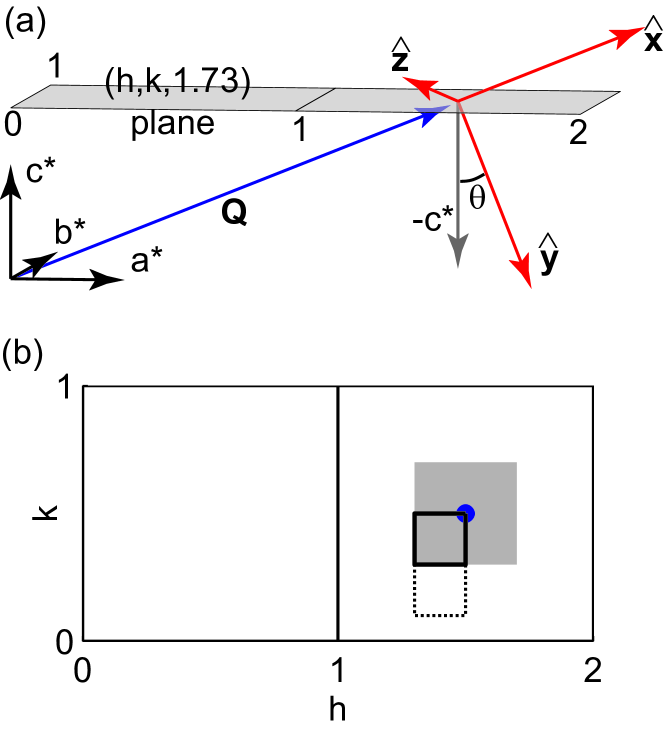
Figure 2: (Color online)(a) Illustration of the reference frame used to describe polarization analysis. Neutrons are polarized along the $\hat{\mathbf{x}}$, $\hat{\mathbf{y}}$ or $\hat{\mathbf{z}}$ axes. $\hat{\mathbf{x}}$ is parallel to $\mathbf{Q}$, $\hat{\mathbf{z}}$ is perpendicular to $\hat{\mathbf{x}}$ and in the $(h,k,0)$ plane. Thus $\hat{\mathbf{x}}\parallel(1.5\mathbf{a}^{\star}$+$0.5\mathbf{b}^{\star}$+$1.8\mathbf{c}^{\star})$, $\hat{\mathbf{y}}\parallel(0.54\mathbf{a}^{\star}$+$0.18\mathbf{b}^{\star}$$-$$4.6\mathbf{c}^{\star})$, $\hat{\mathbf{z}}\parallel(-0.5\mathbf{a}^{\star}$+$1.5\mathbf{b}^{\star})$, $\theta=20.6^{\circ}$ and $\cos^{2}\theta=0.88$. (b) Illustration of the area in reciprocal space where the measurements in Sec. III.2 were made. For $E<52$ meV, we used data collected over the black square (1.3$\leq$$h$$\leq$1.5 and 0.3$\leq$$k$$\leq$0.5) to infer $\chi^{\prime\prime}(\omega)$ measured over the grey area. Data in Fig. 6 covers the black square plus dotted area.

Experiments were performed using the IN20 three-axis spectrometer at the Institut Laue-Langevin, Grenoble using a standard longitudinal polarization analysis set up. Neutron polarization analysis was carried out using a focussing Heusler monochromator and analyzer. The sample was mounted with the [310] and [001] directions in the horizontal scattering plane of the instrument. We worked around the (1.5,0.5,1.73) reciprocal space position so as to avoid strong phonon scattering near $E\approx$40 meV Fong et al. (1995). We used a sample goniometer to access reciprocal space positions out of the $(3h,h,l)$ plane. Data were converted to an absolute scale using a vanadium standard and Eq. 1 and measurement of an acoustic phonon at $\mathbf{Q}$=(0.2,0.2,6). The overall error in the absolute scale is about 20%. We use the reciprocal space of the average tetragonal lattice (with $a\approx 3.86$ Å) to label wavevectors with $\mathbf{Q}=h\mathbf{a}^{\star}+k\mathbf{b}^{\star}+l\mathbf{c}^{\star}$.

In order to reduce neutron depolarization for measurements made in the superconducting state, the sample was cooled through $T_{c}$ and to 10 K while shielded by a $\mu$-metal shield such that $\mu_{0}H<$0.3 $\mu$T. During the measurement, fields in the range $|\mu_{0}\mathbf{H}|$ =0.7-0.11 mT $\ll$ $\mu_{0}H_{c1}$$\approx$25-85 mT were applied to the sample. Therefore, the sample was in the Meissner state.

The finite polarization of the incident neutron beam and other instrumental imperfections leads to a mixing of the spin-flip and non spin-flip channels. This can be described by a flipping ratio $F$, where the measured cross section is:

$$\sigma_{\mathrm{SF}}^{\mathrm{meas}}=\left(\frac{F}{F+1}\right)\sigma_{\mathrm{SF}}+\left(\frac{1}{F+1}\right)\sigma_{\mathrm{NSF}}.$$ (6)

We corrected our data for this mixing using the standard equations Lipscombe et al. (2010):

$$\sigma_{\mathrm{SF}}^{\mathrm{corr}}=\left(\frac{F}{F-1}\right)\sigma_{\mathrm{SF}}^{\mathrm{meas}}-\left(\frac{1}{F-1}\right)\sigma_{\mathrm{NSF}}^{\mathrm{meas}},$$ (7)

where the flipping ratio $F\approx 7.5$ was determined from measurements on Bragg peaks made under the same conditions. For experimental reasons, measurements were made with neutrons polarized parallel and perpendicular to the scattering vector $\mathbf{Q}$ which meant that the neutron polarizations and hence the measured susceptibilities are not along the crystallographic axes (see Fig. 2). For example, the angle between the $y$-axis and the crystallographic $c$-axis is $\theta$=20.6^∘. This leads to a small mixing of the different components of the susceptibility during the measurement. Thus:

$$\sigma_{xx}^{\uparrow\downarrow}-\sigma_{yy}^{\uparrow\downarrow} \propto 0.11\chi_{a}^{\prime\prime}+0.01\chi_{b}^{\prime\prime}+0.88\chi_{c}^{\prime\prime}(\equiv\chi_{c}^{\prime\prime})$$

$$\sigma_{xx}^{\uparrow\downarrow}-\sigma_{zz}^{\uparrow\downarrow} \propto 0.1\chi_{a}^{\prime\prime}+0.9\chi_{b}^{\prime\prime}\ (\equiv\chi_{a/b}^{\prime\prime}).$$ (8)

This mixing does not affect the conclusions of the paper and we have not corrected for it. We refer to the two components above as $\chi_{a/b}^{\prime\prime}$ and $\chi_{c}^{\prime\prime}$. The local susceptibility (see Sec A.1) was estimated by measuring a grid of 36 points over the area $1.3\leq h\leq 1.5$ and $0.3\leq k\leq 0.5$ (at the highest energy we used $1.5\leq h\leq 1.7$ and $0.5\leq k\leq 0.7$ in order to close the scattering triangle). Points were weighted according to the number of equivalent positions in the grey area of Fig. 2(b).

III Results

III.1 Energy- and Wavevector-Dependent Scans

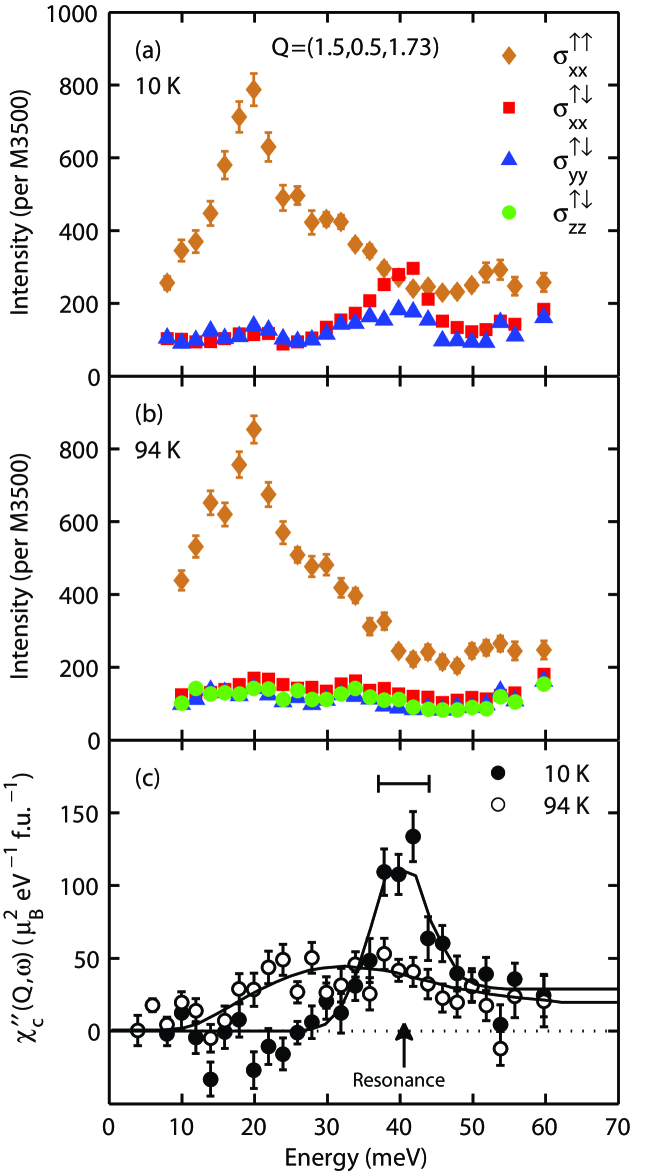
Figure 3: (Color online) Energy-dependent scans with polarization analysis collected at $\mathbf{Q}$=(1.5,0.5,1.73). (a-b) Spin-flip and non-spin-slip cross sections for various spin polarizations in the superconducting ($T=10$ K) and normal ($T=94$ K $=T_{c}+1$ K) states. (c) Out-of-plane generalized susceptibility $\chi_{c}$ determined from (a) and (b). The solid line for the $T=10$ K data is a resolution corrected fit to the cross-section described in the text. The horizontal bar represents the full-width-at-half maximum (FWHM) resolution for a $\delta(\omega-\omega_{0})$ cross section.

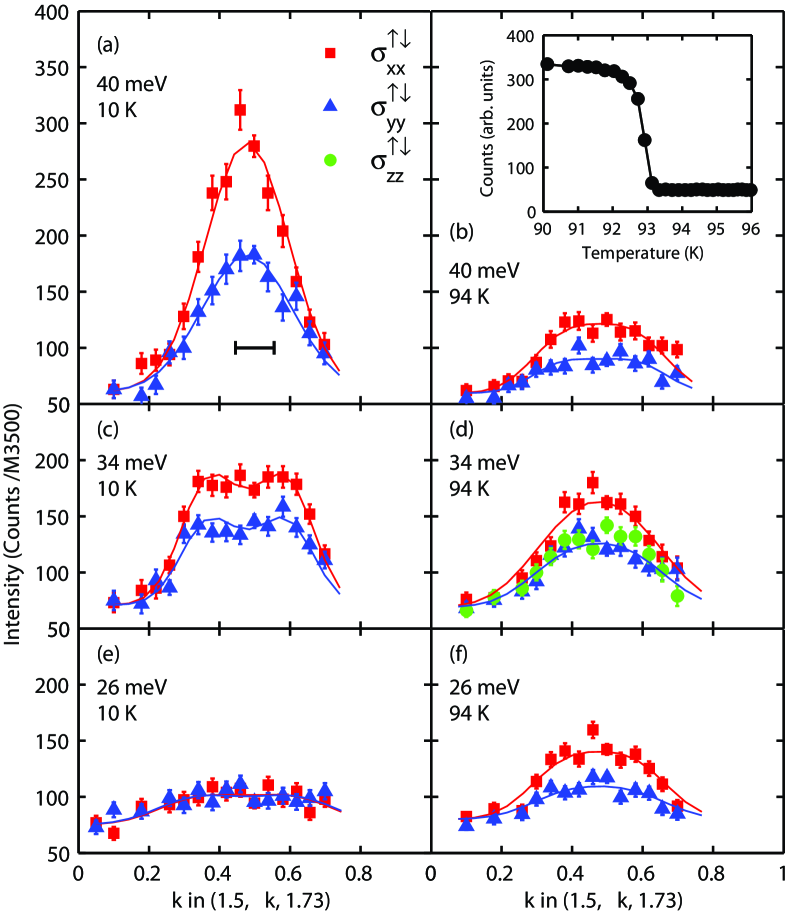
Figure 4: (Color online) (a)-(f) Wavevector-dependent scans with LPA through the (1.5,0.5,1.73) position at the resonance energy (a,b) and lower energies (c-f). The solid lines are resolution corrected fits to Eq. 10. The horizontal bar represents the FWHM resolution for a $\delta(\mathbf{Q}-\mathbf{Q}_{0})$ cross-section. The inset to (b) shows $T_{c}$ determined by a neutron depolarization technique in which the sample was field cooled through $T_{c}$ in a vertical field. The field was then rotated to be horizontal and the spin flip scattering on the (310) Bragg peak measured on warming.

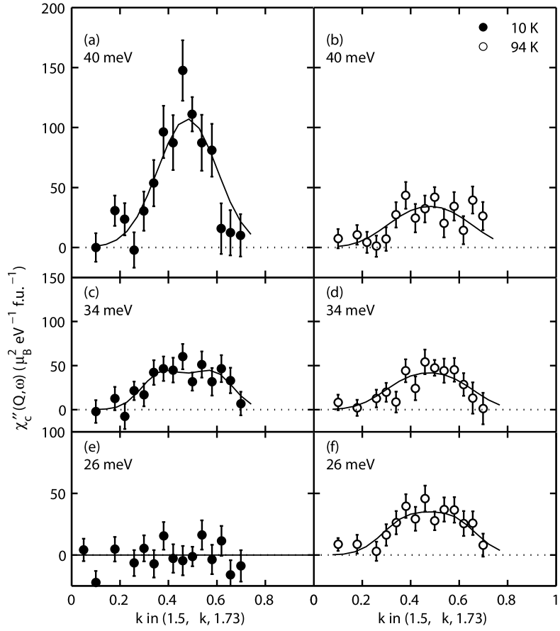
Figure 5: The out-of-plane response $\chi_{c}^{\prime\prime}$ in the normal and superconducting states determined from the data in Fig. 4. The solid lines are resolution corrected fits to the cross-section described in the text.

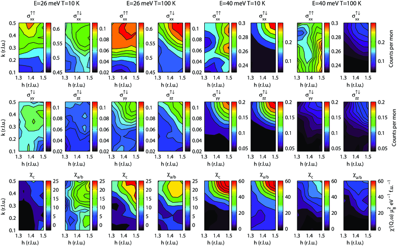
Figure 6: (Color online) (Top two rows) Spin polarized cross sections as defined in the text for $E$=26, 40 meV and $T$=10, 100 K. The $\uparrow\uparrow$ channel is mostly phonon scattering and the $\uparrow\downarrow$ channels are mostly magnetic scattering. (Bottom row) Magnetic responses $\chi_{a/b}^{\prime\prime}(\mathbf{q},\omega)$ and $\chi_{c}^{\prime\prime}(\mathbf{q},\omega)$ determined from top two rows. Note that some structure is due to statistical noise.

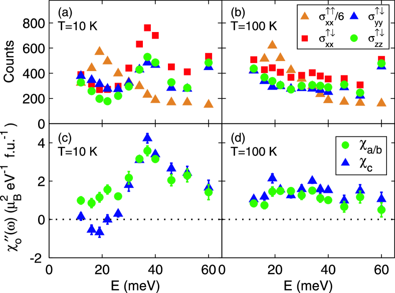
Figure 7: (Color online) (a)-(b) Integral of the spin-polarized cross sections over reciprocal space described in text and Fig. 2. (c)-(d) Local susceptibility determined from data in (a)-(b) via Eqs. II.1 and 11.

Fig. 3 shows energy-dependent scans made at the (1.5,0.5,1.73) position with various spin polarizations. At this position in reciprocal space the non spin-flip (phonon) scattering is up to 8 times stronger than the spin-flip scattering. Thus an unpolarized measurement made under the same conditions would be dominated by phonon scattering at some energies (the comparison with unpolarized experiments is discussed further in Appendix B). In the normal state the $\sigma_{xx}^{\uparrow\downarrow}$ cross section is larger than $\sigma_{yy}^{\uparrow\downarrow}$ and $\sigma_{zz}^{\uparrow\downarrow}$ over a wide energy range, $20\lesssim E\lesssim 60$ meV, signalling the presence of magnetic excitations. We can use Eq. 8 to isolate the out-of-plane response $\chi^{\prime\prime}_{c}$, this is shown in Fig. 3(c). In the superconducting state there is a large increase in $\sigma_{xx}^{\uparrow\downarrow}$ and $\sigma_{yy}^{\uparrow\downarrow}$ ($\sigma_{zz}^{\uparrow\downarrow}$ was not measured in this case) near the resonance energy. The difference scan Fig. 3(c) shows a sharp resonance peak at $E\approx 40$ meV which appears to have formed by a transfer of spectral weight from lower energies $E\lesssim 35$ meV. The $\chi_{c}^{\prime\prime}$ response appears to be largely gapped below about 30 meV. Similar data was obtained using unpolarized neutrons by Bourges et al. Bourges et al. (1999). We do not observe a collective magnetic excitation in the 50–60 meV range as observed recently in HgBa₂CuO_4+δ Li et al. (2010). We note that there is a peak in the non spin flip channel in this energy range in Fig. 3(a).

In order to analyze our data further, we fitted the $T=10$ K scan in Fig. 3(c) to the resolution-corrected model cross section

$$\begin{split}\chi_{c}(\mathbf{q},\omega)&=\left[A\delta(\omega-\omega_{0})+B\theta(\omega-\omega_{0})\right]\\ &\times\exp\left\{-\frac{(h-1/2)^{2}+(k-1/2)^{2}}{2\sigma^{2}}\right\},\end{split}$$ (9)

where $\theta$ is the heaviside step function and $\sigma$ is the width parameter extracted from a $\mathbf{q}$-dependent scan through the resonance (see Table 1). Throughout this paper we use the RESTRAX simulation package Saroun and Kulda (1997) to perform convolutions of the instrumental resolution function and model cross sections. Using the cross section defined by Eq. 9, we find that the width of the peak due to the resonance in Fig. 3(c) is resolution limited and $\hbar\omega_{0}=41\pm 1$ meV.

We have converted the data in Fig. 3(c) to absolute units using Eq. 1 without attempting to deconvolve the experimental resolution. This means that each point in the scan is an average (in wavevector and energy) over the instrumental resolution. Keeping this in mind, we have integrated the response in Fig. 3(c) in energy for $4<E<60$ meV for $T$=10 K and 94 K. From Eqs. 2 and 15, we find the out-of-plane fluctuating moments $\langle m^{2}_{c}\rangle$ are 0.50$\pm$0.05 and 0.48$\pm$0.05 $\mu_{B}^{2}$f.u.^-1 at $T$=10 K and 94 K respectively (these are averaged over the resolution width in wavevector shown in Fig. 4). Thus this increase in the response at the resonance energy can be accounted for by a shift in spectral weight from lower energies.

Fig. 4 shows wavevector dependent scans along the $(1.5,k,1.73)$ line at three characteristic energies. Fig. 5 shows the susceptibility extracted from the data in Fig. 4 using Eq. II.1. In the normal state ($T=94$ K), we observe a magnetic response at all three energies. On cooling to $T=10$ K, the lower frequency $E=26$ meV response is suppressed while the response at the resonance energy ($E=40$ meV) increases dramatically and the $\mathbf{q}$-width decreases. The data were fitted to a model consisting of four incommensurate peaks with locations $\mathbf{Q}_{\delta}=(1/2\pm\delta,1/2)$ and $(1/2,1/2\pm\delta)$ and width $\sigma$:

$$\chi^{\prime\prime}(\mathbf{q},\omega)=A\sum_{\mathbf{Q}_{\scriptstyle\delta}}\exp\left\{-\frac{(\mathbf{Q}-\mathbf{Q}_{\delta})^{2}}{2\sigma^{2}}\right\}.$$ (10)

The results of this fitting procedure are shown in Table 1

$T$(K)	$\hbar\omega$(meV)	$\delta$(r.l.u)	$\sigma$(r.l.u)
10	26	N/A	N/A
	34	$0.12\pm 0.02$	$0.059\pm 0.01$
	40	$0$	$0.114\pm 0.01$
94	26	$0.12$	$0.085\pm 0.01$
	34	$0.12$	$0.095\pm 0.01$
	40	$0.12$	$0.071\pm 0.01$
	40	$0$	$0.16\pm 0.02$

Table 1: Incommensurability $\delta$ and width $\sigma$ parameters obtained from fitting Eq. 10 to the scans in Fig. 4. Where no error is quoted, the parameter was fixed.

We first consider the scans at the resonance energy ($\hbar\omega$=40 meV). A single Gaussian peak ($\delta$=0) provides a good description of the scan in the superconducting state [Fig. 4(a) and Fig. 5(a)]. In the normal state, there is magnetic scattering at the resonance energy [Fig. 5(b)]. The existence of a magnetic response at this energy in optimally doped YBCO has been a subject of some debate Rossat-Mignod et al. (1991); Mook et al. (1993); Fong et al. (1995); Bourges et al. (1999); Dai et al. (2001) and we will discuss this later. It is clear from our data that the response at the resonance energy is broader in $\mathbf{q}$ and weaker in the normal state than the superconducting state. If we fit the 40 meV data using Eq. 10 with $\delta$=0, we find $\sigma$=0.18$\pm$0.02 and 0.115$\pm$0.01 for the normal and superconducting states respectively. Returning to the superconducting state data at lower energy, we find a single Gaussian peak ($\delta$=0) does not provide a good description of the $\hbar\omega$=34 meV ($T$=10 K) scans [Fig. 4(c) and Fig. 5(c)] in the superconducting state. Better fits are obtained when a finite incommensurability $\delta$=0.12$\pm$0.02 is used. This $\delta$ is in agreement with that obtained in other studies of optimally doped YBCO Dai et al. (2001); Woo et al. (2006). In the normal state [Fig. 4(b,d,f) and Fig. 5(b,d,f)] we see clear magnetic scattering at the three energies investigated. We do not see a two-peaked structure as in Fig. 4(c), instead the response appears to be broadened out into single peak which, in some cases [e.g. Fig. 4(b,f)], looks “flat topped”. To contrast the normal and superconducting state responses, we have fitted the scans with the value of $\delta$ determined from the $T$=10 K and $\hbar\omega$=34 meV scan. The normal state response is broader in all cases (see Table 1).

III.2 Local Susceptibility Measurements

In order to search for the diffuse contributions to the magnetic response, we sampled a grid of points near the (3/2,1/2) position where the response is generally stronger. Extended grids at two characteristic energies are shown in Fig. 6. For this part of the experiment we collected three spin-flip channels and we were able to extract $\chi_{a/b}^{\prime\prime}$ and $\chi_{c}^{\prime\prime}$. The lowest row of Fig. 6 shows the signal extracted via Eq. II.1. The data collected at $E=40$ meV shows that the response is strongest near the (1.5,0.5,1.73) position both in the normal and superconducting states. At $E=26$ meV, we see a normal state response which is spread out: see, for example, $\chi_{a/b}^{\prime\prime}(E=26\mbox{ meV},T=100~{}\mbox{K})$, where the upper part of the map shows signal. On entering the superconducting state $\chi_{c}^{\prime\prime}$ shows a much larger change than $\chi_{a/b}^{\prime\prime}$ suggesting that a spin anisotropy develops.

Fig. 7 shows the wavevector integrals collected at a number of energies over the grey region shown in Fig. 2. This is the region of highest intensity in the Brillouin zone, but there is clearly scattering in other parts of the zone. The contribution of the grey region to $\chi_{o}^{\prime\prime}(\omega)$ is shown in Fig. 7(c) and (d). Fig. 7 shows that there is a strong response in the normal state over a wide energy range. When compared to the energy-dependent scan at (1.5,0.5,1.73), we see that the higher energy response is relatively stronger. This is due to the presence of a broader response in $\mathbf{q}$ at higher energies $E\gtrsim 50$ meV Hayden et al. (2004); Reznik et al. (2004); Woo et al. (2006). On entering the superconducting state, we see a strong reduction in $\chi_{c}^{\prime\prime}$ with little change in $\chi_{a/b}^{\prime\prime}$. This means the magnetic response develops a strong spin anisotropy in the superconducting state (see Sec. IV.2 for more discussion). For higher energies, $E\geq 34$ meV, the response increases in the superconducting state, not only at the resonance energy, but up to 60 meV. Table 2 shows that when integrated over the range $12<E<60$ meV the total fluctuating moment $\langle m^{2}\rangle$ increases by about 60%. In order to compare with other studies of the resonance in near optimally doped YBCO Dai et al. (1999); Fong et al. (1999); Woo et al. (2006), we have also integrated the data in Fig. 7 over the smaller energy range $30<E<60$ meV (see Table 2) in this case we see a larger change in $\langle m^{2}\rangle$ (between the normal and superconducting states) which is comparable to previous reports Dai et al. (1999); Fong et al. (1999); Woo et al. (2006).

$T$(K)	$\langle m^{2}_{a/b}\rangle(\mu_{B}^{2}\;\mathrm{f.u.}^{-1})$	$\langle m^{2}_{c}\rangle(\mu_{B}^{2}\;\mathrm{f.u.}^{-1})$	$\langle m^{2}\rangle(\mu_{B}^{2}\;\mathrm{f.u.}^{-1})$
$12\leq\hbar\omega(\mathrm{meV})\leq 60$
10	$0.031\pm 0.004$	$0.026\pm 0.004$	$0.088\pm 0.007$
100	$0.017\pm 0.003$	$0.022\pm 0.003$	$0.056\pm 0.005$
$30\leq\hbar\omega(\mathrm{meV})\leq 60$
10	$0.024\pm 0.003$	$0.026\pm 0.003$	$0.074\pm 0.005$
100	$0.009\pm 0.002$	$0.014\pm 0.002$	$0.032\pm 0.003$

Table 2: Fluctuating moments $\langle m^{2}_{a/b}\rangle$, $\langle m^{2}_{c}\rangle$ and $\langle m^{2}\rangle=2\langle m^{2}_{a/b}\rangle+\langle m^{2}_{c}\rangle$ in the normal ($T=100$ K) and superconducting ($T=10$ K) states calculated by numerically integrating the response in Fig. 7. The errors quoted are statistical and do not include the systematic error in the absolute scale which is about $\pm 20$%.

IV Discussion

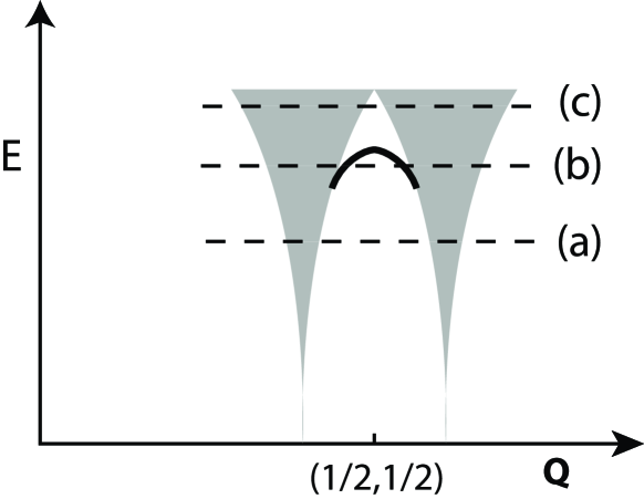
Figure 8: Schematic representation of $\chi^{\prime\prime}(\mathbf{q},\omega)$ in the superconducting state of YBa₂Cu₃O_6.9 based on Refs. Onufrieva and Pfeuty, 2002; Eremin et al., 2005. The black line is the resonance mode and grey area the particle-hole continuum. Scans (a), (b) and (c) correspond approximately to 20, 40 and 60 meV.

IV.1 Response in the Normal and Superconducting States

Theories of the magnetic excitations in the superconducting state of cuprate superconductors such as YBa₂Cu₃O_6+x are well developed Lavagna and Stemmann (1994); Demler and Zhang (1995); Liu et al. (1995); Mazin and Yakovenko (1995); Abanov and Chubukov (1999); Brinckmann and Lee (1999); Kao et al. (2000); Norman (2001); Tchernyshyov et al. (2001); Onufrieva and Pfeuty (2002); Eremin et al. (2005); Eschrig (2006). Many features are explained by a magnetic exciton scenario Liu et al. (1995); Mazin and Yakovenko (1995); Tchernyshyov et al. (2001); Onufrieva and Pfeuty (2002); Eremin et al. (2005) in which the resonance is a bound state in the particle-hole channel, which appears in a region of $\mathbf{q}-\omega$ space where there are no damping processes due to electron-hole pair creation. This is illustrated schematically in Fig. 8. In such a picture, significant magnetic response should also be present in the normal state. As the system enters the superconducting state we expect the low energy response to be suppressed below $E\lesssim\Delta$ and an enhancement of the response at the resonance energy. This is the behaviour seen in Figs. 3 and 5. The nature of the magnetic response in the normal state of optimally doped YBCO has been a subject of debate, particularly with regard to energies near the resonance energy Rossat-Mignod et al. (1991); Mook et al. (1993); Fong et al. (1995, 1996); Bourges et al. (1999); Dai et al. (2001). Some studies suggest there is a significant response Rossat-Mignod et al. (1991); Bourges et al. (1999) for $\mathbf{q}\approx(1/2,1/2)$ and $\hbar\omega\approx 40$ meV, while others claim the response is absent or too weak to observe Fong et al. (1995, 1996); Dai et al. (2001). The present experiment allows the magnetic response to be separated from phonon scattering. We find that the out-of-plane response $\chi^{\prime\prime}_{c}(\mathbf{q},\omega)$ is peaked around $\hbar\omega\approx 30$ meV for $\mathbf{q}\approx(1/2,1/2)$ in the normal state ($T=94$ K). On cooling there is a shift of spectral weight to higher energies which leads to the formation of the resonance peak near 40 meV, with the concomitant formation of incommensurate peaks observed at 34 meV and a spin gap below about 30 meV for the $\chi^{\prime\prime}_{c}$ component of the response. This is consistent with the formation of a magnetic excitonic mode as illustrated schematically in Fig. 8. The work presented in this paper refers to optimally doped YBCO where it is harder to separate the magnetic contribution from phonons and other background scattering than for other compositions. We note that for underdoped YBCO (e.g. YBa₂Cu₃O_6.6) Mook et al. (1998); Bourges et al. (2000); Hayden et al. (2004); Hinkov et al. (2007) a strong dispersive excitonic mode is also observed in the superconducting state. On warming to $T_{c}$ the remnants of this mode are clearly observable and persist well above $T_{c}$.

The discussion above relates to the energy- and wavevector- dependent scans presented in Sec. III.1. These yield information about the out-of-plane fluctuations described by $\chi^{\prime\prime}_{c}$. We did not collect the corresponding scans for $\chi^{\prime\prime}_{a/b}$, however, we did probe this component of the local susceptibility in the measurements presented in Sec. III.2. These measurements were designed to yield estimates for the total response in a region of $\mathbf{q}$ space rather than identify the location of specific features such as incommensurate peaks. They are summarized in Fig. 7(c) and (d). In Fig. 7(c) we see that there is strong evidence for additional scattering below 30 meV in the $\chi^{\prime\prime}_{a/b}$ component of the response. This response appears to be rather spread out in wavevector when we inspect the corresponding map ($\hbar\omega=$26 meV, $T=10$ K) in Fig. 6. Thus our results suggest that there are other (diffuse) contributions to the $\chi^{\prime\prime}_{a/b}$ response at low energies in the superconducting state. The $\chi^{\prime\prime}_{a/b}$ component of the response has a lower ‘spin gap’ than the $\chi^{\prime\prime}_{c}$ component. The low energy response ($E\lesssim 30$ meV) may be due to the electron-hole continuum also present in theories of the resonance Tchernyshyov et al. (2001); Onufrieva and Pfeuty (2002); Eremin et al. (2005). This is illustrated schematically in Fig. 8.

IV.2 Spin Anisotropy in YBa₂Cu₃O_6.9

Our results suggest that a spin anisotropy develops in the lower energy ($10$$\lesssim$$E$$\lesssim$30 meV) excitations on entering the superconducting state. Nuclear magnetic resonance (NMR) probes the spin fluctuations in the very low frequency limit and, indeed, the anisotropy of spin-lattice relaxation rate ($T_{1}$) in YBa₂Cu₃O₇ has been reported to show a strong temperature dependence in the superconducting state Barrett et al. (1991); Takigawa et al. (1991). Various theories have attributed this to the combined effect of the NMR form factor and a changing $\chi^{\prime\prime}(\mathbf{q},\omega)$ (See e.g. Ref. Bulut and Scalapino, 1992; Thelen et al., 1993). However, the present measurements show that there is also an significant intrinsic anisotropy in $\chi_{\alpha}^{\prime\prime}(\mathbf{q},\omega)$ with respect to the spin direction which must be considered. It is interesting to note that Uldry et al. Uldry et al. (2005) have extracted the intrinsic anisotropy from NMR data and concluded that the out-of-plane correlations do not change appreciably on entering the superconducting state, in contrast to our results. This may be because NMR measurements probe the excitations at much lower frequencies than our measurements.

Anisotropy in the susceptibility ultimately comes from the spin-orbit interaction. An exotic case is the superfluid ³He A-phase Vollhardt and Woelfle (1990), where the susceptibility depends on the orientation of the angle of the field to the characteristic spin vector $\mathbf{d}$. In the case of superconductors, dramatic changes in a pre-existing spin anisotropy have recently been observed in BaFe_1.9Ni_0.1As₂ Lipscombe et al. (2010) and a small anisotropy at the resonance energy is observed in FeSe_0.5Te_0.5 Babkevich et al. . A possible origin of the emergence of spin anisotropy in YBa₂Cu₃O_6.9 may be the Dzyaloshinskii-Moriya (DM) interactions between the copper spins Coffey et al. (1991). The buckled structure of the CuO₂ planes in ortho-I YBa₂Cu₃O_6.9 (see Fig. 1) means that DM interactions of the form $\mathbf{D}\cdot\mathbf{S}_{i}\times\mathbf{S}_{j}$ are allowed between neighbouring Cu spins. The presence of such terms leads to additional spin anisotropy. This leads to a polarization dependence to the spin wave dispersion and energy in the antiferromagnetic parent compounds La₂CuO₄ Peters et al. (1988) and YBa₂Cu₃O_6.2 Shamoto et al. (1993). In the case of YBa₂Cu₃O_6.2 the anisotropy gaps are $\sim$10 meV Shamoto et al. (1993) and the ordered moments lies along the [100] direction Janossy et al. (1999).

The low energy excitations ($E\lesssim$30 meV) we observe have their predominant fluctuations within the CuO₂ planes making the $a/b$ response largest. At higher energies, $E\approx$40 meV, the excitations are more isotopic. This corresponds to all three components of the spin-triplet $\{|\uparrow\uparrow\rangle,|\uparrow\downarrow\rangle-\downarrow\uparrow\rangle,|\downarrow\downarrow\rangle\}$ being excited.

V Conclusion

In this work we used inelastic neutron scattering with longitudinal polarization analysis to measure the magnetic excitations in the normal and superconducting states of near optimally doped YBa₂Cu₃O_6.9. We have unambiguously identified a strong magnetic response in the normal state which appears to exist over the 10–60 meV range of the present experiment. On entering the superconducting state, the out-of-plane magnetic response ($\chi_{c}^{\prime\prime}$), is strongly suppressed at lower energies, while the response at the magnetic resonance energy and above increases. We also find evidence for a new diffuse component to the magnetic response in the $\chi_{a/b}^{\prime\prime}$ component of the susceptibility at low energies 10$\lesssim$$E$$\lesssim$30 meV which is present in the superconducting state.

VI Acknowledgements

We would like to acknowledge helpful discussion with James Annett, Anthony Carrington, PengCheng Dai, Chris Lester, Jan Šaroun, Nic Shannon and Qimiao Si.

Appendix A Sum Rules and the Magnetic Response

A.1 Local Susceptibility

The local susceptibility is a useful way to characterise the overall response. It is defined as,

$$\chi^{\prime\prime}(\omega)=\frac{\int\chi^{\prime\prime}(\mathbf{Q},\omega)\;d^{3}\mathbf{Q}}{\int d^{3}\mathbf{Q}},$$ (11)

where, in general, the integrals are over a volume of reciprocal space which samples the full $\mathbf{Q}$ dependence of $\chi^{\prime\prime}(\mathbf{Q},\omega)$. In the case of YBa₂Cu₃O_6+x this is one unit cell in the $ab$ plane and infinity along $c$. The local susceptibility can be split into the two terms of Eq. 5. Thus integrating Eq. 5 we have

$$\chi^{\prime\prime}(\omega)=\chi_{o}^{\prime\prime}(\omega)+\chi_{e}^{\prime\prime}(\omega),$$ (12)

where

$$\chi_{o}^{\prime\prime}(\omega)=\frac{1}{2}\int_{0}^{1}\;dh\int_{0}^{1}dk\;\chi_{o}^{\prime\prime}(h,k,\omega).$$ (13)

The definition for $\chi_{o}^{\prime\prime}(\omega)$ used here differs by a factor 2 from earlier work, but allows a direct comparison with single layer compounds Vignolle et al. (2007).

A.2 Total Moment Sum Rule

For an ion with spin only moment, the total squared moment is

$$\langle m^{2}\rangle = g^{2}\mu^{2}_{B}S(S+1)$$ (14)

$$= 3\mu_{B}^{2}\mbox{ for }S=\frac{1}{2}\mbox{ and }g=2.$$

The total fluctuating moment observed by INS over a given range of energy and momentum can be determined from the fluctuation-dissipation theorem and is

$$\langle m^{2}\rangle = \langle m_{x}^{2}+m_{y}^{2}+m_{z}^{2}\rangle$$ (15)

$$= \frac{1}{\pi}\int\left[\frac{\chi_{xx}^{\prime\prime}(\omega)+\chi_{yy}^{\prime\prime}(\omega)+\chi_{zz}^{\prime\prime}(\omega)}{1-\exp(-\hbar\omega/kT)}\right]\;d\omega.$$

Appendix B Comparison with Unpolarized Studies

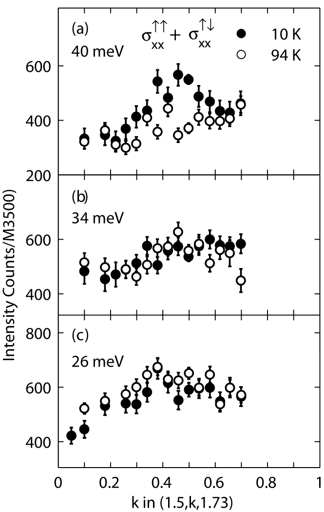
Figure 9: Wavevector-dependent scans of $\sigma_{xx}^{\uparrow\uparrow}+\sigma_{xx}^{\uparrow\downarrow}$ at various energies. This combination allows comparison with unpolarized studies.

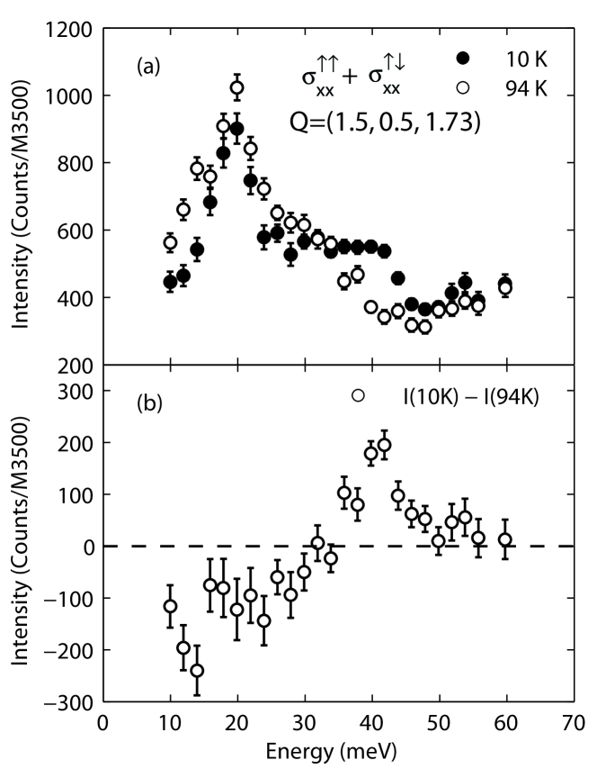
Figure 10: (a) Energy-dependent scans of $\sigma_{xx}^{\uparrow\uparrow}+\sigma_{xx}^{\uparrow\downarrow}$ at $\mathbf{Q}$=(1.5,0.5,1.73) at $T=10,94$ K. (b) Difference of scans in (a).

There are many unpolarized studies of the magnetic excitations in YBa₂Cu₃O_6+x Rossat-Mignod et al. (1991); Fong et al. (1995); Stock et al. (2005); Dai et al. (2001); Reznik et al. (2004). In this section we show that our results are broadly consistent with previous results. The main issues that arise in unpolarized studies are: (i) the separation of magnetic signal from background and (ii) the separation of magnetic and phonon scattering. In the present spin-polarized study we may compare to different spin-flip cross-sections to remove the background and the phonon contribution. This is demonstrated in Eqs. 3-II.1.

The unpolarized inelastic cross section is generally of the form

$$\left(\frac{d^{2}\sigma}{d\Omega dE}\right)\propto\frac{\chi^{\prime\prime}(\mathbf{q},\omega,T)}{1-\exp(-\hbar\omega/kT)}+N(q,\omega,T),$$ (16)

where the first term represents the inelastic magnetic response and the second that due to the phonons. A sharp magnetic response such as the resonance can be isolated through $\mathbf{q}$ and $\omega$ scans and verified as being magnetic through the form factor present in Eq. 1. However, a broad or diffuse response is more difficult to distinguish from phonons. The phonon response $N(q,\omega,T)$ usually decreases with temperature ($\hbar\omega\lesssim kT$) or remains constant ($\hbar\omega\gg kT$) due to the Bose factor. Thus a signal that increases with decreasing temperature (such as the resonance) is likely to be magnetic. If a magnetic signal decreases with decreasing temperature] such as the response below about 30 meV in Fig. 3(c)] it is difficult to distinguish from phonons using unpolarized neutrons.

In Figs. 9 and 10, we have reconstructed ‘unpolarized’ scans by adding together the spin-flip and non-spin-flip intensities for $\mathbf{H}\parallel x$, $\sigma_{xx}^{\uparrow\uparrow}+\sigma_{xx}^{\uparrow\downarrow}$. Our experiment was not optimized for this reconstruction because the spin-flip channels were counted longer than non-spin-flip, nevertheless we can make some useful observations. As expected, Fig. 9(a) clearly shows the resonance at $T=10$ K and $E=40$ meV in the superconducting state. Note there is increased background or phonon scattering at larger $k$ in this scan. In the normal state, at $T=94$ K, it is not possible to identify any magnetic scattering. For $E=34$ meV [Fig. 9(b)], the scans at both temperatures are similar. The data are consistent with a broad magnetic response which changes little between the two temperatures [see Fig. 5(c)-(d)]. Finally, for $E=26$ meV we observe a decrease in intensity across much of the scan on lowering the temperature. This is consistent with a reduction of the magnetic response at this energy [see Fig. 5(e)-(f)]. However, the phonon scattering at this energy and wavevector is strong [see Fig. 3(a)] thus part (about 50%) the reduction observed using unpolarized spectroscopy is due to the change of the Bose factor for the phonons.

Fig. 10 shows energy-dependent scans at the $\mathbf{Q}$=(1.5,0.5,1.73) position and a temperature difference often used to isolate the resonance (see e.g. Fong et al. (1995, 1999)). From Figs. 3 and 4, we can deduce that about 50% of the observed change observed with temperature at 26 meV is due to phonons.

References

- (1) See e.g. Handbook of high-temperature superconductivity: theory and experiment, edited by John Robert Schrieffer, James S. Brooks (Springer, New York, 2007). Superconductivity, edited by K. H. Bennemann and J.B. Ketterson (Springer, Berlin, 2008), Vols. 1 & 2.
- Headings et al. (2010) N. S. Headings, S. M. Hayden, R. Coldea, and T. G. Perring, Phys. Rev. Lett. 105, 247001 (2010).
- Cheong et al. (1991) S. W. Cheong, G. Aeppli, T. E. Mason, H. Mook, S. M. Hayden, P. C. Canfield, Z. Fisk, K. N. Clausen, and J. L. Martinez, Phys. Rev. Lett. 67, 1791 (1991).
- Rossat-Mignod et al. (1991) J. Rossat-Mignod, L. P. Regnault, C. Vettier, P. Bourges, P. Burlet, J. Bossy, J. Y. Henry, and G. Lapertot, Physica C: Superconductivity 185-189, 86 (1991).
- Mook et al. (1993) H. A. Mook, M. Yethiraj, G. Aeppli, T. E. Mason, and T. Armstrong, Phys. Rev. Lett. 70, 3490 (1993).
- Fong et al. (1995) H. F. Fong, B. Keimer, P. W. Anderson, D. Reznik, F. Dogbrevean, and I. A. Aksay, Phys. Rev. Lett. 75, 316 (1995).
- Bourges et al. (1997) P. Bourges, H. F. Fong, L. P. Regnault, J. Bossy, C. Vettier, D. L. Milius, I. A. Aksay, and B. Keimer, Phys. Rev. B 56, R11439 (1997).
- Mook et al. (1998) H. A. Mook, P. C. Dai, S. M. Hayden, G. Aeppli, T. G. Perring, and F. Dogan, Nature 395, 580 (1998).
- Dai et al. (1999) P. C. Dai, H. A. Mook, S. M. Hayden, G. Aeppli, T. G. Perring, R. D. Hunt, and F. Dogan, Science 284, 1344 (1999).
- Hayden et al. (2004) S. M. Hayden, H. A. Mook, P. C. Dai, T. G. Perring, and F. Dogan, Nature 429, 531 (2004).
- Vignolle et al. (2007) B. Vignolle, S. M. Hayden, D. F. McMorrow, H. M. Ronnow, B. Lake, C. D. Frost, and T. G. Perring, Nat. Phys. 3, 163 (2007).
- Fauqué et al. (2007) B. Fauqué, Y. Sidis, L. Capogna, A. Ivanov, K. Hradil, C. Ulrich, A. I. Rykov, B. Keimer, and P. Bourges, Phys. Rev. B 76, 214512 (2007).
- Xu et al. (2009) G. Xu, G. D. Gu, M. Hucker, B. Fauque, T. G. Perring, L. P. Regnault, and J. M. Tranquada, Nat. Phys. 5, 642 (2009).
- Stock et al. (2005) C. Stock, W. J. L. Buyers, R. A. Cowley, P. S. Clegg, R. Coldea, C. D. Frost, R. Liang, D. Peets, D. Bonn, W. N. Hardy, and R. J. Birgeneau, Phys. Rev. B 71, 024522 (2005).
- Woo et al. (2006) H. Woo, P. Dai, S. M. Hayden, H. A. Mook, T. Dahm, D. J. Scalapino, T. G. Perring, and F. Dogan, Nat. Phys. 2, 600 (2006).
- Hayden et al. (1996) S. M. Hayden, G. Aeppli, H. A. Mook, T. G. Perring, T. E. Mason, S. W. Cheong, and Z. Fisk, Phys. Rev. Lett. 76, 1344 (1996).
- Fong et al. (1999) H. F. Fong, P. Bourges, Y. Sidis, L. P. Regnault, A. Ivanov, G. D. Gu, N. Koshizuka, and B. Keimer, Nature 398, 588 (1999).
- He et al. (2002) H. He, P. Bourges, Y. Sidis, C. Ulrich, L. P. Regnault, S. Pailhes, N. S. Berzigiarova, N. N. Kolesnikov, and B. Keimer, Science 295, 1045 (2002).
- Yu et al. (2010) G. Yu, Y. Li, E. M. Motoyama, X. Zhao, N. Bariscaronicacute, Y. Cho, P. Bourges, K. Hradil, R. A. Mole, and M. Greven, Phys. Rev. B 81, 064518 (2010).
- Blume (1963) M. Blume, Physical Review 130, 1670 (1963).
- Maleyev et al. (1963) S. V. Maleyev, V. G. Baryakhtar, and A. Suris, Sov. Phys. Solid State 4, 2533 (1963).
- Moon et al. (1969) R. M. Moon, T. Riste, and W. C. Koehler, Physical Review 181, 920 (1969).
- Squires (1978) G. L. Squires, Introduction to the theory of thermal neutron scattering (Cambridge, 1978).
- Lorenzo et al. (2007) J. E. Lorenzo, C. Boullier, L. P. Regnault, U. Ammerahl, and A. Revcolevschi, Phys. Rev. B 75, 054418 (2007).
- (25) We have also neglected nuclear-magnetic interference terms and chiral correlations. See e.g. Ref. Lorenzo et al. (2007).
- Bulut and Scalapino (1996) N. Bulut and D. J. Scalapino, Phys. Rev. B 53, 5149 (1996).
- Millis and Monien (1996) A. J. Millis and H. Monien, Phys. Rev. B 54, 16172 (1996).
- Brinckmann and Lee (2001) J. Brinckmann and P. A. Lee, Phys. Rev. B 65, 014502 (2001).
- Eremin et al. (2007) I. Eremin, D. K. Morr, A. V. Chubukov, and K. Bennemann, Phys. Rev. B 75, 184534 (2007).
- Pailhès et al. (2004) S. Pailhès, Y. Sidis, P. Bourges, V. Hinkov, A. Ivanov, C. Ulrich, L. P. Regnault, and B. Keimer, Phys. Rev. Lett. 93, 167001 (2004).
- Pailhès et al. (2006) S. Pailhès, C. Ulrich, B. Fauque, V. Hinkov, Y. Sidis, A. Ivanov, C. T. Lin, B. Keimer, and P. Bourges, Phys. Rev. Lett. 96, 257001 (2006).
- Babu et al. (2000) N. H. Babu, M. Kambara, P. J. Smith, D. A. Cardwell, and Y. Shi, J. Mater. Res. 15, 1235 (2000).
- Jorgensen et al. (1990) J. D. Jorgensen, B. W. Veal, A. P. Paulikas, L. J. Nowicki, G. W. Crabtree, H. Claus, and W. K. Kwok, Phys. Rev. B 41, 1863 (1990).
- Meuffels et al. (1989) P. Meuffels, R. Naeven, and H. Wenzl, Physica C 161, 539 (1989).
- Liang et al. (2006) R. Liang, D. A. Bonn, and W. N. Hardy, Phys. Rev. B 73, 180505 (2006).
- Lipscombe et al. (2010) O. J. Lipscombe, L. W. Harriger, P. G. Freeman, M. Enderle, C. Zhang, M. Wang, T. Egami, J. Hu, T. Xiang, M. R. Norman, and P. Dai, Phys. Rev. B 82, 064515 (2010).
- Bourges et al. (1999) P. Bourges, Y. Sidis, H. F. Fong, B. Keimer, L. P. Regnault, J. Bossy, A. S. Ivanov, D. L. Milius, and I. A. Aksay, AIP Conference Proceedings 483, 207 (1999).
- Li et al. (2010) Y. Li, V. Baledent, G. Yu, N. Barisic, K. Hradil, R. A. Mole, Y. Sidis, P. Steffens, X. Zhao, P. Bourges, and M. Greven, Nature 468, 283 (2010).
- Saroun and Kulda (1997) J. Saroun and J. Kulda, Physica B 234-236, 1102 (1997).
- Dai et al. (2001) P. Dai, H. A. Mook, R. D. Hunt, and F. Dogan, Phys. Rev. B 63, 054525 (2001).
- Reznik et al. (2004) D. Reznik, P. Bourges, L. Pintschovius, Y. Endoh, Y. Sidis, T. Masui, and S. Tajima, Phys. Rev. Lett. 93, 207003 (2004).
- Onufrieva and Pfeuty (2002) F. Onufrieva and P. Pfeuty, Phys. Rev. B 65, 054515 (2002).
- Eremin et al. (2005) I. Eremin, D. K. Morr, A. V. Chubukov, K. H. Bennemann, and M. R. Norman, Phys. Rev. Lett. 94, 147001 (2005).
- Lavagna and Stemmann (1994) M. Lavagna and G. Stemmann, Phys. Rev. B 49, 4235 (1994).
- Demler and Zhang (1995) E. Demler and S.-C. Zhang, Phys. Rev. Lett. 75, 4126 (1995).
- Liu et al. (1995) D. Z. Liu, Y. Zha, and K. Levin, Phys. Rev. Lett. 75, 4130 (1995).
- Mazin and Yakovenko (1995) I. I. Mazin and V. M. Yakovenko, Phys. Rev. Lett. 75, 4134 (1995).
- Abanov and Chubukov (1999) A. Abanov and A. V. Chubukov, Phys. Rev. Lett. 83, 1652 (1999).
- Brinckmann and Lee (1999) J. Brinckmann and P. A. Lee, Phys. Rev. Lett. 82, 2915 (1999).
- Kao et al. (2000) Y.-J. Kao, Q. Si, and K. Levin, Phys. Rev. B 61, R11898 (2000).
- Norman (2001) M. R. Norman, Phys. Rev. B 63, 092509 (2001).
- Tchernyshyov et al. (2001) O. Tchernyshyov, M. R. Norman, and A. V. Chubukov, Phys. Rev. B 63, 144507 (2001).
- Eschrig (2006) M. Eschrig, Advances in Physics 55, 47 (2006).
- Fong et al. (1996) H. F. Fong, B. Keimer, D. Reznik, D. L. Milius, and I. A. Aksay, Phys. Rev. B 54, 6708 (1996).
- Bourges et al. (2000) P. Bourges, Y. Sidis, H. F. Fong, L. P. Regnault, J. Bossy, A. Ivanov, and B. Keimer, Science 288, 1234 (2000).
- Hinkov et al. (2007) V. Hinkov, P. Bourges, S. Pailhes, Y. Sidis, A. Ivanov, C. D. Frost, T. G. Perring, C. T. Lin, D. P. Chen, and B. Keimer, Nat. Phys. 3, 780 (2007).
- Barrett et al. (1991) S. E. Barrett, J. A. Martindale, D. J. Durand, C. H. Pennington, C. P. Slichter, T. A. Friedmann, J. P. Rice, and D. M. Ginsberg, Phys. Rev. Lett. 66, 108 (1991).
- Takigawa et al. (1991) M. Takigawa, J. L. Smith, and W. L. Hults, Phys. Rev. B 44, 7764 (1991).
- Bulut and Scalapino (1992) N. Bulut and D. J. Scalapino, Phys. Rev. Lett. 68, 706 (1992).
- Thelen et al. (1993) D. Thelen, D. Pines, and J. P. Lu, Phys. Rev. B 47, 9151 (1993).
- Uldry et al. (2005) A. Uldry, M. Mali, J. Roos, and P. F. Meier, J. Phys: Cond. Mat. 17, L499 (2005).
- Vollhardt and Woelfle (1990) D. Vollhardt and P. Woelfle, The Superfluid Phases Of Helium 3 (Taylor and Francis, 1990).
- (63) P. Babkevich, B. Roessli, S. N. Gvasaliya, L.-P. Regnault, P. G. Freeman, E. Pomjakushina, K. Conder, and A. T. Boothroyd, arXiv:1010.6204v1 .
- Coffey et al. (1991) D. Coffey, T. M. Rice, and F. C. Zhang, Phys. Rev. B 44, 10112 (1991).
- Peters et al. (1988) C. J. Peters, R. J. Birgeneau, M. A. Kastner, H. Yoshizawa, Y. Endoh, J. Tranquada, G. Shirane, Y. Hidaka, M. Oda, M. Suzuki, and T. Murakami, Phys. Rev. B 37, 9761 (1988).
- Shamoto et al. (1993) S. Shamoto, M. Sato, J. M. Tranquada, B. J. Sternlieb, and G. Shirane, Phys. Rev. B 48, 13817 (1993).
- Janossy et al. (1999) A. Janossy, F. Simon, T. Feher, A. Rockenbauer, L. Korecz, C. Chen, A. J. S. Chowdhury, and J. W. Hodby, Phys. Rev. B 59, 1176 (1999).