Path lengths, correlations, and centrality in temporal networks

Abstract

In temporal networks, where nodes interact via sequences of temporary events, information or resources can only flow through paths that follow the time-ordering of events. Such temporal paths play a crucial role in dynamic processes. However, since networks have so far been usually considered static or quasi-static, the properties of temporal paths are not yet well understood. Building on a definition and algorithmic implementation of the average temporal distance between nodes, we study temporal paths in empirical networks of human communication and air transport. Although temporal distances correlate with static graph distances, there is a large spread, and nodes that appear close from the static network view may be connected via slow paths or not at all. Differences between static and temporal properties are further highlighted in studies of the temporal closeness centrality. In addition, correlations and heterogeneities in the underlying event sequences affect temporal path lengths, increasing temporal distances in communication networks and decreasing them in the air transport network.

I Introduction

Understanding complex networks is of fundamental importance for studying the behavior of various biological, social and technological systems Newman06a ; Dorogovtsev03 ; Newman10 . Often, networks represent the complex lattices on which some dynamical processes unfold BBV08 , from information flow to epidemic spreading. For such processes, networks have mainly been considered static or quasi-static, such that dynamic changes of the network structure take place at a time scale longer than that of the studied process, and thus a node may interact with any or all of its neighbors at any point in time. In empirical analysis of systems where time-stamped data is available, a common approach has been to integrate connections or interaction events over the period of observation. This results in a static network where a pair of nodes is connected by a link if an event has been observed between them at any point in time. The frequency of events between nodes may then be taken into account with link weights that represent the number of events between nodes (see, e.g., Barrat04 ; Onnela07 ) Taking a step beyond static networks, in the dynamic network view (see, e.g. Gautreau09 ; Rosvall10 ), links are allowed to form and terminate in time, such as friendships forming and decaying in social networks. This view is commonly adopted in epidemiological modeling in the form of concurrency or transmission graphs Morris95 ; Riolo01 – e.g. for sexually transmitted diseases, links represent partnerships that have a beginning and an end, and the prevalence of multiple simultaneous partnerships has significant effects on the dynamics of outbreaks.

However, there are many cases where even the dynamic network picture is too coarse-grained, as the nodes are in reality connected by recurrent, temporary events of short duration at specific times only Kempe00 ; Kempe02 ; Holme05a ; Vazquez07 ; Iribarren09 ; Karsai10 ; HolmePNAS10 ; HolmeSimulated10 . We use the term temporal network for such systems to distinguish them from static or (quasi-static) dynamic networks. The events in a temporal network represent the temporal sequence of interactions between nodes, and thus the dynamics of any process mediated by such interactions depends on their structure. As an example, in an air transport network, events may represent individual flights transporting passengers In a social network, events may represent individual social interactions (phone calls, emails, physical proximity) that allow information to propagate through the network from one individual to another. In epidemiological modeling, data on the timings of possible transmission events, i.e. individual encounters that may result in disease transmission, has allowed for moving beyond the concurrency graph view HolmePNAS10 ; HolmeSimulated10 .

An immediate consequence of event-mediated interactions for any dynamics is that it has to follow time-ordered, causal paths Kempe02 ; Holme05a . Because of the causality requirement, the static network representation where nodes are connected if any interaction has been observed between them at any point in time can be misleading: although node $i$ may be connected to node $j$ via some path in the static network, that path may not exist in its temporal counterpart. Nevertheless, were the interaction events uncorrelated and uniformly spread in time, they could in many cases be taken into account by assigning weights to the edges of the static network, so that the weights would represent the frequencies of events between nodes Barrat04 ; Onnela07 and regulate the rate of interactions. However, it has turned out that this is commonly not the case: it has been observed that for the dynamics of spreading of computer viruses, information, or diseases, timings of the actual events and their temporal heterogeneities Moody02 ; HolmePNAS10 ; HolmeSimulated10 ; Vazquez07 ; Iribarren09 ; Karsai10 ; Miritello10 play an important role – e.g., the burstiness of human communication has been observed to slow down the maximal rate of information spreading Iribarren09 ; Karsai10 ; Miritello10 . Hence, for a detailed understanding of such processes, one should adopt the temporal network view.

A temporal network can be represented by a set of $N$ nodes between which a complete trace of all interaction events $\mathcal{E}$ occurring within the time interval $[0,T]$ is known. Each such event can be represented by a quadruplet $e\equiv(u,v,t,\delta t)$, where the event connecting nodes $u$ and $v$ begins at $t$ and the interaction is completed in time $\delta t$. As an example, $\delta t$ may correspond to the duration of a flight in an air transport network or the time between an user sending an email and the recipient reading it. Broadly, we define $\delta t$ such that if an event $e$ transmits something from $u$ to $v$, the recipient receives the transmission only after a time $\delta t$. However, in some cases, events can be approximated as instantaneous so that $\delta t=0$ and they can be represented with triplets $e\equiv(u,v,t)$, as in Ref. Holme05a . Further, events can be directed or undirected depending on whether the transmission or flow is directed or not.

In some earlier papers Tang10a ; Tang10 ; Kostakos09 , temporal networks have been represented as a set of graphs $\mathcal{G}=\langle G_{0},\dots,G_{T}\rangle$, where $G_{t}=(V_{t},E_{t})$ is the graph of pairwise interactions between the nodes at time $t\in[0,T]$. Here, $V_{t}$ and $E_{t}$ represent the nodes and edges at time $t$, respectively. However, this picture is only meaningful when the events are instantaneous (and, for practical purposes, only when the time is discretized). If the events have a duration $\delta t$ such a representation cannot be applied: it is not compatible with the fact that for anything to be transmitted via node $i$ to node $j$, $i$ has to receive the transmission before the event connecting $i$ and $j$ is initiated, but $j$ then receives the transmission only after a time $\delta t$.

In this paper, we set out to study the time-ordered paths that span a temporal graph and their durations. Any dynamical processes have to proceed along such paths; consider, as an example, the deterministic susceptible-infectious (SI) dynamics, where infected nodes always infect their susceptible neighbors as soon as they interact. The speed of such dynamics depends on how long it on average takes to complete time-ordered shortest paths between nodes, i.e. the average temporal distance between nodes, which in turn depends on the temporal heterogeneity and correlations of the event sequence. As an example, in a social network, where events such as calls or emails mediate information, the average temporal distance measures the shortest time it takes for any information to be passed from one individual to another, either directly or via intermediaries. For other dynamics, additional constraints can be placed on allowed transmission paths: e.g., for the susceptible-infectious-recovered (SIR) spreading dynamics where an infected node remains infectious for a limited period of time only, there is a waiting time threshold between consecutive events spanning a path.

We begin by defining the average temporal distance between nodes that properly takes the finiteness of the period of observation into account. We also present an algorithm for calculating such distances in event sequences, based on the concept of vector clocks. We then compare static and temporal distances in empirical networks of human communication and air transport and illustrate the differences. We next turn to the role of heterogeneities and correlations in the event sequences, and show that their effects are strikingly different in our empirical networks: contrary to the known effect of correlations slowing down dynamics in human communications, they give rise to faster dynamics in the air transport network. The roles of correlations are also studied on temporal paths constrained by a SIR-like condition on allowed waiting times between events. Finally, we study the temporal centrality of nodes, and show that nodes that may appear insignificant from the static point of view may in fact provide fast temporal paths to all other nodes.

II Measuring distances in temporal graphs

II.1 Temporal paths and temporal distances: definitions

Information or resources can be transmitted from node $i$ to node $j$ in a temporal network only if they are joined by a causal temporal path, i.e. a time-ordered sequence of events beginning at $i$ and ending at $j$ Kempe02 ; Holme05a . If the events are non-instantaneous, a temporal path exists only if there is a time-ordered sequence where each event begins only after the previous one is completed. As an example, suppose that there is an event $e_{1}=(i,j,t_{1},\delta t_{1})$ between nodes $i$ and $j$ and another event $e_{2}=(j,k,t_{2},\delta t_{2})$, between $j$ and $k$. This sequence of events spans the temporal path $i\rightarrow j\rightarrow k$ only if $t_{2}>t_{1}+\delta t_{1}$, and the time it takes to complete this path, i.e. the temporal path length, is then $\Delta t=t_{2}-t_{1}+\delta t_{2}$. Let us define the temporal distance $\tau_{ij}(t)$ between $i$ and $j$ as the shortest time it takes to reach $j$ from $i$ at time $t$ along temporal paths. If the fastest sequence of events, i.e. the shortest temporal path joining $i$ and $j$ begins at time $t^{\prime}>t$ and its duration is $\delta t$, then $\tau_{ij}=\left(t^{\prime}-t\right)+\delta t$. It is evident that this temporal distance depends on the time of measurement $t$; it may also happen that no such path exists and then $\tau_{ij}(t)=\infty$. As $\tau_{ij}(t)$ is not constant in time, it is useful to characterize temporal distances with an average temporal distance $\tau_{ij}$, averaged over the entire period of observation. However, taking this average is not straightforward and certain choices have to be made.

For empirical event sequences, the period of observation $[0,T]$ is always finite. Because of this, the total number of future events decreases as time increases, and consequently so does the likelihood of the existence of a time-ordered path between any pair of nodes. Thus, infinite temporal distances $\tau_{ij}(t)=\infty$ become increasingly common when $t$ approaches $T$. There are three possible ways of taking these infinite distances into account: (i) for each pair of nodes, averaging only over the range where $\tau_{ij}(t)$ is finite, as was done in Ref. Holme05a , (ii) getting rid of all infinite distances by assuming that the entire event sequence may be periodically repeated, i.e. assuming network-wide periodic temporal boundary conditions, and (iii) handling the finite window size and infinite distances separately for each pair of nodes $i$ and $j$ for which $\tau_{ij}$ is calculated, by assuming that the observation window provides a good estimate of the frequency and duration of paths for each node pair.

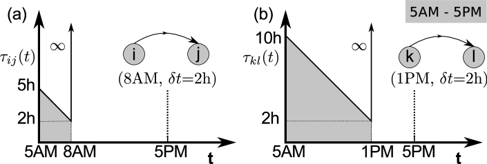
Figure 1: Schematic representation of the variation of temporal distances between two pairs of nodes, (a) $i$-$j$ and (b) $k$-$l$. The period of observation is between 5AM and 5PM. In panel (a), the two nodes are connected by an event that begins at 8AM and takes two hours to completion. In panel (b), the nodes are connected by an event of the same duration at 1PM. If the average temporal distance were defined only over its finite range, then $\tau_{ij}<\tau_{jk}$, although both pairs are connected via similar events.

Let us first take a look at option (i), averaging the temporal distance only over the period where it is finite. The problem with this approach is that it introduces a bias in favor of temporal paths taking place early within the period of observation. This can be illustrated with a simple example (see Fig.1): suppose that node $i$ directly interacts with $j$ only once at $t_{1}$, nodes $k$ and $l$ interact once at $t_{2}$, and no other temporal paths exist between these nodes. Here, $\tau_{ij}$ equals the shaded area divided by $t_{1}$ $(t_{2})$. Now, if $t_{1}\ll t_{2}$, the above averaging would imply that $\tau_{ij}\ll\tau_{kl}$, because when the distances are finite, $\tau_{ij}(t)\ll\tau_{kl}(t)\forall~{}t$.

On the basis of the above, we now set the following requirement for the average temporal distance $\tau_{ij}$: for any sequence of shortest temporal paths, the resulting average temporal distance should not depend on when that sequence takes place within the period of observation. Hence, $\tau_{ij}$ should be the same for both cases in Fig. 1. This leaves us with options (ii) and (iii). Both choices fulfill the above criterion for the simple example of Fig. 1. However, option (ii) can be ruled out by the following requirement: nodes that are not connected via a temporal path within the observation window should not become connected by applying the condition. If the entire event sequence is periodically repeated, this is not the case, as disconnected nodes may become connected via paths that may even span multiple window lengths. Thus, in order to avoid unnecessary artifacts to the extent that is possible, we base our definition of the average temporal distance on option (iii), where the finite period of observation is handled separately for each pair of nodes. Specifically, for calculating $\tau_{ij}$, we assume that if there is a temporal path between $i$ and $j$ which begins at $t=t_{1}$ and the period of observation is $[0,T]$, then this temporal path will reoccur at time $t=T+t_{1}$ without affecting the paths or distances between any other pair of nodes. It is easy to see that for the simple example of Fig. 1, this is analogous to assuming that we have a correct estimate of the frequency and duration of temporal paths between $i$ and $j$.

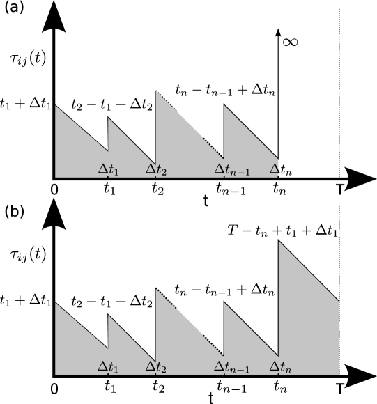
Figure 2: Schematic representation of the time variation of the temporal distance between a pair of nodes, $i$-$j$: (a) the actual distance and (b) the distance with periodic boundary condition on paths connecting $i$ and $j$.

Let us next have a closer look at how $\tau_{ij}(t)$ varies with time $t$ (see Fig. 2) in a setting where there are several shortest temporal paths at different points in time. Suppose that there is a temporal path along a time-ordered sequence of events starting at time $t_{1}$ through which one can reach node $j$ from $i$. If the time of completion of this path is $\Delta t_{1}$, then $\tau_{ij}(t_{1})=\Delta t_{1}$. If this is the only temporal path between $i$ and $j$ within the observation period, then for any $t<t_{1}$, $\tau_{ij}(t)=(t_{1}-t)+\Delta t_{1}$, and for any $t>t_{1}$, $\tau_{ij}(t)=\infty$. In general, if there are multiple shortest temporal paths between nodes $i$ and $j$ that begin at times $t_{1},\dots,t_{n}$ and have durations $\Delta t_{1},\dots,\Delta t_{n}$, respectively, then the temporal distance curve has the shape depicted in Fig. 2 (a). Application of the node-pair-specific boundary condition, i.e. repeating the first path, makes the temporal distance between nodes $i$ and $j$ behave as depicted in Fig. 2 (b). If there are $n$ shortest temporal paths between $i$ and $j$ within the observation period, with beginning times $t_{1},\dots,t_{n}$ and durations $\Delta t_{1},\ldots,\Delta t_{n}$, then the average temporal distance is given by

$$\begin{split}\tau_{ij}&=\frac{1}{T}\left[t_{1}\left(\frac{t_{1}}{2}+\Delta t_{1}\right)+\left(t_{2}-t_{1}\right)\left(\frac{t_{2}-t_{1}}{2}+\Delta t_{2}\right)\right.\\ &+\dots+(t_{n}-t_{n-1})\left(\frac{t_{n}-t_{n-1}}{2}+\Delta t_{n}\right)\\ &+\left.(T-t_{n})\left(\frac{T-t_{n}}{2}+t_{1}+\Delta t_{1}\right)\right].\end{split}$$ (1)

If there is only one temporal path between these nodes, the above equation reduces to $\tau_{ij}=\frac{T}{2}+\Delta t$, which is independent of the actual time of occurrence of the path, fulfilling the criterion that average temporal distance should be independent of the placement of the event sequence within the observation window.

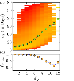
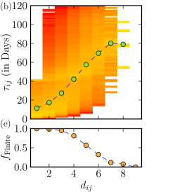
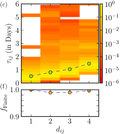
Figure 3: Top: the average temporal distance, $\tau_{ij}$, against the static graph distance, $d_{ij}$, between all pair of nodes for (a) the call network, (b) the e-mail network, and (c) the air transport network. The average temporal distances $\tau_{ij}$ were calculated using periodic boundary conditions, as detailed in the text. The colors represent the conditional probabilities of $\tau_{ij}$ for a given $d_{ij}$. Note the broad distribution of $P\left(\tau_{ij}|d_{ij}\right)$ in all three cases. Bottom: The fraction of finite temporal paths, $f_{\mathrm{Finite}}$, as a function of $d_{ij}$ for (d) the mobile phone call network, (e) the e-mail network and (f) the air transport network. It is seen that the longer a static path, the less likely the existence of a corresponding temporal path within the observation window.

II.2 An algorithm for calculating temporal distances

For calculating the above-defined average temporal distance between any two nodes $i$ and $j$ in an empirical event sequence, we need to detect the beginning times of all shortest temporal paths between $i$ and $j$ (i.e., $t_{1},\dots,t_{n}$, and the corresponding temporal distances at that particular time (i.e., $\tau_{ij}(t_{1})=\Delta t_{1},\dots,\tau_{ij}(t_{n})=\Delta t_{n}$). Here, we use the notion of vector clocks Mattern89 and propose an algorithm for efficient calculation of these quantities. For describing the algorithm, we use the metaphor of events transmitting information between nodes.

Let us assign a vector ${\boldsymbol{\phi_{i}}}$ for each node, such that its element $\phi_{i}^{j}(t)$ denotes the nearest point in time $t^{\prime}>t$ at which node $j$ can receive information transmitted from node $i$ at time $t$, either via a direct event or a time-ordered path spanned by any number of events. We also define $\phi_{i}^{i}(t)=t$. We then take advantage of a simple and efficient algorithm Lamport78 ; Mattern89 ; Kossinets08 to compute the shortest temporal paths between all nodes within a finite time period $[0,T]$. This is done by sorting the event list in the order of decreasing time (i.e. “backwards”) and going through the entire list of events once. Initially, we set all elements $\phi_{i}^{j}=\infty\forall i\neq j$ at $T$, indicating that no node can obtain any information, even indirectly, from any other after the end of our observation period $T$. Let us first assume that all events are instantaneous and undirected, i.e., information flows in both directions. We now go through the time-reversed event list event by event. For each event $(i,j,t)$ we compare the vector clocks of $i$ and $j$ element-wise, i.e., $\phi_{i}^{k}$ and $\phi_{j}^{k}$ $\forall k$, and update both with the lowest value. If $\phi_{i}^{k}$ is updated, this indicates that the event has given rise to a new shortest temporal path between $i$ and $k$ that begins at time $t$, and the associated temporal distance $\tau_{ik}(t)=\phi_{i}^{k}(t)-t$. As the event connects $i$ and $j$, we also set $\phi_{i}^{j}(t)=\phi_{j}^{i}(t)=t$, and thus $\tau_{ij}(t)=\tau_{ji}(t)=0$. As each update of the vector indicates the existence of a new temporal path, the updates define the beginning times $t_{1},\ldots,t_{n}$ and durations $\Delta t_{1},\ldots,\Delta t_{n}$ of temporal paths in the sum of Eq. 1, allowing for computing the average temporal distance between $i$ and $j$.

The algorithm can also be generalized for directed events with specific durations. For details, see Appendix A.

III Temporal paths and distances in empirical networks

III.1 Data description

In the following, we apply the above measures in the analysis of empirical data on temporal graphs. We have chosen two very different types of data sets: social networks, where information spreads through communication events in time, and an air transport network, where events transport passengers between airports. For each data set, we consider the respective temporal graph, i.e. the sequence of events, as well as its aggregated static counterpart where nodes are linked if an event joining them is observed in the sequence at any point in time.

Our first data set consists of time-stamped mobile phone call data over a period of 120 days Karsai10 , where each event corresponds to a voice call between two mobile phone users. We consider the events here as undirected and instantaneous, such that events may immediately transmit information. Note that although calls have in reality a duration, one person participates in one call only at a time, and thus for temporal paths, this duration can be neglected. For this study, we have selected a group of 1982 users that comprise the largest connected component (LCC) of an aggregated undirected network of users with a chosen zip code. Between these 1982 users, there are 5420 undirected edges, containing in total 153045 calls. This network is mutualized, i.e. we retain only events associated with links where there is at least one call both ways. Our second social network data set is an email network constructed from time-stamped email records of university users Eckmann04 within a period of 81 days. We consider emails as directed and study only the Largest Weakly Connected Component (LWCC) of the aggregated network, retaining events between its members, arriving at 2993 users connected by 28843 directed edges with 202687 emails. Third, we consider an air transport network, where the flights between all the airports in the US BTS for a period of 10 days between 14th and 23rd December 2008 are observed. The air transport network comprises 279 airports connected via 4152 directed edges and altogether 180192 flights; although edges are directed, 99.5% of them are reciprocated. In the static network, all airports belong to the Strongly Connected Component (SCC). All times are converted to GMT.

We note that for the two social networks, the observation periods (120 and 81 days) have been determined by the availability of data: we have chosen to use all the data available to us. For the air transport network, because of the inherent periodicity of flight schedules, a shorter window was chosen.

III.2 Relationship between temporal and static distances

Let us first consider the relationship between static and average temporal distances in the empirical systems, $d_{ij}$ in the aggregated network and $\tau_{ij}$ in the temporal graph (Fig. 3 a,b,c). Here, the static distance is defined as usual as the number of links along the shortest path connecting nodes in the aggregated network. For the call and email data sets, the average temporal distance can be considered as a measure of the time it takes for information to reach one node from another, if it is transmitted via calls or email such that recipients pass on the information. For the air transport network, the average temporal distance measures the average time to reach one airport from another, either directly or via connecting flights. In all cases, the static distance measures the number of links one has to traverse to get from one node to another. For a pair of nodes joined by such a path, the shortest temporal paths may of course follow another sequence of links, or not exist at all. One would still expect that in general, nodes that are far from each other in the static network would also have large temporal distances. For all three networks, we find that on average this is indeed the case (Fig. 3 a,b,c) – however, as the conditional distributions $P(\tau_{ij}|d_{ij})$ clearly show, there is surprisingly large variation around the average in all cases. As an example, in the mobile call network, there are node pairs that are at the same graph distance $d_{ij}$, but whose temporal distances differ by a factor of $10^{2}$. Likewise, one can find node pairs with a relatively short temporal distance that are either directly linked or 10 links apart in the static network. This highlights the importance of the temporal graph approach for processes whose dynamics depend on event sequences: e.g., for any spreading process on such systems, the pathways taken and the structure of the resulting branching tree can be entirely different if shortest temporal paths are followed.

For the social networks, the relationship between the static and average temporal distances is not linear, as there is an apparent increase in the slope for larger temporal distances. Furthermore, the fraction of node pairs at a given static distance that are also connected via a temporal path, $f_{\mathrm{Finite}}$, is seen to decrease for higher static distances (Fig. 3 d,e,f). Hence, in social communication networks, information between node pairs at large static distances may be on average transmitted only slowly or not at all. However, for the mobile call network, 95% of node pairs are nevertheless connected via a temporal path as very large static distances are infrequent; for the directed email network, the corresponding fraction is lower, 58%. Note that the behavior of $f_{\mathrm{Finite}}$ depends on the length of the observation period (120 days for the call network and 81 days for the email network), and, in general, the frequency of events. In addition, for the email network, the number of existing paths is naturally constrained by the directedness of the events, as from the point of view of information spreading, emails carry the information one way only, whereas calls may transfer information both ways. Thus, in the mobile call network, information may in theory be passed from almost any node to any other within the period of observation, whereas in the email network studied here this is not the case. Nevertheless, for both systems, an observation window spanning several months does not guarantee that all nodes are connected by a temporal path. On the contrary, reflecting its function and design, in the air transport network almost all pairs of nodes at any static distance are joined by a temporal path within the 10-day period of observation.

III.3 Effects of correlations on temporal distances

The empirical event sequences in our datasets that span the temporal paths contain correlations and heterogeneities affecting the temporal distances. First, events follow strong daily patterns. In the mobile call network, the call frequency shows a peak around lunch time and early evening (see Karsai10 ), whereas the frequency of flights is almost constant during the day. In the night, calls and departures of flights are infrequent. Second, in addition to the daily pattern, there are other non-uniformities in the event sequence: especially in human communications, bursty behavior giving rise to broad distributions of inter-event times is common Barabasi10 ; WuPNAS2010 ; Karsai10 . Third, there are event-event correlations, where one event may trigger another one, or events have been scheduled such that one follows another. Such correlations give rise to short waiting times between consecutive events along temporal paths.

The effects of heterogeneities and correlations on temporal distances can be investigated by applying null models where the original event sequences are randomized to systematically remove these correlations Holme05a ; Karsai10 . Here, we apply null models that separately destroy the following correlations: bursty or periodic event dynamics on single links, event-event correlations between links and, and the daily patterns. All structural properties of the static network are retained, as the null models only modify the times of events between nodes. The null models are as follows: (i) In the equal-weight link-sequence shuffled model, whole single-link event sequences are randomly exchanged between links having the same number of events. Event-event correlations between links are destroyed. (ii) In the time-shuffled model, the time stamps of the whole event sequence are shuffled. In this case, the bursts, periodicity and the event-event correlations are destroyed, while the daily patterns are retained. (iii) In the random-time model, the time stamps of all the events are chosen uniformly randomly from the period of observation. Here, all temporal correlations including the daily cycle are destroyed. When the events have a duration $\delta t$, this value remains attached to each event whenever the time of its occurrence changes.

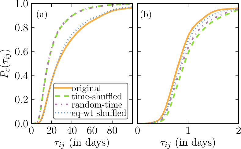
Figure 4: Cumulative distribution of the temporal distances for the (a) mobile phone call and (b) air transport network. The corresponding distribution for the time-shuffled, random-time and equal-weight link-sequence shuffled cases are also shown. It is seen that the distances in the mobile phone call network are relatively long compared to the time-shuffled and random references, whereas they are short in the air transport transport network designed to transfer passengers in an optimal way.

It has been earlier seen for the full mobile communication network that the burstiness of event sequences results in slower speed of SI dynamics Karsai10 . This observation was based on simulated spreading, averaged over a number of initial conditions. As such dynamics follows shortest temporal paths, one would expect a similar effect on average temporal path lengths in general. This is indeed the case. Fig. 4(a) shows the cumulative probability distribution (CDF) of temporal distances for the original sequence and null models. Clearly, distances are shorter for the time-shuffled and random-time models where bursts are destroyed; the similarity of these curves points out that the daily pattern plays a negligible role. The similarity of the CDF’s for the original sequence and equal-weight link-sequence shuffled model indicates that event-event correlations are also fairly unimportant for temporal distances, in line with Karsai10 .

For the air transport network, the situation is strikingly different [Fig. 4(b)]. The temporal distances in the original case are lower than for any null model, indicating that overall, the role of heterogeneities and correlations is to speed up dynamics in this system. This is not surprising as the events of this transport network are scheduled in an optimized way for the network to efficiently transport passenger. Removing event-event correlations (the equal-weight link-sequence shuffled model) is seen to slightly increase distances. The daily pattern is also seen to give rise to a minor increase in distances.

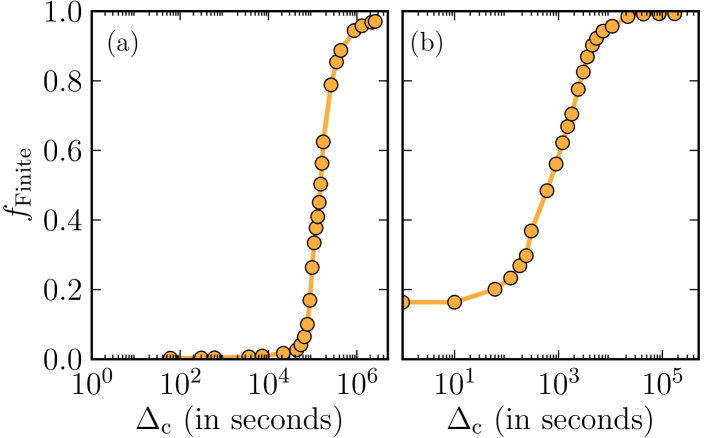
Figure 5: Fraction of finite temporal paths as a function of $\Delta_{\mathrm{c}}$ for the (a) mobile phone call and (b) air transport network.

III.4 Temporal paths with waiting time cutoff

So far, we have considered any sequence of events that follows temporal ordering a valid path. Let us now introduce an additional criterion for the existence of a path: the waiting time cutoff $\Delta_{\mathrm{c}}$, indicating the maximum allowed time between two consecutive events on a path. As an example, suppose there is an instantaneous event between nodes $i$ and $j$ at time $t_{1}$, and another between $j$ and $k$ at time $t_{2}$. These events then span the path $i\rightarrow j\rightarrow k$ only if the time difference between the events $0<(t_{2}-t_{1})\leq\Delta_{\mathrm{c}}$. If the events have an associated duration $\delta t$, the criterion becomes $0<\left[t_{2}-\left(t_{1}+\delta t_{1}\right)\right]\leq\Delta_{\mathrm{c}}$. If spreading dynamics along such paths are considered, the cutoff makes such dynamics SIR-like. In the SIR dynamics (Susceptible, Infectious, Recovered), an infectious node remains infectious only for a limited period of time before recovery and immunity to further infections. Hence, in such dynamics, for anything to be transmitted via a node, it has to be transmitted quickly enough. In the context of mobile calls, the cutoff time means that information is no longer passed on after a too long waiting time, i.e. it becomes obsolete or uninteresting. Similarly, for the air transport network, imposing a cutoff means that flights are not considered as connecting if the transit time is too long. Temporal paths constrained by the waiting time cutoff are the paths along which such spreading or transport processes may take place.

The cutoff time $\Delta_{\mathrm{c}}$ restricts the number of allowed paths, and we quantify this effect by calculating the overall fraction of node pairs joined by finite temporal paths within the period of observation, $f_{\mathrm{Finite}}$, also called the reachability ratio Holme05a , as a function of $\Delta_{\mathrm{c}}$. In the call network, for low $\Delta_{\mathrm{c}}$, most nodes remain disconnected [Fig. 5(a)]. However in the air transport network, even when $\Delta_{\mathrm{c}}=$1 sec, $f_{\mathrm{finite}}=0.16$. This is because of two factors: a large number of direct connections, and a large number of simultaneous arrivals and departures at airports. For both networks, most pairs of nodes are eventually connected by temporal paths as $\Delta_{\mathrm{c}}$ increases. For the call network, connectivity emerges approximately when $\Delta_{\mathrm{c}}>2$ days. Hence for any information to percolate through this system, nodes should forward it for at least 2 days after its reception. This result is fairly surprising; such a long period severely constrains global information cascades. However, it is in line with earlier observations that in simulations, structural and temporal features of call networks tend to limit the flow of information Onnela07 ; Karsai10 . For the air transport network, most temporal paths become finite when $\Delta_{\mathrm{c}}>30$ minutes. This is consistent with the minimum transit time required for catching a connecting flight.

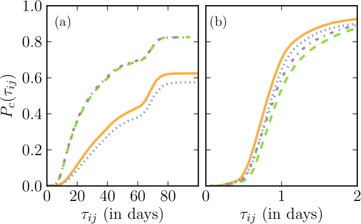
Figure 6: Comparison of the cumulative probability distributions of the temporal distances for the original and the randomized null models in the (a) mobile phone call network with a cutoff $\Delta_{c}=2$ days and (b) air transport network with cutoffs $\Delta_{c}^{\mathrm{min}}$ = 30 min and $\Delta_{c}$ = 5 hours. Line styles denote different null models, similarly to Fig. 4.

Let us next apply the null models and study temporal paths with cutoffs $\Delta_{\mathrm{c}}$. For the call network [Fig. 6 (a)], we set $\Delta_{\mathrm{c}}=$ 2 days. The CDFs of temporal distances show that only a fraction of finite temporal paths exists for all cases. This fraction is considerably larger for the time-shuffled and random-time null models, as the bursty event sequences give rise to longer waiting times and thus limit the number of existing paths. In addition, as above, the temporal distances for these null models are on average lower than for the original sequence, and hence also SIR-like dynamics is slowed down by bursts. Further, event-event correlations, i.e., rapid chains of calls $i\rightarrow j\rightarrow k$, make the paths somewhat faster, as could be expected, since in the equal-weight link-sequence shuffled model where such chains are destroyed the temporal distances are higher. The jump in the tail of the distribution is due to the finite 120-day period of observation and a large number of pairs of nodes connected via two events only, giving an average $t_{ij}\approx 60$ days.

For the air transport network, we apply an additional lower waiting time cutoff to account for the time needed to catch a connecting flight, and require the waiting times of between consecutive events to be between $\Delta_{\mathrm{c}}^{\mathrm{min}}$ = 30 min and $\Delta_{\mathrm{c}}$ = 5 hrs. The order of the cumulative probability distributions of temporal distances [Fig. 6 (b)] for all the null models is similar to the unconstrained case. Like for the call network, event-event correlations are seen to shorten temporal paths, as destroying them with the equal-weight link-sequence shuffled model gives rise to longer distances.

III.5 Temporal Closeness Centrality

So far, we have focused on the overall temporal distances that limit the speed of any dynamics on temporal graphs. To conclude our investigation, let us focus on the properties of individual nodes and their importance. To measure of how quickly all other nodes can be reached from a given node, we define the temporal closeness centrality as

$$C_{i}^{\mathrm{T}}=\frac{1}{N-1}\sum_{j}\frac{1}{\tau_{ij}},$$ (2)

where $\tau_{ij}$ is the average temporal distance between $i$ and $j$ and $N$ the number of nodes. A high value of $C_{i}^{\mathrm{T}}$ thus indicates that other nodes can be quickly reached from $i$. This measure is a generalization of the closeness centrality for static networks, defined as the inverse of the average length of the shortest paths to all the other nodes in the graph Freeman79 :

$$C_{i}^{\mathrm{S}}=\frac{1}{N-1}\sum_{j}\frac{1}{d_{ij}},$$ (3)

where $d_{ij}$ is the static distance between the nodes $i$ and $j$. A high value of $C_{i}^{\mathrm{S}}$ indicates that in the static network other nodes can be reached in a few steps from $i$, whereas low value means that other nodes are on average either unreachable or can only be reached via long paths.

For comparing the static and temporal closeness centrality to topological properties of nodes, we adopt the point of view of spreading, where short distances to other nodes are likely to improve the efficiency of the process, and central nodes are likely to be influential spreaders. We study the dependence of the static and temporal closeness centrality of a node on two quantities: node degree $k$ and its $k$-shell index, $k^{s}$. The node degree can be viewed as a first approximation of the importance of a node for spreading. However, it has recently been shown that in fact, the most efficient spreaders are located within the core of the network, i.e. have a high value of $k^{s}$ Kitsak10 . The $k$-shell index of a node is an integer quantity, measuring its “coreness”. To decompose the network into its $k^{s}$-shells, all nodes with degree $k=1$ are recursively removed until no more such nodes remain, and assigned to the 1-shell. Remaining higher-degree nodes are then recursively removed for each value of $k$ and assigned to the corresponding shell, until no more nodes remain.

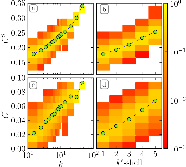
Figure 7: Static and temporal closeness centrality ($C^{\mathrm{S}}$ and $C^{\mathrm{T}}$) of the nodes against their (a,c) degree, $k$ and (b,d) $k^{s}$-shell index in the mobile phone call network. Circles denote mean values, while the shading represents conditional probabilities $P(C^{\mathrm{S,T}}|k)$ and $P(C^{\mathrm{S,T}}|k^{s})$.

The dependence of the static and temporal closeness centrality for the call network on both $k$ and $k^{s}$ is shown in Fig. 7. Clearly, both quantities $C^{\mathrm{S}}$ and $C^{\mathrm{T}}$ increase with $k$ and $k^{s}$ on average. However, again there is a large spread around the mean, and nodes with a high $k$ or $k$-shell index but a low static or temporal closeness can be found. Measured with the linear Pearson correlation coefficient, we find that the static $C^{\mathrm{S}}$ correlates with $k$ and $k^{s}$ with coefficient values of $C=0.80$ and $C=0.81$, respectively. The correlation of the temporal $C^{\mathrm{T}}$ with $k$ and $k^{s}$ is slightly weaker, with values of $C=0.69$ and $C=0.76$, respectively. However, even these values are fairly high. Thus both the static and temporal closeness centralities are clearly associated with high degrees and shell indices on average.

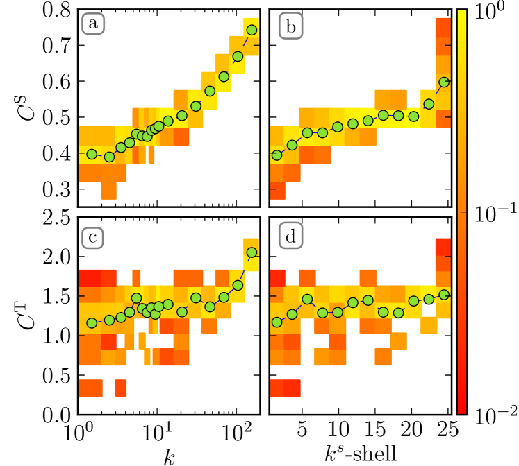
Figure 8: Static and temporal closeness centrality ($C^{\mathrm{S}}$ and $C^{\mathrm{T}}$) of the nodes against their (a,c) degree, $k$ and (b,d) $k^{s}$-shell index in the air transport network. Circles denote mean values, while the shading represents conditional probabilities $P(C^{\mathrm{S,T}}|k)$ and $P(C^{\mathrm{S,T}}|k^{s})$.

For the air transport network, we find a different result (Fig. 8). The static closeness centrality $C^{\mathrm{S}}$ correlates strongly with degree $k$ ($C=0.89$) and the $k^{s}$-shell index ($C=0.88$). However, the correlation between the temporal closeness centrality with $k$ and $k^{s}$ is much weaker, with coefficient values $C=0.45$ and $C=0.46$, respectively. The explanation for this observation is that the network is geographically embedded, and temporal path lengths are heavily influenced by flight times, i.e. the geographical distances between airports. Thus the nodes representing airports around the central regions of USA should on average be connected to other airports by short temporal paths, unless connected by a too low frequency of flights, whereas airports around the coastal areas should have lower temporal centralities. Indeed, this is the case. When ranked according to $C^{\mathrm{T}}$, the top three airports are ATL, Atlanta (rank=1, $k$=156, $k^{s}$=25); ORD, Chicago (rank=2, $k$=133, $k^{s}$=25); DFW, Dallas (rank=3, $k$=126, $k^{s}$=25). These major airports have high values of $k$ and $k^{s}$, reducing the number of transfers needed to reach other airports, and are located away from the coast. There are also airports that have a high temporal centrality but low $k$ and $k^{s}$, typically located in the central states of USA and also connected to other temporally central nodes, e.g., CHA, Chattanooga (rank=8, $k$=5, $k^{s}$=5); MGM, Montgomery (rank=9, $k$=2, $k^{s}$=2); ACT, Waco (rank=10, $k$=1, $k^{s}$=1). On the contrary, many interlinked coastal hubs that score low in the temporal centrality ranking can be found in the highest $k^{s}$-shells: e.g., IAD, Washington (rank=152, $k$=64, $k^{s}$=25); MCO, Orlando (rank=79, $k$=69, $k^{s}$=25); JFK, New York (rank=199, $k$=59, $k^{s}$=25).

IV Conclusions and Discussion

The properties of time-ordered temporal paths play a crucial role for any dynamics taking place on temporal graphs, such as the flow of information or resources or epidemic spreading. In essence, their maximum velocity is defined by the time it takes to complete such paths. Building on a definition of average temporal distance and its algorithmic implementation, we have studied temporal paths in empirical networks. Although our results show that temporal and static distances between nodes are correlated, in general there is a wide spread. Thus although nodes may be close in the static network, the time it takes to reach one from another may be very long, or vice versa, and in some cases, there is no temporal path at all. Because of this, any spreading process may follow very different paths on the temporal graph, and nodes that appear fairly insignificant from the static network perspective may in fact rapidly transmit information or disease around the network. Second, as shown with null models, temporal distances are affected by heterogeneities and correlations in the sequence of events spanning the paths. In line with earlier observations, these were seen to increase temporal distances for human communication networks – however, for the air transport network, the optimized scheduling of flights has the opposite effect.

Furthermore, we have also raised the issue of the finite observation period. For any measure to be applied on temporal graphs, the size and finiteness of the time window are important issues. Here, we have taken care to define the average temporal distance such that unnecessary artifacts are avoided. Yet, the application of this measure may yield results that are not useful if the observation window is too short in relation to event frequency. On the other hand, if the observation window is too long, the system may undergo changes during the window (e.g. in terms of its node composition) that make the results difficult to interpret. Hence, for any analysis of temporal graphs, the observation window issue is an important one, and further studies and methods for choosing a proper window size are in our view called for.

Finally, it is worth stressing that the null models we apply retain both the underlying network topology as well as the total numbers of events on each of its edges; hence, depending on the temporal heterogeneities, the dynamics of processes may differ a lot even when they take place on networks that appear similar from the static perspective. This is especially crucial for processes such as SIR spreading, where infection may not be transmitted further if the waiting times between consecutive events on temporal paths are too long. Thus, in simulations and modeling of processes such as epidemic spreading, information flow, and socio-dynamic processes in general, the time-domain properties of the event sequences that carry the interactions should be taken into account.

Appendix A Algorithm for computing temporal distances

Figure 9: Pseudo code for the temporal distance algorithm with directed and non-instantaneous events.

Here we present the generalized temporal distance algorithm, where the events are directed and/or have a duration to completion. The main flow of the algorithm follows the instantaneous and undirected case, see Sect. II. However, when the events are directed, for each event $(i,j,t)$ only the vector clock of $i$ is compared element-wise with that of $j$, i.e., $\phi_{i}^{k}$ and $\phi_{j}^{k}$ $\forall k$. If $\phi_{j}^{k}<\phi_{j}^{k}$, $\phi_{i}^{k}$ is replaced with $\phi_{j}^{k}$, and we also set $\phi_{i}^{j}(t)=t$. The vector clock of $j$ remains unchanged. When the events also have an associated duration $\delta t$, we have to define an additional vector for each node, $\boldsymbol{\psi}_{i}$, which stores the last observed beginning times of temporal paths from $i$ to all other nodes. Like for ${\boldsymbol{\phi_{i}}}$, the elements of this vector are also set to $\infty$ in the beginning of a run. When handling an event $(i,j,t,\delta t)$, the vector clock of $i$ is again element-wise compared to that of $j$, and if $\phi_{i}^{k}<\phi_{j}^{k}$ for some $k$, it is checked if $\psi_{j}^{k}>t+\delta t$. If this condition holds, the element $\phi_{i}^{k}$ is updated to $\phi_{j}^{k}$ and the element $\psi_{i}^{k}=t$. One also sets $\phi_{i}^{j}(t)=t+\delta t$ and $\psi_{i}^{j}(t)=t$, since $j$ can be reached from $i$ through an event starting at $t$ and finishing at $t+\delta t$, and thus $\tau_{ij}(t)=\delta t$. A pseudo-code for the algorithm is given below.