Chebyshev matrix product state approach for spectral functions

Abstract

We show that recursively generated Chebyshev expansions offer numerically efficient representations for calculating zero-temperature spectral functions of one-dimensional lattice models using matrix product state (MPS) methods. The main features of this Chebychev matrix product state (CheMPS) approach are: (i) it achieves uniform resolution over the spectral function’s entire spectral width; (ii) it can exploit the fact that the latter can be much smaller than the model’s many-body bandwidth; (iii) it offers a well-controlled broadening scheme that allows finite-size effects to be either resolved or smeared out, as desired; (iv) it is based on using MPS tools to recursively calculate a succession of Chebychev vectors $|t_{n}\rangle$, (v) whose entanglement entropies were found to remain bounded with increasing recursion order $n$ for all cases analyzed here; (vi) it distributes the total entanglement entropy that accumulates with increasing $n$ over the set of Chebyshev vectors $|t_{n}\rangle$, which need not be combined into a single vector. In this way, the growth in entanglement entropy that usually limits density matrix renormalization group (DMRG) approaches is packaged into conveniently manageable units. We present zero-temperature CheMPS results for the structure factor of spin-$\frac{1}{2}$ antiferromagnetic Heisenberg chains and perform a detailed finite-size analysis. Making comparisons to three benchmark methods, we find that CheMPS (1) yields results comparable in quality to those of correction vector DMRG, at dramatically reduced numerical cost; (2) agrees well with Bethe Ansatz results for an infinite system, within the limitations expected for numerics on finite systems; (3) can also be applied in the time domain, where it has potential to serve as a viable alternative to time-dependent DMRG (in particular at finite temperatures). Finally, we present a detailed error analysis of CheMPS for the case of the noninteracting resonant level model.

I Introduction

Consider a one-dimensional lattice model amenable to treatment by the density matrix renormalization group (DMRG),white:dmrg1 ; white:dmrg2 ; Schollwock2005 ; Schollwoeck2010 with Hamiltonian $\hat{H}$, ground state $|0\rangle$ and ground state energy $E_{0}$. This paper is concerned with zero-temperature spectral functions of the form

$$\mathcal{A}^{\mathcal{BC}}(\omega)=\langle{0}|\hat{\mathcal{B}}\,\delta(\omega-\hat{H}+E_{0})\,\hat{\mathcal{C}}|{0}\rangle\;,$$ (1)

which represents the Fourier transform $\int\frac{dt}{2\pi}e^{i\omega t}G^{\mathcal{BC}}(t)$ of the correlator

$$G^{\mathcal{BC}}(t)=\langle 0|\hat{\mathcal{B}}(t)\hat{\mathcal{C}}(0)|0\rangle\;.$$ (2)

One possible framework for calculating such spectral functions is to expand them in terms of Chebychev polynomials, as advocated in Ref. Weisse2006, . Such a Chebyshev expansion offers precise and convenient control of the accuracy and resolution with which a spectral function is to be computed. This is very useful, particularly when broadening the spectral function of a length-$L$ system, which exhibits finite-size subpeaks with spacing $\omega_{L}\sim 1/L$, in order to mimick that of an infinite system: if the latter has structures (e.g. sharp or diverging peaks) which are not yet properly resolved at the scale $\omega_{L}$, the broadened version of the finite-size spectral function inevitably bears $L$-dependent errors in the vicinity of these structures. Hence, when calculating the finite-size version of these structures for the length-$L$ system, there is no need to achieve an accuracy beyond that of the expected $L$-dependent errors, and having convenient control of this accuracy can significantly reduce numerical costs.

In this paper, we show that Chebyshev expansions offer numerically efficient representations for calculating spectral functions using matrix product state (MPS) methods,dukelsky1998 ; Vidal2004 ; verstraete:dmrg-pbc ; Verstraete2004b ; McCulloch2007 ; Schollwoeck2010 with numerical costs that compare favorably to those of other established DMRG-based approaches. In particular, the Chebychev MPS approach presented here, to be called CheMPS, allows the abovementioned control of accuracy and resolution to be imported into the DMRG/MPS arena.

The historically first approach for calculating spectral functions with DMRG is the continued-fraction expansion.Hallberg1995 While this method requires only modest numerical resources, it is limited to low frequencies and it is difficult to produce reliable results with it in the case of continua (however, algorithmic improvements were reported recently). At present, the most accurate, but also most time-consuming approaches are: (i) the correction vector (CV) method,RamaseshaPatiKrishnamurthyShuaiBredas1997 ; Kuhner1999 ; Jeckelmann2002 and (ii) time-dependent DMRG (tDMRG),Vidal2004 ; White2004 ; DaleyKollathSchollwoeckVidal2004 ; Verstraete2004b ; Schmitteckert2004 in particular when combined with linear prediction techniques.PressTeukolskyVetterlingFlannery2007 ; PereiraWhiteAffleck2008 ; WhiteAffleck2008 ; BarthelSchollwoeckWhite2009 Since any new approach must measure up to their standards, let us briefly summarize their key ideas, advantages and drawbacks.

(i) To calculate $\mathcal{A}^{\mathcal{BC}}(\omega)$ using the CV approach, it is expressed as

$$\mathcal{A}^{\mathcal{BC}}(\omega)=\langle 0|\hat{\mathcal{B}}|\mathcal{C}\rangle_{\omega}\;,$$ (3a)

in terms of the so-called correction vector

$$|\mathcal{C}\rangle_{\omega}\equiv-\lim_{\eta\to 0}\frac{1}{\pi}{\rm Im}\left[\frac{1}{\omega-\hat{H}+E_{0}+i\eta}\right]\hat{\mathcal{C}}|0\rangle\;.$$ (3b)

The correction vector can be calculated (for finite broadening parameter $\eta$) using either conventional DMRG RamaseshaPatiKrishnamurthyShuaiBredas1997 ; Kuhner1999 ; Jeckelmann2002 or variational matrix product state (MPS) methods.Weichselbaum2009 A major advantage of this approach is that arbitrarily high spectral resolution can be achieved by reducing $\eta$ and sampling enough frequency points. However, this comes at considerable numerical costs: first, a separate calculation is required for every choice of $\omega$ (though in doing so, results for $|\mathcal{C}\rangle_{\omega}$’s from previous frequencies can be incorporated); and second, the calculation of $|\mathcal{C}\rangle_{\omega}$ involves an operator inversion problem that is numerically poorly conditioned, ever more so the smaller $\eta$ is.

(ii) An alterative possibility is to use tDMRG to calculate the time-domain correlator $G^{\mathcal{BC}}(t)$, Fourier transforming to the frequency domain only at the very end. To this end, one expresses

$$G^{\mathcal{BC}}(t)=e^{iE_{0}t}\langle 0|\hat{\mathcal{B}}|\tilde{\mathcal{C}}\rangle_{t}\;$$ (4a)

in terms of the time-evolved state

$$|\tilde{\mathcal{C}}\rangle_{t}\equiv e^{-i\hat{H}t}\hat{\mathcal{C}}|0\rangle\;$$ (4b)

and uses tDMRG to calculate the latter. Two attractive features of this strategy are: first, it builds on an extensive body of algorithmic knowledge for efficiently calculating time-evolution;Vidal2004 ; White2004 ; DaleyKollathSchollwoeckVidal2004 and second, a simple linear-prediction scheme PressTeukolskyVetterlingFlannery2007 ; PereiraWhiteAffleck2008 ; WhiteAffleck2008 ; BarthelSchollwoeckWhite2009 can be used to extrapolate the time-dependence calculated for short and intermediate time scales to longer times, thereby improving the quality of results at low frequency at hardly any additional numerical cost. However, obtaining reliable results over a sufficiently large time interval can, in itself, be numerically very expensive, since the time-evolution of the many-body state $|\tilde{\mathcal{C}}\rangle_{t}$ is accompanied by a strong growth in entanglement entropy. This unavoidably also implies a growth of tDMRG truncation errors.

Note that in both of the schemes outlined above, significant (often heroic) amounts of numerical resources are devoted to calculating a single state, $|\mathcal{C}\rangle_{\omega}$ for given $\omega$ or $|\tilde{\mathcal{C}}\rangle_{t}$ for given $t$, as accurately as possible; the overlaps or expectation values of interest, namely $\langle 0|\hat{\mathcal{B}}|\mathcal{C}\rangle_{\omega}$ for $\langle 0|\hat{\mathcal{B}}|\tilde{\mathcal{C}}\rangle_{t}$, are only calculated at the end, in a single, final step, after $|\mathcal{C}\rangle_{\omega}$ or $|\tilde{\mathcal{C}}\rangle_{t}$ have been fully determined. Actually, these states are calculated so accurately that they would have been equally suitable for calculating any other quantity (correlator or matrix element) involving that state. In a sense, DMRG is asked to work harder than necessary: it is used to calculate a single state with “general-purpose accuracy”, whereas the accurate calculation of a particular expectation value involving that state would have been sufficient.

The main motivation for the present work is to attempt to reduce this calculational overhead by employing a representation of the spectral function that avoids the need for calculating a single state with such high accuracy and instead allows numerical resources to be focussed directly on the calculation of the relevant expectation values. This can be achieved by representing the spectral function via a Chebychev expansion,Wheeler1974 ; SilverRoeder1994 ; Weisse2006 whose coefficients, the so-called Chebyshev moments, can be calculated recursively using MPS tools. Below, we briefly summarize the structure and main features of such an expansion, thereby providing both an introduction and an overview of the material developed in detail in the main part of this paper.

The Chebychev polynomials $T_{n}(x)$ form an orthonormal set of polynomials on the interval $x\in[-1,1]$. They are very well studied mathematically,AbramowitzStegun1970 ; Boyd1989 ; Rivlin1990 and are widely used for function expansions since they have very favorable convergence properties. As will be described in detail below, the spectral function can be represented approximately by a so-called Chebychev expansion, which becomes exact for $N\to\infty$, of the following form:

$$\mathcal{A}^{\mathcal{BC}}_{N}(\omega)=\frac{2W^{\prime}/W_{\!\ast}}{\pi\sqrt{1-\omega^{\prime 2}}}\left[g_{0}\mu_{0}+2\sum_{n=1}^{N-1}g_{n}\mu_{n}T_{n}(\omega^{\prime})\right].$$ (5)

Here the Chebyshev moments $\mu_{n}=\langle{0}|\hat{\mathcal{B}}|{t_{n}}\rangle$ are obtained from the Chebychev vectors $|{t_{n}}\rangle=T_{n}(\hat{H}^{\prime})\hat{\mathcal{C}}|{0}\rangle$, and the $g_{n}$ are known damping factors that influence broadening effects. The primes indicate that the Hamiltonian $\hat{H}$ and frequency $\omega$ were expressed in terms of rescaled and shifted versions, $\hat{H}^{\prime}$ and $\omega^{\prime}$, in such a manner that an interval $\omega\in[0,W_{\!\ast}]$ that contains the entire spectral weight is mapped onto a rescaled band $\omega^{\prime}\in[-W^{\prime},W^{\prime}]$ of halfwidth $W^{\prime}<1$.

This representation has several useful features:
(i) It resolves the interval $\omega\in[0,W_{\!\ast}]$ with a uniform resolution of $\mathcal{O}(W_{\!\ast}/N)$.
(ii) The range of frequencies over which the spectral function has nonzero weight, say ${W_{\!\!\mathcal{A}}}$ (to be called its spectral width) is often significantly smaller than the many-body bandwidth of the Hamiltonian, say $W$, as depicted in Fig 1.

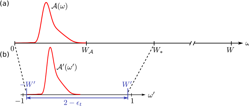
Fig. 1: (a) Sketch of a spectral function whose spectral width ${W_{\!\!\mathcal{A}}}$ is much smaller than the many-body bandwidth $W$. Before making a Chebychev expansion, we rescale the interval $\omega\in[0,W_{\!\ast}]$, with effective bandwidth $W_{\!\ast}=2{W_{\!\!\mathcal{A}}}$, onto the interval $\omega^{\prime}\in[-W^{\prime},W^{\prime}]$, shown in (b), with rescaled half-bandwidth $W^{\prime}=1-\frac{1}{2}\epsilon_{\rm t}$ and a safety factor $\epsilon_{\rm t}\simeq 0.025$.

By choosing the effective bandwidth $W_{\!\ast}$ to be of order ${W_{\!\!\mathcal{A}}}$ instead of $W$, huge gains in resolution are possible.
(iii) A well-controlled broadening scheme, encoded in the damping factors $g_{n}$, is available that allows finite-size effects to be either resolved or smeared out, as desired.
(iv) The Chebyshev vectors $|t_{n}\rangle$ are calculated using a (numerically stable) recursion scheme, which exploits Chebychev recurrence relations to calculate $|t_{n}\rangle$ from $H^{\prime}|t_{n-1}\rangle$ and $|t_{n-2}\rangle$ (see Eq. (30)). Thus, the expectation values from which the spectral function is constructed are built up in a series of recursive steps (see Eq. (7) below) instead of being calculated at the end in one final step.
(v) The bond entropy of successive Chebyshev vectors $|t_{n}\rangle$ is found empirically to remain bounded with increasing recursion number $n$, thus the complexity of these vectors remains managable up to arbitrarily large $n$.
(vi) Finally, and from the perspective of numerical costs, most importantly: CheMPS efficiently copes with the growth in bond entropy with increasing iteration number that usually limits DMRG approaches. It does so by distributing this entropy over all $|t_{n}\rangle$, thereby packaging it into managable units (see (v)). In particular, when constructing and using the states $|t_{n}\rangle$, one never needs to know more than three at a time (and after use may delete them from memory). Hence, it is not necessary to combine all information contained in all $|t_{n}\rangle$ into a single MPS.

Let us constrast this with the CV or tDMRG approaches: imagine expanding the correction vector or time-evolved state in terms of the Chebyshev vectors $|t_{n}\rangle$, i.e. expressing them as linear combinations of the form

$$|\mathcal{C}\rangle_{\omega}\simeq\sum_{n=0}^{N-1}C^{n}_{\omega}|t_{n}\rangle\;,\quad|\tilde{\mathcal{C}}\rangle_{t}\simeq\sum_{n=0}^{N-1}\tilde{C}^{n}_{t}|t_{n}\rangle\;,$$ (6)

respectively. (The coefficients $C^{n}_{\omega}$ and $\tilde{C}^{n}_{t}$ are related by Fourier transformation.) Now, the CV or tDMRG approaches in effect attempt to accurately represent the entire linear combination using a single MPS. This endevour is numerically very costly, since the entanglement entropy of this linear combination grows rapidly with $N$. The Chebychev approach avoids this problem by taking expectation values before performing the sum on $n$:

$$\langle 0|\hat{\mathcal{B}}|\hat{\mathcal{C}}\rangle_{\omega}\simeq\sum_{n=0}^{N-1}C^{n}_{\omega}\mu_{n}\;,\quad\langle 0|\hat{\mathcal{B}}|\tilde{\mathcal{C}}\rangle_{t}\simeq\sum_{n=0}^{N-1}\tilde{C}^{n}_{t}\mu_{n}\;.$$ (7)

Thus, the Chebychev expansion very conveniently organizes the calculation into many separate, and hence numerically less costly, packages or subunits.

Our paper is organized as follows. We introduce the Chebyshev expansion for spectral functions in sec:chebyshev-expansion and discuss its implementation using MPS including a new algorithm for performing a projection in energy in sec:mps-eval-coeffs. In sec:heisenberg we present CheMPS results for the structure factor of a spin-$\frac{1}{2}$ Heisenberg chains, perform a detailed analysis of finite-size effects (see fig:finite-size-analysis), and compare our results to CV, Bethe Ansatz and tDMRG (see Figs. 4, 6 and 8, respectively). In Sec. V we perform an extensive error analysis of the CheMPS approach using the quadratic resonant level model, and discuss some salient features of density matrix eigenspectra in Sec. VI. Section VII summarizes our main conclusions, and Sec. VIII presents a brief outlook towards possible future applications, involving time dependence or finite-temperature correlators. An Appendix gives a detailed account of CheMPS results for the resonant level model used for the error analysis of Sec. V.

II Chebyshev expansion of $\mathcal{A}^{\mathcal{BC}}(\omega)$

II.1 Chebyshev basics

Let us start by briefly summarizing those properties of Chebyshev polynomials that will be needed below. We follow the notation of Ref. Weisse2006, , which gives an excellent general discussion of Chebyshev expansion techniques (though without mentioning possible DMRG/MPS applications).

Chebyshev polynomials of the first kind, $T_{n}(x)$, henceforth simply called Chebyshev polynomials, are defined by the recurrence relations

$$\begin{split}T_{n+1}(x)&=2xT_{n}(x)-T_{n-1}(x),\\ T_{0}(x)&=1,\qquad T_{1}(x)=x\;.\end{split}$$ (8)

They also satisfy the useful relation (for $n\geq n^{\prime}$)

$$T_{n+n^{\prime}}(x)=2T_{n}(x)T_{n^{\prime}}(x)-T_{n-n^{\prime}}(x)\;.$$ (9)

Two useful explicit representations are:

$$T_{n}(x)=\cos\left[n\arccos(x)\right]=\cosh\left[n\,\textrm{arccosh}(x)\right].$$ (10)

On the interval $I=[-1,1]$ the Chebyshev polynomials constitute an orthogonal system of polynomials (over a weight function $(\pi\sqrt{1-x^{2}})^{-1}$), in terms of which any piecewise smooth and continuous function $\left.f(x)\right|_{x\in I}$ can be expanded. In fact, the $T_{n}(x)$ are optimally suited for this purpose, since they have the unique property (setting them apart from other systems of orthogonal polynomials) that on $I$ their values are confined to $|T_{n}(x)|\leq 1$, with all extremal values equal to $1$ or $-1$. This is evident from the first equality in Eq. (10); the second equality implies that for $x\notin I$, $|T_{n}(x)|$ grows rapidly with increasing $|x|$. These properties are illustrated in Fig. 2.

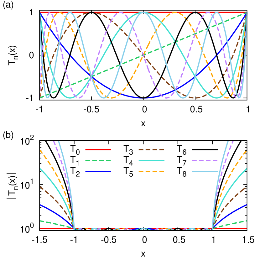
Fig. 2: (Color online) Chebyshev polynomials of the first kind, $T_{n}(x)$, for $n$ up to $8$. (a) All zeros and extrema of every $T_{n}(x)$ are located within the interval $I=[-1,1]$, and all extremal values equal $1$ or $-1$. (b) Chebyshev polynomials $|T_{n}(x)|$ for $x\in[-1.5,1.5]$. The $|T_{n>0}(x)|$ grow rapidly when $\left|{x}\right|$ increases beyond 1.

There are several ways of constructing Chebyshev approximations for $\left.f(x)\right|_{x\in I}$ (see Weisse et al.,Weisse2006 , Section II.A). The Chebyshev expansion that is practical for present purposes has the form

$$f(x) =\frac{1}{\pi\sqrt{1-x^{2}}}\left[\mu_{0}+2\sum_{n=1}^{\infty}\mu_{n}T_{n}(x)\right]\;,$$ (11)

where the Chebychev moments $\mu_{n}$ are given by

$$\mu_{n} =\int_{-1}^{1}dxf(x)T_{n}(x)\;.$$ (12)

An approximate representation of order $N$ is obtained for $f(x)$ if only the first $N$ terms (i.e. $n\leq N-1$) are retained. However, such a truncation in general introduces artificial oscillations, of period $\simeq 1/N$, called Gibbs oscillations. These can be smoothened by employing certain broadening kernels, which in effect rearrange the infinite series (11) before truncation. This leads to a reconstructed expansion of the form

$$f_{N}(x) =\frac{1}{\pi\sqrt{1-x^{2}}}\left[g_{0}\mu_{0}+2\sum_{n=1}^{N-1}g_{n}\mu_{n}T_{n}(x)\right]\;,$$ (13)

which (for properly chosen kernels) converges uniformly:

$$\max_{-1<x<1}|f(x)-f_{N}(x)|\stackrel{{\scriptstyle N\to\infty}}{{\longrightarrow}}0\;.$$ (14)

The reconstructed series (13) contains the same Chebyshev moments $\mu_{n}$ as Eq. (12), but they are multiplied by damping factors $g_{n}$, real numbers whose form is characteristic of the chosen kernel. Several choices have been proposed, which damp out Gibbs oscillations in somewhat different ways (see Ref. Weisse2006, for details). We will mostly employ Jackson damping, given by

$$g_{n}^{J}=\frac{(N-n+1)\cos\frac{\pi n}{N+1}+\sin\frac{\pi n}{N+1}\cot\frac{\pi}{N+1}}{N+1}.$$ (15)

This is usually the best choice, since it guarantees an integrated error of $\mathcal{O}(\frac{1}{N})$ for $f_{N}(x)$. When used to approximate a $\delta$-function $\delta(x-\bar{x})$ sitting at $\bar{x}\in I$, Jackson damping yields a nearly Gaussian peak of width $\sqrt{1-\bar{x}^{2}}\,\pi/N$. On one occasion we will also employ Lorentz damping,

$$g_{n,\lambda}^{L}=\frac{\sinh\left[\lambda\left(1-\frac{n}{N}\right)\right]}{\sinh\lambda},$$ (16)

where $\lambda$ is a real parameter. Lorentz damping preserves analytical properties (causality) of Green’s function and broadens a $\delta$-function $\delta(x-\bar{x})$ into a peak whose shape, for the choice $\lambda=4$ used here (following Ref. Weisse2006, ), is nearly Lorentzian, of width $\sqrt{1-\bar{x}^{2}}\,\lambda/N$.

To summarize: the order-$N$ Chebychev-reconstruction $f_{N}(x)$ with Jackson or Lorentzian damping with $\lambda=4$ yields a result that is very close to the broadened function

$$f^{X}_{N}(x)=\int_{-1}^{1}d\bar{x}K_{\eta^{\prime}_{N,\bar{x}}}^{X}(x-\bar{x})f(\bar{x})\;,$$ (17)

($X=J,L$) with broadening kernels and widths given by

$$K^{J}_{\eta^{\prime}}(x) = \frac{e^{-{x^{2}}/(2(\eta^{\prime 2})}}{\sqrt{2\pi}\eta^{\prime}}\;,\qquad\eta^{\prime}_{N,\bar{x}}=\sqrt{1-\bar{x}^{2}}\,\frac{\pi}{N}\;,\quad\phantom{.}$$ (18a)

$$K^{L}_{\eta^{\prime}}(x) = \frac{\eta^{\prime}/\pi}{x^{2}+{\eta^{\prime}}^{2}}\;,\qquad\eta^{\prime}_{N,\bar{x}}=\sqrt{1-\bar{x}^{2}}\,\frac{4}{N}\;,$$ (18b)

respectively. Thus, $f_{N}(x)$ resolves the shape of $f(x)$ with a resolution of $\mathcal{O}(1/N)$.

For purposes of illustration, fig:kernel-delta(a) shows three Chebyshev reconstructions of a $\delta$-function at $\bar{x}=0$: without damping, giving Gibbs oscillations; with Jackson damping, yielding a near-Gaussian peak; and with Lorentz damping, yielding a near-Lorentzian peak. Figure 3(b) shows a Jackson-damped Chebyshev reconstruction of a comb of Gaussian peaks $\sum_{\alpha}K^{J}_{\bar{\eta}^{\prime}_{\alpha}}(x-\bar{x}_{\alpha})$, whose widths $\bar{\eta}^{\prime}_{\alpha}$ are all equal. It illustrates how increasing $N$ reduces the amount of broadening until the original peak form is recovered for sufficiently large $N$. It also shows that the broadened peak widths depend on the peak positions, reflecting the fact that convolving a Gaussian of width $\bar{\eta}^{\prime}_{\alpha}$ with a near-Gaussian of width $\eta^{\prime}_{N,\bar{x}_{\alpha}}$ (Eq. (17)) produces a near-Gaussian of width

$$\eta^{\prime}_{\alpha}\simeq\sqrt{\bar{\eta}^{\prime 2}_{\alpha}+\eta^{\prime 2}_{N,\bar{x}_{\alpha}}}\;.$$ (19)

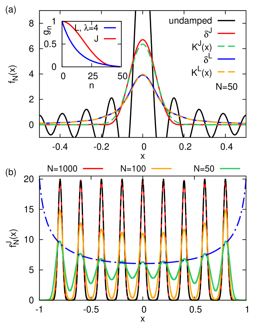
Fig. 3: Three Chebyshev reconstructions of $\delta(x)$, with $N=50$: the undamped case $(g_{n}=1)$ yields Gibbs oscillations (central peak has height $\delta_{50}(0)=16.23$); Jackson damping $(\delta^{J})$ mimicks a Gaussian peak $K^{J}(x)$ of width $\pi/N$; Lorentz damping ($\delta^{L}$) for $\lambda=4$ mimicks a Lorentzian peak $K^{L}(x)$ of width $\lambda/N$. Inset: Jackson and Lorentz damping factors, $g_{n}^{J}$ and $g_{n,\lambda=4}^{L}$, respectively, plotted for $N=50$. Both decrease monotonically from 1 to 0, but in somewhat different ways. (b) Jackson-damped reconstruction of a comb of normalized Gaussians (dashed line), all of width $\bar{\eta}^{\prime}=0.02$, for three values of $N$ (solid lines). The $x$-dependence of the peak heights is given by $[2\pi(\bar{\eta}^{\prime 2}+\eta^{\prime 2}_{N,x})]^{-1/2}$ (dash-dotted line), see Eq. (19).

To evaluate the $T_{n}(x)$ that occur in Eq. (13), we use the first equality of Eq. (10). Although numerically more efficient methods exist for this purpose,Weisse2006 their use becomes advisable only for expansion orders much larger than the $N\lesssim{\cal O}(10^{3})$ that we will need in this work.

II.2 Rescaling of $\omega$ and $\hat{H}$

To construct a Chebyshev expansion of the spectral function $\mathcal{A}^{\mathcal{BC}}(\omega)$ of Eq. (1), we need to rescale and shift Weisse2006 the Hamiltonian $\hat{H}\mapsto\hat{H}^{\prime}$ and the frequency $\omega\mapsto\omega^{\prime}$ in such a way that the spectral range of $\mathcal{A}(\omega)$, i.e. the interval $[0,{W_{\!\!\mathcal{A}}}]$ within which it has nonzero weight, is mapped into the interval $[-1,1]$. Rescaled, dimensionless energies and frequencies will always carry primes. As safeguards against “leakage” beyond $[-1,1]$ due to numerical inaccuracies, we choose the linear map (see Fig. 1)

$$\omega\in[0,W_{\!\ast}]\mapsto\omega^{\prime}\in[-W^{\prime},W^{\prime}]\;,\quad W^{\prime}=1-{\textstyle\frac{1}{2}}\epsilon_{\rm t}\;,\quad\phantom{.}$$ (20)

which entails two precautionary measures: first, the $\omega$-interval is taken to be larger than the requisite $[0,{W_{\!\!\mathcal{A}}}]$ by choosing the effective bandwidth $W_{\!\ast}$ to be larger than the spectral width ${W_{\!\!\mathcal{A}}}$; second, the $\omega^{\prime}$-interval is taken to be slightly smaller than the requisite $[-1,1]$ by choosing the rescaled half-bandwidth $W^{\prime}$ to be smaller than 1, with a safety factorWeisse2006 of $\epsilon_{\rm t}\simeq 0.025$. To be explicit, we define

$$\omega^{\prime} = \frac{\omega}{a}-W^{\prime}\;,\quad a=\frac{W_{\!\ast}}{2W^{\prime}}\;,$$ (21a)

$$\hat{H}^{\prime} = \frac{\hat{H}-E_{0}}{a}-W^{\prime}\;,$$ (21b)

where $\hat{H}^{\prime}$ has ground state energy $E_{0}^{\prime}=-W^{\prime}$. Then we express the spectral function (1) as

$$\mathcal{A}^{\mathcal{BC}}(\omega)=\frac{1}{a}\langle{0}|\hat{\mathcal{B}}\,\delta(\omega^{\prime}-\hat{H}^{\prime})\,\hat{\mathcal{C}}|{0}\rangle\;,$$ (22)

(with $\omega^{\prime}=\omega^{\prime}(\omega)$ and $\hat{H}^{\prime}$ given by Eqs. (21)), which by construction has no weight for $\omega^{\prime}\notin[-W^{\prime},W^{\prime}]$.

One possible choice for $W_{\!\ast}$ is to equate it to the width of the many-body spectrum of $H$, given by $W=E_{\rm max}-E_{0}$. When using DMRG, $E_{0}$ is usually already known from calculating the ground state $|{0}\rangle$ of $H$, and $E_{\rm max}$ can be found, e. g. , by calculating the ground state of $-H$ (reduced DMRG accuracy relative to usual ground state calculations is sufficient, since only $E_{\rm max}$ is of interest here.)

A disadvantage of the choice $W_{\!\ast}=W$ is that the many-body bandwidth $W$ typically is large (it scales with system size), whereas optimal spectral resolution requires $W_{\!\ast}$ to be as small as possible: since an $N$-th order Chebyshev expansion yields a resolution of $\mathcal{O}(1/N)$ on the interval $[-1,1]$, its resolution on the original interval $[0,W_{\!\ast}]$ will be $\mathcal{O}(W_{\!\ast}/N)$, which evidently becomes better the smaller $W_{\!\ast}$. If $\hat{\mathcal{B}}$ and $\hat{\mathcal{C}}$ are single-particle operators, the spectral width ${W_{\!\!\mathcal{A}}}$ of $\mathcal{A}^{\mathcal{BC}}(\omega)$ is independent of system size and hence much smaller than the many-body bandwidth $W$. In this case, it is advisable to choose $W_{\!\ast}$ to be of similar order (though still larger) than ${W_{\!\!\mathcal{A}}}$. We will choose $W_{\!\ast}=2{W_{\!\!\mathcal{A}}}$, which is typically $\ll W$, as illustrated in fig:rescaling-sketch.

II.3 Chebychev expansion in frequency domain

To expand the $\delta$-function in Eq. (22) in Chebyshev polynomials, we use $\hat{f}(x)=\delta(x-\hat{H}^{\prime})$ with $x=\omega^{\prime}$ in Eq. (12), and obtain from Eq. (13) a reconstructed Chebyshev operator expansion of the form:

$$\delta_{N}(\omega^{\prime}-\hat{H}^{\prime})=\frac{1}{\pi\sqrt{1-\omega^{\prime 2}}}\left[g_{0}+2\sum_{n=1}^{N-1}g_{n}T_{n}(\hat{H}^{\prime})T_{n}(\omega^{\prime})\right].$$ (23)

Inserting this into Eq. (22) for $\mathcal{A}^{\mathcal{BC}}(\omega)$ yields the Chebyshev expansion (5), with Chebyshev moments given by

$$\mu_{n} = \langle{0}|\hat{\mathcal{B}}T_{n}(\hat{H}^{\prime})\hat{\mathcal{C}}|{0}\rangle\;.$$ (24)

Thus $\mu_{n}$ is a ground state expectation value of an $n$-th order polynomial in $\hat{H}^{\prime}$, whose construction might a priori appear to become increasingly daunting as $n$ increases. Fortunately, this challenge can be dealt with recursively, by expressing the moments as

$$\mu_{n}=\langle{0}|\hat{\mathcal{B}}|{t_{n}}\rangle\;,\qquad|{t_{n}}\rangle=T_{n}(\hat{H}^{\prime})\hat{\mathcal{C}}|{0}\rangle,$$ (25)

and calculating the Chebyshev vectors $|{t_{n}}\rangle$ by exploiting the Chebyshev recurrence relations (8). The details of this recursive scheme will be discussed in Section III.

II.4 Chebychev expansion in time domain

The Chebyshev expansion can also be employed for studying time evolution in general, and the correlator $G^{\mathcal{BC}}(t)$ in particular. To this end, we express the time-evolution operator as

$$\hat{U}(t) = e^{-i\hat{H}t}=\int_{-1}^{1}d\omega^{\prime}e^{-i\left[a(\omega^{\prime}+W^{\prime})+E_{0}\right]t}\delta(\omega^{\prime}-\hat{H}^{\prime})\;,\qquad\phantom{.}$$ (26)

and insert Eq. (23) (without damping, $g_{n}=1$) into the latter. This yieldsTal-Ezer1984 ; Leforestier1991

$$\hat{U}_{N}(t) = e^{-i(E_{0}+aW^{\prime})t}\left[c_{0}(t)+2\sum_{n=1}^{N-1}T_{n}(\hat{H}^{\prime})c_{n}(t)\right]\!\!,\qquad\phantom{.}$$ (27a)

$$c_{n}(t) = \int_{-1}^{1}\frac{e^{-iat\omega^{\prime}}T_{n}(\omega^{\prime})}{\pi\sqrt{1-\omega^{\prime 2}}}d\omega^{\prime}=(-i)^{n}J_{n}(at)\,.$$ (27b)

Here $J_{n}(at)$ is the Bessel function of the first kind of order $n$. It decays very rapidly with $n$ once $n>at$. Hence, an expansion of given order $N$ gives an essentially exact representation of $\hat{U}(t)$ for times up to $t_{\rm max}\lesssim\frac{N}{a}$, while $c_{N-1}(t)$ provides an estimate of the error.

Inserting Eqs. (27) into Eqs. (4) for $G^{\mathcal{BC}}(t)$ we find

$$G_{N}^{\mathcal{BC}}(t)=e^{-iaW^{\prime}t}\left[\mu_{0}J_{0}(at)+2\sum_{n=1}^{N-1}(-i)^{n}\mu_{n}\,J_{n}(at)\right],$$ (28)

where the Chebyshev moments $\mu_{n}$ are again given by Eq. (25). Thus the Chebyshev expansions of $G^{\mathcal{BC}}(t)$ and $\mathcal{A}^{\mathcal{BC}}(\omega)$ are governed by the same set of moments $\mu_{n}$, as is to be expected for functions linked by Fourier transformation.

III MPS evaluation of the Chebyshev moments $\mu_{n}$

We now present a recursive scheme for calculating the Chebyshev moments $\mu_{n}$. The manipulations described below were implemented using MPS-based methods,dukelsky1998 ; Vidal2004 ; verstraete:dmrg-pbc ; Verstraete2004b ; McCulloch2007 ; Schollwoeck2010 which are very convenient for constructing the states of interest, while matrix-product operatorsMcCulloch2007 (MPOs) simplify the implementation of the shift- and rescaling transformation eq:cheby-h-rescaled of the Hamiltonian.

III.1 Recurrence fitting

To initialize the Chebyshev expansion, we calculate ground state $|{0}\rangle$ and ground state energy $E_{0}$ of $\hat{H}$, make a specific choice for $W_{\!\ast}$ and $W^{\prime}$, and construct $\hat{H}^{\prime}$ according to Eq. (21b). Then comes the main task, namely the recursive calculation of the moments $\mu_{n}$. This is done starting from

$$|{t_{0}}\rangle=\hat{\mathcal{C}}|{0}\rangle,\qquad|{t_{1}}\rangle=\hat{H}^{\prime}|{t_{0}}\rangle\;,$$ (29)

and using the recurrence relation (obtained from Eq. (8))

$$|{t_{n}}\rangle=2\hat{H}^{\prime}|{t_{n-1}}\rangle-|{t_{n-2}}\rangle\;.$$ (30)

Eq. (30) can be implemented using the so-called compression or fitting procedureVerstraete2004 (see Schollwoeck2010 , Sec. 4.5.2 for details). It finds an MPS representation for $|t_{n}\rangle$, at minimal loss of information for given MPS dimension $m$, by variationally minimizing the fitting error

$$\Delta_{\rm fit}=\left\||{t_{n}}\rangle-\left(2\hat{H}^{\prime}|{t_{n-1}}\rangle-|{t_{n-2}}\rangle\right)\right\|^{2}\;.$$ (31)

We will call this procedure recurrence fitting. In practice, the variational minimization proceeds via a sequence of fitting sweeps back and forth along the chain. These are continued until the state being optimized becomes stationary, in the sense that the overlap

$$\Delta_{\rm c}=\left|1-\frac{\langle{t_{n}}\mkern 1.2mu|\mkern 1.2mu{t^{\prime}_{n}}\rangle}{\mathinner{\lVert|{t_{n}}\rangle\rVert}\mathinner{\lVert|{t^{\prime}_{n}}\rangle\rVert}}\right|$$ (32)

between the states $|t_{n}\rangle$ and $|t^{\prime}_{n}\rangle$ before and after one fitting sweep, drops below a specified fitting convergence threshold (typically in the range $10^{-6}$ to $10^{-8}$). The maximum expansion order for which $|t_{n}\rangle$ is obtained using recurrence fitting will be denoted by $N_{\rm max}$.

The MPS dimension $m$ needed to achieve accurate recurrence fitting turns out to be surprisingly small (see sec:error-analysis for a detailed analysis). For example, $m=32$ sufficed for the antiferromagnetic Heisenberg chain of length $L=100$ discussed in Section IV. The reason for this remarkable and eminently useful feature lies in the fact that the Chebychev recurrence relations (30) contain only two terms on the right-hand side, whose addition requires only modest computational effort. In contrast, CV or tDMRG typically require much larger $m$, since they attempt to represent the sum of many states, see eq:lin-comb, in terms of a single MPS.

For the special but common case that $\hat{\mathcal{B}}=\hat{\mathcal{C}}^{\dagger}$, Eq. (9) yields a relation between different moments,

$$\mu_{n+n^{\prime}}=2\langle{t_{n}}\mkern 1.2mu|\mkern 1.2mu{t_{n^{\prime}}}\rangle-\mu_{n-n^{\prime}}\;.$$ (33)

This can be used to effectively double the order of the expansion to $2N_{\rm max}$ without calculating any additional Chebyshev vectors, by setting $n^{\prime}=n-1$ or $n$:

$$\begin{split}\tilde{\mu}_{2n-1}&=2\langle{t_{n}}\mkern 1.2mu|\mkern 1.2mu{t_{n-1}}\rangle-\mu_{1},\\ \tilde{\mu}_{2n}&=2\langle{t_{n}}\mkern 1.2mu|\mkern 1.2mu{t_{n}}\rangle-\mu_{0}.\end{split}$$ (34)

We use tildes to distinguish $\tilde{\mu}_{n}$-moments calculated in this manner from the $\mu_{n}$-moments obtained via Eq. (25). Although they should nominally be identical, in numerical practice $\tilde{\mu}_{n}$-moments are less accurate (by up to a factor of 5 in fig:rlm-coeffs-illustrate(c) below), since they depend on two Chebyshev vectors, whereas $\mu_{n}$-moments depend on only one. Our Chebyshev reconstructions thus generally employ the $\mu_{n}$-moments, and unless stated otherwise, $\tilde{\mu}_{n}$-moments are used only for results requiring $N_{\rm max}\leq n<2N_{\rm max}$.

III.2 Energy truncation

parameter	recommended value	description	task
$W_{\!\ast}$	$2W_{\mathcal{A}}$ (or $W$)	effective bandwidth with (or without) energy truncation	rescaling of $H$
$\epsilon_{\rm t}$	$0.025$	safety offset in rescaled half-bandwidth: $W^{\prime}=1-\frac{1}{2}\epsilon_{\rm t}$
$m$		MPS dimension	recurrence fitting
$\Delta_{\rm c}$	$10^{-6}\ldots 10^{-8}$	fitting convergence threshold
$d_{K}$	$30$	Krylov subspace dimension	energy truncation
$n_{S}$	$10$	number of sweeps
$\varepsilon_{P}$	$1.0$	energy truncation threshold (in rescaled units)
$N$	depends on system size	order of expansion, broadening	spectral reconstruction
$g_{n}$	$g_{n}^{J}$	choice of damping factors

Table 1: List of CheMPS parameters that control various algorithmic tasks, influencing their numerical costs and the quality of results. Since the tasks “recurrence fitting” and “energy truncation” are carried out at every recursion step, the importance of the corresponding parameters is self-evident. However, $W_{\!\ast}$ and $\epsilon_{\rm t}$, which determine the rescaled Hamiltonian $\hat{H}^{\prime}$, turn out to have a high impact on the results, too, as the quality of the energy truncation sweeps strongly depends on $\hat{H}^{\prime}$. For $\varepsilon_{P}=1$, the choice of taking $W_{\!\ast}$ to be twice the spectral bandwidth $W_{\mathcal{A}}$ (or equal to the many-body bandwidth $W$) was found to work well with (or without) energy truncation, respectively. $N$ and $g_{n}$ do not affect the calculated moments of the expansion, but control the broadening of the reconstructed spectral function.

We have argued above that in order to optimize spectral resolution, it may be desirable to choose the effective bandwidth $W_{\!\ast}$ to be smaller than the full many-body bandwidth $W$. If this is done, however, it is essential to include an additional energy truncation step into the recursion procedure, to ensure that each $|{t_{n}}\rangle$ remains free from “high-energy” components, i.e. $\hat{H}^{\prime}$-eigenstates with eigenenergies $E_{k}^{\prime}>1$, which fall outside the range $[-1,1]$ that is admissable for arguments of Chebyshev polynomials. If $W_{\!\ast}<W$, numerical noise causes the state $|{t_{n}}\rangle$ to contain such high-energy contributions in spite of the precautionary measures described after Eq. (20), because the application of $\hat{H}^{\prime}$ to $|t_{n-1}\rangle$ in Eq. (30) entails a DMRG truncation step, which is not performed in the eigenbasis of $\hat{H}^{\prime}$. If such high-energy components were fed into subsequent recursion steps, the norms $\mathinner{\lVert t_{n}\rangle\rVert}$ of successive Chebyshev vectors would diverge rapidly (as would the resulting moments $\mu_{n}$), because this effectively amounts to evaluating Chebyshev polynomials $T_{n}(x)$ for $\left|{x}\right|>1$, where $|T_{n}|\gg 1$ (see Fig. 2(b)).

As a consequence, after obtaining a new state $|{t_{n}}\rangle$ from Eq. (30), we take the precautionary measure of projecting out any high-energy components that it might contain, before proceeding to the next $|t_{n+1}\rangle$. This can be done by performing several energy truncation sweeps. During an energy truncation sweep, we focus on one site at a time, perform an energy truncation in a local Krylov basis constructed for that site, and then move on to the next site. Shifting the current site is accomplished by standard MPS means, without any truncation, as a DMRG truncation would counteract the energy truncation. (As a consequence, an energy truncation in terms of two-site sweeps has not been implemented.)

The truncation must take place in the energy eigenbasis of the Hamiltonian $\hat{H}^{\prime}$. Of course, its complete eigenbasis is not accessible, thus we build a Krylov subspace of dimension $d_{K}$ within the effective Hilbert space at every site. Alternatively, energy truncation can also be performed in the bond representation $|{\psi}\rangle=B_{lr}|{l_{k}}\rangle|{r_{k}}\rangle$. In this Krylov subspace, the effective Hamiltonian $\hat{H}^{\prime}_{K}$ of dimension $d_{K}$ can be fully diagonalized and so we can construct a projection operator to project out all eigenstates with energy bigger than some energy truncation threshold $\varepsilon_{P}$. The choice of this threshold depends on the choice of $W_{\!\ast}$. We have found the combination $W_{\!\ast}=2W_{A}$ and $\varepsilon_{P}=1.0$ to work well (but other choices, involving, e.g. smaller $W_{\!\ast}$ and larger $\varepsilon_{P}$ would be possible, too.)

In the following, we describe the procedure just outlined in more detail for a single site, using standard MPS nomenclature. Let the effective local Hilbert space for this site be spanned by the left, local and right basis vectors $|{l}\rangle$, $|{\sigma}\rangle$ and $|{r}\rangle$, and expand the Chebyshev vector $|{\psi}\rangle=|{t_{n}}\rangle$ in this basis:

$$|{\psi}\rangle=\sum_{l\sigma r}A^{[\sigma]}_{lr}|{l}\rangle|{\sigma}\rangle|{r}\rangle.$$ (35)

To construct a projection operator $P$ that projects out the high energy components for this site, $|{\psi}\rangle\mapsto P|{\psi}\rangle$, one may proceed as follows:

First, build a Krylov subspace of dimension $d_{K}$ within span$\{|l\rangle|\sigma\rangle|r\rangle\}$ and calculate the matrix elements of $\hat{H}^{\prime}$ within it (no truncation necessary):

$$|{\tilde{i}}\rangle =(\hat{H}^{\prime})^{i-1}|{\psi}\rangle,\qquad\qquad i=1\ldots d_{K},$$ (36a)

$$|{\tilde{i}}\rangle \mapsto|{i}\rangle\quad\textrm{orthonormalize via Gram-Schmidt,}$$ (36b)

$$(\hat{H}^{\prime}_{K})_{ij} =\langle{i}|\hat{H}^{\prime}_{K}|{j}\rangle,\qquad\qquad\hat{H}{{}^{\prime}}^{K}\in\mathbb{C}^{d_{K}\times d_{K}}.$$ (36c)

Next, fully diagonalize $\hat{H}^{\prime}_{K}$ to obtain all eigenenergies $\varepsilon^{\prime}_{\alpha}$ and eigenvectors $|{e_{\alpha}}\rangle$

$$\hat{U}^{\dagger}\hat{H}^{\prime}_{K}\hat{U}=\sum_{\alpha=1}^{d_{K}}|{e_{\alpha}}\rangle\varepsilon^{\prime}_{\alpha}\langle{e_{\alpha}}|.$$ (37)

Then construct the projection operator

$$P=\mathbbm{1}-\sum_{\alpha:\varepsilon^{\prime}_{\alpha}\geq\varepsilon_{P}}|{e_{\alpha}}\rangle\!\langle{e_{\alpha}}|$$ (38)

for a certain energy threshold $\varepsilon_{P}$ and apply it:

$$|{\psi}\rangle\mapsto P|{\psi}\rangle.$$ (39)

Performing this procedure once for every site of the chain constitutes a truncation sweep. The state obtained after several truncation sweeps, say $|t_{n}\rangle_{\rm tr}$, is stripped from the unwanted high-energy components of $|{t_{n}}\rangle$, as well as possible within a Krylov approximation. After fitting and truncation have been completed, the resulting (unnormalized) state $|t_{n}\rangle_{\rm tr}$ is renamed $|t_{n}\rangle$, used for calculating $\mu_{n}$, and fed into the next recursion step.

To quantify the effects of energy truncation, we consider two measures of how much $|t_{n}\rangle$ changes during truncation. First, for a given truncation sweep, we define the average truncated weight per site (averaged over all sites) by

$$N_{{\rm tr}}^{{\rm sweep}}=\sqrt{\frac{1}{L}\sum_{k}\sum_{\alpha:\varepsilon^{\prime}_{\alpha}\geq\varepsilon_{P}}\left|\langle{e_{\alpha}^{k}}\mkern 1.2mu|\mkern 1.2mu{\psi}\rangle\right|^{2}}\,,$$ (40)

where $|{e_{\alpha}^{k}}\rangle$ are the vectors constituting the projector of eq:trunc-recipe-6 at site $k$. Second, we define the truncation-induced state change by

$$\Delta_{\rm tr}=\left\||t_{n}\rangle_{\rm tr}-|t_{n}\rangle\right\|^{2}\,.$$ (41)

It measures changes in the state due to the intended truncation of high energy weight, but also due to unavoidable numerical errors. In our experience, neither of the truncation measures $N_{{\rm tr}}^{{\rm sweep}}$ and $\Delta_{\rm tr}$ show clear signs of decay when increasing the number of truncation sweeps, say $n_{S}$ (see fig:fidelity-compare(c) below). This reflects the fact that energy trunctation has the status of a precautionary measure, not a variational procedure, and implies that there is no dynamic criterion when to stop truncation sweeping. As a consequence, one has to analyze how the accuracy of the results depends on $n_{S}$ and optimize the latter accordingly. This will be described in sec:CheMPS-ED-Comparison below.

The numerical costs for energy truncation are as follows: The cost for the steps in Eqs. (36) are ${\cal O}(d_{K}^{2}m^{3}d^{2}D_{H})$, where $m$ is the MPS dimension, $d$ the size of the local site basis and $D_{H}$ the matrix product operator dimension of $\hat{H}^{\prime}$. The diagonalization of $\hat{H}^{\prime}{}^{K}$ is of ${\cal O}(d_{K}^{3})$ where $d_{K}$ is theoretically bounded by $m^{2}d$. In our experience, the purpose of the energy truncation, which is solely to eliminate high-energy contributions, is well accomplished already for a relatively small Krylov subspace dimension of $d_{K}=30\ll m^{2}d$.

An overview of all the parameters relevant for CheMPS is given in tab:expansion-params. Where applicable, it also lists the values that we found to be optimal. A detailed error analysis, tracing the effects of various choices for these parameters, will be presented in sec:error-analysis.

IV Results: Heisenberg antiferromagnet

To illustrate the capabilities and power of the proposed CheMPS approach, this section presents results for the spin structure factor of a one-dimensional spin-$\frac{1}{2}$ Heisenberg antiferromagnet (HAFM) and compares them against results obtained from CV and tDMRG approaches.

IV.1 Spin structure factor

We study the spin-$\frac{1}{2}$ HAFM for a lattice of length $L$

$$\hat{H}_{\rm HAFM}=J\sum_{j=1}^{L-1}\hat{{\boldsymbol{S}}}_{j}\cdot\hat{{\boldsymbol{S}}}_{j+1}\,,$$ (42)

where $\hat{{\boldsymbol{S}}}_{j}$ denotes the spin operator at site $j$. We choose $J=1$ as unit of energy throughout this section. This model exhibits SU(2) symmetry, which has been exploitedMcCullochGulacsi2002 in our calculations , accordingly all MPS dimensions noted for the HAFM are to be understood as number of SU(2) (representative) states being kept. To account for the open boundary conditions we define spin wave operators as:

$$\hat{{\boldsymbol{S}}}_{k}=\sqrt{\frac{2}{L+1}}\sum_{j=1}^{L}\sin\frac{jk\pi}{L+1}\hat{{\boldsymbol{S}}}_{j}\,.$$ (43)

The spin structure factor (spectral function) we are interested in is given by

$$S(k,\omega)={\cal A}^{{\boldsymbol{S}}^{\dagger}_{k}\cdot{\boldsymbol{S}}_{k}}(\omega)\,.$$ (44)

It is known from exact solutions CloizeauxPearson1962 ; FaddeevTakhtajan1981 ; MuellerBeckBonner1979 ; KarbachMuellerBougourziFledderjohannMuetter1997 ; Caux2006 that the dominant part of the spin structure factor stems from two-spinon contributions, bounded from below and above by

$$\omega_{1}=\frac{\pi}{2}\left|{\sin k}\right|\quad\text{and}\quad\omega_{2}=\pi\left|{\sin\frac{k}{2}}\right|\,.$$ (45)

Moreover, for an infinite system $S(k,\omega)$ is knownKarbachMuellerBougourziFledderjohannMuetter1997 ; Caux2006 to diverge as

$$S(k,\omega) \sim [\omega-\omega_{1}]^{-\frac{1}{2}}\sqrt{\ln[1/(\omega-\omega_{1})]}\;,\textrm{for }k\neq\pi,\qquad\phantom{.}$$ (46a)

$$S(\pi,\omega) \sim \omega^{-1}\sqrt{\ln(1/\omega)}\;,$$ (46b)

as $\omega$ approaches the lower threshold $\omega_{1}$ from above. This divergence reflects the tendency towards staggered spin order of the ground state of the Heisenberg antiferromagnet. It poses a severe challenge for numerics, which always deals with systems of finite size, and hence will never yield a true divergence. Instead, the divergence will be cut off at $\omega-\omega_{1}\simeq 1/L$, yielding a peak of finite height,

$$\max S(k,\omega) \sim [L\ln L]^{\frac{1}{2}}\;,\quad\textrm{for }k\neq\pi,\quad\phantom{.}$$ (47a)

$$\max S(\pi,\omega) \sim L[\ln L]^{\frac{1}{2}}\;.$$ (47b)

Thus, the best one can hope to achieve with numerics is to capture the nature of the divergence as $\omega$ approaches $\omega_{1}$ before it is cut off by finite size, or the scaling of the peak height with system size.

Eq. (45) gives a good guide for choosing $W_{\!\ast}$. We found the choices $W_{\!\ast}=6.3\simeq 2\pi$ and $\epsilon_{\rm t}=0.025$ to work well for all $k$ and have used them for all figures (4 to 6) of this section. As consistency checks, we verified that the resulting $S(k,\omega)$ is essentially independent of $W_{\!\ast}$, and that it agrees with a calculation that included the full many-body bandwidth $(W_{\!\ast}=W)$.

To have an accurate starting point for all calculations, we throughout used a ground state obtained by standard DMRG with MPS dimension $m=512$. From expansion order $n=1$ onwards, it turned out to be sufficient to represent all Chebyshev vectors $|{t_{n}}\rangle$ using a surprisingly small MPS dimension of $m=32$, or $m=64$ for some results involving very large iteration number, as indicated in every figure. (In retrospect, this implies that for the ground state, too, a much smaller $m$ would have sufficed.) We have verified that the structure factor $S(k,\omega)$ is well converged w.r.t. $m$ nevertheless. Detailed evidence for this claim will be presented below. However, already at this stage it is worth remarking that the ability of CheMPS to get good results with comparatively small $m$-values is perhaps the single most striking conclusion of our work. This will be discussed in detail below.

IV.2 Comparison to CV

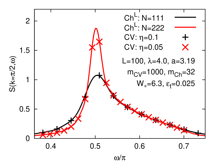
Fig. 4: (Color online) Comparison of CheMPS vs. correction vector (CV) calculations of $S(k=\pi/2,\omega)$ for a Heisenberg chain: Lines show Chebyshev results reconstructed for $N=118$ and 236 using Lorentz damping, eq:app-cheby-13, with $\lambda=4.0$; symbols show CV results, obtained using broadening parameters of $\eta=0.1$ and 0.05. We expect and indeed find good agreement between lines and symbols, since both Lorentz damping and the correction vector method in effect broaden the spectral function by Lorentzians, whose widths we equated by choosing $a\lambda/N=\eta$ (with $a=3.19$), see Eq. (48), and also fig:kernel-delta. Since $m_{\rm Ch}\ll m_{\rm CV}$, the numerical cost of obtaining an entire curve via Chebychev is dramatically cheaper than calculating a single point via CV, as discussed in the text.

We begin our discussion of CheMPS results by comparing them to those of CV calculations, which are known to be very accurate, though also computationally expensive. The CV method involves a broadening parameter $\eta$ and broadens $\delta$-functions into Lorentzian peaks of width $\eta$. This can be mimicked with CheMPS by using Lorentz damping (with $\lambda=4.0$), since this also produces Lorentzian broadening, representing a $\delta$-function $\delta(\omega^{\prime}-\bar{\omega}^{\prime})$ by a near-Lorentzian peak, albeit with a frequency-dependent width, $\eta^{\prime}_{N,\bar{\omega}^{\prime}}=\sqrt{1-\bar{\omega}^{\prime 2}}\,\lambda/N$ (see Sec. II.1 and fig:kernel-delta). To compare CheMPS results with CV results at given $\eta$, we thus identify $\eta=a\eta^{\prime}_{N,\bar{\omega}^{\prime}}$, where $a$ is the scaling factor from Eqs. (21) and $\bar{\omega}^{\prime}$ is taken to be the rescaled and shifted version of the frequency $\omega_{\rm max}$ at which the peak reaches its maximum. Thus we set the expansion order used for reconstruction to

$$N=\frac{4a}{\eta}{\sqrt{1-(\omega_{\rm max}/a-W^{\prime})^{2}}}\,.$$ (48)

Figure 4 shows such a comparison for the structure factor $S(\pi/2,\omega)$ of a $L=100$ Heisenberg chain. We used two choices of $\eta$ that are large enough to avoid finite-size effects, namely $\eta=0.1$ and 0.05, and set $\omega_{\rm max}=\pi/2$ (cf. $\omega_{1}$ of Eq. (45)). We used MPS dimensions of $m_{\textrm{CV}}=1000$ or $m_{\rm Ch}=32$ for CV or CheMPS calculations, respectively. (Our choice for $m_{\rm CV}$ aimed for achieving highly accurate CV results; for $\eta=0.05$ this required $m_{\rm CV}=1000$, but for $\eta=0.1$, a slightly smaller value for $m_{\rm CV}$ would have sufficed.) We find excellent agreement between the two approaches without adjusting any free parameter, since $N$ is fixed by eq:cv-compare-N. For example, for $\eta=0.05$, $N=255$, the relative error is less than 3 % for all $\omega$.

Since this level of agreement is obtained using $m_{\rm Ch}\ll m_{\rm CV}$, we conclude that CheMPS with Lorentz damping gives results whose accuracy is comparable to those of CV, at dramatically reduced numerical cost. Indeed, for $\eta=0.05$ the calculation of the entire CheMPS spectral function was 25 times faster than that of a single CV data point.

IV.3 Finite-size effects

Let us now analyse the role of finite system size. To this end, it is of course important to understand broadening effects in detail. The fact that CheMPS offers simple and systematic control of broadening via the choice of the expansion order (and damping factors), as will be illustrated below, is very convenient and may regarded as one of its main advantages.

Figure 5(a) shows CheMPS results for the spin structure factors $S(k,\omega)$ of four different momenta $k$, calculated for $L=100$ using Jackson damping. They were reconstructed using the largest expansion order, say $N_{L}$, that does not yet resolve finite-size effects, a choice that will be called optimal broadening. Each curve shows a dominant peak, and we are interested in finding its intrinsic shape $S^{\infty}(k,\omega)$ in the continuum limit of an infinitely long chain ($L\to\infty$). Thus, the following general question arises: under what conditions will a spectrum calculated for finite system size $L$ and reconstructed with finite expansion order $N$, say $S_{N}^{L}(\omega)$, correctly reproduce the desired continuum spectrum $S^{\infty}(\omega)$? The general answer, of course, is that the optimally broadened spectrum should have converged as function of $L$, i.e. the shape of $S_{N_{L}}^{L}(\omega)$ should not change upon increasing $L$. However, for a spectrum with an intrinsic divergence, such as Eq. (46), the peak’s height will never saturate with $L$; at best one can hope to observe $L$-convergence of the shape of its tail, and the proper scaling of its height (Eq. (47)).

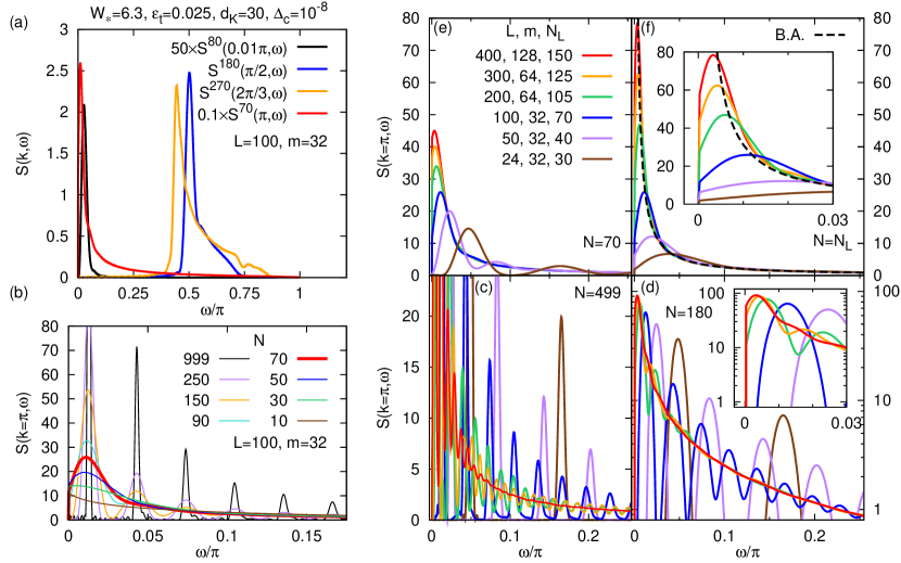
Fig. 5: (Color online) Spin structure factors for a Heisenberg chain, reconstructed using Jackson damping. (a) $S(k,\omega)$ for four choices of momentum $k$, for a chain of length $L=100$. Each spectrum was reconstructed using optimal broadening, i.e. by choosing the largest expansion order, say $N_{L}$ (indicated by superscripts), that does not yet resolve finite-size effects. (b-f) Finite-size analysis of $S(\pi,\omega)$. (b) To determine $N_{L}$ for given $L$ (here 100), several different expansion orders $N$ are considered. Increasing $N$ reduces the effective broadening $\eta_{N}\simeq\mathcal{O}(W_{\!\ast}/N)$ until finite-size subpeaks appear for $N>N_{L}$ (here $N_{L}=70$, bold red curve). (c) Evolution of the finite-size structure with $L$, revealed by fixing $N$ large enough (here = 499) to resolve the first few dominant subpeaks of all curves. There are $L$ dominant subpeaks (not all shown here) within the spectral bandwidth, with average spacing $\omega_{L}\sim 1/L$. (d) Same as (c), but plotted on a semi-log scale, and with somewhat smaller $N$ (here = 180), chosen to be somewhat larger than the optimal broadening $N_{L}$ for the largest $L$ (here $N_{300}=125$). As $L$ increases and $\omega_{L}$ decreases, the subpeaks coalesce toward the intrinsic lineshape $S^{\infty}(k,\omega)$. (e) When $L$ is increased at fixed $N$ (here 70), finite-size effects disappear once $\omega_{L}$ drops below the effective broadening $\eta_{N}$, resulting in a smooth spectral function. (f) In contrast, when $L$ is increased while using optimal broadening, $N=N_{L}$ (i.e. $\eta_{N}$ just above $\omega_{L}$), none of the curves show finite-size effects, and the resulting main peak is sharper than in (e). In both (e) and (f), the peak height shows no indications of converging with $L$, reflecting the fact that the true peak shape involves an $\omega^{-1}[\ln\omega]^{-1/2}$ divergence. Moreover, the CheMPS curves in (f) show signs of overbroadening when compared to the exact Bethe Ansatz result (dashed), from Ref. Caux2006, .

To illustrate the nature of finite-size effects and the role of $N$ in revealing or hiding them, fig:finite-size-analysis(b) shows $S(\pi,\omega)$ for $L=100$ and several values of $N$, both smaller and larger than $N_{L}$. As $N$ is increased and the effective broadening $\eta_{N}\simeq\mathcal{O}(W_{\ast}/N)$ decreases, the main peak of the initially very broad and smooth spectral function becomes sharper. Optimal broadening in fig:finite-size-analysis(b) corresponds to $N_{L}\simeq 70$, beyond which additional “wiggles” emerge. These develop, with beautifully uniform resolution, into dominant subpeaks as $N$ is increased further. The discrete subpeaks reflect the quantized energies of spin-wave excitations in a finite system. With sufficiently high resolution ($N=999$ in fig:finite-size-analysis(b)) numerous additional minor subpeaks emerge, but their weight is very small compared to that of the dominant subpeaks. This fact is important, since it implies that the structure factor of a finite-size system is exhausted almost fully by the set of dominant subpeaks, with very small intrinsic widths.

We have checked that there are $\mathcal{O}(L)$ dominant subpeaks within the spectral bandwidth of $S(k,\omega)$. Correspondingly, the average spacing between dominant subpeaks, to be called the finite-size energy scale $\omega_{L}$, is proportional to $\frac{1}{L}$ (fig:finite-size-analysis(c,d)). The weight of each subpeak decreases similarly, ensuring that the total weight in a given frequency interval converges as $L\to\infty$. The inverse subpeak spacing $\hbar/\omega_{L}$ corresponds to the Heisenberg time, i.e. the time within which a spin wave packet propagates the length of the system.

Figures 5(e,f) illustrate two slightly different broadening strategies. In fig:finite-size-analysis(e), $L$ is increased for fixed $N$: the distinct subpeaks increasingly overlap, resulting in a smooth spectral function once $\omega_{L}$ drops below $\eta_{N}$. In fig:finite-size-analysis(f) optimal broadening is used ($\eta_{N}$ just larger than $\omega_{L}$: now no subpeaks are visible, and the $L$-evolution of the main peak is revealed with better resolution.

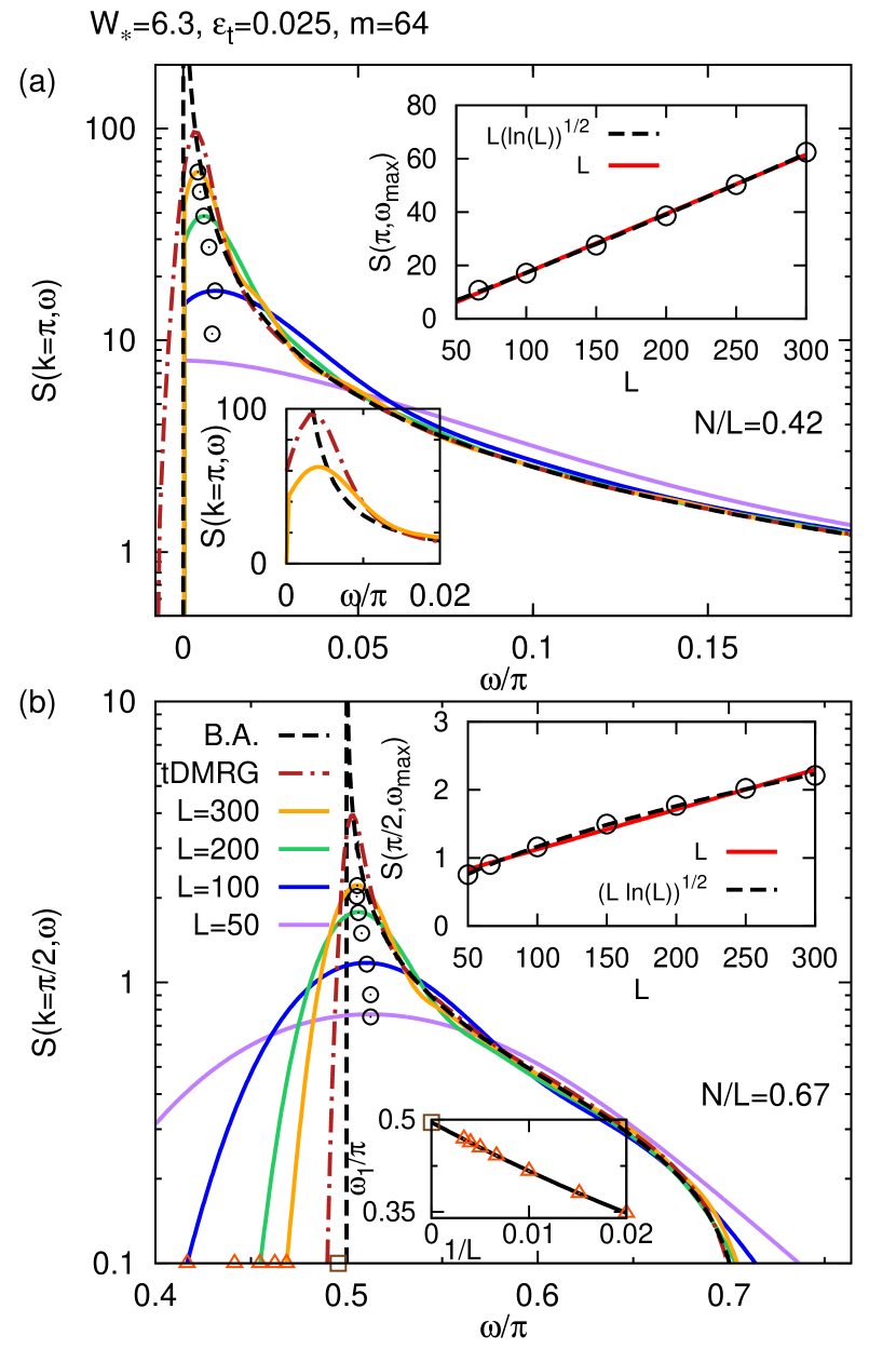
Fig. 6: (Color online) Comparison of CheMPS, Bethe Ansatz and tDMRG + prediction, for HAFM structure factors with (a) $k=\pi$ and (b) $k=\pi/2$. Dashed lines: Bethe Ansatz results for $L=\infty$, from Ref. Caux2006, . Dashed-dotted lines: tDMRG results, from Ref. BarthelSchollwoeckWhite2009, . Other lines show CheMPS results for $L=50,100,200,300$, reconstructed using a fixed ratio of $N/L$, namely 0.42 for (a) and 0.67 for (b). Circles mark Chebyshev peak maxima, also for $L=66,150$ and 250, for which no curves are shown. The lower inset in (a) zooms into the peak region using a linear scale, illustrating overbroadening. The upper insets of (a,b) show the peak heights vs. $L$ (circles), together with a fit to the Bethe-Ansatz expectation from Eq. (46) (dashed line) or to a straight line (solid line). In (b), triangles mark the lower threshold frequencies for which $S(\pi/2,\omega)$ equals a fixed, small value, arbitrarily chosen as 0.1. Their $1/L\to 0$ extrapolation, shown in lower inset, gives an estimate for the lower threshold frequency, namely $\omega_{1}/\pi=0.496$ (marked by a square); the exact value is $1/2$.

In both Figs. 5(e) and 5(f), the peak height shows no indications of converging with increasing $L$. (The same is true for the data of fig:finite-size-analysis(a).) This reflects the intrinsic divergence of the peak height expected from Eq. (46). Figures 6(a) and 6(b) contain a quantitative analysis of this divergence, for $S(\pi,\omega)$ and $S(\pi/2,\omega)$, respectively. The shape of the divergencies for an infinite system are shown by the thick solid lines, representing exact Bethe Ansatz results from Ref. Caux2006, . Thin dashed lines show results from tDMRG from Ref. BarthelSchollwoeckWhite2009, for $L=100$, and thin solid lines CheMPS results for several system sizes between $L=50$ and 300. For CheMPS spectral reconstruction, we determined the expansion order $N_{300}$ that ensures optimal broadening for $L=300$, and used a fixed ratio of $N/L=N_{300}/300$ for all curves (namely 0.42 or 0.67 for Figs. 4(a,b), respectively). CheMPS (for $L=300$) and tDMRG reproduce the peak’s tail and flank well, but clearly and expectedly are unable to produce a true divergence at the lower threshold frequency. Nevertheless, the insets show that the manner in which the CheMPS peak heights increase with $L$ is indeed consistent with Eq. (46). (For the limited range of available system sizes, however, a reliable distinction between $L[\ln(L)]^{1/2}$, $[L\ln(L)]^{1/2}$ or $L$ behavior is not possible.)

It is also possible to determine the lower threshold frequency $\omega_{1}$ rather accurately from the CheMPS results by doing an $1/L$ extrapolation. We illustrate this in fig:spin-L-compare(b) by extrapolating the frequencies at which $S(\pi/2,\omega)=0.1$ (triangles). Since the data exhibit a slight curvature when plotted against $1/L$ (see lower inset of fig:spin-L-compare(b)), they were fitted using a second order polynomial in $1/L$. Extrapolating the fit to $1/L=0$ yields $\omega_{1}=0.496\pi$ (marked by a square), in good agreement with the prediction $\omega_{1}=\pi/2$ from Eq. (45).

IV.4 Discrete representation of spectral function

In both fig:finite-size-analysis(f) and fig:spin-L-compare, the right flank of the peak still bears signatures of overbroadening: the curve for a given $L$ lies above those for larger $L$ (before bending over towards its peak), and all curves lie significantly above the exact Bethe Ansatz curve (dashed line). One way of reducing this broadening would be to simply increase $L$, but this is numerically costly. Clearly, alternative strategies for reducing finite-size effects would be desirable. One such scheme, involving linear prediction in the time domain, will be discussed in the next subsection. Here we present another, which exploits the ability of CheMPS to accurately resolve finite-size peaks.

The origin of overbroadening is clear: when neighboring subpeaks are broadened enough to overlap, weight is inevitably transfered from large peaks to smaller peaks. This effect is negligible only in the limit $L\to\infty$, where the subpeak spacing becomes negligible. To avoid overbroadening for a finite-$L$ system, one thus has to analyse spectra for which $N$ is large enough that subpeaks do not overlap significantly, such as that shown in fig:finite-size-analysis(b).

To be concrete, let us represent the true, discrete spectrum of a system of size $L$ by a sum of peaks, enumerated by a counting index $\alpha$, with position $\Omega_{\alpha}$, width $\bar{\eta}_{\alpha}$, weight $W_{\alpha}$ and Gaussian shape $K^{J}$ (cf. Eq. (18a)):

$$S^{L}(k,\omega)\simeq\sum_{\alpha}W_{\alpha}K^{J}_{\bar{\eta}_{\alpha}}(\omega-\Omega_{\alpha})\;.$$ (49)

Its Chebyshev reconstruction with Jackson damping, say $S_{N}^{L}(k,\omega)$, will have the same form, except that the peaks will be broadened to have widths, $\eta_{\alpha}=(\bar{\eta}_{\alpha}^{2}+\eta_{N,\alpha}^{2})^{1/2}$, as explained before Eq. (19). If $N$ is large enough, the broadened peaks will still be clearly separated (as for $N=999$ or 250 in fig:finite-size-analysis). By fitting each peak (separately, one by one) to a Gaussian, one can determine its position $\Omega_{\alpha}$, weight $W_{\alpha}$ and effective width $\eta_{\alpha}$, and deduce the intrinsic width via $\bar{\eta}_{\alpha}=(\eta_{\alpha}^{2}-\eta_{N,\alpha}^{2})^{1/2}$. We find (not shown) that the intrinsic width grows with increasing frequency $\Omega_{\alpha}$. This implies, not unexpectedly, that higher-lying spin-wave excitations have shorter life-times. However, it also implies that higher-lying peaks eventually start to overlap, so that the analysis to be described below is feasible only for a limited number of low-lying peaks.

The discrete peaks suggest a natural partitioning of the frequency spectrum into intervals $I_{\alpha}$: each contains one peak of weight $W_{\alpha}$ at position $\Omega_{\alpha}$, extends halfway to the next peaks at $\Omega_{\alpha\pm 1}$ on either side, and has width $\Delta_{\alpha}=(\Omega_{\alpha+1}-\Omega_{\alpha-1})/2$. The first interval above the lower spectral threshold ($\omega_{1}$) is defined slightly differently: $I_{1}$ has lower bound $\omega_{1}$ and width $\Delta_{1}=(\Omega_{1}+\Omega_{2})/2-\omega_{1}$.

Now, to produce a smooth curve devoid of finite-size effects, the subpeaks must be broadened until they overlap substantially. However, if the weights in two neighboring intervals differ, say $W_{\alpha}>W_{\alpha+1}$, such broadening inevitably transfers weight from interval $I_{\alpha}$ to $I_{\alpha+1}$, resulting in overbroadening.

Such overbroadening can be avoided by constructing a discrete representation of the spectral function, $S_{\rm dis}(k,\Omega_{\alpha})$, defined by the set of coordinates

$$\{(\Omega_{\alpha},S_{\alpha})\},\quad\textrm{with}\quad S_{\alpha}=S_{\rm dis}(k,\Omega_{\alpha})=W_{\alpha}/\Delta_{\alpha}\;.\quad\phantom{.}$$ (50)

The identification of $S_{\alpha}$ with $W_{\alpha}/\Delta_{\alpha}$ follows from applying the definition of a spectral function, namely spectral weight per unit frequency interval, to the interval $I_{\alpha}$.

Figure 7 shows the resulting discrete data points for four different system sizes. Remarkably, they all fall onto the same curve, which agrees well with the Bethe Ansatz result (dashed line). In particular, the first two or three data points for each $L$ lie right on top of the Bethe Ansatz curve (dashed), see fig:discrete-spectrum, left inset, beautifully mapping out the true shape of the spectral function down to the lowest discrete excitation frequency $\Omega_{\alpha}$ that exists for that $L$. Evidently, the discrete spectral function is completely free from broadening artifacts, in marked contrast to the optimally broadened curves shown for $L=200$ and 400 (solid lines) (compare also fig:finite-size-analysis(f)). This advantage comes at the price of specifying the spectral function only at discrete points, not via a continuous curve. However, for a system of finite size, such discreteness is fundamentally unavoidable. The good news is that the continuum curve $S^{\infty}_{N}(k,\omega)$ is evidently well mimicked by the discrete representation $\{(\Omega_{\alpha},S_{\alpha})\}$, and that CheMPS allows the latter to be determined in a straightforward fashion for system sizes well beyond what can be done with exact diagonalization. We are not aware of any other numerical many-body method capable of doing so for system sizes as large as those considered here.

For larger frequencies the scatter of the discrete data w.r.t. the Bethe Ansatz curve increases, reflecting the fact that subpeaks begin to overlap there, making the extraction of discrete data increasingly difficult. However, this is not a serious concern, since in this frequency regime optimal broadening is able to produce smooth spectra in good agreement with Bethe Ansatz anyway.

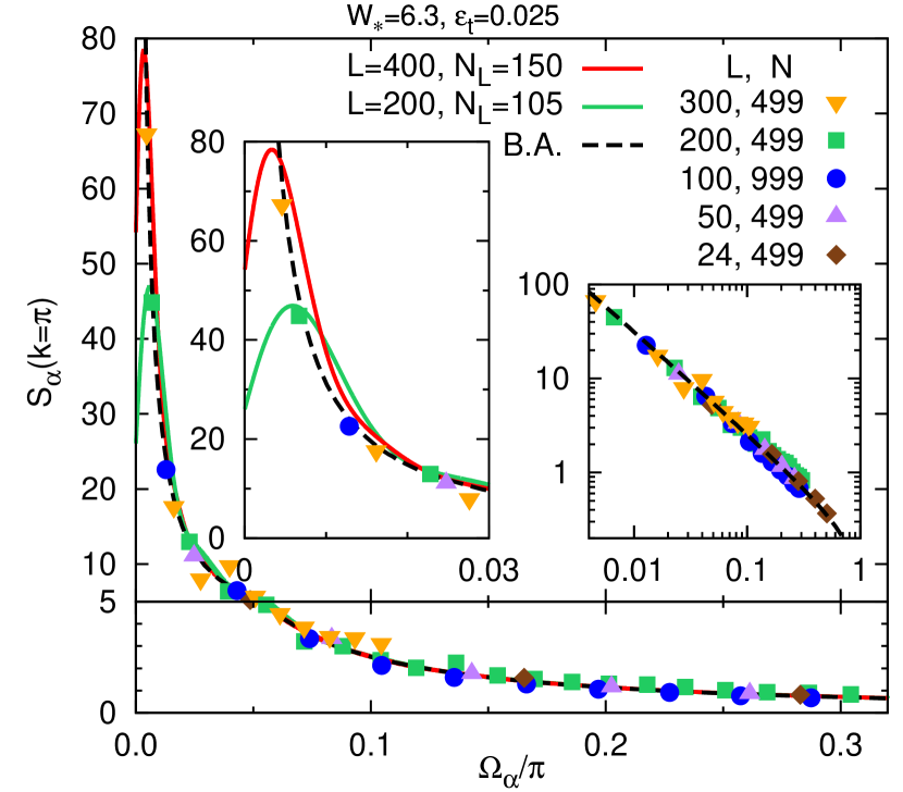
Fig. 7: (Color online) Discrete representation (Eq. (50)) of the structure factor $S_{\alpha}=S_{\rm dis}(\pi,\Omega_{\alpha})$ (symbols), for five different system sizes. (The lower panel uses an enlarged vertical scale, to zoom in on the tail region.) For comparison, the Bethe Ansatz result (dashed line) and two optimally broadened spectra, for $L=400$ and 200 (solid lines), are also shown. Left inset: zoom to low frequencies, showing that the discrete data completely avoids overbroadening, in contrast to the optimally broadened spectra. Right inset: log-log version of main plot. The frequency range does not extend low enough to be able to uncover the pure asymptotic predicted by Eq. (46b).

To conclude this subsection, let us summarize the two main results of our finite-size analysis. The first concerns physics: for a chain of finite chain of $L$ sites, the structure factor is dominated by a set of $\mathcal{O}(L)$ sharp subpeaks, whose spacing and weight scale as $1/L$. The second concerns methodology: CheMPS very conveniently allows this structure to be revealed or hidden, by simply choosing $N$ appropriately. Moreover, it can exploit information on the positions and weights of the discrete subpeaks to largely eliminate broadening artefacts.

IV.5 Comparison of tCheMPS to tDMRG

Another possible scheme for reducing finite-size effects is to work in the time domain using linear prediction, as shown in Ref. BarthelSchollwoeckWhite2009, for the HAFM. The idea is to calculate the Fourier transform of $S(k,\omega)$, namely

$$S(k,t)=\sum_{x=1}^{L}e^{ik(x-x^{\prime})}\langle{\hat{{\boldsymbol{S}}}_{x}(t)\hat{{\boldsymbol{S}}}_{x^{\prime}}(0)}\rangle\,,$$ (51)

with $x^{\prime}$ chosen near the middle of the chain, and $t$ chosen small enough that the spin excitation created at $x^{\prime}$ does not reach the edge of the system within $t$. The function $S(k,t)$ thus obtained will contain only weak finite-size effects. It is then extrapolated to larger times via linear prediction techniques, PressTeukolskyVetterlingFlannery2007 ; PereiraWhiteAffleck2008 ; WhiteAffleck2008 ; BarthelSchollwoeckWhite2009 exploiting the fact that momentum excitations typically exhibit damped harmonic dynamics, whose time-dependence can be extrapolated quite accurately. Since the extrapolated function extends to very large times, its Fourier transform yields good spectral resolution at low frequenciesPressTeukolskyVetterlingFlannery2007 (with an accuracy that depends on that achieved during linear prediction).

In Ref. BarthelSchollwoeckWhite2009, the input correlator needed for linear prediction, $S(k,t)$, was calculated using tDMRG. (Two examples of the resulting spectra are included in our Fig. 6.) We note that $S(k,t)$ can also be calculated using CheMPS in the time-domain, to be called tCheMPS. Indeed the numerical cost for calculating $S(k,t)$ by evaluating the requisite correlators $\langle{\hat{{\boldsymbol{S}}}_{x}(t)\hat{{\boldsymbol{S}}}_{x^{\prime}}(0)}\rangle$ via Eq. (28) is essentially the same as calculating its Fourier transform $S(k,\omega)$ via Eq. (23), since the corresponding Chebyshev moments $\mu_{n}$ can be calculated using the same recursion scheme. In fact, if one defines $\hat{{\boldsymbol{S}}}_{k}$ in Eq. (43) using a pure exponential $e^{ikj}$ instead of a sin function, the Chebyshev moments needed for $S(k,t)$ are simply linear combinations of those of $S(k,\omega)$.

To gauge the accuracy of tCheMPS, we have calculated $S(\pi/2,t)$ using both tCheMPS and tDMRG. Figure 8(a) compares the results, and fig:time-skt(b) characterizes the differences. We view the tDMRG results as benchmark, because for the times of interest, we have checked them to be well converged (with errors $\lesssim 10^{-3}$ for $t<50$, see fig:time-skt(b), dashed-dotted line). As expected, the agreement between tCheMPS and tDMRG is better for larger $m$. The differences are very small, but grow with time, from being (for $m=64$) below $10^{-3}$ for $t\lesssim 10$ to around $10^{-2}$ for $t\simeq 30$, beyond which finite-size effects start to appear.

More generally, the results of fig:time-skt illustrate that CheMPS offers a viable route to time evolution for situations where extreme accuracy is not required. Further comments on this prospect are included in the outlook, Sec. VII.

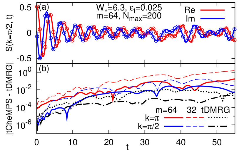
Fig. 8: (Color online) (a) Time dependence of $S(\pi/2,t)$, calculated with tCheMPS (lines) and tDMRG (symbols). Solid and dashed lines show, respectively, the real and imaginary parts of $S$. (b) The differences between tCheMPS and tDMRG (with a specified truncation error of $10^{-6}$) of $S(k,t)$ for two values of $k$, and two values of $m$ (dashed/solid). To estimate the accuracy of tDMRG, we also show (dashed-dotted) the differences between two tDMRG calculations performed with different truncation error thresholds, namely $10^{-5}$ and $10^{-6}$, requiring up to $m=75$ or 125 states, respectively.

V Error analysis

The convergence properties of a Chebyshev expansion are mathematically well controlled and understood (see Eq. (14)), provided that the Chebyshev moments $\mu_{n}$ are known precisely. Their evaluation via CheMPS, however, introduces various sources of numerical errors. This section is devoted to an analysis of these errors. In particular, we seek to determine appropriate choices for the control parameters associated with the various CheMPS tasks listed in Table 1. We perform this analysis mostly for a resonant level model (RLM), describing three local levels coupled to a fermionic bath. This model is introduced and discussed in App. A, which, for the sake of completeness, also includes CheMPS expansions of the corresponding spectral functions. However, the details presented there are not needed for the following discussion.

For the RLM, on the one hand, the CheMPS evaluation of the $\mu_{n}$ is feasible to arbitrarily high orders, and on the other, exact diagonalization (to be denoted by sub- or superscript ED) of the single-particle Hamiltonian allows both the spectral function and the Chebyshev moments $\mu_{n}$ to be found exactly. We use the RLM-parameters specified in App. A throughout and focus mainly on the properties of one of its correlators, $\mathcal{A}^{-}_{11}$ (without displaying corresponding sub- and superscripts), which is defined in Eq. (62) and whose behavior is representative for that of $\mathcal{A}^{\pm}_{ij}$.

V.1 Definition of error measures

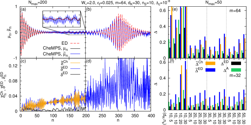
Fig. 9: Comparison of CheMPS and ED results for Chebyshev moments of the RLM spectral function $A_{11}^{-}$. (a,b) show $\mu_{n}$- and $\tilde{\mu}_{n}$ moments (Eqs. (25), (34)) and (c,d) the $n$-dependent error measures $\delta^{\rm ED}_{n}$, $\tilde{\delta}^{\rm ED}_{n}$ and $\tilde{\delta}^{\rm Ch}_{n}$ (Eqs. 52), plotted in (a,c) for $n<N_{\rm max}=200$ and in (b,d) for $N_{\rm max}\leq n<2N_{\rm max}$. In (b), the increase in moment magnitude starting around $n\simeq 250$ marks the onset of resolving finite-size structure in the spectral function. (e,f) show the cumulative error measures $\Delta^{{\rm ED}}$, $\tilde{\Delta}^{{\rm ED}}$, $\tilde{\Delta}^{\rm Ch}$ (Eqs. (53)) and $\Delta^{A}$ (Eq. (54)) for various combinations of the MPS dimension $m$, the number of energy truncation sweeps $n_{S}$ and the Krylov subspace dimension $d_{K}$.

We will analyse both $\mu_{n}$- and $\tilde{\mu}_{n}$-moments, calculated from Eqs. (25) and (34), respectively. The differences between CheMPS and ED can be quantified by the error measures

$$\delta^{\rm ED}_{n} = \left|\mu_{n}^{\rm CheMPS}-\mu_{n}^{\rm ED}\right|\,,\quad n<N_{\rm max}\,,$$ (52a)

$$\tilde{\delta}^{\rm ED}_{n} = \left|\tilde{\mu}_{n}^{\rm CheMPS}-\mu_{n}^{\rm ED}\right|\,,\quad n<2N_{\rm max}\,.$$ (52b)

Moreover, to characterize the accuracy of CheMPS moments without referring to exact results, we also consider

$$\tilde{\delta}^{\rm Ch}_{n} = \left|\tilde{\mu}_{n}^{\rm CheMPS}-\mu_{n}^{\rm CheMPS}\right|\,,\quad n<N_{\rm max}\,.$$ (52c)

We will also use cumulative versions of these, namely

$$\Delta^{{\rm ED}} =\sqrt{\sum_{n=0}^{N_{\rm max}-1}\left(\delta_{n}^{\rm ED}\right)^{2}}\;,$$ (53a)

$$\tilde{\Delta}^{\rm ED} =\sqrt{{\Delta^{{\rm ED}}}^{2}+\sum_{n=N_{\rm max}}^{2N_{\rm max}-1}(\tilde{\delta}_{n}^{\rm ED})^{2}}\;,$$ (53b)

$$\tilde{\Delta}^{\rm Ch} =\sqrt{\sum_{n=0}^{N_{\rm max}-1}(\tilde{\delta}_{n}^{{\rm Ch}})^{2}}\;.$$ (53c)

Furthermore, we also introduce an integrated error measure for undamped spectral functions (using Jackson damping would yield qualitatively similar error measures):

$$\Delta^{\rm A}=\sqrt{\int_{0}^{W_{\!\ast}}d\omega\left|\mathcal{A}^{2N_{\rm max}}(\pm\omega)-\mathcal{A}^{\infty}(\pm\omega)\right|^{2}}\,.$$ (54)

Here we use $\pm$ for $\mathcal{A^{\pm}}(\omega)$ spectra proportional to $\theta(\pm\omega)$ (see Eq. (62)), and employ $\mu_{n}$-moments for $n<N_{\rm max}$ and $\tilde{\mu}_{n}$-moments for $N_{\rm max}\leq n<2N_{\rm max}$ during spectral reconstruction. (Note that $\tilde{\Delta}^{\rm ED}$ of Eq. (53b) was constructed to reflect this combination of $\mu_{n}$ and $\tilde{\mu}_{n}$.)

V.2 Comparison of CheMPS and ED moments

Figure 9 contains the results of our comparison of CheMPS and ED moments for a fixed set of CheMPS parameters, stated in the figure legend. Figures 9(a,b) show Chebyshev moments $\mu_{n}$ and $\tilde{\mu}_{n}$, Figs. 9(c,d) the $n$-dependent error measures, $\delta^{\rm ED}_{n}$, $\tilde{\delta}^{\rm ED}_{n}$ and $\tilde{\delta}^{\rm Ch}_{n}$. From Fig. 9(c) we note several points: (i) For $n\leq N_{\rm max}$, the $\mu_{n}$-moments from CheMPS and ED agree to within about 1%; this illustrates that CheMPS is able to generate rather accurate results for several hundered moments at modest computational costs. (ii) $\mu_{n}$-moments are more accurate than $\tilde{\mu}_{n}$-moments; the reason is that each $\mu_{n}$-moment depends on only one Chebyshev vector, whereas each $\tilde{\mu}_{n}$-moment depends on two. (Note, though, that if spectral reconstruction is performed by employing both $\mu_{n}$-moments for $n\leq N_{\rm max}$ and $\tilde{\mu}_{n}$-moments for $n>N_{\rm max}$ (as done, e.g., for Figs. 5 and 13), the reduced accuracy of the $\tilde{\mu}_{n}$-moments is offset to some extent if damping factors $g_{n}$ are employed, since these decay to 0 as $n$ approaches $N$, see inset of fig:kernel-delta.) (iii) The error measures $\tilde{\delta}^{\rm Ch}_{n}$ and $\tilde{\delta}^{\rm ED}_{n}$ are of comparable magnitude; this implies that $\tilde{\delta}^{\rm Ch}_{n}$ is a useful error quantifyer if exact results are not available.

The way in which theses errors depend on the various CheMPS control parameters can conveniently be analysed using the cumulative error measures $\Delta^{{\rm ED}}$, $\tilde{\Delta}^{{\rm ED}}$, $\tilde{\Delta}^{\rm Ch}$ and $\Delta^{A}$. These are shown in Figs. 9(e,f) for various combinations of $m$, $n_{S}$ and $d_{K}$. Several observations can be made: (iv) When increasing the Krylov subspace dimension $d_{K}$, all cumulative errors decrease from $d_{K}=20$ to 30, but the decrease saturates beyond $d_{K}=30$. (v) Increasing the number of energy truncation sweeps beyond $n_{S}=10$ does not necessarily reduce the cumulative errors; on the contrary, most actually increase, implying that energy truncation sweeping should not be overdone. (iv) The cumulative errors depend only weakly on the MPS dimension $m$ (except for $d_{K}=10$, which is unreliable anyway), and tend to be smaller(!) for $m=32$ than 64 (compare Figs. 9(e) and 9(f)). This trend suggest that the errors introduced by energy truncation grow if the mismatch between $m$ and $d_{K}$ grows. Points (iv) to (vi) indicate that energy truncation is the limiting factor for reducing CheMPS errors, a fact that will be elaborated on in Sec. V.3 below.

To identify an optimal combination of CheMPS control parameters, we have collected error data such as those shown in Figs. 9(e,f) for each possible combination of $W_{\!\ast}=(1.1,1.5,2.0)$, $\epsilon_{\rm t}=(0.1,0.01,0.025)$, $d_{K}=(10,20,30,50)$, $n_{S}=(5,10,20)$, and several $m$-values, for fixed maximum recursion number $N_{\rm max}=50$ and convergence threshold $\Delta_{\rm c}=10^{-8}$. We concluded that the choices $d_{K}=30$, $n_{S}=10$, $W_{\!\ast}=2{W_{\!\!\mathcal{A}}}$ and $\epsilon_{\rm t}=0.025$ robustly yield good results (also for the HAFM), and hence list these as recommended values in Table 1. Actually, the precise choice of $\epsilon_{\rm t}$ has only small effects on the error, as long as $W_{\!\ast}$ is chosen big enough. If $W_{\!\ast}$ is too small, however, the resulting spectral function will loose some weight at high frequencies, because numerical errors may cause energy truncation to effectively also project out some contributions with energies smaller than the energy truncation threshold $\varepsilon_{P}$.

V.3 Errors induced by recursion fitting and energy truncation

To better understand the error dependence on $m$, $d_{K}$ and $n_{S}$ observed in points (iv) to (vi) of Sec. V.2 above, let us analyse in more detail the errors generatured during recurrence fitting (Sec. III.1) and energy truncation (Sec. III.2). The error incurred when constructing $|t_{n}\rangle$ from $|t_{n-1}\rangle$ and $|t_{n-2}\rangle$ using recurrence fitting is characterized by the relative fitting error $\Delta^{\rm r}_{\rm fit}={\Delta_{\rm fit}}/{\mathinner{\lVert|{t_{n}}\rangle\rVert}}$ (Eq. (31)). The effect of projecting out high-energy states using energy truncation, $|{t_{n}}\rangle\mapsto P_{\rm tr}|{t_{n}}\rangle$, can be characterized by the average truncated weight per site during one truncation sweep, $N_{{\rm tr}}^{{\rm sweep}}$ (Eq. (40)), and by the relative truncation-induced state change $\Delta^{\rm r}_{{\rm tr}}={\Delta_{{\rm tr}}}/{\mathinner{\lVert|{t_{n}}\rangle\rVert}}$ (Eq. (41)). The latter measures intended changes in the state due to the truncation of high energy weight, but also incorporates the effects of unavoidable numerical errors.

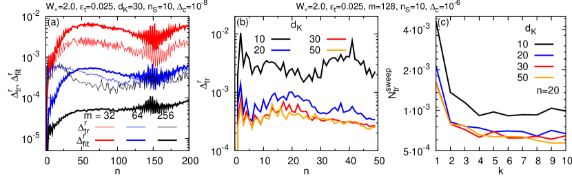
Fig. 10: (Color online) (a) Relative fitting error $\Delta^{\rm r}_{\rm fit}=\Delta_{\rm fit}/\mathinner{\lVert|{t_{n}}\rangle\rVert}$ (Eq. (31)) and relative truncation-induced state change $\Delta^{\rm r}_{{\rm tr}}=\Delta_{{\rm tr}}/\mathinner{\lVert|{t_{n}}\rangle\rVert}$ (Eq. (41)), as functions of recursion number $n$, for three different choices of MPS dimension $m$. Both quantities decrease with increasing $m$, but $\Delta^{\rm r}_{\rm fit}$ more strongly so since recurrence fitting is a strictly variational procedure, whereas energy truncation is not. (b) $\Delta^{\rm r}_{{\rm tr}}$ as function of $n$, and (c) the average truncated weight per site $N_{{\rm tr}}^{\rm sweep}$ (for $n=20$) as function of truncation sweep number $k$. Both (b) and (c) show results for four choices of Krylov subspace dimension $d_{K}$, whose $d_{K}$-dependence saturates beyond $d_{K}=30$.

These quantities are analysed in fig:fidelity-compare in dependence on $m$, $d_{K}$ and $n_{S}$. Continuing our list of observations from the previous subsection, we note the following features: (vii) Both $\Delta^{\rm r}_{\rm fit}$ and $\Delta^{\rm r}_{{\rm tr}}$ are smaller than 1% already for $m=32$ (fig:fidelity-compare(a)), in accord with similar error margins for $\delta^{\rm ED}_{n}$ in fig:rlm-coeffs-illustrate(c). (viii) Both $\Delta^{\rm r}_{\rm fit}$ and $\Delta^{\rm r}_{{\rm tr}}$ decrease with increasing $m$, but $\Delta^{\rm r}_{{\rm tr}}$ does so more slowly, and its decrease seems to saturate beyond $m=64$. This implies that energy truncation is the main limiting factor for CheMPS. The reason is that the intended purpose of energy truncation, namely to strip $|t_{n}\rangle$ from its high-energy components, modifies it in a way whose errors cannot be reduced to arbitrarily small values. Indeed, this is illustrated by the following two points: (ix) While both $\Delta_{{\rm tr}}$ and $N_{{\rm tr}}^{\rm sweep}$ initially decrease with increasing Krylov subspace dimension $d_{K}$, the decrease saturates for $d_{K}\gtrsim 30$ (fig:fidelity-compare(b,c)); (x) While $N_{{\rm tr}}^{\rm sweep}$ initially decreases with the number of sweeps $n_{S}$, the decrease saturates already for $n_{S}\lesssim 10$ fig:fidelity-compare(c). Qualitatively, the behavior shown in fig:fidelity-compare(c) is robust. (However, the choices of other CheMPS control parameters do influence its quantitative details, such as the $d_{K}$ beyond which $N_{{\rm tr}}^{\rm sweep}$ becomes $d_{K}$-independent.) The lack of saturation of $N_{{\rm tr}}^{\rm sweep}$ with $n_{S}$ implies that there is no automatic stopping criterion for truncation sweeps. Instead, the choice of $n_{S}$ can be optimized as described in Sec. V.2, where we already concluded that taking $n_{S}$ much larger than 10 actually deteriorates the results.

Of course, truncation-induced errors can be avoided by simply using the full bandwidth, $W_{\!\ast}=W$, for which no trunctation is necessary. However, in our experience the gain in resolution obtained by using, instead, an effective bandwidth $W_{\!\ast}\ll W$, outweighs the small loss in accuracy incurred by the necessity to then perform energy truncation.

VI Density matrix spectra

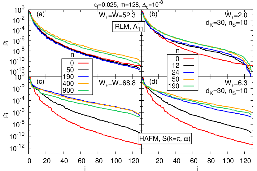
Fig. 11: (Color online) Eigenvalue spectra $\rho_{n}(i)$ of the reduced density matrix at the center of the system for several expansion vectors $|{t_{n}}\rangle$ of (a,b) the RLM with $L_{b}=101$, and (c,d) the HAFM with $L=100$. In (a,c) we used the full many-body bandwidth $W_{\!\ast}=W$ without energy truncation, in (b,d) a reduced effective bandwidth with energy truncation.

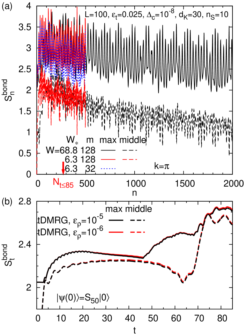
Fig. 12: (Color online) Entanglement or bond entropy $S^{\rm bond}$ for the $k=\pi$ spectral function of the HAFM. (a) $S^{\rm bond}_{n}$ for the Chebyshev vectors $|{t_{n}}\rangle$ and (b) $S^{\rm bond}_{t}$ during the tDMRG time evolution of $e^{-i\hat{H}t}\hat{{\boldsymbol{S}}}_{x=50}|{0}\rangle$. In both (a) and (b), solid and dashed lines show the maximum bond entropy and the bond entropy at the middle of the system, respectively. (a) $S^{\rm bond}_{n}$ is shown for two choices of $W_{\!\ast}$; the dotted line is from a calculation with a reduced $m=32$ and some entropy is lost due to truncation. The red arrow marks the expansion order roughly necessary to reach the time $t=85$ using the tCheMPS technique for $W_{\!\ast}=6.3$, here $N_{t\leq 85}=271$. To reach the same time using $W_{\!\ast}=W=68.8$ an order of expansion of $N_{t\leq 85}=2961$ would be necessary. (b) $S^{\rm bond}_{t}$ is shown for two choices of the truncation error $\epsilon_{\rho}$.

The effects of energy truncation can be understood in more detail by considering the reduced density matrix

$$\hat{\rho}_{n}={\rm Tr}_{\rm half}|t_{n}\rangle\langle t_{n}|$$ (55)

where the trace is over one half of the chain. Let us analyse the $n$-dependence of the spectrum of its eige¡nvalues, say $\rho_{n}(i)$. It can be used to quantify the entanglement encoded in $|t_{n}\rangle$, via the associated entanglement or bond entropy,

$$S_{n}^{\rm bond}=-\sum_{i}\rho_{n}(i)\ln(\rho_{n}(i))\;.$$ (56)

Figure 11 shows such density matrix spectra for both the RLM (panels (a,b)) and the HAFM (panels (c,d)), calculated using both the full many-body bandwidth $W_{\!\ast}=W$ (panels (a,c)) and a smaller effective bandwidth $W_{\!\ast}$ (panels (b,d)). The $n=0$ line in all panels shows the eigenvalue spectrum $\rho_{0}(i)$, which reflects the entanglement encoded in $|{t_{0}}\rangle=\hat{\mathcal{C}}|{0}\rangle$ at the start of the recursion procedure. In principle one would expect the entire spectrum of density matrix eigenvalues $\rho_{n}(i)$ to shift or rise to higher values as $n$ increases, since multiplying $|t_{n-1}\rangle$ by $\hat{H}^{\prime}$ when calculating $|t_{n}\rangle$ (cf. Eq. (30)) generates entanglement entropy. Such a spectral rise with increasing $n$ is indeed observed in all four panels of 11, but the rise eventually saturates for sufficiently large $n$. The speed of the initial stages of the rise differs from panel to panel. For the density matrix spectra calculated without energy truncation (fig:dm-spectrum(a,c)), the initial rise is rather slow, in particular for the RLM (fig:dm-spectrum(a), where the rise is preceded by a slight initial decrease), reflecting the lack of strong correlations of this model. In contrast, for density matrix spectra calculated with energy truncation (fig:dm-spectrum(b,d)), the initial rise is very rapid, and its subsequent saturation sets in at quite small $n$ (of order 20 to 30). Thus, energy truncation evidently has the effect of increasing entanglement entropy. The reason is that the latter is calculated in a different basis (the eigenbasis of $\hat{\rho}_{n}$) than that used to perform energy truncation (the local eigenbasis of $\hat{H}^{\prime}$).

According to fig:dm-spectrum(d), the small MPS dimension of $m=32$ used for the HAFM in fig:finite-size-analysis(a) in effect amounts to discarding the contributions to the reduced density matrix of all states with weight below a threshold of around $10^{-3}$. This threshold is rather large compared to typical DMRG calculations, where characteristic truncation errors lie in the range $10^{-6}$ to $10^{-8}$. It is remarkable that CheMPS is nevertheless able to give rather accurate results (such as reproducing CV results obtained using $m_{\rm CV}=1500$).

This efficiency appears to be an intrinsic feature of CheMPS, arising from the recursive manner in which the Chebyshev vectors $|t_{n}\rangle$ are constructed. Evidence for this conclusion is presented in fig:entropy(a), which shows the bond entropy $S_{n}^{\rm bond}$ associated with $|t_{n}\rangle$ as function of recursion number $n$. Remarkably, the bond entropy shows no tendencies towards unbounded growth, even up to values as large as $n=2000$. Quite to the contrary: although the bond entropy increases somewhat when increasing $m$ from 32 to 128 (with $W_{\!\ast}=6.3$), for either case it tends to decrease with recursion number $n$, and similarly for the choice $W_{\!\ast}=W$ without energy truncation. All of this is very encouraging, since it indicates that $n$ can be increased, apparently at will, without incurring any runaway growth of DMRG truncation errors. The reasons for this fact will be recapitulated in the summary below.

For comparison, fig:entropy(b) shows the bond entropy $S^{\rm bond}_{t}$ of a tDMRG calculation of the time evolution of $|\psi(t)\rangle=e^{-i\hat{H}t}\hat{{\boldsymbol{S}}}_{x=50}|0\rangle$. This entropy is, overall, smaller than the $S^{\rm bond}_{n}$ of the Chebyshev vectors, because the initial state for the time evolution involves an excitation at only one site, whereas the starting state for the CheMPS recursion involved a linear combination of local excitations, $\hat{{\boldsymbol{S}}}_{k}|0\rangle$ (see Eq. (43)). The most striking difference between $S^{\rm bond}_{n}$ and $S^{\rm bond}_{t}$, however, is that the former shows no trend to increase with $n$, whereas the latter does with $t$. The increase in $S^{\rm bond}_{t}$ occurs in spurts, that happen each time a spin wave gets reflected from one of the ends of the system, at which point more numerical resources are required to keep track of the superposition of incident and reflected spin waves. For the present problem, the increase in $S^{\rm bond}_{t}$ was not severe and remained completely under control (staying below $S_{n}^{\rm bond}$ throughout). Nevertheless, we do believe that the contrast between fig:entropy(a) and fig:entropy(b), showing a nonincreasing trend for $S_{n}^{\rm bond}$ vs. an increasing trend for $S_{t}^{\rm bond}$, is striking and significant. It suggests that for situations that feature strong entanglement growth with time, tCheMPS might be a promising alternative to tDMRG.

VII Summary

In this work, we have described CheMPS as a method for calculating zero-temperature spectral functions of one-dimensional quantum lattice models using a combination of a Chebyshev expansion and MPS technology. To summarize our analysis, we would like to highlight what we believe to be the two most important features of CheMPS, namely its efficiency and its control of spectral resolution.

Efficiency. The first main feature is that CheMPS provides an attractive compromise between accuracy and efficiency. It is capable of reproducing correction vector results in the frequency domain and tDMRG results in the time domain with comparably modest numerical resources. In particular, surpringly small values for the MPS dimension of $m$ are sufficient, even for obtaining spectral resolution high enough to resolve finite size effects in great detail. (For example, $m=32$ sufficed for the spin-$\frac{1}{2}$ antiferromagnetic Heisenberg model.) This remarkable efficiency, which we had not anticipated when commencing this study, appears to be a consequence of several factors: (i) CheMPS does not suffer from a runaway growth of DMRG truncation error with increasing $n$, because the information needed to construct the spectral function with a specified accuracy, say $\mathcal{O}(1/N)$, is not encoded in a single state, but uniformly distributed over $N$ distinct Chebyshev vectors $|t_{n}\rangle$. (ii) These can be determined from Chebychev recurrence relations involving only three terms, so that it is never necessary to accurately represent the sum of more than two MPS. (iii) Moreover, these recurrence relations are numerically stable, i.e. the inaccuracies in the calculation of Chebyshev vectors $|t_{n}\rangle$ do not cause the Chebyshev expansion to diverge. (iv) Finally, the accuracy needed for each $|t_{n}\rangle$ is set by that needed for $\mu_{n}=\langle{0}|{\cal B}|{t_{n}}\rangle$ (eq:dmrg-recipe-1), which does not need to be better than the specified accuracy, namely $\mathcal{O}(1/N)$.

For spectral functions with a finite spectral width ${W_{\!\!\mathcal{A}}}$ (which is typically much smaller than the many-body bandwidth $W$), CheMPS offers a further attractive feature for enhancing efficiency: one may use an “effective bandwidth” $W_{\!\ast}$ of order ${W_{\!\!\mathcal{A}}}$ (we typically take $W_{\!\ast}=2{W_{\!\!\mathcal{A}}}$), which enhances spectral resolution by a factor $W/W_{\!\ast}$, at the cost of requiring additional energy trunctation sweeps. The latter are not necessary if one takes $W_{\!\ast}=W$, but then considerably higher expansion orders are necessary to achieve comparable resolution. In our experience the benefits of enhanced resolution offered by the choice $W_{\!\ast}=2{W_{\!\!\mathcal{A}}}$ outweigh the costs of energy truncation.

Control of spectral resolution. The second main feature of CheMPS is that it offers very convenient control of the accuracy and resolution of the resulting spectral function, by simply adjusting the expansion order $N$. This is particularly useful for studying finite-size effects, as exemplified in fig:finite-size-analysis. On the one hand, fig:finite-size-analysis(b) shows very strikingly that the structure factor an HAFM chain of finite length is dominated by a set of discrete subpeaks which may be associated with the quantized eigenenergies of spin wave excitations in a finite system. CheMPS allows the energies and weights of these excitations, and their dependence on $L$, to be determined with unprecedented accuracy and ease, by simply increasing $N$ until the peaks are well resolved. On the other hand, fig:finite-size-analysis(f) shows that the limit $L\to\infty$ may be mimicked by choosing $N$ just small enough that the finite-size subpeaks are smeared out. Though the peak shape thus obtained is slightly overbroadened (see inset of fig:finite-size-analysis(f)), this overbroadening can be eliminated completely (see fig:discrete-spectrum) by using a discrete representation of the spectral function, that uses the energies and weights of the discrete subpeaks as input. The ability to fully eliminate overbroadening effects even for very large many-body systems is, to the best of our knowledge, a unique feature of CheMPS.

On a technical level, the implementation of CheMPS requires only standard MPS techniques, such as the addition of different states and the multiplication of operators. For energy truncation, single-site sweeping needs to be set up with a new kind of local update, as described in sec:dmrg-energy-trunc. However, this procedure is not too different from other known local update prescriptions and can be implemented with modest programming effort.

VIII Outlook

Regarding future applications of CheMPS, two directions for further methodological development appear particularly promising, namely time-dependence and finite temperature. A few comments are due about each.

Time dependence. While the good agreement between tCheMPS and tDMRG reported in fig:time-skt is encouraging, a detailed analysis of tCheMPS should be performed to understand the nature of its error growth with time, and to explore under which conditions, if any, tCheMPS offers competitive advantages relative to tDMRG. On the one hand, tDMRG has the advantage that highly efficient Krylov methods can be used to optimize the evaluation of $e^{-i\hat{H}\Delta t}|\psi(t)\rangle$ w.r.t. the state $|\psi(t)\rangle$ being propagated; however its numerical costs increase rapidly if $|\psi(t)\rangle$ contains a broad spectrum of excited states. On the other hand, CheMPS has the advantage (i) that the Chebychev expansion of the operator $e^{-i\hat{H}t}$ can be applied with equal accuracy to every state in the Hilbert space, in particular also highly excited ones. Moreover, (ii) very large evolution times might be achieved more easily with tCheMPS than tDMRG, since the former represents $|\psi(t)\rangle$ as a sum over many Chebyshev vectors (see Eq. (6)), thereby being potentially less susceptible than tDMRG to the growth of truncation errors (as discussed in the introduction, and exemplified in fig:entropy). We expect that for some applications (i) and/or (ii) may offer advantages for tCheMPS over tDMRG, e.g. for calculating quantum quenches starting from strongly nonequilibrium initial states, but leave a detailed investigation to the future.

Finite temperature. The fact that CheMPS uniformly resolves the entire energy spectrum of $\hat{H}$ suggests that it should be particularly suited for calculating the spectral functions $\mathcal{A}_{T}^{\mathcal{BC}}(\omega)=\int\frac{dt}{2\pi}e^{i\omega t}G_{T}^{\mathcal{BC}}(t)$ of finite temperature correlators such as

$$G_{T}^{\mathcal{BC}}(t)={\rm Tr}[\hat{\rho}_{T}\hat{\mathcal{B}}(t)\hat{\mathcal{C}}(0)]\;,\quad\hat{\rho}_{T}=\frac{e^{-\beta\hat{H}}}{Z}.$$ (57)

According to Ref. Weisse2006, , such a spectral function can be evaluated using Chebyshev expansions by proceeding as follows: Express the partition function as

$$Z=\int d\omega e^{-\beta\omega}\rho(\omega)\;,$$ (58a)

by introducting the density of states

$$\rho(\omega)={\rm Tr}[\delta(\omega-\hat{H})]\;,$$ (58b)

and the spectral function as

$$\mathcal{A}_{T}^{\mathcal{BC}}(\omega) = \frac{1}{Z}\int d\bar{\omega}\,e^{-\beta\bar{\omega}}\mathcal{\rho}^{\mathcal{BC}}(\bar{\omega},\omega+\bar{\omega})\;,$$ (59a)

by introducing the density of matrix elementsWang1994 ; Wang1994a

$$\mathcal{\rho}^{\mathcal{BC}}(\bar{\omega},\omega) = {\rm Tr}[\delta(\bar{\omega}-\hat{H})\,\hat{\mathcal{B}}\,\delta(\omega-\hat{H})\,\hat{\mathcal{C}}]\;.$$ (59b)

Then Chebyshev expand the $\delta$-functions in Eqs. (58b) and (59b) using Eq. (23) (after suitably rescaling Hamiltonian and frequencies). The resulting Chebyshev expansions will contain moments of the form

$$\mu_{n}^{\rho} = {\rm Tr}[T_{n}(\hat{H}^{\prime})]\;,$$ (60a)

$$\mu_{nn^{\prime}}^{\mathcal{BC}} = {\rm Tr}[T_{n}(\hat{H}^{\prime})\,\hat{\mathcal{B}}\,T_{n^{\prime}}(\hat{H}^{\prime})\,\hat{\mathcal{C}}]\;.$$ (60b)

We now note that this framework is very well suited for an MPO implementation, which would consist of three steps: (i) Using Chebyshev recurrence relations, recursively construct and store MPO representations for each operator $T_{n}(\hat{H}^{\prime})$; we expect (based on our experience with the Chebyshev vectors $|t_{n}\rangle$) that this should be possible without runaway costs in numerical resources, since the construction of $T_{n}(\hat{H}^{\prime})$ requires only $\hat{H}^{\prime}T_{n-1}(\hat{H}^{\prime})$ and $T_{n-2}(\hat{H}^{\prime})$. (ii) Calculate the moments in Eqs. (60) by evaluating the traces, which is straightforward in the context of MPS/MPO. (iii) Insert the resulting moments into the reconstructed Chebychev expansions for $\rho(\omega)$ and $\rho^{\mathcal{BC}}(\bar{\omega},\omega)$, and finally evaluate the integrals Eqs. (58a)) and (59a). Note the economy of this scheme: after once constructing the MPO for each $T_{n}(\hat{H}^{\prime})$, and once evaluating the trace for each moment $\mu_{n}^{\rho}$ and $\mu_{nn^{\prime}}^{\mathcal{BC}}$, the spectral function $\mathcal{A}_{T}^{\mathcal{BC}}(\omega)$ can be calculated for arbitrary combinations of $\omega$ and $T$. The implementation of this strategy is left for future studies.

We conclude by remarking that the idea of using Chebyshev expansions in the context of many-body numerics, advocated in inspiring fashion in Ref. Weisse2006, , can be implemented in combination with any method that is able to efficiently apply a Hamiltonian $\hat{H}$ to a state $|\psi\rangle$. Chebyshev expansions optimize the resolution that can be extracted from a limited number of applications of $\hat{H}$. While CheMPS is based on doing this using MPS methods for one-dimensional lattice models, similar developments have been pursued within the context of exact diagonalizationAlvermann2007 ; AlvermannFehske2009 and Monte CarloWeisse2009 methods, and Chebyshev expansions should also be useful in combination with tensor network methods for two-dimensional quantum lattice models.

Appendix A Resonant level model

This appendix introduces the fermionic resonant level model (RLM) that was used for the error analysis of Sec. V, and presents CheMPS results for its spectral functions.

The RLM is defined by the following Hamiltonian:

$$\hat{H}_{\rm RLM} = \sum_{i=1}^{n_{d}}\varepsilon_{i}\hat{d}{}_{i}^{\dagger}\hat{d}{}_{i}^{\phantom{+}}+\sum_{i=1}^{n_{d}}V_{i}\sum_{k=1}^{L_{b}}\left(\hat{d}{}_{i}^{\dagger}\hat{c}{}_{k}^{\phantom{+}}+{\rm h.c.}\right)$$

$$+\sum_{k=1}^{L_{b}}\varepsilon_{k}\hat{c}{}_{k}^{\dagger}\hat{c}{}_{k}^{\phantom{+}}\;.$$

It describes a set of $n_{d}$ discrete, “local”, non-interacting fermion levels with energies $\varepsilon_{i}$, that hybridize with strengths $V_{i}$ with a band of $L_{b}$ $(\gg 1)$ fermion levels with energies $\varepsilon_{k}$, assumed uniformly spaced within the interval $[-W_{b},W_{b}]$. We choose $W_{b}=1$ as unit of energy throughout this section. We will parametrize the hybridization strengths $V_{i}$ in terms of the associated level widths $\Gamma_{i}=\pi\frac{L_{b}}{2}V_{i}^{2}$.

The spectral function $A_{ij}(\omega)\equiv A_{ij}^{+}(\omega)+A_{ij}^{-}(\omega)$ has two contributions,

$$A_{ij}^{+}(\omega)\equiv\mathcal{A}^{d_{i}^{\phantom{*}}d_{j}^{\dagger}}(\omega),\qquad A_{ij}^{-}(\omega)\equiv\mathcal{A}^{d_{j}^{\dagger}d_{i}^{\phantom{+}}}(-\omega)\;,$$ (62)

describing particle and hole excitations, which at $T=0$ are proportional to step functions $\theta(\pm\omega)$ that vanish for $\omega<$ or $>0$, respectively. Since the RLM Hamiltonian is quadratic, the problem can be solved by diagonalizing the single-particle problem. In the continuum limit $L_{b}\rightarrow\infty$, this yields the following exact expression for the spectral function,Hewson1997 for $|\omega|<D_{b}=1$:

$$A^{\infty}_{ij}(\omega) = \lim_{\eta\rightarrow 0^{+}}-\frac{1}{\pi}\Im\left(\left[\omega+i\eta-\Upsilon-\Delta(\omega)\right]^{-1}\right)_{ij},$$ (63)

$$\Upsilon_{ij} = \varepsilon_{i}\delta_{ij},\quad\Delta_{ij}(\omega)=\frac{1}{\pi}\sqrt{\Gamma_{i}\Gamma_{j}}\left(\ln\left|\frac{\omega-D_{b}}{\omega+D_{b}}\right|-i\pi\right)\;,$$

where $\Upsilon$ and $\Delta$ are matrices of dimension $n_{d}\times n_{d}$. The Chebyshev moments $\mu_{n}$ for the finite system of length $L$ can also be found exactly, by evaluating the expectation values Eq. (24) using the (numerically-determined) exact single-particle eigenstates of $\hat{H}$.

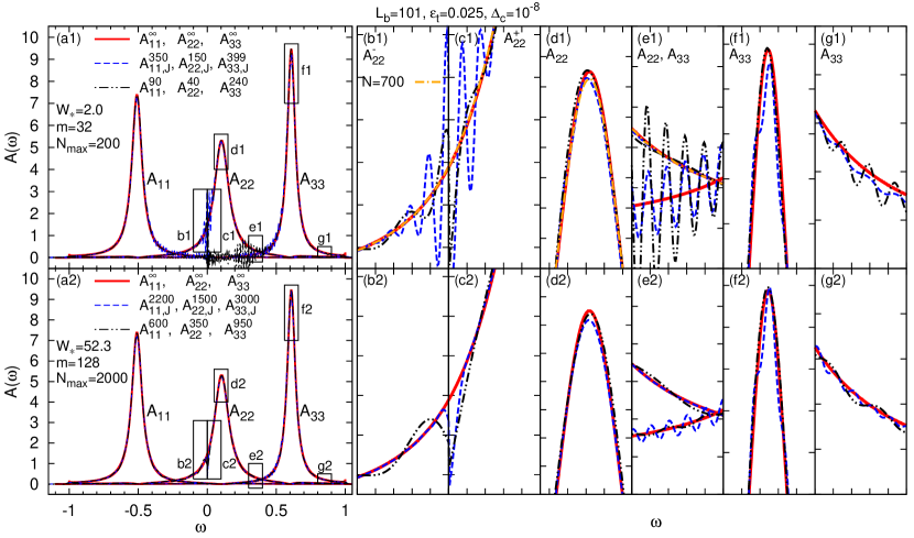
Fig. 13: (Color online) Diagonal spectral functions $\mathcal{A}_{jj}(\omega)$ of a 3-level RLM. Thick solid lines show the continuum limit, $A^{\infty}_{jj}(\omega)$, from eq:rlm-A-cont. Dashed and dashed-double dotted lines show CheMPS results, $\mathcal{A}^{N}_{jj,J}$ or $\mathcal{A}^{N}_{jj}$, with or without Jackson broadening, respectively, calculated for $L_{b}=101$ band levels. For each spectrum, the effective broadening $\eta_{N}$ was taken as large as possible without lowering the peak height significantly below that of $A^{\infty}_{jj}$. In (a1-g1) we used an effective bandwidth of $W_{\!\ast}=2.0$ and in (a2-g2) the full many-body bandwidth $W_{\!\ast}=52.3$. The latter requires significantly larger expansion orders, but exhibits less numerical inaccuracies, compare (b1-g1) and (b2-g2), which represent zooms of the rectangles indicated in (a1) and (a2), respectively. (b,c): Gibbs oscillations arise if $\mathcal{A}^{\pm}(\omega)$ are expanded separately, so that CheMPS attempts to resolve their $\theta(\pm\omega)$ steps. Expanding instead their sum, $\mathcal{A}^{+}(\omega)+\mathcal{A}^{-}(-\omega)$, and performing a Jackson-damped reconstruction, we obtain the smooth dashed-dotted line in (b1-e1) (calculated using ED moments). (d,e) $\mathcal{A}^{N}_{22}$ nicely reproduces $\mathcal{A}^{\infty}_{22}$, because the peak is somewhat broader than $\omega_{L}$. (e-g) $\mathcal{A}^{N}_{33}$ shows small but distinct finite-size wiggles, because the main peak is so sharp and narrow that recovering its height fully, requires an $\eta_{N}$ so small that it is comparable to $\omega_{L}$.

The Hamiltonian (A) corresponds to a “star geometry”, since each local level couples to every band level. For the purposes of using CheMPS, however, it needs to be transformed to a “chain geometry” of the form

$$\begin{split}\hat{H}_{\rm RLM}&=\sum_{i=1}^{n_{d}}\varepsilon_{i}\hat{d}{}_{i}^{\dagger}\hat{d}{}_{i}^{\phantom{+}}+\sum_{i=1}^{n_{d}}\sqrt{\frac{2\Gamma_{i}}{\pi}}\left(\hat{d}{}_{i}^{\dagger}\hat{f}{}_{1}^{\phantom{+}}+{\rm h.c.}\right)\\ &+\sum_{\ell=1}^{L_{b}-1}\lambda_{\ell}\left(\hat{f}{}_{\ell}^{\dagger}\hat{f}{}_{\ell+1}^{\phantom{+}}+{\rm h.c.}\right).\end{split}$$ (64)

This can be achievedBullaCostiPruschke2008 using Lanczos tridiagonalization of the band part of the Hamiltonian, thereby determining the hopping coefficients $\lambda_{\ell}$.

Starting from Eq. (64), we have used CheMPS to calculate the diagonal components $\mathcal{A}_{jj}$ of the RLM spectral function for a model with $n_{d}=3$ local levels. In contrast to Section IV.3, our interest here is not in analysing finite-size effects, but in determining how the CheMPS parameters need to be adjusted to recover the exact continuum function $\mathcal{A}_{jj}^{\infty}$ of Eq. (63). Thus, we purposefully chose a set of model parameters leading to three well-separated peaks of slightly different widths, taking $\varepsilon_{j}\in\{-0.5,0.1,0.6\}$ and $\Gamma_{j}\in\{0.04,0.06,0.03\}$, and chose the number of band levels $L_{b}=101$ large enough that the finite-size spacing $\omega_{L}\simeq 1/L_{b}=0.01$ is somewhat smaller than the smallest peak width, $\Gamma_{3}$. By choosing the expansion order for each curve such that the effective broadening lies in the window between the finite-size spacing and the intrinsic peak width, $\omega_{L}<\eta_{N}<\Gamma_{j}$, it should be possible to reveal the shape of $\mathcal{A}_{jj}^{\infty}$ quite accurately without yet resolving finite-size subpeaks (though traces of the latter might show up for $\mathcal{A}_{33}$, for which this window is small). To this end, we used the following criterion for choosing $N$ when reconstructing $\mathcal{A}^{N}_{jj}$: the effective broadening $\eta_{N}$ was taken as large as possible without lowering the peak height significantly below that of $A^{\infty}_{jj}$ (this corresponds to choosing $\eta_{N}\lesssim\Gamma_{j}$).

The results of these calculations are summarized in Fig. 13; all spectra shown there were obtained by performing separate expansions for the positive and negative branches, $A^{\pm}_{jj}(\omega)$ (with one exception, noted below).

Figures 13(a1-g1) were calculated using an effective bandwidth of $W_{\!\ast}=2.0$ (with $\varepsilon_{t}=0.025$) for each branch, corresponding to roughly twice the spectral width of each branch, which is of order of the single-particle band-width, $W_{A}\simeq W_{b}=1$. For this choice, an MPS dimension of merely $m=32$ was found to suffice for accurate recurrence fitting. Figure 13(a1) illustrates a number of points: (i) By choosing $\eta_{N}$ according to the above criterion of recovering the correct peak height, excellent agreement with the continuum limit $A^{\infty}$ of Eq. (63) is obtained over most of the frequency range. (ii) This is the case both with and without Jackson damping (thin black or blue lines, respectively), but with Jackson damping, higher expansion orders are needed to obtain the correct peak heights, since Jackson damping induces some artificial broadening (by a factor of $\pi$, see Eq. (18a)). (iii) Small oscillations remain in some frequency ranges (see Figs. 13(b1-g1) for zooms). These stem from three sources: finite-size subpeaks, numerical inaccuracies and step function artefacts near $\omega=0$ (cf. points (iv), (vi) and (viii) below, respectively). (iv) For the spectrum with the narrowest peak, $\mathcal{A}_{33}$, the window between $\omega_{L}$ and $\Gamma_{33}$ is so small that the criterion of reproducing the continuum peak height implies that small finite-size subpeak remain visible, see Figs. 13(e1-g1) for zooms. (v) In contrast, such oscillations are almost entirely absent for the broadest peak, $\mathcal{A}_{22}$ (see Figs. 13(d1,e1)), since its width $\Gamma_{2}$ is somewhat larger than $\omega_{L}$.

In order to illustrate the effect of energy truncation, Figs. 13(a2-g2) show the same spectral functions as fig:rmlm-all(a1-g1), but now setting $W_{\!\ast}=W$, the full many-body bandwidth (here = 52.3), so that no energy truncation is needed. This allows us to make some additional instructive observations: (vi) Using the full bandwidth yields results of higher quality, in that numerical artefacts are significantly weaker (except near $\omega=0$), compare Figs. 13(d2-g2) and (d1-g1). The reason is that energy truncation constitutes CheMPS’s dominant source of error (as shown in Section V below); its avoidance thus yields more precise Chebyshev moments $\mu_{n}$, especially for $n>N_{\rm max}$. (vii) However, this improvement is numerically expensive: the increased effective bandwidth neccessitates larger expansion orders $N$, which in turn requires a higher MPS dimension (here $m=128$). (viii) For the present model, it was possible to calculate several thousand moments without encountering numerical instabilities; this illustrates the fact that the Chebychev recurrence relations are numerically stable.

Finally, let us address (ix) the wiggly artefacts near $\omega=0$. They reflect the fact that CheMPS was separately applied to the positive and negative branches of the spectral function, $A^{\pm}(\omega)$, shown in zooms in Figs. 13(b) and fig:rmlm-all(c), respectively. These are proportional to step functions $\theta(\pm\omega)$, and hence abruptly dip to zero for $\omega<0$ or $>0$, respectively. The wiggly artefacts correspond Gibbs oscillations decorating these sharps dips. This problem can be avoided by performing a single Chebyshev expansion of the sum, $\mathcal{A}^{+}(\omega)+\mathcal{A}^{-}(-\omega)$, which is a smooth function and leads to the perfectly smooth long-dashed line in Figs. 13(b,c). This improvement comes at roughly twice the numerical cost, since it requires a doubling of the spectral range to $\omega\in[-W_{A},W_{A}]$: this implies a slight but obvious modification of the transformations from $\omega$ to $\omega^{\prime}$ and from $H$ to $\hat{H}^{\prime}$ to account for the shifted range of $\omega$; and a doubling of $W_{\ast}$ and hence of the expansion order $N$ required to achieve a specified resolution.

The main conclusions from our CheMPS calculations for the RLM are as follows: The strategy of using twice the spectral width as effective bandwidth ($W_{\!\ast}=2W_{A}$) and performing energy truncation (fig:rmlm-all(a)) is a satisfactory compromise between efficiency (only a few hundred Chebyshev moments are needed) and accuracy (for which energy truncation is the main limiting factor). If desired, better results can be obtained by using the full bandwidth ($W_{\!\ast}=W$) and thus avoiding energy truncation, albeit at the cost of significantly increasing the required expansion order by the factor $W/2W_{A}$. Nevertheless, the calculation of Chebyshev moments $\mu_{n}$ with very large $n$ is feasible due to the remarkably numerical stability of Chebychev recurrence relations.

References

- (1) S. R. White, Phys. Rev. Lett. 69, 2863 (1992).
- (2) S. R. White, Phys. Rev. B 48, 10345 (1993).
- (3) U. Schollwöck, Rev. Mod. Phys. 77, 259 (2005).
- (4) U. Schollwöck, Ann. Phys. 326, 96 (2010).
- (5) A. Weiße, G. Wellein, A. Alvermann and H. Fehske, Rev. Mod. Phys. 78, 275 (2006).
- (6) J. Dukelsky, M. A. Martín-Delgado, T. Nishino and G. Sierra, Europhys. Lett. 43, 457 (1998).
- (7) G. Vidal, Phys. Rev. Lett. 93, 040502 (2004).
- (8) F. Verstraete, D. Porras and J. I. Cirac, Phys. Rev. Lett. 93, 227205 (2004).
- (9) F. Verstraete, J. J. Garcia-Ripoll and J. I. Cirac, Phys. Rev. Lett. 93, 207204 (2004).
- (10) I. P. McCulloch, J. Stat. Mech. 2007, P10014 (2007).
- (11) K. A. Hallberg, Phys. Rev. B 52, 9827(R) (1995).
- (12) It was shown very recentlyDargelHoneckerPetersNoackPruschke2010 that the performance of the continued-fraction approach can be substantially improved by iteratively calculating its expansion coefficients using an adaptive Lanczos-vector method.
- (13) S. Ramasesha, S. K. Pati, H. Krishnamurthy, Z. Shuai and J. Brèdas, Synth. Met. 85, 1019 (1997).
- (14) T. D. Kühner and S. R. White, Phys. Rev. B 60, 335 (1999).
- (15) E. Jeckelmann, Phys. Rev. B 66, 045114 (2002).
- (16) S. R. White and A. E. Feiguin, Phys. Rev. Lett. 93, 076401 (2004).
- (17) A. J. Daley, C. Kollath, U. Schollwöck and G. Vidal, J. Stat. Mech. 2004, P04005 (2004).
- (18) P. Schmitteckert, Phys. Rev. B 70, 121302 (2004).
- (19) W. H. Press, S. A. Teukolsky, W. T. Vetterling and B. P. Flannery, Numerical Recipes, Cambridge University Press, 3 edition (2007).
- (20) R. G. Pereira, S. R. White and I. Affleck, Phys. Rev. Lett. 100, 027206 (2008).
- (21) S. R. White and I. Affleck, Phys. Rev. B 77, 134437 (2008).
- (22) T. Barthel, U. Schollwöck and S. R. White, Phys. Rev. B 79, 245101 (2009).
- (23) A. Weichselbaum, F. Verstraete, U. Schollwöck, J. I. Cirac and J. von Delft, Phys. Rev. B 80, 165117 (2009).
- (24) J. C. Wheeler, Phys. Rev. A 9, 825 (1974).
- (25) R. N. Silver and H. Röder, Int. J. Mod. Phys. C 5, 935 (1994).
- (26) M. Abramowitz and I. A. Stegun, editors, Handbook of Mathematical Functions with Formulas, Graphs, and Mathematical Tables, Dover, New York (1970).
- (27) J. P. Boyd, Chebyshev and Fourier Spectral Methods, Lecture Notes in Engineering No. 49 (1989).
- (28) T. J. Rivlin, Chebyshev Polynomials: From Approximation Theory to Algebra and Number Theory, Pure and Applied Mathematics, Wiley, New York (1990).
- (29) In principle, the Lanczos algorithm also provides the maximal eigenvalue. However, in DMRG the Lanczos gets restarted at every site with the currently known ground state and thus the return maximal energy will no longer approach as the ground state converges.
- (30) H. Tal-Ezer and R. Kosloff, J. Chem. Phys. 81, 3967 (1984).
- (31) C. Leforestier, R. H. Bisseling, C. Cerjan, M. D. Feit, R. Friesner, A. Guldberg, A. Hammerich, G. Jolicard, W. Karrlein and H. D. Meyer, Journal of Computational Physics 94, 59 (1991).
- (32) F. Verstraete and J. I. Cirac, Renormalization algorithms for Quantum-Many Body Systems in two and higher dimensions (2004).
- (33) I. P. McCulloch and M. Gulácsi, Europhys. Lett. 57, 852 (2002).
- (34) J. des Cloizeaux and J. J. Pearson, Phys. Rev. 128, 2131 (1962).
- (35) L. D. Faddeev and L. A. Takhtajan, Phys. Lett. A 85, 375 (1981).
- (36) G. Müller, H. Beck and J. C. Bonner, Phys. Rev. Lett. 43, 75 (1979).
- (37) M. Karbach, G. Müller, A. H. Bougourzi, A. Fledderjohann and K.-H. Mütter, Phys. Rev. B 55, 12510 (1997).
- (38) J.-S. Caux and R. Hagemans, J. Stat. Mech.: Theory Exp. P12013 (2006).
- (39) L.-W. Wang and A. Zunger, Phys. Rev. Lett. 73, 1039 (1994).
- (40) L.-W. Wang, Phys. Rev. B 49, 10154 (1994).
- (41) A. Alvermann and H. Fehske, Phys. Rev. B 77, 045125 (2008).
- (42) A. Alvermann and H. Fehske, Phys. Rev. Lett. 102, 150601 (2009).
- (43) A. Weiße, Phys. Rev. Lett. 102, 150604 (2009).
- (44) A. C. Hewson, The Kondo Problem to Heavy Fermions, Cambridge University Press (1997).
- (45) R. Bulla, T. A. Costi and T. Pruschke, Rev. Mod. Phys. 80, 395 (2008).
- (46) P. Dargel, A. Honecker, R. Peters, R. M. Noack and T. Pruschke, Adaptive Lanczos-vector method for dynamic properties within the density-matrix renormalization group (2010).