On the nature of faint mid-infrared sources in M33

Abstract

Aims. We investigate the nature of 24$\mu$m sources in M33 which have weak or no associated H$\alpha$ emission. Both bright evolved stars and embedded star forming regions are visible as compact infrared sources in the 8 and 24$\mu$m Spitzer maps of M33 and contribute to the more diffuse and faint emission in these bands. Can we distinguish the two populations ?

Methods. We carry out deep CO J=2-1 and J=1-0 line searches at the location of 18 compact mid-IR sources and 2 optically selected ones to unveil an ongoing star formation process throughout the disk of M33. We use different assumptions to estimate cloud masses from pointed observations. We also analyze if the spectral energy distribution and mid-IR colours can be used to discriminate between evolved stars and star forming regions.

Results. Molecular emission has been detected at the location of 17 sources at the level of 0.3 K km s^-1 or higher in at least one of the CO rotational lines. Even though there are no giant molecular clouds beyond 4 kpc in M33, our deep observations have revealed that clouds of smaller mass are very common. Estimated molecular cloud masses range between 10⁴ and 10⁵ M_⊙, assuming likely values of the CO-to-H₂ conversion factor and virial equilibrium. Sources which are known to be evolved variable stars show weaker or undetectable CO lines. Evolved stars occupy a well defined region of the IRAC color-color diagrams. Star forming regions are scattered throughout a larger area even though the bulk of the distribution has different IRAC colors than evolved variable stars. We estimate that about half of the 24 $\mu$m sources without an H$\alpha$ counterpart are genuine embedded star forming regions. Sources with faint but compact H$\alpha$ emission have an incomplete Initial Mass Function (IMF) at the high-mass end and are compatible with a population of young clusters with a stochastically sampled, universal IMF.

1 Introduction

Our knowledge of molecular clouds and of the processes in the interstellar medium (hereafter ISM) that lead to the birth of stars is mostly based on Galactic studies. Local Group galaxies are however sufficiently close to allow individual massive stars and molecular clouds to be detected. M33, at a known distance, has a high star formation rate per unit area and a low overall extinction compared to M31, owing to the moderate gas content and low inclination. It is therefore an ideal laboratory for the investigation of the relationship of molecular clouds to other ISM components and evolutionary scenarios involving blue, low-luminosity galaxies. Recent high-resolution optical (HST), infrared (Spitzer; hereafter, IR) and 21-cm observations (VLA) have traced star formation and the ISM throughout the M33 disk with high accuracy. Our investigation of the IR emission in M33 (Verley et al. 2007, 2009, 2010; Corbelli et al. 2009) via Spitzer high-resolution images has unveiled a variety of star formation sites through infrared colors and optical-to-IR ratios. In particular, our analysis has shown the existence of two types of IR selected sources: sources with only diffuse or very faint H$\alpha$ emission, and sources with a definite H$\alpha$ counterpart. In the former sample we can find sites at an early stage of massive star formation which give us the opportunity to study individual embedded newly born HII regions in a galaxy different than our own.

Young stellar clusters prior to the phase of gas removal, due to photoionization or mechanical force by stellar winds, are embedded into molecular gas and detectable only at infrared and radio wavelengths. Previous searches in M33 have not been successful in detecting embedded clusters. A radio-selected sample of sources in M33 has been analyzed by Buckalew et al. (2006) who found optically visible counterparts with ages between 2-10 Myr. Similar ages have been derived by Grossi et al. (2010) by analyzing the spectral energy distribution of a sample of compact HII regions. These results point out the paucity of embedded clusters which might be a short-lived phase of the cluster lifetime. A dust abundance lower than usual or a mass spectrum of molecular clouds steeper than in our Galaxy might be responsible for this result. Buckalew et al. (2006) suggest to analyze an IR selected sample, an approach that is now possible thanks to M33 Spitzer images and 24 $\mu$m source catalogue of Verley et al. (2007). Mid-IR sources which have no visible counterpart in the H$\alpha$ emission map are generally faint and their nature is not obvious. Candidates include evolved clusters, evolved stars with dusty envelopes (such as pulsating asymptotic giant branch, hereafter AGBs, carbon stars etc.), embedded star forming sites, small young clusters which lack massive stars and hence ionizing photons. From the available catalogues we can exclude evolved clusters (as well as Planetary Nebulae: see Verley et al. 2007), since these have already removed their dusty envelope. Bright evolved stars have also been catalogued and in this paper we discuss the likely presence of contamination. The presence of molecular clouds around these sources would instead confirm ongoing star formation.

A full imaging of molecular clouds complexes in M33 has been completed by the BIMA interferometer (Engargiola et al. 2003) and the FCRAO-14m telescope (Corbelli 2003; Heyer et al. 2004) using the ¹²CO J=1-0 line. In our Galaxy, Giant Molecular Clouds (hereafter GMCs) break up into smaller subunits when observed at high spatial resolution (Rosolowsky et al. 2003). However, in M33 both surveys (FCRAO and BIMA) do not find any complex above the survey completeness limit ($\sim 10^{5}$ M_⊙) beyond a galactocentric radius of 4 kpc. On the other hand, star formation drops only at 7 kpc, well beyond the region where giant complexes are confined. Recent single dish M33 surveys (Gardan et al. 2007; Gratier et al. 2010) have shown that a population of low-mass molecular clouds indeed exists and becomes the dominant one beyond 4 kpc. Here, molecular clouds no longer aggregate into large complexes but form predominantly in smaller mass units. This is likely due to the lack of spiral arms which in this flocculent spiral fade away around 4 kpc. This population of molecular clouds may be more easily affected or dispersed by the growth of HII regions and therefore their properties and detectability might be strongly linked to the evolution of the associated HII region. However, since the aim of the all-disk surveys was to map large areas of the M33 disk, their sensitivity was not sufficient to unveil the presence of molecular gas around most of the IR sources detected by Spitzer. Thus, the nature of IR sources without associated H$\alpha$ emission needs additional efforts to be clarified.

For the aim of this paper we have restricted our sample to a few IR sources which are isolated, mostly located beyond 4 kpc, in the outer regions of M33. Our sample spans a variety of F(24$\mu$m)/F(H$\alpha$) flux ratios. The IR fluxes and sizes of the sources suggest that they may host small young clusters or OB associations, but also evolved stars. Although there are no GMCs associated with these sources, the IRAM-30m telescope observations presented in this paper have given us the opportunity to investigate if these sources are associated to small molecular clouds (with masses $<10^{5}$ M_⊙). We have carried out deep searches of the ¹²CO J=1-0 and J=2-1 rotational lines around these sources and investigated the Spitzer IRAC colors of our sample and of a larger sample of AGBs and young clusters. There are a number of papers which investigate diagnostic IRAC color-color diagrams to identify various type of sources (e.g. Cohen et al. 2007; Verley et al. 2007; Gruendl & Chu 2009). Our attempt is to distinguish in such color-color diagrams evolved stars from star forming regions.

The plan of the paper is the following: in Section 2 we present the sample, the multiwavelength data set and the CO observations. We discuss in Section 3 the properties of detected molecular clouds and in Section 4 the use of IRAC color-color diagrams to discriminate between AGBs and HII regions. In Section 5 we use the cluster birthline to investigate the massive stellar population in our sample. The conclusions are given in Section 6.

We adopt a distance to M33 of 840 kpc (Freedman et al. 1991).

2 Molecular gas around selected mid-IR sources

Dust emission can be investigated through the mid-IR and FIR data of M33 obtained with the InfraRed Array Camera (IRAC) and Multiband Imaging Photometer (MIPS) on board Spitzer (Werner et al. 2004; Rieke et al. 2004; Fazio et al. 2004). The complete set of IRAC (3.6, 4.5, 5.8, and 8.0 $\mu$m) and MIPS (24, and 70 $\mu$m) images of M 33 is described in Verley et al. (2007). The image at 70 $\mu$m we use is an updated version of that of Verley et al. (2007). The total number of BCD’s (Basic Calibrated Data) used in this new mosaic is 14980. The Mopex software (Makovoz & Khan 2005) version 18.3.1 was used to combine the data. Data are from the PID 5 ”M33 mapping and spectroscopy” by R. Gehrz (16 AORs) and the SSC (Spitzer Science Center) pipeline used to produce the BCDs is the version S16.1.0. The value of the sky background removed is 9.80 (mean value of 20 median values, each estimated in squares of 5x5 pixels, outside the galaxy). The final measured resolution is 16” (gaussian FWHM * pixelsize = 13.3 * 1.2), as expected. In this new image the artificial stripes are less pronounced. To investigate the continuum ultraviolet (UV) emission of M 33, we use Galaxy Evolution Explorer (GALEX) data (Martin et al. 2005), in particular those distributed by Gil de Paz et al. (2007). A description of GALEX observations in far–UV (FUV, 1350–1750 Å) and near–UV (NUV, 1750–2750 Å) relative to M 33 and of data reduction and calibration procedure can be found in Thilker et al. (2005).

To trace ionized gas, we adopt the narrow-line H$\alpha$ image of M 33 obtained by Greenawalt (1998). The reduction process, using standard IRAF procedures to subtract the continuum emission, is described in detail in Hoopes & Walterbos (2000).

2.1 The sample

We select a sample of 17 IR sources from the catalogue of Verley et al. (2007), whose H$\alpha$ counterparts have flux intensities varying over two orders of magnitude. The H$\alpha$ flux is generally modest: the brightest of these sources has a luminosity of 1.5$\times 10^{36}$ erg s^-1 which corresponds to a B0 star. We cannot claim there is an H$\alpha$ counterpart for the faintest H$\alpha$ emission associated to a source but only some diffuse emission. In addition we include 3 sources located at large galactocentric radii: one visible only in the IR (s4), two selected in the H$\alpha$ map (s19,s20). In Table 1 we list the coordinates, the galactocentric distance $r$ and the emission at various wavelengths of these sources. Most of them are barely resolved in the Spitzer map at 8 $\mu$m (2 arcsec resolution) and point like at 24 $\mu$m (6 arcsec resolution). In the H$\alpha$ and FUV-GALEX maps half of them are clearly visible and have a small radius of 3-5 arcsec. If the AB magnitude in the FUV is greater than 29.5 we cannot visually identify the source in the map.

The flux in the IRAC bands, at 24 $\mu$m and in H$\alpha$ has been measured using a varying aperture size as described in the source extraction algorithm of Verley et al. (2007). For the UV photometry we use an aperture equal to the 24 $\mu$m source size. We measure the 70 $\mu$m fluxes in apertures which are 24 arcsec in diameter (equivalent to the FWHM size of the IRAM-30 mt CO J=1-0 beam). The photometric errors are small, but due to the occasional presence of stripes in the images we can claim detection only when the flux in the aperture is above 8.5 mJy at 70 $\mu$m  .

Table 1: Source sample and photometry in the MIR (Spitzer), UV (GALEX) and H$\alpha$. In column 2,3 and 4 we also give the source right ascension, declination and the galactocentric distance r.

ID	RA	DEC	$r$	3.6 $\mu$m	4.5 $\mu$m	5.8 $\mu$m	8.0 $\mu$m	24 $\mu$m	70 $\mu$m	H$\alpha\times$1014	FUV	NUV
	deg	deg	arcmin	mJy	mJy	mJy	mJy	mJy	mJy	erg s-1 cm-2	magAB	magAB
s1	23.34048	+30.60659	9.20	0.85	0.99	1.52	2.85	3.99	(8.2)	0.23	30.4$\pm$3.9	29.8$\pm$1.6
s2	23.35623	+30.59784	8.11	0.77	1.28	1.54	1.84	1.35	…	0.01	….. …	….. …
s3	23.55369	+30.49387	15.17	1.26	2.40	3.11	3.56	3.07	…	0.16	30.6$\pm$4.2	30.7$\pm$2.5
s4	23.68463	+30.28031	35.46	0.62	1.12	2.84	7.14	8.70	115	….	32.4$\pm$9.6	31.8$\pm$4.2
s5	23.18128	+30.80183	27.06	0.14	0.06	0.16	0.57	3.93	15.5	0.73	27.8$\pm$1.1	28.2$\pm$0.8
s6	23.39795	+30.43258	14.29	0.54	0.35	1.81	5.65	7.55	30.7	7.27	27.6$\pm$1.1	27.8$\pm$0.6
s7	23.43383	+30.80995	10.92	0.42	0.22	1.81	4.59	4.91	21.6	3.16	27.9$\pm$1.2	28.1$\pm$0.8
s8	23.44272	+30.87069	14.59	0.23	0.18	0.95	3.18	6.94	25.5	5.24	28.7$\pm$1.7	28.8$\pm$1.0
s9	23.44566	+30.45644	13.18	0.62	0.29	0.99	2.75	6.19	29.8	21.65	26.3$\pm$0.6	26.4$\pm$0.3
s10	23.49555	+30.92542	16.95	0.19	0.14	0.71	2.32	12.55	18.3	5.44	28.2$\pm$1.4	28.4$\pm$0.9
s11	23.51050	+30.96968	19.65	0.21	0.19	1.16	2.85	5.45	32.5	2.36	28.6$\pm$1.7	28.8$\pm$1.0
s12	23.66479	+30.52090	21.20	0.35	0.16	2.59	9.37	21.35	47.7	1.09	29.0$\pm$2.0	29.5$\pm$1.4
s13	23.70374	+30.62468	20.33	0.14	0.08	0.18	0.86	3.19	10.9	0.43	31.9$\pm$7.7	….. …
s14	23.24606	+30.69297	18.12	3.99	2.46	4.21	19.5	12.61	44.6	1.56	31.4$\pm$6.2	30.0$\pm$1.8
s15	23.55395	+30.45810	17.34	0.26	0.19	0.38	4.85	14.30	21.1	0.82	30.6$\pm$4.3	30.4$\pm$2.2
s16	23.56527	+30.46270	17.69	1.66	1.23	1.30	4.11	11.23	20.9	0.45	29.7$\pm$2.7	29.5$\pm$1.4
s17	23.61698	+30.93344	18.30	0.20	0.25	0.52	1.85	7.33	12.5	0.28	30.6$\pm$4.3	31.5$\pm$3.5
s18	23.69661	+30.63216	19.49	0.30	0.17	1.23	5.31	5.09	31.7	4.57	27.9$\pm$1.2	28.1$\pm$0.8
s19	23.67558	+30.40020	28.08	0.08	0.06	0.30	0.95	0.9	(8.1)	1.8	29.6$\pm$2.6	29.4$\pm$1.4
s20	23.74792	+30.61717	23.99	0.54	0.71	0.64	0.95	…	…	4.0	27.8$\pm$1.2	27.7$\pm$0.6

2.2 Contamination by AGB stars

Since 24 $\mu$m sources can be star forming regions or evolved stars (see Verley et al. 2009), we now check whether some of the sources in our sample have been catalogued as evolved variable stars. We cross checked our source list with long period variable stars catalogued by McQuinn et al. (2007) from MIR observations and with the variable point source catalogue of Hartman et al. (2006) at optical wavelengths. We set the searching radius equal to the size of the 24 $\mu$m emission. We found that the first three infrared selected sources in our list (s1,s2,s3) are variables according to the classification scheme of McQuinn et al. (2007). The angular separation between the variable star and the center of the 24 $\mu$m emission is less than 1.3 arcsec, i.e. 5 pc. We also found that the last source in our sample (s20, optically selected) is in the variable point source list of Hartman et al. (2006). Given the conspicuous H$\alpha$ emission associated with this region, we believe that the source s20 is an example of an evolved star close to a young cluster (at a distance of about 2 pc). Given its spectral characteristics, which will be shown later in the paper, s4 might also be an evolved star: a galactic AGB or an AGB in M33 at a large galactocentric distance, beyond the area surveyed by McQuinn et al. (2007). We keep the evolved stars in our sample to check if there is any detectable CO emission from the surrounding region.

2.3 The IRAM-30mt observations

Some CO J=1-0 emission has already been detected with a 45 arcsec wide beam (FCRAO) around a few sources of our sample (Heyer et al. 2004). Given the large beam size, we do not know if the detected gas is associated to or in the proximity of the sources. Therefore, we have searched for CO emission using the smaller IRAM-30 mt beam from all the sources in Table 1. The CO J=1-0 and J=2-1 lines have been observed during August 2007 with a FWHM beam of 24 arcsec at 115 GHz and of 12 arcsec at 230 GHz. At 24 $\mu$m  all the sources are smaller in size than the telescope beam at 230 GHz.

We have observed the sources in position switching mode, using the receiver combination A100/B100 and A230/B230 and the VESPA backend system with 240 MHz bandwidth (320 kHz resolution). One source was centered on the ON position, another source in the OFF position. The OFF source is chosen in a region with different line of sight velocity than the ON position (as seen through 21-cm maps). The spectra have been smoothed to 1 km s^-1 and the data from both receivers has been averaged.

In Table 2 we summarize the CO data: integrated emission I (in units of main beam temperature K km s^-1), mean velocity V, line width W ( full width at half maximum; hereafter, FWHM) and peak intensity P, are estimated using gaussian fits to the lines. The rms refers to a spectral resolution of 2.2 and 1.1 km s^-1 for the CO J=1-0 and J=2-1, respectively. The line widths have been measured using correlator spectra after correcting for hanning.

Table 2: Gaussian fits to CO lines. In column 1 and 2 we show the integrated intensity of the J=1-0 and J=2-1 lines respectively, in column 3 and 4 the mean velocity of the two lines, in column 5 and 6 the relative line widths, in column 7 and 8 the peak intensities, and in the last two columns the rms for the CO J=1-0 and J=2-1 respectively.

ID	I1-0	I2-1	V1-0	V2-1	W1-0	W2-1	P1-0	P2-1	rms1-0	rms2-1
	K km s-1	K km s-1	km s-1	km s-1	km s-1	km s-1	K	K	K	K
s1	0.284$\pm$0.028	0.665$\pm$0.037	-156.87$\pm$0.20	-156.91$\pm$0.10	2.90$\pm$0.48	3.19$\pm$0.31	0.063	0.165	0.008	0.019
s2	$<$0.150	$<$0.200							0.009	0.018
s3	0.247$\pm$0.025	0.467$\pm$0.047	-155.82$\pm$0.35	-155.31$\pm$0.64	5.75$\pm$1.69	11.67$\pm$2.35	0.039	0.036	0.008	0.015
s4	$<$0.100	$<$0.150							0.007	0.014
s5	0.665$\pm$0.038	0.746$\pm$0.107	-179.38$\pm$0.16	-178.93$\pm$0.29	4.93$\pm$ 0.65	3.79$\pm$0.59	0.109	0.181	0.011	0.059
s6	0.303$\pm$0.022	0.639$\pm$0.038	-108.04$\pm$0.10	-107.89$\pm$0.08	1.61$\pm$0.29	1.89$\pm$0.29	0.106	0.222	0.010	0.024
s7	1.011$\pm$0.025	1.338$\pm$0.033	-240.99$\pm$0.07	-240.94$\pm$0.06	4.99$\pm$0.27	4.97$\pm$0.19	0.162	0.244	0.007	0.015
s8	0.483$\pm$0.028	0.981$\pm$0.035	-243.49$\pm$0.13	-243.39$\pm$0.07	4.03$\pm$0.50	3.33$\pm$0.21	0.082	0.235	0.007	0.020
s9	1.206$\pm$0.028	1.921$\pm$0.035	-124.46$\pm$0.05	-124.36$\pm$0.03	3.93$\pm$0.19	3.37$\pm$0.10	0.235	0.494	0.009	0.017
s10	0.646$\pm$0.023	1.762$\pm$0.034	-253.66$\pm$0.08	-253.87$\pm$0.04	3.61$\pm$0.22	3.87$\pm$0.13	0.134	0.386	0.008	0.017
s11	1.114$\pm$0.027	0.704$\pm$0.039	-261.80$\pm$0.10	-261.87$\pm$0.14	7.64$\pm$0.65	4.35$\pm$0.63	0.126	0.128	0.007	0.017
s12	1.308$\pm$0.051	1.516$\pm$0.042	-151.74$\pm$0.12	-151.40$\pm$0.06	5.54$\pm$0.29	5.30$\pm$0.30	0.196	0.290	0.007	0.018
s13	0.809$\pm$0.024	1.001$\pm$0.039	-180.78$\pm$0.07	-180.06$\pm$0.07	3.89$\pm$0.21	3.48$\pm$0.23	0.163	0.249	0.008	0.021
s14	1.326$\pm$0.026	1.191$\pm$0.035	-173.56$\pm$0.05	-173.50$\pm$0.06	4.92$\pm$0.25	3.90$\pm$0.24	0.211	0.267	0.007	0.017
s15	0.374$\pm$0.021	0.406$\pm$0.027	-137.83$\pm$0.11	-137.45$\pm$0.09	3.11$\pm$0.66	2.19$\pm$0.40	0.088	0.133	0.008	0.017
	0.150$\pm$0.020	0.295$\pm$0.026	-130.72$\pm$0.25	-131.17$\pm$0.12	2.33$\pm$1.45	2.36$\pm$0.49	0.039	0.108	0.008	0.017
s16	$<$0.100	$<$0.150							0.007	0.017
s17	1.10$\pm$0.029	0.838$\pm$0.058	-261.31$\pm$0.09	-262.45$\pm$0.16	6.49$\pm$0.40	4.61$\pm$0.44	0.141	0.171	0.008	0.028
s18	0.975$\pm$0.030	1.259$\pm$0.036	-183.14$\pm$0.08	-182.97$\pm$0.06	5.73$\pm$0.43	4.65$\pm$0.23	0.148	0.252	0.008	0.016
s19	0.666$\pm$0.067	0.654$\pm$0.065	-152.91$\pm$0.49	-154.16$\pm$0.35	4.80$\pm$1.08	6.32$\pm$0.91	0.059	0.093	0.014	0.028
s20	0.344$\pm$0.050	0.178$\pm$0.044	-187.52$\pm$0.57	-190.32$\pm$0.32	4.03$\pm$1.15	2.03$\pm$0.86	0.046	0.064	0.013	0.029

We shall use as CO J=1-0 line intensity the average value of that derived by fitting a gaussian to the detected emission and that obtained by summing the flux in each channel inside the signal window (determined individually for each spectrum). The result is given in Table 3. As uncertainties on the CO line intensities, we consider the largest value between the following ones: uncertainty derived from the gaussian fit, the rms of the spectra integrated over the signal window, the dispersion between the intensity derived from gaussian fit, and the intensity derived by the integral inside the window signal. The gain is 6.3 and 8.7 Jy K^-1 at 110 and 235 GHz, respectively. Using these values, we derive the CO fluxes of the two rotational levels and their ratios. In Table 3 we also quote the H₂ column densities derived from FCRAO (beam=45 arcsec) integrated CO J=1-0 fluxes, using a CO-H₂ conversion factor X_CO=2.8 10²⁰ cm^-2 K^-1. If there are no entries in the column corresponding to the FCRAO column density, it means that the source was off the region mapped by FCRAO.

The bolometric luminosity for star forming regions in Table 3 is computed as the sum of the FUV and NUV luminosities uncorrected for absorption, added to the total infrared luminosity (hereafter, TIR luminosity):

$$L_{bol}=L_{FUV}+L_{NUV}+L_{TIR}+24L_{H\alpha}$$ (1)

where the H$\alpha$ luminosity term accounts for the ionizing radiation (Leitherer et al. 1999) and L_TIR for the UV radiation absorbed by grains and re-emitted in the IR. We have not considered the continuum radiation longward of 2800 Åwhich becomes important when young clusters have luminosities lower than 10³⁸ erg s^-1. The estimated TIR luminosity, $L_{TIR}$, has been computed following Verley et al. (2009):

$${\hbox{log}}L_{TIR}=logL_{24}+1.08+0.51\times{\hbox{log}}{L_{\nu,8}\over L_{\nu,24}}$$ (2)

and the luminosity function from the 8 and 24 $\mu$m fluxes as $\nu L_{\nu}$. The above expression is correct for HII regions whose IR emission peaks longward of 24 $\mu$mĖvolved stars s1,s2,s3 have no emisson in the FIR and the above formula overestimates the TIR. For these sources we compute the luminosity according to Groenewegen et al. (2007) who have shown that the dust emission from evolved stars closely follows that of a black body at temperatures of 400-600 K. In particular, using the 8 and 24 $\mu$m fluxes given in Table 1, we estimate the luminosity in solar luminosity units as:

$$L_{bol}(AGB)=130\ {F_{8}\over mJy}\big{(}{F_{8}\over F_{24}}\big{)}^{1.76}exp(4.4\ (F_{24}/F_{8})^{0.44})$$ (3)

For s4 we give the luminosities and stellar masses using the formulae for HII regions but put the values in brackets since it might be an evolved star. Extinction corrections for H$\alpha$ fluxes in HII regions are 0.83 A_V where A_V, the visual extinction, is given as

$$A_{V}=3\times 0.57\times{\hbox{log}}\bigl{(}{L_{TIR}\over L_{NUV}+L_{FUV}}+1\bigr{)}$$ (4)

In Table 3 we list extinction values and cluster masses. Following Corbelli et al. (2009), we set 0.1 M_⊙ as the lower limit of the IMF and use a Salpeter slope of 2.3 down to 0.5 M_⊙, and 1.3 between 0.5 and 0.1 M_⊙. When bolometric luminosities are small, as in the case of these clusters, the upper end of the IMF is not fully populated and one has to take into account stochastic effects. In the stochastic regime, uncertainties are large and a simple scaling law between luminosity and cluster mass does not apply (and it would underestimate the cluster mass). For L${}_{bol}<10^{40}$ erg s^-1 the possible range of cluster masses for a given L_bol is up to one order of magnitude (Corbelli et al. 2010). In Table 3 we show the median cluster mass for the given bolometric luminosity, the expected median H$\alpha$ luminosity, L${}^{exp}_{H\alpha}$ (corresponding to the observed L_bol) and the relative uncertainties. The observed values corrected for extinction, L${}^{obs}_{H\alpha}$, are also given. Finally, we comment when there is not a clear peak in the images at the location of the 24 $\mu$m source.

Table 3: Brightness of CO clouds and associated stellar clusters. In columns 2 and 3 we give the value of the CO J=1-0 and 2-1 line intensity averaged between that derived from gaussian fits and that obtained by summing the flux in each channel. The ratio between the two CO line intensities is shown in column 4. In column 5 we give the H₂ column densities derived from FCRAO observations and in column 6 and 7 the H$\alpha$ luminosity (corrected for extinction) and the bolometric luminosity of the sources. In the last 3 columns we show the estimated mass, expected H$\alpha$ luminosity (see text for details), and visual extinction of the stellar clusters.

ID	$<$I${}_{1-0}>$	$<$I${}_{2-1}>$	${<I_{2-1}>\over<I_{1-0}>}$	log N${}_{H_{2}FCRAO}^{1-0}$	log L${}_{H\alpha}^{obs}$	log L${}_{bol}^{obs}$	M∗	log L${}^{exp}_{H\alpha}$	AV
	K km s-1	K km s-1		cm-2	erg s-1	erg s-1	M⊙	erg s-1	mag	Notes
s1	0.300$\pm$0.028	0.658$\pm$0.037	2.19	$<20.4$	36.11	38.13a	…	…	…	Visible only at 8-24-70 $\mu$m
s2	$<$0.150	$<$0.200	…	$<20.4$	$<$33.97	37.88a	…	…	…	Visible only at 8-24 $\mu$m
s3	0.265$\pm$0.025	0.306$\pm$0.228	1.15	$<20.4$	35.99	38.17a	…	…	…	Visible only at 8-24 $\mu$m
s4	$<$0.100	$<$0.150	…	…	34.56	(39.00)a	(490)	(37.1${}^{+0.7}_{-1.5}$)	4.2	Visible only at 8-24-70 $\mu$m
s5	0.655$\pm$0.038	0.718$\pm$0.107	1.10	…	35.88	38.64	258	36.4${}^{+1.1}_{-2.9}$	0.4	Weak H$\alpha$,non isol.
s6	0.290$\pm$0.022	0.571$\pm$0.097	1.97	$<20.4$	37.11	39.15	582	37.2${}^{+0.7}_{-1.1}$	1.0
s7	1.060$\pm$0.069	1.363$\pm$0.035	1.29	21.02${}^{+0.09}_{-0.12}$	36.74	38.98	431	37.0${}^{+0.8}_{-2.0}$	0.9
s8	0.565$\pm$0.115	0.947$\pm$0.047	1.68	21.18${}^{+0.10}_{-0.14}$	37.13	39.00	490	37.1${}^{+0.7}_{-1.5}$	1.4
s9	1.229$\pm$0.033	1.861$\pm$0.085	1.51	$<20.4$	37.32	39.30	794	37.4${}^{+0.6}_{-0.8}$	0.3
s10	0.642$\pm$0.023	1.765$\pm$0.034	2.75	20.90${}^{+0.11}_{-0.15}$	37.07	39.04	504	37.1${}^{+0.7}_{-1.5}$	1.2
s11	1.087$\pm$0.038	0.659$\pm$0.064	0.61	…	36.73	38.86	370	36.9${}^{+0.8}_{-2.4}$	1.2
s12	1.282$\pm$0.051	1.681$\pm$0.283	1.31	20.65${}^{+0.16}_{-0.26}$	36.83	39.30	794	37.4${}^{+0.6}_{-0.8}$	2.3	No FUV, tail
s13	0.888$\pm$0.112	1.000$\pm$0.039	1.13	21.23${}^{+0.05}_{-0.07}$	36.58	38.47	215	36.0${}^{+1.3}_{-2.8}$	2.7	No FUV
s14	1.422$\pm$0.135	1.263$\pm$0.102	0.89	20.78${}^{+0.15}_{-0.22}$	37.69	39.49	948	37.6${}^{+0.4}_{-0.7}$	4.1	No FUV
s15	0.372$\pm$0.020	0.352$\pm$0.016	0.95	$<20.4$	36.99	39.11	566	37.2${}^{+0.7}_{-1.2}$	3.0	No FUV, weak H$\alpha$
s15	0.159$\pm$0.020	0.315$\pm$0.028	1.98	$<20.4$	36.99	39.11	566	37.2${}^{+0.7}_{-1.2}$	3.0	No FUV, weak H$\alpha$
s16	$<$0.100	$<$0.150	…	$<20.4$	36.41	38.98	431	37.0${}^{+0.8}_{-2.0}$	2.3	Weak H$\alpha$
s17	1.159$\pm$0.082	0.852$\pm$0.058	0.74	21.13${}^{+0.11}_{-0.15}$	36.29	38.72	313	36.5${}^{+1.1}_{-2.7}$	2.5	Visible only at 8-24-70 $\mu$m
s18	1.012$\pm$0.052	1.269$\pm$0.036	1.25	20.60${}^{+0.21}_{-0.39}$	36.93	39.03	500	37.1${}^{+0.7}_{-1.5}$	1.0
s19	0.651$\pm$0.067	0.637$\pm$0.065	0.98	…	36.48	38.38	206	35.8${}^{+1.5}_{-2.7}$	0.9	IR weak
s20	0.353$\pm$0.050	0.172$\pm$0.044	0.49	…	36.48	38.54	241	36.3${}^{+1.2}_{-2.8}$	0.04	IR weak

^a Luminosity as from equation (3), since source is an AGB star. ^b Source of unknown nature, luminosity computed according to equation (1). ^c HII region next to an AGB star, luminosity computed according to equation (1).

In the next Section and in the rest of this Section we discuss possible correlations between cloud properties. We will quote in parenthesis the Pearson linear correlation coefficient $r_{P}$ for data relative to star forming regions, excluding AGBs.

The ratio of line intensities $I_{2-1}/I_{1-0}$ in Figure 1 correlates with the ratio of line-widths ($r_{P}=0.74$ for log $W_{2-1}/W_{1-0}$ – log $I_{2-1}/I_{1-0}$ ). If we exclude s19, the source with the largest $W_{2-1}/W_{1-0}$, the Pearson linear correlation coefficient is 0.91 and the slope is 1.9$\pm 0.2$. The observed line ratio shows a marginal decrease as the galactocentric radius increases ($r_{P}=-0.46$) and it does not correlate with the cluster bolometric luminosity. In Figure 1 we can see also that the emission at 70 $\mu$m increases with the cluster mass, as expected, since for most of our clusters the infrared luminosity drives the value of the bolometric luminosity (even though we have not used the 70 $\mu$m emission to compute the TIR). The scatter is however large ($r_{P}=0.46$). The brightness of the CO lines does not correlate with the median cluster mass ($r_{P}=0.38$), even though Figure 1 shows that more massive clusters are associated with the brightest CO J=2-1 lines.

Figure 1: The correlation of F₇₀ and the cluster mass is shown in the upper left panel. The upper right panel shows that clusters of larger mass are associated with brighter CO J=2-1 lines. The bottom panels display the marginal correlation between the line intensity ratio $I_{2-1}/I_{1-0}$ and the galactocentric radius and the good correlation between $I_{2-1}/I_{1-0}$ and the line width ratio $W_{2-1}/W_{1-0}$. Triangles are for variable stars (s1,s3) and are displayed only in the lower panels.

3 Three methods for computing molecular masses and sizes

We compute the properties of the molecular gas following 3 different methods. In practice, we have three unknowns: the cloud size, the conversion factor $X_{CO}$ between the CO luminosity and the H₂ surface density, and $R$ the intrinsic line ratio. The latter quantity is the ratio between the J=2-1 and J=1-0 lines we would measure by mapping the cloud with a telescope beam smaller than the cloud size. The expected line ratio is the line ratio we expect to observe knowing the telescope beam size at the two line frequencies, the intrinsic line ratio and the source extent. The observed line ratio is the measured value of I_2-1/I_1-0. If we consider the cloud virialized and centered at the source location, we have 2 equations for these 3 variables: one equation is given by equating the observed to the expected line ratio and the other one by equating the virial mass to the mass inferred from the CO line brightness. Clearly, even in this case some assumption is needed to derive the cloud properties such as mass, density, size etc.. We now describe 3 different methods to derive cloud parameters and the underlying assumptions.

3.1 Uniform intrinsic line ratio

We assume a fixed intrinsic line ratio $R$ between the CO J=2-1 and 1-0 lines for all sources and compute the expected line ratio under the hypothesis that the source is isolated and centered in the beam. We infer the source diameter $D$ by equating the expected ratio to the observed one:

Table 4: Cloud parameters for an intrinsic line ratio $R=0.5$. The cloud diameter is given in column 2 and the virial masses corresponding to the J=1-0 and J=2-1 CO lines are given in column 3 and 4. The H₂ volume and column density are shown in column 5 and 6 respectively and the CO-to-H₂ conversion factor in the last column (average value between those relative to the two CO lines).

ID	D	M${}_{vir}^{1-0}$	M${}_{vir}^{2-1}$	n${}_{H_{2}}^{1-0}$	N${}_{H_{2}}$	XCO
	pc	104 M⊙	104M⊙	cm-3	1020	1020 cm-2 K-1
s1	..	..	..	..	..	..
s2	..	..	..	..	..	..
s3	77	26.	107.	15	36	58
s4	..	..	..	..	..	..
s5	81	20.	12.	10	25	5.6
s6	12	0.31	0.42	54	20	0.7
s7	69	17.	17.	15	32	4.0
s8	41	6.7	4.5	28	35	2.4
s9	53	8.2	6.0	16	26	1.6
s10	..	..	..	..	..	..
s11	155	89.	29.	7	33	7.3
s12	57	18.	13.	27	47	3.2
s13	81	12.	9.7	7	18	2.9
s14	102	25.	15.6	7	22	3.0
S15	98	9.3	4.6	4	12	4.0
s15	8	0.52	0.54	168	41	1.0
s16	..	..	..	..	..	..
s17	114	48.	24.	9	32	6.0
s18	73	23.	15.4	19	43	2.8
s19	94	22.	37.	8	23	9.6
s20	..	..	..	..	..	..

$$R={I_{2-1}(1-exp(-D^{2}/(1.2\Theta_{1-0})^{2}))\over I_{1-0}(1-exp(-D^{2}/(1.2\Theta_{2-1})^{2}))}$$ (5)

where $\Theta$ is the half-width half-maximum of the beam. Knowing the size we can infer the virial mass and by equating the virial mass to the mass derived using the CO line luminosity (which is the same for the 2-1 and 1-0 line once we correct for beam dilution), we infer $X_{CO}$. Other cloud properties, such as the H₂ volume or column density, then follow. The cloud virial mass for a density profile which varies inversely to the cloud radius can be written as (Wilson & Scoville 1990):

$${M_{vir}\over M_{\odot}}=99{D\over pc}({W\over km\leavevmode\nobreak\ s^{-1}})^{2}=406{D\over arcsec}({W\over km\leavevmode\nobreak\ s^{-1}})^{2}$$ (6)

where W is the FWHM of the CO line and D is the diameter or cloud size. The average volume density is

$${n_{H_{2}}\over cm^{-3}}={406\ D_{arcsec}\ W_{km\leavevmode\nobreak\ s^{-1}}^{2}\ 2\times 10^{33}\over D_{arcsec}^{3}1.05\times 10^{57}\ 1.33\times m_{H_{2}}}=174{W_{km\leavevmode\nobreak\ s^{-1}}^{2}\over D_{arcsec}^{2}}$$ (7)

where the factor 1.33 accounts for helium. The average intrinsic line ratio in molecular clouds of our Galaxy varies between 0.5 and 0.8 (Oka et al. 1998), being higher at low galactic latitudes. In external galaxies intrinsic ratios are as low as 0.3 or as high as 2 (e.g. Sorai et al. 2001; Crosthwaite & Turner 2007) and can be explained in terms of variations of the cloud physical conditions (Sakamoto et al. 1994). Low values are expected when the gas has a low density or a low kinetic temperature. In Table 4 we give the cloud parameters derived with the first method using a uniform intrinsic line ratio $R$ equal to 0.5. We don’t give the cloud size when the line ratio is larger than the maximum possible value (observable for a point source at the beam center) or smaller than the intrinsic line ratio (observable for an extended source). For $R=0.5$ estimated sizes and masses come out large enough that CO all disk surveys of M33 should have detected most of them. Volume densities are generally smaller than $10^{3}$ cm^-3. Since we are searching for molecular gas around sources one may wonder whether the assumed value of the intrinsic line ratio is reasonable. The intrinsic intensity ratio can in fact take values significantly larger than unity when the emitting regions are warm ($T>40$ K), dense ($n_{H_{2}}>10^{3}$ cm^-3) and moderately opaque ($\tau<5$). However, larger values of $R$ would imply even more massive clouds and lower densities. Thus we conclude that it is unlikely that the intrinsic ratio $R$ is much larger than 0.5 except for the two clouds whose observed line ratio is larger than 2. Similarly, for s20, the intrinsic ratio is expected to be smaller than 0.5.

Molecular masses according to the integrated CO line brightness can be computed as follows:

$${M_{CO}\over M_{\odot}}=41\ {X_{CO}\over 2\times 10^{20}}\ D_{arcsec}^{2}{I\over 1-exp(-D_{arcsec}^{2}/(1.2\Theta)^{2}}$$ (8)

where the line intensity $I$ refers to either the CO J=1-0 or J=2-1 line. Cloud masses derived for a constant conversion factor $X_{CO}=2.8\times 10^{20}$cm^-2 K^-1 are generally smaller than virial masses (except for one source in s15). Our estimated cluster masses (see Table 4) are too small to account for the difference, even taking into account the incompleteness of the IMF. In the last column we give $X_{CO}$, normalized to 10²⁰ cm^-2 K^-1, as the value needed to have the CO-luminosity mass equal to virial mass (we give the average between the values relative to the two CO lines):

$$X_{CO}={M_{vir}\over M_{CO}}=10{W^{2}\over D}{1-exp(-D_{arcsec}^{2}/(1.2\Theta_{arcsec})^{2})\over I},$$ (9)

where the values of $I,\Theta,W$ refer to the CO line which has been used. The large cloud sizes derived with this method for $R=0.5$ imply large cloud masses and very small star formation efficiencies. Gas densities are lower than expected for typical molecular cloud conditions (see Section 3.4 for a comparison with Milky Way clouds).

We do not find a correlation between the cluster mass and the virial mass or between the ratio M${}_{vir}^{2-1}$/M${}_{vir}^{1-0}$ and the galactocentric radius ($r_{P}=-0.15$). For this model the CO-to-H₂ conversion factor, $X_{CO}$, does not correlate with galactocentric radius ($r_{P}=0.34$) but there is a correlation between $X_{CO}$ and the cloud mass ($r_{P}=0.92$), shown in Figure 2. This last correlation implies that $X_{CO}$ increases for more massive clouds. Can this be justified? The $X_{CO}$ value is expected to increase as the extinction through the cloud or the mean volume density decreases (Maloney & Black 1988; Glover & Mac Low 2010). Gas densities for this model decrease as clouds get more massive, which justify the observed trend. Finally we find a marginal correlation between the cloud size and the CO linewidth, $D\propto W^{2}$, as it is observed in resolved molecular clouds and discussed in Section 3.4 ($r_{P}$=0.61, slope 1.9$\pm$0.6 for the J=1-0 line and $r_{P}$=0.57 slope 1.9$\pm$0.7 for the J=2-1 line).

This method is heavily dependent on the assumption that clouds are located at the beam center, that coincides with the peak of the IR-24 $\mu$m emission. Even though the molecular gas will likely follow the dust distribution, the peak of the mid-IR emission depends on the intensity of radiation field which is heating the grains. So the molecular cloud might be offset with respect to the IR emission.

Figure 2: Correlations relative to parameters derived with the first method: in the upper panels we plot the line-width of the J=1-0 and 2-1 line versus the cloud size. The $X_{CO}$ factor is plotted as a function of galactocentric radius and of cloud mass in lower left and right panels respectively.

3.2 Hydrostatic equilibrium

If cloud turbulent pressure equals the ISM ambient pressure given by hydrostatic equilibrium we can estimate the gas volume density of the cloud. This is in reality a lower limit since cloud cores can be denser and self gravitating, and the outer parts close to equilibrium with the surrounding ISM. From the minimum gas density we infer $D^{max}$, the maximum cloud size, using the virial equation. As we shall remark in Section 3.4, it might be that only part of the cloud is gravitationally bound and in virial equilibrium. In this case the virial equation applies only for the higher density core with size $D<D^{max}$.

In Table 5 we give the resulting cloud parameters and below some details of this model. We compute the ambient pressure as

$$P_{ISM}={\pi\over 2}G\Sigma_{g}(\Sigma_{g}+{c_{g}\over c_{s}}\Sigma_{s})\ \ {\hbox{cm}}^{-3}\leavevmode\nobreak\ {\hbox{K}}$$ (10)

(Corbelli 2003) where $\Sigma_{g,s}$ are the gas and stellar surface mass densities and $c_{g,s}$ are the velocity dispersion relative to gas and stellar disk. The velocity dispersion of the gaseous disk is $c_{g}=8$ km s^-1. We shall use the local values of the HI column densities for the gas surface densities (WSRT data) and a scale height of the stellar disk $z_{0}=0.5$ kpc for the stellar dispersion. The stellar dispersion and surface density derived through the dynamical analysis of the rotation curve (Corbelli 2003) reads:

$$c_{s}=(\pi Gz_{0}\Sigma_{s})^{0.5}\qquad\Sigma_{s}=430\ exp({-R(kpc)/1.42})\leavevmode\nobreak\ M_{\odot}/pc^{2}$$ (11)

The ISM pressure in M33 does not vary much radially since the gas surface density has a very large scale length. However it can vary locally due to the presence of filaments and flocculent spiral arms. For each source the turbulent pressure is

$$P_{tur}=1.16n_{H_{2}}T_{Turb}=25\ n_{H_{2}}\ W^{2}(km/s)\ \ cm^{-3}\leavevmode\nobreak\ K$$ (12)

(1.16 accounts for Helium, see also Spitzer 1978, p.37). The gas volume density is then:

$$n_{H_{2}}^{min}={P_{ISM}(cm^{-3}\leavevmode\nobreak\ K)\over 25\ W^{2}(km/s)}$$ (13)

We shall use the smallest linewidth measured in the 1-0 or 2-1 line, which gives the highest volume density. We compute the maximum cloud size by equating the virial mass to the mass in pressure equilibrium which reads:

$$D^{max}_{arcsec}=\sqrt{174W^{2}(km/s)\over n_{H_{2}}^{min}}=66{W^{2}(km/s)\over\sqrt{P_{ISM}}}$$ (14)

This relation naturally explains the size-linewidth relation $W\propto\sqrt{D}$. In fact we find that the 2-1 linewidth (which is mostly used in this relation) correlates with the source size, with the right slope (see Figure 3, $r_{P}=0.94$ slope=2.0$\pm 0.2$). A similar relation exists for the 1-0, but with a larger scatter ($r_{P}=0.81$). The size-linewidth relation implies another important feature often mentioned about molecular clouds, namely their rather constant column densities. For this model in fact the gas column density reads:

$${N^{min}_{H2}(cm^{-2})\over 10^{20}}=0.126D^{max}_{arcsec}n_{H_{2}}^{min}(cm^{-3})\propto\sqrt{P_{ISM}}$$ (15)

Values of the local ISM pressure in M33 do not vary much and this implies almost constant column densities, as can be seen in Table 5. We can also infer the maximum value of $X_{CO}$ from the virial mass to the CO-luminosity mass ratio using the maximum size D:

$$X^{max}_{CO}={M_{v}\over M_{CO}}=10{W^{2}\over D^{max}}{1-exp(-(D_{arcsec}^{max})^{2}/(1.2\Theta)^{2}\over I}$$ (16)

Where the values of $I,\Theta,W$ refer to the line which has been used (smaller linewidth). The correlation between cloud mass and the CO-to-H₂ conversion factor is shown in Figure 3 ($r_{P}=0.95$). From the maximum size we can infer the maximum intrinsic line ratio, $R^{max}$, given in Table 5 for isolated sources, at the beam center.

Table 5: Clouds in pressure equilibrium with the surrounding ISM. The CO rotational line used to infer the cloud parameters is given in column 2, the maximum value of the intrinsic CO line ratio in column 3 and the maximum allowed cloud diameter in column 4. The maximum cloud mass and the corresponding minimum volume and column density of H₂ are given in column 5,6 and 7 respectively. The maximum value of the CO-to-H₂ conversion factor is shown in the last column.

ID	line	Rmax	Dmax	Mmax	n${}_{H_{2}}^{min}$	N${}^{min}_{H_{2}}$	X${}_{CO}^{max}$
			pc	104 M⊙	cm-3	1020	1020
s1	1-0	0.66	41	3.5	14.	18	6.4
s2	..
s3	1-0	0.66	106	35.	8.6	28	53.
s4	..
s5	2-1	0.57	94	14.	4.6	26	8.9
s6	1-0	0.50	10	0.2	80	24	0.5
s7	2-1	0.58	81	20.	11	28	8.9
s8	2-1	0.50	41	4.7	18	23	4.6
s9	2-1	0.43	36	4.1	26	29	1.9
s10	1-0	0.88	49	6.4	15	23	5.4
s11	2-1	0.22	61	5.9	15	28	5.5
s12	2-1	0.63	90	25.	11	30	8.6
s13	2-1	0.39	57	6.9	11	19	4.0
s14	2-1	0.27	41	6.3	25	31	2.5
s15	2-1	0.24	13	0.6	85	33	1.0
s15	1-0	0.51	14	0.8	76	33	2.9
s16	..
s17	2-1	0.31	77	16.	11	26	6.7
s18	2-1	0.47	65	14.	15	30	7.0
s19	1-0	0.77	147	34.	3.1	14	15.
s20	2-1	0.13	23	0.9	23.	16	1.5

With this method cloud sizes and masses are less dependent on the assumption of the cloud being centered with respect to the millimeter telescope beam. Unfortunately we are able only to derive upper limits to $M$ and $D$. In Section 3.4 we use the observed size-linewidth relation to infer the size of self-gravitating cloud cores. We notice that there are 3 sources with $X_{CO}^{max}\leq 1.5$. Those are sources with sizes smaller than 25 pc and small masses ($<10^{4}$ M_⊙). Since M33 has a lower metal abundance than the Milky Way we do not expect an overabundance of CO. Hence, these sources are probably overluminous in CO or they are not in virial equilibrium (Maloney 1990). The molecular gas might be so warm that the J=1-0 luminosity is no longer proportional to the H₂ column density. For example for a gas at 40 K the J=1-0 line intensity is more than twice as bright as a gas at 20 K (e.g. Sakamoto et al. 1994). Recent high resolution observations in the M33 outer disk have discovered clouds with high CO luminosity (Bigiel et al. 2010) in the proximity of sources hosting massive stars. The very small values of R which we recover for some sources might be indicative of an offcenter molecular cloud due to the presence of massive stars. This likely holds for s15 where we detect two components, and for s20 where the CO observations have been centered on the optical HII region in the absence of a 24 $\mu$m counterpart.

3.3 Radially varying $X_{CO}$

In Table 6 we derive the cloud properties for a radially varying $X_{CO}$ factor. The radial scaling used takes into account the weak $X_{CO}$ metallicity dependence estimated by Bolatto et al. (2008):

$${\hbox{log}}X_{CO}=a-0.35\times{\hbox{log}}{O\over H}\ \ \Longrightarrow\ \ X_{CO}=2.8\times 10^{20+0.03r}$$ (17)

where the average metallicity gradient O/H used is given by Magrini et al. (2010) and the galactocentric distance $r$ is in kpc. The value of the constant $a$ is such that $X_{CO}$ is 2.8 10²⁰ cm^-2 K^-1 at the center of M33. The metallicity dependence of the $X_{CO}$ factor has not yet been firmly established. We prefer to consider a shallow radial dependence because in M33 the radial decrease of the average radiation field, which dissociates the CO molecule, might balance the already shallow radial metallicity gradient and keep $X_{CO}$ almost constant.

We derive the source size by equating the virial to the molecular mass given by the CO line luminosity:

$${M_{vir}\over M_{CO}}=406{W^{2}\over 41X_{CO}\ I}{1-exp(-D_{arcsec}^{2}/(1.2\Theta)^{2}\over D_{arcsec}}=1$$ (18)

From the size we infer the volume density. We then use the source size and the observed CO line ratio to infer the intrinsic line ratio. We take the CO line with the largest linewidth because it gives the highest gas density (see Eq.(6)).

For isolated clouds, centered in the beam, the intrinsic line ratio $R$ expected for that size is also shown in Figure 3 and decreases moving radially outwards.

Table 6: Cloud parameters for a radially varying $X_{CO}$. The CO rotational line used to infer the cloud parameters is given in column 2, the intrinsic CO line ratio in column 3 and the cloud diameter in column 4. The cloud mass, the H₂ volume and column density are shown in column 5, 6 and 7 respectively.

ID	line	R	D	M	n${}_{H_{2}}^{1-0}$	N${}_{H_{2}}$
			pc	104 M⊙	cm-3	1020 cm-2
s1	2-1	0.566	17	1.7	98	51
s2
s3	2-1	0.289	1.2	1.6	270000	9990
s4
s5	1-0	0.287	21	5.0	160	104
s6	2-1	0.670	56	2.0	3	5.2
s7	1-0	0.344	26	6.3	112	90
s8	1-0	0.441	33	3.5	98	100
s9	1-0	0.501	53	8.1	16	26
s10	2-1	0.749	29	4.2	53	47
s11	1-0	0.154	13	7.3	1058	424
s12	1-0	0.360	33	9.1	100	102
s13	1-0	0.340	43	6.4	24	32
s14	1-0	0.264	41	9.9	42	53
s15	1-0	0.254	26	2.5	43	35
s15	2-1	0.515	19	1.0	46	27
s16
s17	1-0	0.191	19	7.7	360	211
s18	1-0	0.329	21	6.9	213	138
s19	2-1	0.249	13	5.1	713	286
s20	1-0	0.125	16	2.6	185	91

Limits to the validity of this method come from the fact that the weak metallicity dependence used here for $X_{CO}$ is based on CO interferometric measurements which might underestimate cloud sizes and hence invalidate the scaling law used (Israel & Baas 2001). Metallicity in M33 however, has a scatter at each radius larger than the overall observed radial gradient: a stronger metallicity dependence can be considered only if the metallicity at each source location is known. This method has been based on the assumption that clouds are in virial equilibrium. In our galaxy data suggest that clouds with masses below 10⁴ M_⊙ are strongly influenced by nongravitational forces and virial equilibrium overestimates their masses (Maloney 1990). Using only the CO observations presented in this paper it is hard to establish if the virial equilibrium assumption is correct for clouds in our sample. If not, clouds might be pressure confined (as considered in Section 3.2) or related to short-lived event (e.g. interstellar shocks).

Figure 3: Correlations relative to parameters derived with the second method (a,b,c) and with the third method (d)

3.4 Comparison with spatially resolved molecular clouds

Recent papers (e.g. Bolatto et al. 2008; Roman-Duval et al. 2010) summarize relevant physical properties of Milky Way and extragalactic molecular clouds. Masses of clouds inside the solar radius mostly range between 10² and $5\times 10^{5}$ M_⊙ and their sizes are below 25 pc. The median value of the average H₂ volume density distribution (see Table 1 of Roman-Duval et al. 2010) is 230 cm^-3 with half of the clouds having densities between 100 and 400 cm^-3 and with low mass clouds having the highest densities. The BIMA all-disk survey of M33 has identified GMCs with a completeness limit of 10⁵ M_⊙ (Engargiola et al. 2003; Rosolowsky et al. 2007). Hence, we expect our sources to be associated to smaller mass clouds, below the completeness limit of the BIMA survey. M33 is a low-luminosity galaxy with a lower gas and stellar surface density than the Milky Way and flocculent spiral arms. The mass spectrum of molecular clouds in M33 is steeper than that of the Milky Way (Blitz & Rosolowsky 2005) and the average cloud properties are more similar to those of the clouds in the outer Galaxy. Molecular clouds in fact respond to large scale environmental variations. In the outer Galaxy molecular clouds have smaller masses than in the inner regions and it is still a debated question whether clouds of small mass are pressure bounded or in virial equilibrium (Heyer et al. 2001; Blitz & Rosolowsky 2005; Heyer et al. 2009).

For a quantitative comparison between cloud properties in our sample, inferred using the three models presented in this Section, and resolved molecular clouds, we shall focus on the observed size-linewidth relation:

$$W=1.03\times D^{0.5}$$ (19)

where $W$ is the FWHM of the CO line in km s^-1 and D is the cloud diameter in parsec. The exponent of the relation was originally derived by Solomon et al. (1987), while the coefficient 1.03 comes from the best fit to resolved clouds in the Milky Way and in M33 (Rosolowsky et al. 2003; Blitz & Rosolowsky 2005). We use 30$\%$ larger cloud radii for M33 data to overcome the difference in the size measurement technique with the Milky Way data pointed out by Rosolowsky et al. (2003). The above relation fits the data over two orders of magnitude in radius, from 1 to 100 pc, and it is shown by the continuous line in the three panels of Figure 4. In the same Figure we plot the data for M33 GMCs (open symbols) (Wilson & Scoville 1990; Rosolowsky et al. 2003) and for clouds relative to HII regions in our survey (filled circles). Cloud sizes derived using a uniform intrinsic line ratio R=0.5 (bottom panel) are too large to satisfy the observed size-linewidth relation. Furthermore, cloud masses are too large to be compatible with previous surveys and the median volume density is lower by more than a factor 10 than the value in the Milky Way. Considering the outer envelope of the clouds in hydrostatic equilibrium with the ISM, we estimate higher densities. However we cannot derive the parameters of the cloud using only this assumption but their limiting values. To overcome this limitation, we assume that the size-linewidth relation observed in the Milky Way and in the GMCs of M33 holds for gravitationally bound cloud cores, and that there is an average scaling factor of the core size with respect to the maximum cloud size D^max (given in Table 5 and plotted with asterisk symbols in the middle panel). By minimizing the dispersion around the plotted size-linewidth relation, we derive core sizes which are a factor 4 smaller than D^max. These are shown in the middle panel of Figure 4 by filled circles. In the top panel of the figure we plot cloud sizes relative to the radially varying X_CO model (Table 6). We can see that despite the large scatter the average cloud size is smaller than that of GMCs and not much different than what the size-linewidth relation predicts.

Figure 4: The solid line is the fit to the size-linewidth relation for the Milky Way and M33 spatially resolved molecular clouds. The open symbols are for GMCs observed in M33 by Rosolowsky et al. (2003) (open squares) and by Wilson & Scoville (1990) (open triangles). The filled circles are molecular clouds associated to our HII regions. Sizes have been computed according to the uniform intrinsic line ratio in the bottom panel and to the radially varying X_CO model in the top panel. In the middle panel asterisks indicate the maximum cloud size for hydrostatic equilibrium models and filled circles the core sizes, which are 0.25 the maximum size. This scaling minimizes the scatter around the size-linewidth relation. The linewidths used are the CO J=1-0 linewidth in the bottom panel and are given in Table 5 and Table 6 for the other two panels.

4 IRAC colors and the search for embedded sources

In the previous Section we have seen that we were able to detect CO in most star forming regions and in the proximity of some evolved stars, even though CO lines are generally weaker in the latter case. We shall now examine whether newly born clusters can be distinguished from evolved stars using IRAC color-color diagrams. Previous studies on closer objects (like the LMC and SMC galaxies) used IRAC color-color diagrams to separate Young Stellar Objects (hereafter YSOs) from stars or from evolved AGBs, and AGBs from HII regions (Simon et al. 2007; Cohen et al. 2007; Marengo et al. 2008; Buchanan et al. 2009; Gruendl & Chu 2009). Models indicate that star formation regions at different stages of the protostar to star evolutionary sequence occupy different areas of the color-color diagrams, even though there is overlapping and not a well defined separation between the various areas (Robitaille et al. 2006). Similarly Gruendl & Chu (2009) have shown that there is no simple diagnostic in color-color or color-magnitude diagrams that can be used to uniquely separate YSOs from AGB stars. Evolved stars of different types (Carbon-rich versus Oxygen-rich for example) lie in separate regions of the IRAC color-color diagram but HII regions are found to lie everywhere (Buchanan et al. 2009). For AGB stars the [3.6]-[8.0] and [3.5]-[4.5] colors are used to separate carbon stars from stars with silicate envelopes due to the presence of silicate and $H_{2}O$ features in the spectra. These feature affect the [3.6]-[8.0] color excess which seems to correlate with the mass-loss rate of individual stars and the optical thickness of their envelope (Marengo et al. 2008; Groenewegen 2006).

We display the mid-IR SEDs between 3.6 and 24 $\mu$m in Figures 5 and 6. In Figure 5 we select all sources where $\lambda F_{\lambda}$ varies by less than one order of magnitude between 5.8 and 8 $\mu$m , while sources with larger differences are plotted in Figure 6. Notice that all sources in Figure 6 have a dip at 4.5 $\mu$m  (see also Verley et al. 2007) except s17, which is the source with the lowest H$\alpha$ flux. Sources are ordered according to the SED slope between 8 and 24 $\mu$m with s5 being the source with the largest gradient and s14 the source with the smallest one. For all sources in Figure 6 we detect CO emission. Sources in Figure 5 instead have either weak or no CO emission and no dip at 4.5 $\mu$m. We have identified s1,s2,s3, and s20 as regions containing evolved variable stars. It has been shown that the MIR SED of YSOs and HII regions have steeper slopes than evolved stars (Buchanan et al. 2009; Gruendl & Chu 2009), in agreement with our finding. This is because the SED of star forming regions in the mid-infrared peaks at wavelenghts longer than 24 $\mu$m  (e.g. Lawton et al. 2010). The CO emission associated with sources in Figure 5, is weak or under our detection limit. The McQuinn et al. (2007) catalogue does not extend as far as s4, which might be a variable associated with M33 or with our Galaxy. The only HII region where no CO has been detected is s16, likely an evolved HII region. Evolved stars and evolved HII regions show a shallow slope in the IRAC bands. The dip at 4.5 $\mu$m  is present in the SEDs of HII regions even though some star forming site (s17 for example), might not have it. Some YSO SEDs show that the dip is common but not always present (Gruendl & Chu 2009; Simon et al. 2007). Results from ISO spectroscopy around massive protostars have shown that CO and CO₂ absorption bands are present in the 4.5 $\mu$m band (van Dishoeck 2004). These features can explain the dip mostly present in the SED of star forming regions. The CO₂ absorption line and a time dependent CO absorption feature can also be present in the spectra of AGB stars (Marengo et al. 2010; Justtanont et al. 2004) but their strengths are not sufficient to affect notably the flux in our sample.

Figure 5: IRAC SEDs: sources with a small flux increase between 4.5 and at 8 $\mu$m. The plot shows the sources from bottom to top scaling the fluxes arbitrarily so that the source at the bottom is the one with the largest gradient between the 8 and the 24 $\mu$m flux and the source at the top is the one with the smallest gradient. Effective flux values can be recovered from Table 1. All sources except s16 show a monotonic increase of the mid-IR flux between 3.6 and 24 $\mu$m. The 24 $\mu$m flux for s20 is below threshold.

Figure 6: IRAC SEDs: sources with a large flux growth between 4.5 and at 8 $\mu$m. The plot shows the sources from bottom to top scaling the fluxes arbitrarily so that the source at the bottom is the one with the largest slope between the 8 and the 24 $\mu$m  flux, the source at the top is the one with the smallest gradient. Effective flux values can be recovered from Table 1. Open dots are used for sources which do not show a noticeable decrease of the flux between 3.6 and 4.5 $\mu$m.

Fig. 7 shows all long period variables catalogued by McQuinn et al. (2007) which have been detected at 3.6, 4.5 and 8.0 $\mu$m  in the [3.6]-[8.0]/[3.6]-[4.5] and [4.5]-[8.0]/[3.6]-[4.5] color-color diagrams. In the same figure we plot sources in the catalogue of Verley et al. (2007) with H$\alpha$ emission, and hence are likely to be young star forming regions, and do not have any long-term variable coincident with the extent of the 24 $\mu$m emission. As we can see, variable stars occupy a well defined area and HII regions have a distribution which is centered on a different region of the color-color diagram, with some overlap.

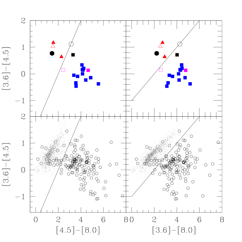
Figure 7: Bottom panels display in the IRAC color-color diagrams the variable stars detected by McQuinn et al. (2007) (small dot symbols) and young HII regions (the open circles; these are sources in the catalogue of Verley et al. (2007) with H$\alpha$ counterpart and not classified as variables) . Only 3$\%$ of variable stars lie to the right of the continuous line. In the upper panels we show the same IRAC colors but for our source sample. Open symbols are sources where no CO has been detected, filled symbols are sources with CO detection. Triangles are for variable stars. The open circle is for source 4, with uncertain classification. Squares are for sources from 5 to 19, i.e. HII regions with 24 $\mu$m counterparts. The filled dot is for s20, a variable star coincident with an HII region without 24 $\mu$m emission.

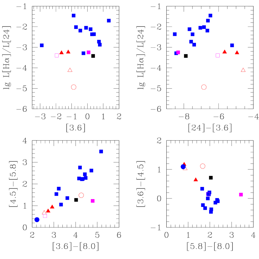
Figure 8: Other colours…same symbols as in previous Figure. The source with the highest flux at 3.6 $\mu$m is s14.

The two lines in Figure 7 have slopes 1 and 0.5 respectively and separate the region populated by evolved stars. Only about 3$\%$ of the evolved stars lie to the right of the lines (about 10$\%$ of the IR selected HII regions lie to their left). The sources considered in this paper well represent the two distributions. Our HII regions with a detectable CO, 24 $\mu$m and H$\alpha$ emission lie in a well defined region and not in the upper left corner where most of the evolved stars lie. Close to the dividing line we find s17, an embedded HII region candidate without H$\alpha$ and very low UV fluxes, and s16, the HII region devoid of CO. We cannot exclude that s16, s17 host an evolved star which did not meet the classification schemes used (actually they are both within a few parsec of a non-point source variable according to Hartman et al. (2006)). The probability for an AGB star to encounter a SF region is low in the solar neighborhood (Kastner & Myers 1994) but it can be appreciable along spiral arms and filaments. The colours of s20, an evolved HII region with no 24 $\mu$m counterpart and associated to an evolved variable star has IRAC colors similar to variable stars.

Figure 9: Star symbols in the lower panels are for 24 $\mu$m sources with no H$\alpha$ counterpart which have been not identified by McQuinn et al. (2007) as variable stars. Filled triangles in the upper panels are sources in Verley et al. (2007) catalogue which host variable stars according to McQuinn et al. (2007).

In Figure 8 we display other variables and colors, even outside the IRAC range. In each panel the young HII regions where dust and CO emission have been detected occupy well defined areas. For example all of them except one (s14) have the 3.6 $\mu$m magnitude above -1 and have [24]-[3.6]$<-6.5$. Similarly their IRAC color [5.8]-[8.0] is $>1.6$. There is also a nice correlation between the [4.5]-[5.8] color and the [3.6]-[8.0] color with the young HII regions where dust and CO emission have been detected lying at [4.5]-[5.8]$>1$. Triangles in the upper panels of Figure 9 indicate the colors of 24 $\mu$m sources in the catalogue of Verley et al. (2007) with no H$\alpha$ counterpart which “host” a variable star i.e. at least one classified variable is located within the 24 $\mu$m emission boundary. Only 25 out of 125 sources in the catalogue of Verley et al. (2007) with no H$\alpha$ counterpart and detected in IRAC bands have been classified as variable stars. Most of these lie to the left of the lines drawn in Figure 9. Variable sources which lie to the right of the line may contain both an evolved star and an embedded HII region. In the bottom panels we show sources with no H$\alpha$ counterpart according to the catalogue of Verley et al. (2007) not associated to known variable stars. The number of these sources which lie to the left of the line exceed by far the percentage expected if these sources have similar colors to the visible HII regions. Either embedded stars occupy a wider area of the IRAC color-color diagram than HII regions or there are unidentified AGBs, variables in crowded regions which escaped the classification by McQuinn et al. (2007). The majority of sources to the right of the line are good candidate for being young star forming regions. Only 5 of these sources are associated with known GMCs. The associated molecular clouds might be of smaller mass, like the ones detected in the CO survey presented here.

5 The cluster birthline test

To verify the young age of our sources we will check if they lie close to the cluster birthline, which is the line in the L_bol–L_bol/L_Hα plane around which young clusters lie (Corbelli et al. 2009). Older clusters should be located above the birthline because of the faster fading of the H$\alpha$ luminosity compared to the bolometric luminosity. Leakage of ionizing photons or the ejection or the delayed formation of massive stars can also move the clusters above the birthline. In Figure 10 we show with star symbols the birthline relative to a stochastically sampled universal IMF with a Salpeter slope -2.35 at the high-mass end. Stochasticity allows a spread in the values of L_bol/L_Hα for a given L_bol: for a given bolometric luminosity we can have a fully populated IMF up to a certain mass M_max, or an IMF populated only up to M${}_{*}<$ M_max, plus a brighter outlier. The errorbars in each bin indicate the dispersion due to bright outliers that can form for the given L_bol. The highest simulated L_bol/L_Hα value is for a fully populated IMF case. We see that there are two sources (s12,s16) which are clearly above the upper 3-$\sigma$ boundary. These might be more evolved sources or leaking ionizing radiation. Since we have not found CO emission from s16, it is likely that it is an evolving source. The source s12 is the brightest in the IR and has a strong CO emission: thus, its position can be explained if it is in the process of forming its massive stellar population or if it is leaking ionizing photons. The strong 8 $\mu$m emission places s12 in the upper right corner of the [3.6]-[8.0]–[4.5]-[5.8] color plot. All the other sources cannot be found below the birthline if the IMF assumptions are correct. Our sources are all compatible with a random sampled IMF model including the two sources, s13 and s19, close to the lower boundary which might host outlier stars.

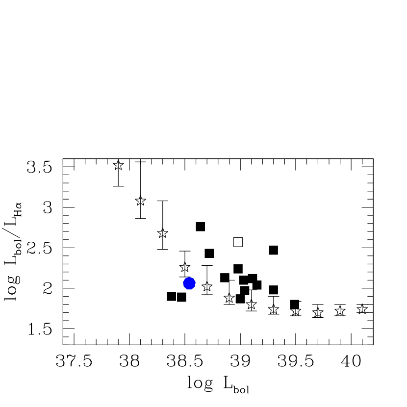
Figure 10: Sources on the cluster birthline. Star symbols indicate the birthline relative to a stochastically sampled universal IMF with their 1-$\sigma$ dispersion. Open symbols are for sources where no CO has been detected, filled symbols are sources with a CO detection. The filled dot is for s20 which does not have IR emission.

6 Conclusions

We have investigated the nature of faint 24 $\mu$m sources with a weak or no H$\alpha$ counterpart. These could be regions with embedded clusters still associated to molecular gas, or evolved stars with dusty envelopes. To distinguish between these two possibilities, we have used published catalogues of variable stars in M33 and carried out deep observations of the CO J=1-0 and 2-1 line with the IRAM 30-mt telescope to search for molecular gas associated with 20 sources. The main results are:

• Deep pointed CO observations have revealed the presence of CO around 17 of the 20 sources included in our sample. The weakness of the CO lines around most of our sources is indicative of the existence of a large population of faint CO clouds in M33. This is in agreement with the results of the CO survey of Gratier et al. (2010) and with the steeper molecular mass spectrum relative to our Galaxy (Blitz & Rosolowsky 2005).

• The estimate of cloud masses is uncertainsince our pointed observations are deeper than any existing CO map. Considering clouds in virial equilibrium and a weak radial dependence of the CO-to-H₂ conversion factor, we find molecular gas masses in the range $10^{4}$ – $10^{5}$ M_⊙. In this case, cloud sizes agree on average with those predicted by the size-linewidth relation of the Milky Way and resolved GMCs in other galaxies, but have large dispersions. We have also estimated limits to molecular gas masses and sizes in the case where cloud outer envelopes are in pressure equilibrium with the surrounding medium. This model reproduces the observed size-linewidth relation correctly if gravitationally bound cloud cores are a factor 4 smaller in size than the outer envelopes.

• The intrinsic CO J=2-1 to J=1-0 line ratio is generally small, $\sim$0.4, if one makes the assumption that clouds are within a few parsecs from the beam center. The CO lines are weaker at the location of evolved stars than around star forming regions, as is the H$\alpha$ and 70 $\mu$m emission. Stellar clusters associated to clouds in our sample are young since they lie along the cluster birthline.

• In the IRAC color-color diagrams AGB variable stars and HII regions occupy distinct areas even though there is some overlap: most of the AGBs have [3.6]-[4.5] color in the range 0 to 1.5 and lie around a line of slope 0.5 in the [3.6]-[8.0]–[3.6]-[4.5] plane. Most of the 24 $\mu$m sources associated to HII regions have higher values for the [4.5]-[8.0] or [3.6]-[8.0] color than variable stars. The IRAC colors of our 20 selected sources are consistent with these distributions. They show a linear correlation between the [4.5]-[5.8] color and the [3.6]-[8.0] color with the AGBs having the lowest values. The IRAC colors confirm the presence of AGBs in 4 sources of our sample whose variability was previously detected either in infrared or optical surveys.

• Using IRAC color-color diagrams we also predict that in the sample of 24 $\mu$m sources without H$\alpha$ counterpart there are still unidentified evolved stars other than young clusters. The young clusters might lack H$\alpha$ emission because they are of small mass or because they are very compact, and deeply embedded. Additional sensitive CO observations and high resolution far-infrared images will help to identify unambiguously the properties of the young star forming sites in M33.