Geometry of perturbed Gaussian states and quantum estimation

Abstract

We address the nonGaussianity (nG) of states obtained by weakly perturbing a Gaussian state and investigate the relationships with quantum estimation. For classical perturbations, i.e. perturbations to eigenvalues, we found that nG of the perturbed state may be written as the quantum Fisher information (QFI) distance minus a term depending on the infinitesimal energy change, i.e. it provides a lower bound to statistical distinguishability. Upon moving on isoenergetic surfaces in a neighbourhood of a Gaussian state, nG thus coincides with a proper distance in the Hilbert space and exactly quantifies the statistical distinguishability of the perturbations. On the other hand, for perturbations leaving the covariance matrix unperturbed we show that nG provides an upper bound to the QFI. Our results show that the geometry of nonGaussian states in the neighbourhood of a Gaussian state is definitely not trivial and cannot be subsumed by a differential structure. Nevertheless, the analysis of perturbations to a Gaussian state reveals that nG may be a resource for quantum estimation. The nG of specific families of perturbed Gaussian states is analyzed in some details with the aim of finding the maximally non Gaussian state obtainable from a given Gaussian one.

1 Introduction

NonGaussianity (nG) is a resource for the implementation of continuous variable quantum information in bosonic systems [1]. Several schemes to generate nonGaussian states from Gaussian ones have been proposed, either based on nonlinear interactions or on conditional measurements [2, 3, 4, 5, 6, 7, 8, 9, 10, 11, 12, 13, 14, 15, 17, 18, 19, 20, 21, 16, 22, 23, 24, 25]. In many cases the effective nonlinearity is small, and so it is the resulting nG. It is thus of interest to investigate the nG of states in the neighbourhood of a Gaussian state, i.e. the nG of slightly perturbed Gaussian states. Besides the fundamental interest [26] this also provides a way to assess different deGaussification mechanisms, as well as nG itself as a resource for quantum estimation. Indeed, in an estimation problem where the variation of a parameter affects the Gaussian character of the involved states one may expect the amount of nG to play a role in determining the estimation precision.

Quantum estimation deals with situations where one tries to infer the value of a parameter $\lambda$ by measuring a different quantity $X$, which is somehow related to $\lambda$. This often happens in quantum mechanics and quantum information where many quantities of interest, e.g. entanglement [27, 28], do not correspond to a proper observable and should be estimated from the measurement of one or more observable quantities [29]. Given a set $\{\varrho_{\lambda}\}$ of quantum states parametrized by the value of the quantity of interest, an estimator $\hat{\lambda}$ for $\lambda$ is a real function of the outcomes of the measurements performed on $\varrho_{\lambda}$. The quantum Cramer-Rao theorem [30, 31, 32, 33] establishes a lower bound for the variance ${\mathrm{Var}}(\lambda)$ of any unbiased estimator, i.e. for the estimation precision, ${\mathrm{Var}}(\lambda)\geq(MH(\lambda))^{-1}$ in terms of the number of measurements $M$ and the so-called quantum Fisher information (QFI), which captures the statistical distinguishability of the states within the set. Indeed, the QFI distance itself is proportional to the Bures distance $d^{2}_{B}(\varrho_{1},\varrho_{2})=2[1-F(\varrho_{1},\varrho_{2})]$, $F(\varrho_{1},\varrho_{2})=\hbox{Tr}[\sqrt{\sqrt{\varrho_{1}}\varrho_{2}\sqrt{\varrho_{2}}}]$ being the fidelity, between states corresponding to infinitesimally close values of the parameter, i.e., in terms of metrics, $H(\lambda)=4\,g_{\lambda}=2\sum_{nm}(\varrho_{n}+\varrho_{m})^{-1}\left|\langle\psi_{m}|\partial_{\lambda}\varrho_{\lambda}|\psi_{n}\rangle\right|^{2}$ where $d^{2}_{B}(\varrho_{\lambda+d\lambda},\varrho_{\lambda})=g_{\lambda}\,d\lambda^{2}$, and we have used the eigenbasis $\varrho_{\lambda}=\sum_{n}\varrho_{n}|\psi_{n}\rangle\langle\psi_{n}|$.

2 Gaussian states and a measure of non Gaussianity

Let us consider a single-mode bosonic system described by the mode operator $a$ with commutation relations $[a,a^{\dagger}]=1$. A quantum state $\varrho$ is fully described by its characteristic function $\chi[\varrho](\lambda)=\hbox{Tr}[\varrho\>D(\lambda)]$ where $D(\lambda)=\exp\{\lambda a^{{\dagger}}-\lambda^{*}a\}$ is the displacement operator. The canonical operators are given by $q=(a+a^{{\dagger}})/\sqrt{2}$ and $p=(a-a^{{\dagger}})/\sqrt{2}i$ with commutation relations given by $[q,p]=i$. Upon introducing the vector $\boldsymbol{R}=(q,p)^{T}$, the covariance matrix $\boldsymbol{\sigma}_{\!\varrho}$ and the vector of mean values $\boldsymbol{X}_{\!\varrho}$ of a quantum state $\varrho$ are defined as $\sigma_{kj}=\frac{1}{2}\langle R_{k}R_{j}+R_{j}R_{k}\rangle_{\varrho}-\langle R_{j}\rangle_{\varrho}\langle R_{k}\rangle_{\varrho}$ and ${X}_{j}=\langle R_{j}\rangle_{\varrho}$, where $\langle O\rangle_{\varrho}=\hbox{Tr}[\varrho\,O]$ is the expectation value of the operator $O$ on the state $\varrho$. A quantum state is said to be Gaussian if its characteristic function has a Gaussian form. Once the CM and the vectors of mean values are given, a Gaussian state is fully determined.

The amount of nG $\delta[\varrho]$ of a quantum state $\varrho$ may be quantified by the quantum relative entropy [34] ${\sf S}(\varrho\rVert\tau_{\varrho})=\hbox{Tr}[\varrho(\log\varrho-\log\tau)]$ between $\varrho$ and its reference Gaussian state $\tau_{\varrho}$, which is a Gaussian state with the same covariance matrix $\boldsymbol{\sigma}$ as $\varrho$. As for its classical counterpart, the Kullback-Leibler divergence, it can be demonstrated that $0\leq{\sf S}(\varrho\rVert\tau)<\infty$ when it is definite, i.e. when $\mathrm{supp}\>\varrho\subseteq\>\mathrm{supp}\>\tau$. In particular ${\sf S}(\varrho\rVert\tau_{\varrho})=0$ iff $\varrho\equiv\tau_{\varrho}$ [35, 36]. Since $\tau_{\varrho}$ is Gaussian $\hbox{Tr}[(\tau_{\varrho}-\varrho)\>\log\tau_{\varrho}]=0$, i.e. ${\sf S}(\varrho\rVert\tau_{\varrho})={\sf S}(\tau_{\varrho})-{\sf S}(\varrho)$ and we may write $\delta[\varrho]={\sf S}(\tau_{\varrho})-{\sf S}(\varrho)$ where ${\sf S}(\varrho)=-\hbox{Tr}[\varrho\>\log\varrho]$ is the von Neumann entropy of $\varrho$. Finally, since the von Neumann entropy of a single-mode Gaussian state may be written as $h(\sqrt{\det\boldsymbol{\sigma}_{\!\varrho}})$ where $h(x)=(x+\frac{1}{2})\log(x+\frac{1}{2}))-(x-\frac{1}{2})\log(x-\frac{1}{2})$ we have

$$\delta[\varrho]=h(\sqrt{\det\boldsymbol{\sigma}_{\!\varrho}})-{\sf S}(\varrho)\,.$$ (1)

A generic single-mode Gaussian state may be written as $\tau=U_{\scriptstyle\!S}\,\nu\,U^{\dagger}_{\scriptstyle\!S}$ where $U_{\scriptstyle\!S}$ is a symplectic operation i.e. a unitary $U_{\scriptstyle\!S}=\exp{-iH}$ resulting from a Hamiltonian $H$ at most quadratic in the field operators, and $\nu$ is a chaotic (maximum entropy) state with $n_{\nu}=\hbox{Tr}[\nu\,a^{\dagger}a]$ average thermal quanta, i.e. $\nu=\sum_{k}p_{k}|k\rangle\langle k|$ , $p_{k}=n_{\nu}^{k}/(1+n_{\nu})^{1+k}$ in the Fock number basis.

3 Classical perturbations to a Gaussian state

An infinitesimal perturbation of the eigenvalues $p_{k}$ of a Gaussian state $\tau$, i.e. $p_{k}\rightarrow p_{k}+dp_{k}$ results in a perturbed state $\varrho=\sum_{k}(p_{k}+dp_{k})U_{\scriptstyle\!S}|k\rangle\langle k|U^{\dagger}_{\scriptstyle\!S}$ which, in general, is no longer Gaussian. Since the nG of a state is invariant under symplectic operations we have $\delta[\varrho]=\delta[\eta]$ where $\eta=U^{{\dagger}}_{\scriptstyle\!S}\!\varrho\,U_{\scriptstyle\!S}=\sum_{k}(p_{k}+dp_{k})|k\rangle\langle k|$ is diagonal in the Fock basis. The Gaussian reference $\tau_{\eta}$ of $\eta$ is a thermal state with $n_{\eta}=n_{\nu}+dn=\sum_{k}k\,(p_{k}+dp_{k})$ average quanta and the nG may be evaluated upon expanding both terms in $\delta[\eta](=\delta[\varrho])$ up to the second order,

$$\delta[\varrho]=\sum_{k}\frac{dp_{k}^{2}}{2p_{k}}-\frac{dn^{2}}{2n_{\nu}(1+n_{\nu})}\,.$$ (2)

NonGaussianity of perturbed states is thus given by the sum of two contributions. The first term is the Fisher information of the probability distribution $\{p_{k}\}$, which coincides with the classical part of the Bures distance in the Hilbert space. The second term is a negative contribution expressed in terms of the infinitesimal change of the average number of quanta. When traveling on surfaces at constant energy the amount of nG coincides with a proper distance in the Hilbert space and, in this case, it has a geometrical interpretation as the infinitesimal Bures distance. At the same time, since Bures distance is proportional to the QFI one, it expresses the statistical distinguishability of states, and we conclude that moving out from a Gaussian state towards its nonGaussian neighbours is a resource for estimation purposes. Similar conclusions can be made when comparing families of perturbations $\{dp\}$ corresponding to the same infinitesimal change of energy $dn^{2}$: in this case the different amounts of nG induced by the perturbations are quantified by the Bures distance minus a constant term depending on $dn^{2}$ and the initial thermal energy $n_{\nu}$, i.e. the intial purity $\mu\equiv\hbox{Tr}[\varrho^{2}]=\hbox{Tr}[\tau^{2}]=(2n_{\nu}+1)^{-1}$ We summarize the above statements in the following

Theorem 1

If $\tau_{\lambda}$ is a Gaussian state and an infinitesimal variation of the value of $\lambda$ drives it into a state $\varrho_{\lambda+d\lambda}$ with the same eigenvectors, then the QFI distance is equal to the nG $\delta[\varrho_{\lambda+d\lambda}]$ plus a term depending both on the infinitesimal variation of energy $dn^{2}$ and on the initial purity

$$H(\lambda)d\lambda^{2}=\delta[\varrho_{\lambda+d\lambda}]+\frac{2\,\mu^{2}dn^{2}}{1-\mu^{2}}\>.$$

In particular, for perturbations that leave the energy unperturbed the nG of the perturbed state coincides with the QFI distance, whereas, in general, it provides a lower bound. $\square$

3.1 Examples of finite perturbations

In order to explore specific directions in the neighbourhood of a Gaussian state $\tau$ let us write the perturbation to the eigenvalues as $dp_{k}=\epsilon\mu_{k}$ where $\{\mu_{k}\}$ is a given distribution. In this case the nG of the perturbed state is given by

$$\delta[\varrho]=\epsilon^{2}\,\left(\sum_{k}\frac{(p_{k}-\mu_{k})^{2}}{2p_{k}}-\frac{\Delta n_{\mu}^{2}}{2n_{t}(1+n_{t})}\right)+O(\epsilon^{3})\,,$$ (3)

where $\Delta n_{\mu}=\sum_{k}(p_{k}-\mu_{k})\langle k|a^{\dagger}a|k\rangle$ Let us now consider the families of states generated by the convex combination $\varrho=(1-\epsilon)\tau+\epsilon\varrho_{\mu}$ of the Gaussian states $\tau$ with a the target state $\varrho_{\mu}=\sum_{k}\mu_{k}U_{\scriptstyle\!S}|k\rangle\langle k|U^{\dagger}_{\scriptstyle\!S}$, which itself is obtained by changing the eigenvalues $p_{k}$ of the initial Gaussian state to $\mu_{k}$. Again we exploit invariance of $\delta[\varrho]$ under symplectic operations and focus attention to the diagonal state $\eta=U_{\scriptstyle\!S}^{{\dagger}}\varrho U_{\scriptstyle\!S}=(1-\epsilon)\eta+\epsilon\,\eta_{\mu}$ which has the same nG of $\varrho$. This is the generalization to a finite perturbation of the analysis reported in the previous Section, and it is intended as a mean to find the maximally nonGaussian state obtainable starting from a given Gaussian. NonGaussianity of this kind of states can be written as $\delta[\eta]=S(\tau_{\eta})-S(\eta)=h[n_{\eta}+1/2]-H[q^{(\epsilon)}]$, where $H[q^{(\epsilon)}]=-\sum_{k}q^{(\epsilon)}_{k}\log q^{(\epsilon)}_{k}$ denotes the Shannon entropy of the distribution $q_{k}^{(\epsilon)}=(1-\epsilon)p_{k}+\epsilon\mu_{k}$ and $n_{\eta}=\hbox{Tr}[\eta\,a^{{\dagger}}a]=(1-\epsilon)n_{t}+\epsilon\,n_{\mu}$ is the average number of quanta of $\eta$. Notice that for a thermal state with $n_{t}$ quanta we have ${H}[p]=h[n_{t}+1/2]$. By using the concavity of the Shannon entropy we obtain an upper bound for the nG

$$\delta[\eta]\leq h[n_{\eta}+1/2]-h[n_{t}+1/2]+\epsilon\Big{(}h[n_{t}+1/2]-H[\mu]\Big{)}$$ (4)

In particular, if the two distributions have the same number of quanta, $n_{\mu}=n_{t}$, and thus $n_{t}=n_{\eta}$, the bound on $\delta[\eta]$ only depends on the difference between the entropy of the initial and target distributions.

Let us now consider perturbations towards some relevant distributions i.e. Poissonian $\mu_{k}^{(p)}=\frac{n_{\mu}^{k}}{k!}e^{-n_{\mu}}$, thermal $\mu_{k}^{(t)}$, and Fock $\mu_{k}^{(d)}=\delta_{k,n_{\mu}}$ and evaluate the nG of states obtained as convex combination of a thermal state with $n_{t}$ quanta and a diagonal quantum state with a Poissonian, thermal or Fock distributions and $n_{\mu}$ quanta.

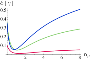
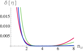
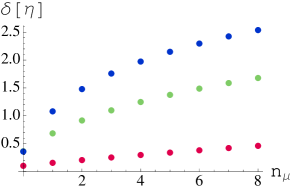
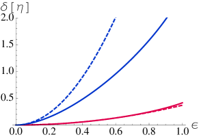
Figure 1: NonGaussianity $\delta[\eta]$ as a function of the energy of the target state $n_{\mu}$ , with $n_{t}=4$ and for different values of $\epsilon=0.3,0.7,0.9$ (red, green and blue, respectively) for Poissonian target (upper left panel), thermal (upper right) and Fock (lower left). The lower right panel shows the nG $\delta[\eta]$ as a function of $\epsilon$, with $n_{\mu}=n_{t}=4$ and for convex combination with a Poissonian (red) and a Fock (blue) state. Dashed lines correspond to the expansion of nG at the second order in $\epsilon$, as obtained in Eq. (3) for the corresponding perturbations.

In Fig. 1 we plot the nG of the convex combination $\varrho$ as a function of $n_{\mu}$ for different values of $\epsilon$: If we consider the convex combination with a Fock state, the nG simply increases monotonically with the energy of the added state. For combinations with Poissonian and thermal distributions we have a maximum for $n_{\mu}\rightarrow 0$, then a local minimum (which for the thermal distribution corresponds trivially to $\delta[\varrho]=0$) for $n_{\mu}=n_{t}$, and then the nonG increases again for higher values of $n_{\lambda}$. This implies that in order to increase nG the best thing to do is to perturb the initial Gaussian either with a highly excited state $n_{\mu}\gg 1$ or with the vacuum state $|0\rangle\langle 0|$. If we choose $n_{\varrho}=n_{\mu}=n_{t}$ we know from Eq. (2) that nG for small perturbations is equivalent to the Bures infinitesimal distance between the two probability distributions ${\mu_{k}}$ and ${p_{k}}$. In Fig. 1d we show the nG as a function of $\epsilon$: As it is apparent from the plot the nG obtained by adding a Fock state is always much larger that the one for a Poissonian profile. We observe that in the latter case the expansion at the second order obtained in Eq. (3) is still accurate for values of $\epsilon$ approaching $1$, while it fails to be accurate for $\epsilon\gtrsim 0.2$ for a Fock state, becoming an upper bound on the exact amount of nG. We have also investigated what happens by considering a target distribution randomly chosen on a finite subspace of the infinite Hilbert space: Again we have obtained that, at fixed energy of the target state, perturbing with a Fock state yields the biggest increase of nG. This may be easily generalized to a system of $d$ bosonic modes, where the most general Gaussian state is described by $d(2d+3)$ independent parameters.

4 Perturbations at fixed covariance matrix

Gaussian states are known to be extremal state at fixed covariance matrix for several relevant quantities, e.g. channel capacities and entanglement measures [37]. Therefore, one may wonder whether perturbing a Gaussian state at fixed covariance matrix may be quantified in convenient way for the purposes of quantum estimation. This indeed the case: the nG provides an upper bound to the QFI distance at fixed covariance matrix and thus have an operational interpretation in terms of statistical distinguishability. This is more precisely expressed by the following theorem [1]

Theorem 2

If $\tau_{\lambda}$ is a Gaussian state and an infinitesimal variation of the value of $\lambda$ drives it into a state $\varrho_{\lambda+d\lambda}$ with the same covariance matrix, then the nG $\delta[\varrho_{\lambda+d\lambda}]$ provides an upper bound to the QFI distance

$$H(\lambda)d\lambda^{2}\leq\delta[\varrho_{\lambda+d\lambda}]\>.$$

Proof: If $\varrho_{\lambda+d\lambda}$ and $\tau_{\lambda}$ have the same CM then the nG of $\varrho_{\lambda+d\lambda}$, $\delta[\varrho_{\lambda+d\lambda}]={\sf S}(\varrho_{\lambda+d\lambda}||\tau_{\lambda})=\widetilde{H}(\lambda)d\lambda^{2}$, where the so-called Kubo-Mori-Bogolubov information $\widetilde{H}(\lambda)$ [38, 39] provides an upper bound for the quantum Fisher information $H(\lambda)\leq\widetilde{H}(\lambda)$ [40], thus proving the theorem. $\square$

The above theorem says that a larger nG of the perturbed state may correspond to a greater distinguishability from the original one, thus allowing a more precise estimation. Of course, this is not ensured by the theorem, which only provides an upper bound to the QFI. One may wonder that when $\varrho_{\lambda+d\lambda}$ is itself a Gaussian state the theorem requires $H(\lambda)=0$, i.e. no reliable estimation is possible. Indeed, this should be the case, since Gaussian states are uniquely determined by the first two moments and thus the requirement that the perturbed $\tau_{\lambda+d\lambda}$ and the original state $\tau_{\lambda}$ are both Gaussian and have the same covariance matrix implies that they are actually the same quantum state.

5 Conclusions

In conclusion, we have addressed the nG of states obtained by weakly perturbing a Gaussian states and have investigated the relationships with quantum estimation. We found that nG provides a lower bound to the QFI distance for classical perturbations, i.e. perturbations to eigenvalues leaving the eigenvectors unperturbed, and an upper bound for perturbations leaving the covariance matrix unperturbed. For situations where the CM is changed by the perturbation we have no general results. On the other hand, it has been already shown that non-Gaussian states improve quantum estimation of both unitary perturbations as the displacement and the squeezing parameters [41] and nonunitary ones as the loss parameter of a dissipative channel [42]. Overall, our results show that the geometry of nonGaussian states in the neighbourhood of a Gaussian state is definitely not trivial and cannot be subsumed by a differential structure. Despite this fact, the analysis of perturbations to a Gaussian state may help in revealing when, and to which extent, nG is a resource for quantum estimation. We have also analyzed the nG of specific families of perturbed Gaussian states with the aim of finding the maximally non Gaussian state obtainable from a given Gaussian one.

References

References

- [1] M. G. Genoni, M. G. A. Paris, Phys. Rev. A 82, 052341 (2010).
- [2] S. Olivares, M. G. A. Paris, J. Opt. B 7, S616 (2005).
- [3] M. S. Kim, J. Phys. B, 41, 133001 (2008).
- [4] A. I. Lvovsky, H. Hansen, T. Aichele, O. Benson, J. Mlynek, and S. Schiller, Phys. Rev. Lett. 87, 050402 (2001).
- [5] J. Wenger, R. Tualle-Brouri, P. Grangier, Phys. Rev. Lett. 92, 153601 (2004).
- [6] A. Zavatta, S. Viciani, M. Bellini, Phys. Rev. A. 70, 053821 (2004).
- [7] A. Ourjoumtsev, R. Tualle-Brouri, J. Laurat, and P. Grangier, Science 312, 83 (2006).
- [8] J.S. Neergard-Nielsen, B. M. Nielsen, C. Hettich, K. Molmer and E. S. Polzik, Phys. Rev. Lett. 97, 083604 (2007).
- [9] A. Ourjoumtsev, H. Jeong, R. Tualle-Brouri, and P. Grangier, Nature 448, 784 (2007).
- [10] A. Zavatta, V. Parigi, and M. Bellini, Phys. Rev. A 75, 052106 (2007).
- [11] V. Parigi, A. Zavatta, M.S. Kim, and M. Bellini, Science, 317, 1890 (2007).
- [12] A. Zavatta, V. Parigi, M. S. Kim, H. Jeong, and M. Bellini, Phys. Rev. Lett. 103, 140406 (2009).
- [13] A. Ourjoumtsev, F. Ferreyrol, R. Tualle-Brouri, and P. Grangier, Nature Phys. 5, 189 (2009).
- [14] A. Ourjoumtsev, A. Dantan, R. Tualle-Brouri, and P. Grangier, Phys. Rev. Lett. 98, 030502 (2007).
- [15] H. Takahashi, J. S. Neergaard-Nielsen, M. Takeuchi, M. Takeoka, K. Hayasaka, A. Furusawa and M. Sasaki, Nature Phot. 4 178 (2010).
- [16] M. Sasaki and S. Suzuki, Phys. Rev. A, 73 (2006) 043807.
- [17] V. D’Auria, C. de Lisio, A. Porzio, S. Solimeno, J. Anwar and M. G. A. Paris, Phys. Rev. A, 81 (2010) 033846.
- [18] A. Chiummo, M. De Laurentis, A. Porzio, S. Solimeno and M. G. A. Paris, Opt. Expr., 13 (2005) 948.
- [19] C. Silberhorn, P. K. Lam, O. Weiß, F. König, N. Korolkova, and G. Leuchs, Phys. Rev. Lett., 86, 4267 (2001).
- [20] O. Glöckl, U. L. Andersen and G. Leuchs, Phys. Rev. A 73, 012306 (2006) .
- [21] T. Tyc and N. Korolkova, New J. Phys., 10, 023041 (2008).
- [22] M. Genoni, F. A Beduini, A. Allevi, M. Bondani, S. Olivares, M. G. A. Paris, Phys. Scr. T140, 014007 (2010).
- [23] A. Allevi, A. Andreoni, M. Bondani, M. G. Genoni and S. Olivares, Phys. Rev. A 82, 013816 (2010).
- [24] A. Allevi, A. Andreoni, F. A. Beduini, M. Bondani, M. G. Genoni, S. Olivares, M. G. A. Paris, EPL 92, 20007 (2010).
- [25] M. Barbieri, N. Spagnolo, M. G. Genoni, F. Ferreyrol, R. Blandino, M. G. A. Paris, P. Grangier, R. Tualle-Brouri, Phys. Rev. A 82, 063833 (2010).
- [26] M. Allegra, P. Giorda, M. G. A. Paris, Phys. Rev. Lett. 105, 100503 (2010).
- [27] M. Genoni, P. Giorda, M. G. A. Paris, Phys. Rev. A 78, 032303 (2008).
- [28] G. Brida, I. Degiovanni, A. Florio, M. Genovese, P. Giorda, A. Meda, M. G. Paris, A. Shurupov, Phys. Rev. Lett. 104, 100501 (2010).
- [29] M. G A Paris, Int. J. Quant. Inf. 7, 125 (2009).
- [30] S. L. Braunstein, C. M. Caves, Phys. Rev. Lett. 72 3439 (1994); S. L. Braunstein, C. M. Caves, G. J. Milburn, Ann. Phys. 247, 135 (1996).
- [31] A. Fujiwara, METR 94-08 (1994).
- [32] S. Amari and H. Nagaoka, Methods of Information Geometry, Trans. Math. Mon. 191, AMS (2000).
- [33] D. C. Brody, L. P. Hughston, Proc. Roy. Soc. Lond. A 454, 2445 (1998); A 455, 1683 (1999).
- [34] M. G. Genoni, M. G. A. Paris, K. Banaszek, Phys. Rev. A 78, 060303(R) (2008).
- [35] B. Schumacher, M. D. Westmoreland, Relative Entropy in Quantum Information Theory in AMS Cont. Math., 305 (2002).
- [36] V. Vedral, Rev. Mod. Phys. 74, 197 (2002).
- [37] M. M. Wolf, G. Giedke, and J. I. Cirac, Phys. Rev. Lett. 96, 080502 (2006).
- [38] X. B. Wang, T. Hiroshima, A. Tomita, M. Hayashi, Phys. Rep. 448, 1 (2007).
- [39] S. Amari, H. Nagaoka, Methods of information geometry (AMS & Oxford University Press, 2000).
- [40] D. Petz, Lin. Alg. Appl. 224, 81 (1996).
- [41] M. G. Genoni, C. Invernizzi and M. G. A. Paris, Phys. Rev. A 80, 033842 (2009).
- [42] G. Adesso, F. Dell’Anno, S. De Siena, F. Illuminati, L. A. M. Souza, Phys. Rev. A 79, 040305(R) (2009).