An overview of the coupled atmosphere-wildland
fire model WRF-Fire

1 Introduction

Wildland fire is a complicated multiscale process. Fortunately, a practically important range of wildland fire behavior can be captured by the coupling of a mesoscale weather model with a simple 2D fire spread model Clark et al. (1996a, b). Weather has a major influence on wildfire behavior; in particular, wind plays a dominant role in the fire spread. Conversely, the fire influences the weather through the heat and vapor fluxes from burning hydrocarbons and evaporation. The buoyancy created by the heat from the fire can cause tornadic strength winds, and the wind and the moisture from the fire affect the atmosphere also away from the fire. It is well known that a large fire “creates its own weather.” The correct wildland fire shape and progress result from the two-way interaction between the fire and the atmosphere Clark et al. (1996a, b, 2004); Coen (2005).

1.1 Origins and the current state of the model

WRF-Fire Mandel et al. (2009) combines the Weather Research and Forecasting Model (WRF) Skamarock et al. (2008) with a semi-empirical fire spread model, based on the level-set method. WRF-Fire has grown out of the NCAR’s CAWFE code Clark et al. (1996a, b, 2004); Coen (2005), which consists of the Clark-Hall mesoscale atmospheric model coupled with a tracer-based fire spread model, using the spread rate computed from McArthur’s Noble et al. (1980) and later Rothermel (1972) formula. Although the Clark-Hall model has many good properties, it is a legacy serial code, not supported, and difficult to modify or use with real data, while WRF is a parallel supported community code routinely used for real runs. See Coen and Patton (2010) for a further discussion of their relative merits in the wildland fire application. Patton and Coen (2004) proposed a combination of WRF with the tracer-based model from CAWFE, formulated a road map, and made the important observation that the innermost domain of the weather code, which interacts directly with the fire model, needs to run in the Large Eddy Simulation (LES) mode. Patton ported the tracer-based code to Fortran 90, rewrote the heat flux insertion for WRF variables, and produced a prototype code coupled with WRF, which then served as the foundation of further development. However, instead of using the existing tracer-based code, the fire module in WRF-Fire was developed based on the level-set method Osher and Fedkiw (2003), among other reasons, because the level-set function can be manipulated more easily than tracers for data assimilation. Thus, only the fuel variables and the subroutine for the calculation of the fire spread rate remained from CAWFE.

Since the paper Mandel et al. (2009) was written in 2007, a number of algorithms and other aspects have changed, new features were added, and WRF-Fire has been released as a part of WRF starting with version 3.2 in April 2010 Dudhia (2010); Wang et al. (2010). The latest version of WRF-Fire with new features and fixes which have not made it into the WRF download yet, plus additional visualization tools, guides, and diagnostic utilities, are available from the developers at openwfm.org.

1.2 Computational simulations

While WRF-Fire takes advantage of the CAWFE experience, WRF is quite different from the Clark-Hall atmospheric model and the fireline propagation algorithm is also different. Thus, it needs to be demonstrated that WRF-Fire can deliver similar results as CAWFE, and WRF-Fire needs to be validated against real fires. Kim (2011) has shown that the level set method in the fire module can advect the fire shape correctly, just like the CAWFE tracer code in Clark et al. (2004). Jenkins et al. (2010) studied the role of wind profile on fire propagation speed and the shape of the fireline and demonstrated fireline fingering behavior on ideal examples, as in Clark et al. (1996a, b). Kochanski et al. (2010) compared simulation results with measurements on the FireFlux grass fire experiment Clements et al. (2007). Dobrinkova et al. (2010) simulated a fire in Bulgarian mountains using real meteorological and geographical data, and ideal fuel data. Beezley et al. (2010) simulated a fire in Colorado mountains using real data from online sources. A mesoscale simulation can run faster than real time on a small cluster Jordanov et al. (2011).

1.3 Related work

Wildland fire models range from tools based based on fire spread rate formulas Rothermel (1972, 1983), such as BehavePlus Andrews (2007) and FARSITE Finney (1998), suitable for operational forecasting, to sophisticated 3D computational fluid dynamics and combustion simulations suitable for research and reanalysis, such as FIRETEC Linn et al. (2002) and WFDS Mell et al. (2007). BehavePlus, the PC-based successor of the calculator-based BEHAVE, determines the fire spread rate at a single point from fuel and environmental data; FARSITE uses the fire spread rate to provide a 2D simulation on a PC; while FIRETEC and WFDS require a parallel supercomputer and run much slower than real time.

The level set-method was used for a surface fire spread model in Mallet et al. (2009). Filippi et al. (2009) coupled the atmospheric model, Meso-nh, with fire propagation by tracers. Tiger Mazzoleni and Giannino (2010) uses a 2D combustion model based on reaction-convection-diffusion equations and a convection model to emulate the effect of the fire on the wind. FIRESTAR Morvan and Dupuy (2004) is a physically accurate wildland fire model in two dimensions, one horizontal and one vertical. UU LES-Fire Sun et al. (2009) couples the University of Utah’s Large Eddy Simulator with the tracer-based code from CAWFE. See the survey by Sullivan (2009) for a number of other models.

2 Physical fire model and fuels

The physical model consists of subroutines computing the spread rate and the burn rate, and it is essentially the same as a subset of CAWFE Clark et al. (1996a, b, 2004); Coen (2005), Rothermel (1972), and BEHAVE Andrews (2007).

2.1 Fuel properties

Fuel is characterized by a vector of quantities, which are given at every point of the domain. To simplify the specification of fuel properties, fuels are given as one of 13 Anderson (1982) categories, which are preset vectors of values of the fuel properties above. These values are specified in an input text file, and they can be modified by the user. The user can also specify completely new, custom fuels.

2.2 Fire spread rate

Mathematically, the fire model is posed in the horizontal $(x,y)$ plane. The semi-empirical approach to fire propagation used here assumes that the fire spread rate is given by the modified Rothermel’s formula

$$S=R_{0}\left(1+\phi_{W}+\phi_{S}\right).$$ (1)

The spread rate depends on fuel properties, the wind speed $U$, and the terrain slope $\tan\phi$, exactly as in Rothermel (1972), except that some of the input quantities are metric so they are first converted from metric to English units (lb-ft-min) to avoid changing the numerous constants in the computation from Rothermel (1972); the wind is limited to between $0$ to $30$m/s; the slope is limited to nonnegative values; the fuel mass with moisture is given rather than dry fuel as in Rothermel (1972); and a new category is introduced for chaparral from (Coen et al. 2001, eq. (1)). In either case, the spread rate can be written as

$$S=\max\left\{S_{0},R_{0}+c\min\left\{e,\max\left\{0,U\right\}\right\}^{b}+d\max\left\{0,\tan\phi\right\}\right\},$$ (2)

where $S_{0},R_{0}$,$b,c,d,e$ are fuel-dependent coefficients, which is how the spread rate is represented in WRF-Fire internally. These coefficients are stored for every grid point. At a fixed point on the fireline, denote by $\vec{n}$ the outside normal to the fire region, $\overrightarrow{U}$ the wind vector, and $z$ the terrain height. The normal component of the wind vector, $U=\overrightarrow{U}\cdot\vec{n}$, and the normal component of the terrain gradient, $\tan\phi=\nabla z\cdot\vec{n}$, are used to determine the spread rate, which is interpreted as the spread rate in the normal direction $\vec{n}$.

2.3 Fuel burned and heat released

Each location starts with fuel fraction $F=1$. Once the fuel is ignited at a time $t_{i}$, the fuel fraction decreases exponentially,

$$F\left(t\right)=\exp\left(-\frac{\left({t-t}_{i}\right)}{T_{f}}\right),\quad t>{t_{i}}$$ (3)

where $t$ is the time, $t_{i}$ is the ignition time, $F_{0}$ is the initial amount of fuel, and $T_{f}$ is the time constant of fuel, i.e., the number of seconds for the fuel to burn down to $1/e\approx 0.3689$ of the original quantity. Since the fuel burns down to $0.6$ of the original quantity in $600$s when $w=1000$, we have

$$0.6^{\frac{\left(t-t_{i}\right)}{600}\frac{1000}{w}}=\exp\left(-\frac{\left({t-t}_{i}\right)}{T_{f}}\right),$$

which gives

$$T_{f}=-\frac{600}{1000\ln 0.6}\approx\frac{w}{0.8514}.$$

The input coefficient $w$ is used in WRF-Fire rather than $T_{f}$ for compatibility with existing fuel models and literature

The average sensible heat flux density released in time interval $\left(t,t+\Delta t\right)$ is computed as

$$\phi_{h}=\frac{F\left(t\right)-F\left(t+\Delta t\right)}{\Delta t}\frac{1}{1+M_{f}}w_{\ell}h\quad\text{(J/m}^{2}\text{/s)}$$ (4)

and the average latent heat (i.e., moisture) flux density is given by

$$\phi_{q}=\frac{F\left(t\right)-F\left(t+\Delta t\right)}{\Delta t}\frac{M_{f}+0.56}{1+M_{f}}Lw_{\ell}\quad\text{(J/m}^{2}\text{/s)}$$ (5)

where 0.56 is the estimated mass ratio of the water output from combustion to the dry fuel, and $L=2.5\cdot 10^{6}$ J/kg is the specific latent heat of condensation of water at $0$ ^oC, used for nominal conversion of moisture to heat. This computation is from CAWFE.

3 Mathematical core of the fire model

The model maintains level set function $\psi$, time of ignition $t_{i}$, and the fuel fraction $F$. These quantities are all represented by their values at the centers of the fire mesh cells.

3.1 Fire propagation by the level set method

This section follows Mandel et al. (2009). Denote point on the surface by $\mathbf{x}=\left(x,y\right)$. The burning region at time $t$ is represented by a level set function $\psi=\psi\left(\mathbf{x},t\right)$ as the set of all points $\mathbf{x}$ such that where $\psi\left(\mathbf{x},t\right)\leq 0$. There is no fire at $\mathbf{x}$ if $\psi\left(\mathbf{x},t\right)>0$. The fireline is the set of all points $\mathbf{x}$ such that $\psi\left(\mathbf{x},t\right)=0$. Since on the fireline, the tangential component of the gradient $\nabla\psi$ is zero, the outside normal vector at the fireline is

$$\mathbf{n}=\frac{\nabla\psi}{\left\|\nabla\psi\right\|}.$$ (6)

Now consider a point $\mathbf{x}\left(t\right)$ that moves with the fireline. Then the fire spread rate $S$ at $\mathbf{x}$ in the direction of the normal $\mathbf{n}$ is

$$S=\overrightarrow{n}\cdot\frac{\partial\mathbf{x}}{\partial t}.$$ (7)

From $\psi\left(\mathbf{x}\left(t\right),t\right)=0$ and chain rule,

$$0=\frac{d}{dt}\psi\left(x,y,t\right)=\frac{\partial\psi}{\partial t}+\frac{\partial\psi}{\partial x}\frac{\partial x}{\partial t}+\frac{\partial\psi}{\partial y}\frac{\partial y}{\partial t}=\frac{\partial\psi}{\partial t}+\left\|\nabla\psi\right\|\left(\mathbf{n}\cdot\frac{\partial\mathbf{x}}{\partial t}\right)=\frac{\partial\psi}{\partial t}+S\left\|\nabla\psi\right\|,$$ (8)

so, from (7) and (8), the level set function is governed by the partial differential equation

$$\frac{\partial\psi}{\partial t}+S\left(x\right)\left\|\nabla\psi\right\|=0,$$ (9)

called the level set equation Osher and Fedkiw (2003). The spread rate $S$ is evaluated from (2) everywhere on the domain. Since $S\geq 0$, the level set function does not increase with time, and the fire area cannot decrease, which also helps with numerical stability by eliminating oscillations of $\psi$ in time.

The level set equation is discretized on a rectangular grid with spacing $\left(\triangle x,\triangle y\right)$, called the fire grid. The level set function $\psi$ and the ignition time $t_{i}$ are represented by their values at the centers of the fire grid cells. This is consistent with the fuel data given in the center of each cell also.

To advance the fire region in time, we use Heun’s method (Runge-Kutta method of order $2$),

$$\psi^{n+1/2} =\psi^{n}+\Delta tF\left(\psi^{n}\right)$$

$$\psi^{n+1} =\psi^{n}+\Delta t\left(\frac{1}{2}F\left(\psi^{n}\right)+\frac{1}{2}F\left(\psi^{n+1/2}\right)\right),$$ (10)

The right-hand side $F$ is a discretization of the term $-S\left\|\nabla\psi\right\|$ with upwinding and artificial viscosity, specifically,

$$F\left(\psi\right)=-S\left(\overrightarrow{v}\cdot\overrightarrow{n},\nabla z\cdot\overrightarrow{n}\right)\left\|\overline{\nabla}\psi\right\|+\varepsilon\widetilde{\triangle}\psi,$$

where $\overrightarrow{n}=\nabla\psi/\|\nabla\psi\|$ is computed by central differences and $\overline{\nabla}\psi=\ \left[\overline{\nabla}_{x}\psi,\overline{\nabla}_{y}\psi\right]$ is the upwinded finite difference approximation of $\nabla\psi$ by Godunov’s method (Osher and Fedkiw 2003, p. 58),

$$\overline{\nabla}_{x}\psi=\left\{\begin{array}[c]{c}\overline{\nabla}_{x}^{+}\psi\text{ if }\overline{\nabla}_{x}^{-}\psi\leq 0\text{ and }\overline{\nabla}_{x}^{+}\psi\leq 0,\\ \overline{\nabla}_{x}^{-}\psi\text{ if }\overline{\nabla}_{x}^{-}\psi\geq 0\text{ and }\overline{\nabla}_{x}^{+}\psi\geq 0,\\ 0\text{ if }\overline{\nabla}_{x}^{-}\psi\leq 0\text{ and }\overline{\nabla}_{x}^{+}\psi\geq 0,\\ \text{otherwise }\overline{\nabla}_{x}^{-}\psi\text{ if }\left|\overline{\nabla}_{x}^{-}\psi\right|\geq\left|\overline{\nabla}_{x}^{+}\psi\right|,\\ \quad\quad\quad\quad\quad\overline{\nabla}_{x}^{+}\psi\text{ if }\left|\overline{\nabla}_{x}^{-}\psi\right|\leq\left|\overline{\nabla}_{x}^{+}\psi\right|,\end{array}\right.$$ (11)

where $\nabla_{x}^{+}\psi$ and $\nabla_{x}^{-}\psi$ are the right and left one-sided differences

$$\nabla_{x}^{+}\psi\left(x,y\right) =\frac{\psi\left(x+\triangle x,y\right)-\psi\left(x,y\right)}{\triangle x},$$

$$\nabla_{x}^{-}\psi\left(x,y\right) =\frac{\psi\left(x,y\right)-\psi\left(x-\triangle x,y\right)}{\triangle x},$$

and similarly for $\nabla_{y}^{+}\psi$ and $\nabla_{y}^{-}\psi$. Further,

$$\nabla\psi=\left[\frac{\nabla_{x}^{+}\psi+\nabla_{x}^{-}\psi}{2},\frac{\nabla_{y}^{+}\psi+\nabla_{y}^{-}\psi}{2}\right]$$

is the gradient by central differences, $\varepsilon$ is the scale-free artificial viscosity ($\varepsilon=0.4$ in the computations here), and

$$\widetilde{\triangle}\psi=\nabla_{x}^{+}\psi-\nabla_{x}^{-}\psi+\nabla_{y}^{+}\psi-\nabla_{y}^{-}\psi$$

is the scaled five-point Laplacian of $\psi$.

A numerically stable scheme that includes upwinding, such as Godunov’s method (11), is required to compute $\left\|\nabla\psi\right\|$ in the level set equation (9). However, it seems better to use standard central differences for $\nabla\psi$ in the computation of the normal $\mathbf{n}$ in (6), which is needed to evaluate the normal component of the wind and the slope in (2).

Before computing the one-sided differences up to the boundary, the level set function is extrapolated to one layer of nodes beyond the boundary. However, the extrapolation is not allowed to decrease the value of the level set function under the value at either of the points extrapolated from. For example, when $\left(i,j\right)$ is the last node in the domain in the direction $x,$ the extrapolation

$$\psi_{i+1,j}=\max\left\{\psi_{ij}+\left(\psi_{ij}-\psi_{i-1,j}\right),\psi_{ij},\psi_{i-1,j}\right\},$$

is used, and similarly in the other cases. This modification of the finite difference method serves to avoid numerical instabilities at the boundary. The extrapolation at the boundary effectively implements a free boundary condition. Without the stabilization, a decrease of $\psi$ at a boundary node, which often happens for nonhomogeneous fuels in real data, is amplified by extrapolation and because of upwinding, $\psi$ keeps decreasing at that boundary node forever and developing a large negative spike.

The model does not support fire crossing the boundary of the domain. When $\psi<0$ is detected near the boundary, the simulation terminates. This is not a limitation in practice, because the fire should be well inside the domain anyway for a proper response of the atmosphere.

The ignition time $t_{i}$ in the strip that the fire has moved over in one timestep is computed by linear interpolation from the level set function. Suppose that the point $\mathbf{x}$ is not burning at time $t$ but is burning at time $t+\triangle t$, that is, $\psi\left(\mathbf{x},t\right)>0$ and $\psi\left(\mathbf{x},t+\triangle t\right)\leq 0$. The ignition time at $\mathbf{x}$ satisfies $\psi\left(\mathbf{x},t_{i}\left(\mathbf{x}\right)\right)=0$. Approximating $\psi$ by a linear function in time, we have

$$\frac{\psi\left(\mathbf{x},t_{i}\right)-\psi\left(\mathbf{x},t\right)}{t_{i}\left(\mathbf{x}\right)-t}\approx\frac{\psi\left(\mathbf{x},t+\triangle t\right)-\psi\left(\mathbf{x},t_{i}\right)}{t+\triangle t-t_{i}\left(\mathbf{x}\right)},$$

and we take

$$t_{i}(\mathbf{x})=t+\frac{\psi\left(\mathbf{x},t\right)\triangle t}{\psi\left(\mathbf{x},t\right)-\psi\left(\mathbf{x},t+\triangle t\right)}.$$ (12)

3.2 Computation of the fuel fraction

The fuel fraction is approximated over each fire mesh cell $C$ by integrating (3) over the fire region. Hence, the fuel fraction remaining in cell $C$ at time $t$ is given by

$$1-\frac{1}{\operatorname*{area}\left(C\right)}{\iint\limits_{\genfrac{}{}{0.0pt}{}{\mathbf{x}\in C}{\psi\left(\mathbf{x},t\right)\leq 0}}}1-\exp\left(-\frac{t-t_{i}\left(\mathbf{x}\right)}{T_{f}(\mathbf{x})}\right)d\mathbf{x.}$$ (13)

Once the fuel fraction is known, the heat fluxes are computed from (4) and (5). This scheme has the advantage that the total heat released in the atmosphere after the fuel has completely burned is accurate, regardless of approximations in the computation of the integral (13). We are looking for a scheme that is second order accurate when the whole cell is on fire, exact when no part of the cell $C$ is on fire (namely, returning the value one), and provides a natural transition between these two cases. Just like the standard numerical schemes are exact for polynomials of a certain degree, the guiding principle here is that the scheme should be exact in a collection of (nontrivial) special cases.

While the fuel time $T_{f}$ can be interpolated as constant over the whole cell, the level set function $\psi$ and the ignition time $t_{i}$ must be interpolated more accurately to allow submesh representation of the burning area and gradual release of the heat as the fireline moves over the cell. Then, to compute the integral in (13), the cell $C$ is split into 4 subcells $C_{j}$, and

$${\iint\limits_{\genfrac{}{}{0.0pt}{}{\mathbf{x}\in C}{\psi\left(\mathbf{x},t\right)\leq 0}}1-}\exp\left(-\frac{t-t_{i}\left(\mathbf{x}\right)}{T_{f}(\mathbf{x})}\right)d\mathbf{x=}\sum_{j=1}^{4}{\iint\limits_{\genfrac{}{}{0.0pt}{}{\mathbf{x}\in C_{j}}{\psi\left(\mathbf{x},t\right)\leq 0}}1-}\exp\left(-\frac{t-t_{i}\left(\mathbf{x}\right)}{T_{f}(\mathbf{x})}\right)d\mathbf{x.}$$ (14)

The level-set function $\psi$ is interpolated bilinearly to the vertices of the subcells $C_{j}$, and $T_{f}$ is constant on each $C_{j}$. When the whole cell $C$ is on fire (that is, $\psi\leq 0$ on all four vertices of $C$), $t_{i}$ is interpolated also linearly to the vertices of the subcells $C_{j}$. However, the case when the fireline crosses the cell $C$ requires a special treatment of the ignition time $t_{i}$; $t_{i}\left(\mathbf{x}\right)$ has meaningful value only when the node $\mathbf{x}$ is on nodes on fire, $\psi\left(\mathbf{x}\right)\leq 0$, and $t_{i}\left(\mathbf{x}\right)=0$ on the fireline, i.e., when $\psi\left(\mathbf{x}\right)=0$. Approximating both $\psi$ and $t_{i}$ in the fire region by a linear function suggests interpolating from the relation

$$t_{i}-t=c\psi,$$ (15)

for some $c$. We interpolate on the grid lines between two nodes first. If both nodes are on fire, we interpolate $t_{i}$ bilinearly as before. However, when one cell center is on fire and one not, say $\psi\left(\mathbf{a}_{1}\right)>0$, $\psi\left(\mathbf{a}_{2}\right)<0$,. we find the proportionality constant $c$ in (15) from $t_{i}\left(\mathbf{a}_{2}\right)=c\psi\left(\mathbf{a}_{2}\right)$, and set $t_{i}\left(\mathbf{b}\right)=c\psi\left(\mathbf{b}\right)$ at the midpoint $\mathbf{b}=\left(\mathbf{a}_{1}+\mathbf{a}_{2}\right)/2$. In the case of interpolation to the node $\mathbf{c=}\left(\mathbf{a}_{1}+\mathbf{a}_{2}+\mathbf{a}_{3}+\mathbf{a}_{4}\right)/4$ between nodes $\mathbf{a}_{1},\mathbf{a}_{2},\mathbf{a}_{3},\mathbf{a}_{4}$, we find the proportionality constant $c$ by solving the least squares problem

$$\sum_{\begin{subarray}{c}j=1\\ \psi\left(\mathbf{a}_{j}\right)\leq 0\end{subarray}}^{4}\left|t_{i}\left(\mathbf{a}_{j}\right)-t-c\psi\left(\mathbf{a}_{j}\right)\right|^{2}\rightarrow\min$$

and set again $t_{i}\left(\mathbf{c}\right)=c\psi\left(\mathbf{c}\right)$.

To compute the integral over a subcell $C_{j}$, we first estimate the fraction of the subcell that is burning, by

$$\frac{\operatorname*{area}\left\{(x,y)\in C_{j}:\psi\left(x,y,t\right)\leq 0\right\}}{\operatorname*{area}(C_{j})}\approx\alpha=\frac{1}{2}\left(1-\frac{\sum_{k=1}^{4}\psi\left(\mathbf{x}_{k}\right)}{\sum_{k=1}^{4}\left|\psi\left(\mathbf{x}_{k}\right)\right|}\right),$$ (16)

where $\mathbf{x}_{k}$ are the the corners of the subcell $C_{j}$. The approximation is exact when no part of the subcell $C_{j}$, is on fire, that is, all $\psi\left(\mathbf{x}_{k}\right)\geq 0$ and at least one $\psi\left(\mathbf{x}_{k}\right)>0$; the whole $C_{j}$ is on fire, that is, all $\psi\left(\mathbf{x}_{k}\right)\leq 0$ and at least one $\psi\left(\mathbf{x}_{k}\right)<0$; or the values $\psi\left(\mathbf{x}_{k}\right)$ define a linear function and the fireline crosses the subcell diagonally or it is aligned with one of the coordinate directions.

Next, replace $t\left(\mathbf{x}_{k}\right)$ by $t$ when $\psi\left(\mathbf{x}_{k}\right)>0$ (i.e., the node $\mathbf{x}_{k}$ is not on fire), and compute the approximate fraction of the fuel burned as

$$\alpha\left(1-\exp\left(-\frac{1}{4}\sum_{k=1}^{4}\frac{t_{i}\left(\mathbf{x}_{k}\right)-t}{T_{f}}\right)\right)$$ (17)

This computation is a second-order quadrature formula when the whole cell is burning; it is exact when no part of the cell is burning; and it provides a natural transition between the two. Also, the calculation is accurate asymptotically when the fuel burns slowly and the approximation $\beta$ of the burning area is exact.

Optionally, the fuel fraction remaining is computed first by approximating $\psi$ and $t_{i}$ and by linear functions using finite differences and then integrating analytically, first in the direction orthogonal to the fireline and then parallel to the fireline, thus splitting the fire region in the subcell into trapezoids. This method is exact when $\psi$ and $t_{i}$ are linear functions, but it is more expensive. Accurate calculation of the fuel fraction and thus of the heat flux will be important for the simulation of crown fire, which is ignited when the ground heat flux exceeds a certain threshold value Clark et al. (1996b)).

3.3 Ignition

Typically, a fire starts much smaller than the fire mesh cell size, and both point and line ignition need to be supported. The previous ignition mechanism Mandel et al. (2009) ignited everything within a given distance from the ignition line at once. This distance was required to be at least one or two mesh steps, so that the initial fire is visible on the fire mesh, and the fire propagation algorithm from Sec. 3.1 can catch on. This caused an unrealistically large initial heat flux and an accelerated ignition.

The current ignition scheme achieves submesh resolution and zero-size ignition. A small initial fire is superimposed on the regular propagation mechanism, which then takes over. Drip-torch ignition is implemented as a collection of short ignition segments that grow at one end every time step. Multiple ignitions are supported.

The model is initialized with no fire by choosing the level set function $\psi\left(\mathbf{x},t_{0}\right)=\operatorname*{const}>0$. Consider an initial fire that starts at time $t_{g}$ on a segment $\overline{\mathbf{ab}}$ and propagates in all directions with an initial spread rate $S_{g}$ until distance $r_{g}$ is reached. At the beginning of every time step $t$ such that $t_{g}\leq t\leq t_{g}+r_{g}/S_{g}$, we construct the level-set function of the initial fire,

$$\psi_{i}\left(\mathbf{x},t\right)=\operatorname*{dist}\left(\mathbf{x},\overline{\mathbf{ab}}\right)-S_{g}\left(t-t_{g}\right)$$ (18)

and replace the level-set function of the model by

$$\psi\left(\mathbf{x},t\right):=\min\left\{\psi\left(\mathbf{x},t\right),\psi_{i}\left(\mathbf{x},t\right)\right\}.$$ (19)

For a drip-torch ignition starting from point $\mathbf{a}$ at time $t_{g}$ at velocity $\mathbf{v}$ until time $t_{h}$, the ignition line at time $t$ is the segment $\overline{\mathbf{a},\mathbf{a}+\mathbf{v}\left(\min\left\{t,t_{h}\right\}-t_{g}\right)}$, and (18) becomes

$$\psi_{i}\left(\mathbf{x},t\right)=\operatorname*{dist}\left(\mathbf{x},\overline{\mathbf{a},\mathbf{a}+\mathbf{v}\left(\min\left\{t,t_{h}\right\}-t_{g}\right)}\right)-\min\left\{r_{g},S_{g}\left(t-t_{g}\right)\right\}$$

followed again by (19), at the beginning of every time step $t$ such that

$$t_{g}\leq t\leq t_{h}+r_{g}/S_{g}.$$

The ignition time on newly ignited nodes is set to the arrival time of the fire at the spread rate $S_{g}$ from the nearest point on the ignition segment.

4 Atmospheric model

We summarize some background information about WRF from Skamarock et al. (2008) to the extend needed to understand the coupling with the fire module.

4.1 Variables and equations

The model is formulated in terms of the hydrostatic pressure vertical coordinate $\eta$, scaled and shifted so that $\eta=1$ at the Earth surface and $\eta=0$ at the top of the domain. The governing equations are a system of partial differential equations of the form

$$\frac{d\Phi}{dt}=R\left(\Phi\right),$$ (20)

where $\Phi=\left(U,V,W,\phi^{\prime},\Theta,\mu^{\prime},Q_{m}\right)$. The fundamental WRF variables are $\mu=\mu\left(x,y\right)$, the hydrostatic component of the pressure differential of dry air between the surface and the top of the domain, written in perturbation form $\mu=\overline{\mu}+\mu^{\prime}$, where $\overline{\mu}$ is a reference value in hydrostatic balance; $U=\mu u$, where $u=u\left(x,y,\eta\right)$ is the Cartesian component of the wind velocity in the $x$-direction, and similarly $V$ and $W$; $\Theta=\mu\theta$, where $\theta=\theta\left(x,y,\eta\right)$ is the potential temperature; $\phi=\phi\left(x,y,\eta\right)=\overline{\phi}+\phi^{\prime}$ is the geopotential; and $Q_{m}=\mu q_{m}$ is the moisture contents of the air. The variables in the state $\Phi$ evolved by (20) are called prognostic variables. Other variables computed from them, such as the hydrostatic pressure $p$, the thermodynamic temperature $T$, and the height $z$, are called diagnostic variables. The variables that contain $\mu$ are called coupled. The value of the right-hand side $R\left(\Phi\right)$ is called tendency. See (Skamarock et al. 2008, pp. 7-13) for details and the form of $R$.

The system (20) is discretized in time by the explicit 3rd order Runge-Kutta method

$$\Phi_{1} =\Phi^{t}+\frac{\Delta t}{3}R\left(\Phi^{t}\right)$$

$$\Phi_{2} =\Phi^{t}+\frac{\Delta t}{2}R\left(\Phi_{1}\right)$$

$$\Phi^{t+\Delta t} =\Phi^{t}+\Delta tR\left(\Phi_{2}\right)$$ (21)

where only the third Runge-Kutta step includes tendencies from physics packages, such as the fire module (Skamarock et al. 2008, p. 16). In order to avoid small time steps, the tendency in the third Runge-Kutta step also includes the effect of substeps to integrate acoustic modes.

4.2 Surface schemes

In real cases, non zero sf_sfclay_physics should be selected to enable the surface model, allowing for proper interaction between the atmosphere and the land surface. In idealized cases, users have an option of the basic surface initialization, intended to be used without the surface model, or the full surface initialization (sfc_full_init=1). The latter allows for using all standard land surface models even in idealized cases. For idealized cases with full surface initialization, land surface properties like roughness length, albedo etc., are defined through the land use category. The surface scheme utilizes a gridded array containing the number of landuse category, defined in a text file (LANDUSE.TBL), which specifies the roughness length and other surface properties, both for the real and idealized cases. The land use categories may be also defined directly trough the namelist variables or read in from an external file containing a 2D landuse matrix (see also Sec. 7).

5 Coupling of the fire and the atmospheric models

The terrain gradient is computed from the terrain height at the best available resolution and interpolated to the fire mesh in preprocessing. Interpolating the height and then computing the gradient would cause jumps in the gradient, which affect fire propagation, unless high-order interpolation is used.

In each time step of the atmospheric model, the fire module is called from the third step of the Runge-Kutta method. First the wind is interpolated to a fixed height $z_{f}$ above the terrain (currently, 6.1m following BEHAVE), assuming the wind log profile

$$u\left(z\right)\approx\left\{\begin{array}[c]{cc}\operatorname*{const}\log\frac{z}{z_{0}},&z\geq z_{0},\\ 0&0\leq z\leq z_{0},\end{array}\right.$$

where $z$ is the height above the terrain and $z_{0}$ is the roughness height. For a fixed horizonal location, denote by $z_{1},$ $z_{2},\ldots$ the heights of the centers of the atmospheric mesh cells; these are computed from the geopotential $\phi$, which is a part of the solution. The horizontal wind component $U\left(z_{f}\right)$ is then found by interpolating the values $U\left(z_{0}\right)=0,U\left(z_{1}\right),U\left(z_{2}\right),...$ from the nodes $\log z_{0}$, $\log z_{1},\log z_{2},\ldots$ to $\log z_{f}$; if $z_{f}\leq z_{0}$, we set $U\left(z_{f}\right)=0$. The $V$-component of the wind is interpolated in the same way.

The fire model then makes one time step:

1. If there are any active ignitions, the level-set function is updated and the ignition times of any newly ignited nodes are set following Sec. 3.3.

2. The numerical scheme (10)-(11) for the level set equation (9) is advanced to the next time step.

3. The time of ignition set for any any nodes that were ignited during the time step, from (12).

4. The fuel fraction is updated following Sec. 3.2.

5. The sensible and latent heat flux densities are computed from (4) and (5) in each fire model cell.

The resulting heat flux densities are averaged over the fire cells that make up one atmosphere model cell and inserted into the atmospheric model, which then completes its own time step. The heat fluxes from the fire are inserted into the atmospheric model as forcing terms in the differential equations of the atmospheric model into a layer above the surface, with assumed exponential decay with altitude. Such a scheme is needed because WRF does not support flux boundary conditions. The sensible heat flux is inserted as the tendency of the potential temperature $\theta$, equal to the vertical divergence of the heat flux,

$$\frac{d\left(\mu\theta\right)}{dt}\left(x,y,z\right)=R_{\Theta}\left(\Phi\right)+\frac{\mu\left(x,y\right)\phi_{h}\left(x,y\right)}{\sigma\varrho\left(x,y,z\right)}\frac{\partial}{\partial z}\exp\left(-\frac{z}{z_{ext}}\right),$$

where $R_{\Theta}\left(\Phi\right)$ is the component of the tendency in the atmospheric model equations (20), $\sigma$ is the specific heat of the air, $\varrho\left(x,y,z\right)$ is the density, and $z_{ext}$ is the heat extinction depth, a parameter. The latent heat flux is inserted similarly into the tendency of the vapor concentration $q_{m}$ by

$$\frac{d\left(\mu q_{m}\right)}{dt}\left(x,y,z\right)=R_{Q_{m}}\left(\Phi\right)+\frac{\mu\left(x,y\right)\phi_{q}\left(x,y\right)}{L\varrho\left(x,y,z\right)}\frac{\partial}{\partial z}\exp\left(-\frac{z}{z_{ext}}\right),$$

where $L$ is the specific latent heat of the air.

6 Software structure

6.1 Grids and parallel execution

Parallel computing imposes a significant constraint on user programming technique. WRF uses the RSL parallel infrastructure Michalakes (2000). RSL divides the domain horizontally into patches. Each patch executes in a separate MPI process and is further divided into tiles, which execute in separate OpenMP threads. Communication between tiles is accomplished at the end of OpenMP parallel loop over tiles. The fire grid has refined tiles in the same location as atmospheric grid tiles. The patches are declared in memory with larger bounds than the patch size, and communication between patches is accomplished by HALO calls (actually, includes of generated code), which update a layer of nodes beyond the patch boundary from other patches. The fire module computational code itself is designed to be tile-callable; it executes on a single tile, assuming it can safely read data from a layer of nodes beyond the tile boundary. The communication (OpenMP loops or HALO calls) occurs outside the computational routines; this means that whenever communication is necessary, the fire module must exit, and then continue from the correct code location on the next call.

6.2 Software layers

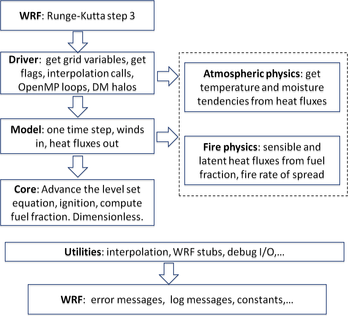
Figure 1: Structure of WRF-Fire software. All physics routines are in the dashed box. The Utilities layer is used by all other components above it.

The fire module software is organized in several isolated layers (Fig. 1). The driver layer serves to interpolate and otherwise translate the variables between WRF and the fire module, and it contains all exchange of data between the tiles in parallel execution. The rest of the code executes on a single tile, assuming that the needed values from neighboring tiles are already present. This structure is needed so that the rest of the code can conform to the WRF coding conventions WRF Working Group 2 (2007). Only the driver layer depends on WRF; the rest of the fire module can be used as standalone code, independent of WRF. WRF infrastructure is accessed only through stubs in the utility layer so that it can be easily emulated in the standalone code. The model layer is the entry point to the fire module. The core layer is the engine of the fire model, described in Sec. 3. The fire physics layer evaluates the fire spread rate and heat fluxes from fuel properties, and the atmospheric physics layer mediates the insertion of the fire fluxes into the atmosphere, as described in Sec. 5. One of the goals of the design is that the only components that need to be modified when the fire module is connected to another atmospheric model in future are the driver layer, the atmospheric physics layer, and WRF stubs in the utility layer.

7 Data input

WRF ideal run is used for simulations on artificial data. An additional executable, ideal.exe, is run first to create the WRF input. A different ideal.exe is built for each ideal case, and the user is expected to modify the source of such ideal case to run custom experiments. The ideal run for fire supports optional input of gridded arrays for land properties, such as terrain height and roughness height. This allows a user to execute simulations that go beyond what would normally be considered an ideal run and simplifies custom data input; the simulation of the FireFlux experiment was done in this way Kochanski et al. (2010).

In a real run, the WRF Preprocessing System (WPS) (Wang et al. 2010, Chapter 3) takes meteorological and land-use data in a number of commonly used formats and prepares it for WRF to use as initial and boundary conditions. WPS has been extended to process fine-scale land data for use with the fire model, such as topography and fuel.

8 Acknowledgements

The interpolation of ignition time in Sec. 3.2 was implemented by Volodymyr Kondratenko, who, with Minjeong Kim, has also helped to implement the analytic integration of the fuel fraction in Sec. 3.2. John Michalakes developed the support for the refined surface fire grid in WRF. The devepers would like to thank Ned Patton for providing a copy of his prototype code, and Janice Coen for providing a copy of CAWFE. Other contributions to the model are acknowledged by bibliographic citations in the text. This research was supported by NSF grant AGS-0835579 and by NIST Fire Research Grants Program grant 60NANB7D6144.

References

- Anderson (1982) Anderson, H. E., 1982: Aids to determining fuel models for estimating fire behavior. General Technical Report INT-122, US Department of Agriculture, Forest Service, Intermountain Forest and Range Experiment Station, http://www.fs.fed.us/rm/pubs_int/int_gtr122.html.
- Andrews (2007) Andrews, P. L., 2007: BehavePlus fire modeling system: past, present, and future. Paper J2.1, 7th Symposium on Fire and Forest Meteorology, http://ams.confex.com/ams/pdfpapers/126669.pdf.
- Beezley et al. (2010) Beezley, J. D., A. Kochanski, V. Y. Kondratenko, J. Mandel, and B. Sousedik, 2010: Simulation of the Meadow Creek fire using WRF-Fire. Poster at AGU Fall Meeting 2010, available at http://www.openwfm.org/wiki/File:Agu10_jb.pdf.
- Clark et al. (2004) Clark, T. L., J. Coen, and D. Latham, 2004: Description of a coupled atmosphere-fire model. International Journal of Wildland Fire, 13, 49–64, doi:10.1071/WF03043.
- Clark et al. (1996a) Clark, T. L., M. A. Jenkins, J. Coen, and D. Packham, 1996a: A coupled atmospheric-fire model: Convective feedback on fire line dynamics. J. Appl. Meteor, 35, 875–901, doi:10.1175/1520-0450(1996)0350875:ACAMCF2.0.CO;2.
- Clark et al. (1996b) Clark, T. L., M. A. Jenkins, J. L. Coen, and D. R. Packham, 1996b: A coupled atmosphere-fire model: Role of the convective Froude number and dynamic fingering at the fireline. International Journal of Wildland Fire, 6, 177–190, doi:10.1071/WF9960177.
- Clements et al. (2007) Clements, C. B., S. Zhong, S. Goodrick, J. Li, B. E. Potter, X. Bian, W. E. Heilman, J. J. Charney, R. Perna, M. Jang, D. Lee, M. Patel, S. Street, and G. Aumann, 2007: Observing the dynamics of wildland grass fires – FireFlux – a field validation experiment. Bull. Amer. Meteorol. Soc., 88, 1369–1382, doi:10.1175/BAMS-88-9-1369.
- Coen and Patton (2010) Coen, J. and N. Patton, 2010: Implementation of wildland fire model component in the Weather Research and Forecasting (WRF) model. http://www.mmm.ucar.edu/research/wildfire/wrf/wrf_summary.html, visited December 2010.
- Coen (2005) Coen, J. L., 2005: Simulation of the Big Elk Fire using coupled atmosphere-fire modeling. International Journal of Wildland Fire, 14, 49–59, doi:10.1071/WF04047.
- Coen et al. (2001) Coen, J. L., T. L. Clark, and W. D. Hall, 2001: Coupled atmosphere-fire model simulations in various fuel types in complex terrain. Paper 3.2, 4th Symposium on Fire and Forest Meteorology, Jan. 11-16, Phoenix, Arizona, http://ams.confex.com/ams/pdfpapers/25506.pdf.
- Dobrinkova et al. (2010) Dobrinkova, N., G. Jordanov, and J. Mandel, 2010: WRF-Fire applied in Bulgaria. Proceedings of 7th International Conference on Numerical Methods and Applications - NM&A’10, August 20 - 24, 2010, Borovets, Bulgaria, Springer, to appear, preprint available as arXiv:1007.5347.
- Dudhia (2010) Dudhia, J., 2010: The Weather Research and Forecasting model: 2010 annual update. 2010 WRF Users Workshop, http://www.mmm.ucar.edu/wrf/users/workshops/WS2010/abstracts/1-1.pdf.
- Filippi et al. (2009) Filippi, J. B., F. Bosseur, C. Mari, C. Lac, P. L. Moigne, B. Cuenot, D. Veynante, D. Cariolle, and J.-H. Balbi, 2009: Coupled atmosphere-wildland fire modelling. J. Adv. Model. Earth Syst., 1, Art. 11, doi:10.3894/JAMES.2009.1.11.
- Finney (1998) Finney, M. A., 1998: FARSITE: Fire area simulator-model development and evaluation. Res. Pap. RMRS-RP-4, Ogden, UT: U.S. Department of Agriculture, Forest Service, Rocky Mountain Research Station, http://www.fs.fed.us/rm/pubs/rmrs_rp004.html.
- Jenkins et al. (2010) Jenkins, M., A. Kochanski, S. K. Krueger, W. Mell, and R. McDermott, 2010: The fluid dynamical forces involved in grass fire propagation. Poster at AGU Fall Meeting 2010, available at http://www.openwfm.org/wiki/File:AGU.2010.poster.jenkins.etal.pdf.
- Jordanov et al. (2011) Jordanov, G., J. D. Beezley, N. Dobrinkova, A. K. Kochanski, and J. Mandel, 2011: Simulation by WRF-Fire of the 2009 Harmanli fire (Bulgaria). 8th International Conference on Large-Scale Scientific Computations, Sozopol, Bulgaria, June 6-10, 2011, submitted.
- Kim (2011) Kim, M., 2011: Reaction Diffusion Equations and Numerical Wildland Fire Models. Ph.D. thesis, University of Colorado Denver, in preparation.
- Kochanski et al. (2010) Kochanski, A., M. Jenkins, S. K. Krueger, J. Mandel, J. D. Beezley, and C. B. Clements, 2010: Evaluation of the fire plume dynamics simulated by WRF-Fire. Presentation at AGU Fall Meeting 2010, available at http://www.openwfm.org/wiki/File:AGU.2010.kochanski.key.gz.
- Linn et al. (2002) Linn, R., J. Reisner, J. J. Colman, and J. Winterkamp, 2002: Studying wildfire behavior using FIRETEC. Int. J. of Wildland Fire, 11, 233–246, doi:10.1071/WF02007.
- Mallet et al. (2009) Mallet, V., D. E. Keyes, and F. E. Fendell, 2009: Modeling wildland fire propagation with level set methods. Computers & Mathematics with Applications, 57, 1089–1101, doi:10.1016/j.camwa.2008.10.089.
- Mandel et al. (2009) Mandel, J., J. D. Beezley, J. L. Coen, and M. Kim, 2009: Data assimilation for wildland fires: Ensemble Kalman filters in coupled atmosphere-surface models. IEEE Control Systems Magazine, 29, 47–65, doi:10.1109/MCS.2009.932224.
- Mazzoleni and Giannino (2010) Mazzoleni, S. and F. Giannino, 2010: Tiger – 2d fire propagation simulator model. http://fireintuition.efi.int/products/tiger---2d-fire-propagation-simulator-model.fire, visited December 2010.
- Mell et al. (2007) Mell, W., M. A. Jenkins, J. Gould, and P. Cheney, 2007: A physics-based approach to modelling grassland fires. Intl. J. Wildland Fire, 16, 1–22, doi:10.1071/WF06002.
- Michalakes (2000) Michalakes, J., 2000: RSL: A parallel runtime system library for regional atmospheric models with nesting. Structured Adaptive Mesh Refinement (SAMR) Grid Methods, S. B. Baden, N. P. Chrisochoides, D. B. Gannon, and M. L. Norman, eds., Springer, 59–74.
- Morvan and Dupuy (2004) Morvan, D. and J. L. Dupuy, 2004: Modeling the propagation of a wildfire through a Mediterranean shrub using a multiphase formulation. Combust. Flame, 138, 199–210, doi:10.1016/j.combustflame.2004.05.001.
- Noble et al. (1980) Noble, I. R., G. A. V. Bary, and A. M. Gill, 1980: McArthur fire-danger meters expressed as equations. Australian Journal of Ecology, 5, 201–203.
- Osher and Fedkiw (2003) Osher, S. and R. Fedkiw, 2003: Level set methods and dynamic implicit surfaces. Springer-Verlag, New York.
- Patton and Coen (2004) Patton, E. G. and J. L. Coen, 2004: WRF-Fire: A coupled atmosphere-fire module for WRF. Preprints of Joint MM5/Weather Research and Forecasting Model Users’ Workshop, Boulder, CO, June 22–25, NCAR, 221–223, http://www.mmm.ucar.edu/mm5/workshop/ws04/Session9/Patton_Edward.pdf.
- Rothermel (1972) Rothermel, R. C., 1972: A mathematical model for predicting fire spread in wildland fires. USDA Forest Service Research Paper INT-115, http://www.treesearch.fs.fed.us/pubs/32533.
- Rothermel (1983) — 1983: How to predict the spread and intensity of forest and range fires. U.S. Forest Service General Technical Report INT-143. Ogden, UT., http://www.treesearch.fs.fed.us/pubs/24635.
- Skamarock et al. (2008) Skamarock, W. C., J. B. Klemp, J. Dudhia, D. O. Gill, D. M. Barker, M. G. Duda, X.-Y. Huang, W. Wang, and J. G. Powers, 2008: A description of the Advanced Research WRF version 3. NCAR Technical Note 475, http://www.mmm.ucar.edu/wrf/users/docs/arw_v3.pdf.
- Sullivan (2009) Sullivan, A. L., 2009: A review of wildland fire spread modelling, 1990-present, 1: Physical and quasi-physical models, 2: Empirical and quasi-empirical models, 3: Mathematical analogues and simulation models. International Journal of WildLand Fire, 18, 1: 347–368, 2: 369–386, 3: 387–403, doi:10.1071/WF06143, 10.1071/WF06142, 10.1071/WF06144.
- Sun et al. (2009) Sun, R., S. K. Krueger, M. A. Jenkins, M. A. Zulauf, and J. J. Charney, 2009: The importance of fire-atmosphere coupling and boundary-layer turbulence to wildfire spread. International Journal of Wildland Fire, 18, 50–60, doi:10.1071/WF07072.
- Wang et al. (2010) Wang, W., C. Bruyère, M. Duda, J. Dudhia, D. Gill, H.-C. Lin, J. Michalakes, S. Rizvi, X. Zhang, J. D. Beezley, J. L. Coen, and J. Mandel, 2010: ARW version 3 modeling system user’s guide. Mesoscale & Miscroscale Meteorology Division, National Center for Atmospheric Research, http://www.mmm.ucar.edu/wrf/users/docs/user_guide_V3/ARWUsersGuideV3.pdf.
- WRF Working Group 2 (2007) WRF Working Group 2, 2007: WRF coding conventions. http://www.mmm.ucar.edu/wrf/WG2/WRF_conventions.html, visited April 2007.