On the radio wave propagation in the pulsar magnetosphere

Abstract

The key properties of the wave propagation theory in the magntosphere of radio pulsars based on the Kravtsov-Orlov equation are presented. It is shown that for radio pulsars with known circular polarization and the swing of the linear polarization position angle one can determine which mode, ordinary or extraordinary one, forms mainly the mean profile of the radio emission. The comparison of the observational data with the theory predictions demonstrates their good agreement.

1 Introduction

There are three main propagation effects in the magnetosphere of radio pulsars. They are refraction, cyclotron absorption, and the limiting polarization effects. The limiting polarization effect is related to the escape of radio emission from the region of dense plasma, where the propagation is well described within the geometrical optics approximation (in this case, the polarization ellipse is defined by the orientation of the external magnetic field in the picture plane), into the region of rarefied plasma, where the polarization of the wave remains almost constant along the ray. This process has been well-studied (Zheleznyakov, 1996; Kravtsov & Orlov, 1980) and applied successfully, e.g., to the problem of solar radio emission (Zheleznyakov, 1970).

However, in the theory of the pulsar radio emission such a problem has not been finally solved. Above the papers, where the position of the transition level $r_{\rm esc}$ between the domains of the geometrical optics and vacuum approximations was estimated (see, e.g., Cheng & Ruderman 1979; Barnard, 1986), one can actually note only the papers by Petrova & Lyubarskii (2000a) (where the problem in the infinite magnetic field was considered), and by Wang, Lai & Han (2010) (see Petrova, 2003, 2006 as well). But in all these papers the equations describing the evolution of the electric field of the waves were analysed. This approach cannot make the direct predictions concerning the polarization properties of the outgoing radiation.

We use another approach describing the propagation of electromagnetic waves in weakly inhomogeneous media, i.e., the method of the Kravtsov-Orlov equation that is well known in plasma physics and crystal-optics. It gives us the opportunity to write directly the equations on observable quantities, i.e., the position angle and the degree of circular polarization (CP). Also, the cyclotron absorbtion that naturaly occurs in finite magnetic field, and the possible linear transformation of waves can be easily included into consideration.

The preliminary results based on the simple model of the magnetic field structure and energy distribution of particles flowing in the magnetosphere were already published by Andrianov & Beskin (2010). It was shown that for radio pulsars with known circular polarization and the swing of the linear polarization position angle one can determine which mode, ordinary or extraordinary one, forms mainly the mean profile of the radio emission. Later, the arbitrary non-dipole magnetic field configuration, the drift motion of plasma particles, and their realistic energy distribution function were taken into account as well. The detailed quantitative analysis of these effects will be presented in our separated paper. The goal of this Letter is in qualitative comparison of the main predictions of the theory with observational data. In our opinion, they are in a very good agreement.

2 Theoretical predictions

2.1 On the number of outgoing waves

Starting from the pioneer paper by Barnard and Arons (1986), people discussed three waves propagating outward in the pulsar magnetosphere. As shown in Fig. 1, for small enough angles $\theta$ between the wave vector ${\bf k}$ and the external magnetic field ${\bf B}$ two of them, $n_{1}$ and $n_{2}$, are transverse waves, and the third mode $n_{3}$ corresponds to plasma wave. The point is that in the most of papers (see e.g. Melrose & Gedalin, 1999) the waves properties were considered in the comoving reference frame in which the plasma waves propagating outward and backward are identical. But in the laboratory reference frame (in which the plasma moves with the velocity $v\approx c$) the latter wave is to propagate outward as well. Thus, in reality we have four waves propagating outward.

Moreover, as was demonstrated by Beskin, Gurevich & Istomin (1993), it is the fourth wave that is to be considered as the O-mode in the pulsar magnetosphere. Indeed, as shown in Fig. 1, for dense enough plasma in the radio generation domain for which $A_{\rm p}\gg 1$ where

$$A_{\rm p}=\frac{\omega^{2}_{\rm p}}{\omega^{2}}<\gamma>,$$ (1)

it is this wave that propagates as transverse one at large angles $\theta$ between ${\bf k}$ and ${\bf B}$, i.e., at large distances from the neutron star. Here $\omega_{\rm p}=(4\pi e^{2}n_{\rm e}/m_{\rm e})^{1/2}$ is the plasma frequency, $n_{\rm e}$ is the concentration of particles, and $<\gamma>$ is the mean Lorentz-factor of the outflowing plasma. Two waves, for which the refractive index $n>1$, cannot escape from the magnetosphere as at large distances they propagate along the magnetic field lines (and due to Landau damping, see Barnard & Arons, 1986).

In the hydrodynamical limit one can easily obtain the dispersion curves shown in Fig. 1 from the well-known dispersion equation for the infinite magnetic field (see, e.g., Petrova & Lyubarskii, 2000)

$$\left(1-n^{2}\mathrm{cos}^{2}\theta\right)\left[1-\frac{\omega_{\rm p}^{2}}{\omega^{2}\gamma^{3}(1-nv\mathrm{cos}\theta/c)^{2}}\right]-n^{2}\sin^{2}\theta=0.$$ (2)

For $\theta\ll\theta_{*}$ and for $\theta\gg\theta_{*}$, where

$$\theta_{*}=<\frac{\omega^{2}_{\rm p}}{\omega^{2}\gamma^{3}}>^{1/4},$$ (3)

there are two transverse and two plasma waves, but for $A_{\rm p}\gg 1$ the nontrivial transformation from longitudinal to transverse wave takes place. It means that for $A_{\rm p}\gg 1$ the mode $n_{4}$ can be emitted as a plasma wave, but it will escape from the magnetosphere as a transverse one.

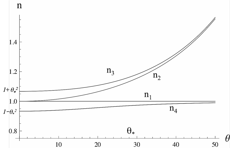
Figure 1: Dependence of the refractive indexes $n$ on angle $\theta$ for $A_{\rm p}\gg 1$. The lower branch corresponds to the O-mode

2.2 Kravtsov-Orlov equation

The Kravtsov-Orlov equation describes the evolution of the complex angle $\Theta=\Theta_{1}+i\Theta_{2}$, where $\Theta_{1}$ is a position angle of the polarization ellipse, and $\Theta_{2}$ determines the circular polarization by the relation $V=I\,{\rm tanh}2\Theta_{2}$. Here $I$ is the intensity of the wave, and $V$ is the Stokes parameter. As was shown (Andrianov & Beskin, 2010, Beskin & Philippov, 2011), the Kravtsov-Orlov equation can be rewritten as

$$\frac{{\rm d}\Theta_{1}}{{\rm d}l}= \frac{\omega}{2c}{\rm Im}[\varepsilon_{x^{\prime}y^{\prime}}]$$ (4)

$$-\frac{1}{2}\frac{\omega}{c}\Lambda\mathrm{cos}[2\Theta_{1}-2\beta(l)-2\delta(l)]{\rm sinh}2\Theta_{2},$$

$$\frac{{\rm d}\Theta_{2}}{{\rm d}l}= \frac{1}{2}\frac{\omega}{c}\Lambda\sin[2\Theta_{1}-2\beta(l)-2\delta(l)]{\rm cosh}2\Theta_{2},$$ (5)

where

$$\Lambda=\mp\sqrt{({\rm Re}[\varepsilon_{x^{\prime}y^{\prime}}])^{2}+\left(\frac{\varepsilon_{x^{\prime}x^{\prime}}-\varepsilon_{y^{\prime}y^{\prime}}}{2}\right)^{2}},$$ (6)

where the signs corresponds to the regions before/after the cyclotron resonance and

$$\tan(2\delta)=-\frac{2{\rm Re}[\varepsilon_{x^{\prime}y^{\prime}}]}{\varepsilon_{y^{\prime}y^{\prime}}-\varepsilon_{x^{\prime}x^{\prime}}}.$$ (7)

We would like to note, that in this equations the circular polarization is defined as it is common in radioastronomy (positive V corresponds to the co - clockwise rotating electric field vector for the observer). Here $l$ is a coordinate along the ray propagation, and the angle $\beta(l)$ defines the orientation of the external magnetic field in the picture plane. In the geometric optics region ($r<r_{\rm esc}$) the O-mode corresponds to polarization $\Theta_{1}\approx\beta+\delta$, and X-mode corresponds to $\Theta_{1}\approx\beta+\delta+\pi/2$.

Finally, $\varepsilon_{i^{\prime}j^{\prime}}$ are the components of plasma dielectric tensor in the reference frame where $z$-axis directs along the wave propagation and the external magnetic field lies in $xz$-plane. In comparison with model considered by Andrianov & Beskin (2010), equations (4)–(5) include into consideration nonzero components ${\rm Re}[\varepsilon_{x^{\prime}y^{\prime}}]$. It allows us to take into account the electric drift of plasma particles. This effect just corresponds to aberration considered by Blaskiewicz, Cordes & Wasserman (1991). This effect was also considered by Petrova & Lyubarskii (2000a), but for the infinite magnetic field only.

Thus, knowing the magnetic field structure and plasma properties of the outgoing plasma (i.e., knowing the dielectric tensor $\varepsilon_{i^{\prime}j^{\prime}}$) one can determine the observable physical quantities, namely, the Stokes parameter $V=I{\rm tanh}2\Theta_{2}(\infty)$ defining the CP and the position angle $p.a.=\Theta_{1}(\infty)$ characterizing the orientation of the polarization ellipse. This approach is valid in the quasi-isotropic case when there are two small parameters, i.e., the general WKB condition $1/kL\ll 1$ and the condition $\Delta n/n_{1,4}\ll 1$, where $\Delta n=n_{1}-n_{4}$.

2.3 Main predictions of the propagation theory

As the refractive index $n_{4}$ differs from unity, the appropriate ordinary mode is to deflect from the magnetic axis until $\theta\leq\theta_{*}$. As was already mentioned, for the O-mode this effect takes place until $A_{\rm p}>1$, i.e., for small enough distances from the neutron star $r<r_{\rm A}$, where

$$r_{\rm A}\approx 10^{2}R\,\lambda_{4}^{1/3}\,\gamma_{100}^{1/3}\,B_{12}^{1/3}\,\nu_{\rm GHz}^{-2/3}\,P^{-1/3}.$$ (8)

Here $R$, $P$, and $B_{12}$ are the netron star radius, rotation period (in s), and magnetic field (in $10^{12}$ G), respectively. Accordingly, $\gamma_{100}=\gamma/100$, $\nu_{\rm GHz}$ is the wave frequency in GHz, and $\lambda_{4}=\lambda/10^{4}$, where $\lambda=n_{\rm e}/n_{\rm GJ}$ is the multiplicity of the particle creation near magnetic poles ($n_{\rm GJ}=\Omega B/2\pi ce$ is the Goldreich-Julian concentration). On the other hand, the transverse extraordinary wave with the refractive index $n=1$ (X-mode) is to propagate freely. As the radius $r_{\rm A}$ is much smaller than the escape radius $r_{\rm esc}$ (Cheng & Ruderman, 1979, Andrianov & Beskin, 2010)

$$r_{\rm esc}\approx 10^{3}R\,\lambda_{4}^{2/5}\,\gamma_{100}^{-6/5}\,B_{12}^{2/5}\,\nu_{\rm GHz}^{-2/5}\,P^{-1/5},$$ (9)

one can consider the effects of refraction and limiting polarization separately. In particular, this implies that one can consider the propagation of waves in the region $r\sim r_{\rm esc}$ as rectilinear.

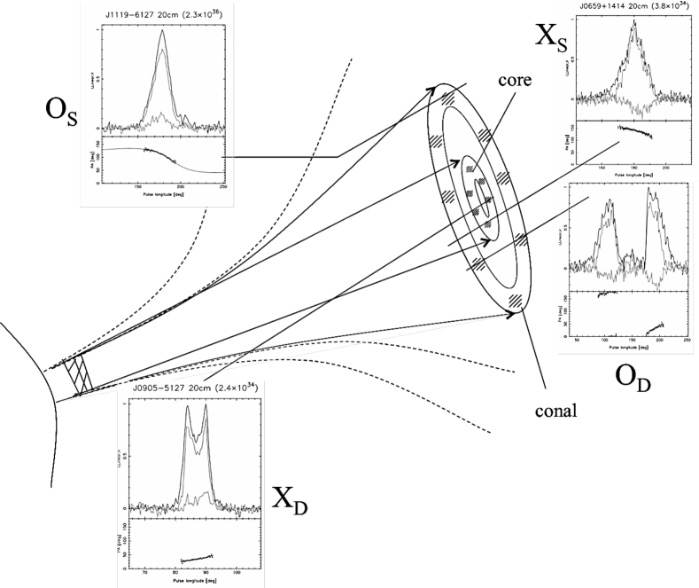
Figure 2: Propagation of X- and O-modes in the pulsar magnetosphere. The lower curve on each top panel of each picture indicates V, on the bottom panel p.a. curve is shown.

As a result, as shown in Fig. 2, if two modes are generated at the same distance $r_{\rm gen}<r_{\rm A}$ from the neutron star where $A_{\rm p}(r_{\rm gen})>1$, the directivity pattern of the O-mode is to be wider than that for the X-mode. Hence, it is logical to assosiate the X-mode with the core component of the directivity pattern. On the other hand, the O-mode is to form the conal component. E.g., assuming the constant plasma density across the flow (more realistic regime was considered by Petrova & Lyubarskii, 2000), Beskin, Gurevich & Istomin (1993) obtained for the radio window width $W_{\rm r}$

$$W_{\rm r}^{({\rm X})} \approx 3.6^{\circ}\,P^{-3/4}\,\nu_{\rm GHz}^{-1/2},$$ (10)

$$W_{\rm r}^{({\rm O})} \approx 7.8^{\circ}\,P^{-0.43}\,\nu_{\rm GHz}^{-0.14},$$ (11)

$$W_{\rm r}^{({\rm O})} \approx 10^{\circ}\,P^{-0.5}\,\nu_{\rm GHz}^{-0.29}.$$ (12)

For the O-mode, the theory gives two radiation beam widths, depending on the distribution of the energy release power in height.

The main new theoretical result based on the analysis of Kravtsov-Orlov equations (4)–(5) is that for large enough derivative ${\rm d}(\beta+\delta)/{\rm d}l$, the sign of the Stokes parameter $V$ is to be determined not by the poorly defined nondiagonal components of the dielectric tensor $\varepsilon_{x^{\prime}y^{\prime}}$, when $V_{0}/I=\pm 1/q$ (Zheleznyakov, 1977) and

$$q=i\,\frac{\varepsilon_{y^{\prime}y^{\prime}}-\varepsilon_{x^{\prime}x^{\prime}}}{2\varepsilon_{x^{\prime}y^{\prime}}},$$ (13)

but by the sign of the derivative ${\rm d}(\beta+\delta)/{\rm d}l$. It takes place when one can neglect the first term in the r.h.s. of Eqn. (4) in comparison with the derivative ${\rm d}\Theta_{1}/{\rm d}l\approx{\rm d}(\beta+\delta)/{\rm d}l$. E.g., for $r\ll r_{\rm esc}$ ($|V|\ll 1$):

$$\frac{V}{I}\approx\frac{1}{|q|}\cdot\frac{{\rm d}(\beta+\delta)/{\rm d}x}{|v_{\parallel}/c-\mathrm{cos}\theta|}\,\frac{1}{\mathrm{cos}[2\Theta_{1}-2\beta(l)-2\delta(l)]}.$$ (14)

Here $x=\Omega l/c$ is dimensionles distance along the ray.

Hence, for large enough ${\rm d}(\beta+\delta)/{\rm d}x\sim 1$ (the total turn $\Delta(\beta+\delta)\sim 1$ within the light cylinder $R_{\rm L}=c/\Omega$), and for small angle of propagation $\theta\ll 1$ through the relativistic plasma ($v_{\parallel}/c\sim 1$) the Stokes parameter $V$ (14) is indeed much larger than $V_{0}/I=\pm 1/q$ resulting from standard evaluation. Moreover, numerical calculations (Beskin & Philippov, 2011) shows that the sign of the derivative ${\rm d}(\beta+\delta)/{\rm d}l$ is opposite to the sign of the derivative ${\rm d}p.a./{\rm d}\phi$.

As a result, one can formulate the following predictions:

• For the X-mode ($\Theta_{1}\approx\beta+\delta+\pi/2$) the theory predicts the SAME signs of the circular polarization $V$ and the derivative ${\rm d}p.a./{\rm d}\phi$.

• For the O-mode ($\Theta_{1}\approx\beta+\delta$) the signs of the circular polarization $V$ and the derivative ${\rm d}p.a./{\rm d}\phi$ are to be OPPOSITE.

• For radio pulsar with the tripple mean pulses we have to see the O-mode first, than X- and again the O-mode because, as was shown in Fig. 2, the O-mode deviates from magnetic axis.

• In general, the trailing part of the main pulse can be absorbed (see Dyks, Wright & Demorest, 2010 as well).

• The leading component can be absorbed only if the polarization formes near the light cylinder ($r_{\rm esc}\sim R_{\rm L}$). In this case the $p.a.$ is to be approximately constant in given mode as the magnetic field here is approx. homogeneous (A.Spitkovsky, private communication).

• Statistically, we expect single profiles for the X-mode (if only the X-mode is observed) and the double ones for the O-mode.

In the following section we will try to demonstrate that these predictions are indeed in good agreement with observational data.

3 Comparison with observations

3.1 Statistics on single-mode pulsars

In Table 1 we collected more than 70 pulsars from two reviews by Weltevrede & Johnston (2008) and Hankins & Rankin (2010) for which both the values of $p.a.$ and $V$ were well-determined. As was predicted, most pulsars with double (D) mean profile corresponds to the O-mode (the opposite signs of $V$ and ${\rm d}p.a./{\rm d}\phi$), and the most pulsars with single (S) mean profiles – to the X-mode (the same signs of $V$ and ${\rm d}p.a./{\rm d}\phi$). Moreover, statistically the O-mode pulsars have wider mean pulses than X-mode, their values being in good agreement with theoretical predictions (10)–(12).

Table 1: Statistics of pulsars with known circular polarization $V$ and position angle swing. Pulsar period $P$ is in seconds, and the window width $W_{50}$ is in degrees.

${\rm Profile}$	${\rm O_{S}}$	${\rm O_{D}}$	${\rm X_{S}}$	${\rm X_{D}}$
Number	6	23	45	6
$\sqrt{P}W_{50}$	6.8$\pm$ 3.1	10.7$\pm$ 4.5	6.5$\pm$ 2.9	5.3$\pm$ 3.0

3.2 Pulsars with almost constant $p.a.$

In Table 2 we collected ten pulsars with almost constant $p.a.$ from the papers by Johnston et al. (2007) ([1] in the reference column), Mitra and Rankin (2010) ([2]), and Johnston et al. (2008) ([3]). One can note that their rotational periods are smaller than 1 s, i.e., the typical pulsar period. Also four of them (indicated by plus in the comment column) show the ”flatting” of the $p.a.$ swing with the frequency decreasing. The interpretation of these effects can be easily given basing on the estimate of the escape radius $r_{\rm esc}$ (9), where the polarization of the radio emission forms (Andrianov & Beskin, 2010). As $r_{\rm esc}/R_{\rm L}\propto P^{-6/5}\nu^{-2/5}$, one can see that for small pulsar periods and lower frequencies the outgoing polarization forms closer to the light cylinder where magnetic field of neutron star, as was already stressed, is almost homogeneous. In this case the $p.a$ of the outgoing radiation is to be approximately constant within the mean pulse. This effect was firstly introduced by Barnard (1986), the main distinction of our theory is in self-consistent definition of $r_{\rm esc}$ basing on the solution of equations (4)–(5).

Table 2: Pulsars with almost constant p.a. Here P is in seconds, $\dot{P}$ is in $10^{-15}$, and magnetic field $B$ on the surface of neutron star is in $10^{12}$ G

${\rm PSR}$	$P(s)$	$\dot{P}$	$B_{12}$	comment	reference
J0543$+$2329	0.25	15.4	2.0	+	[3]
J0738$-$4042	0.37	1.6	0.8	+	[1]
J0837$-$4135	0.75	3.5	1.6		[1]
J1559$-$4438	0.26	1.0	0.5	+	[3]
J1735$-$0724	0.42	1.2	0.7		[1]
B1907$-$03	0.50	2.2	1.0		[2]
J1915$+$1009	0.40	1.5	2.5		[1]
J1937$+$2544	0.20	0.6	0.4	+	[1]

3.3 Pulsars with tripple mean profiles

Below we analyse the profiles of several tripple pulsars presented in review by Johnston et al. (2007) for which both $p.a.$ and $V$ are well-determined at any way at one frequency, 693, 1374, or 3100 MHz.

For pulsar PSR J0452$-$1759 the triple structure is seen at 693 MHz only. For this reason, it is not surprizing that the $90^{\circ}$-switch of the $p.a.$ from O-mode to X-mode and return is seen on this frequency only. The CP is well-determined in the trailing subpulse only, where its sign, as was predicted, corresponds to O-mode.

The tripple structure of the pulsar PSR J0738$-$4042 is seen on the $p.a.$ profile at 691 MHz only. Nevertheless, as the $p.a.$ is approximately constant at low frequency (see Table 2), one can assume that the leading part of the profile is absorbed. Then, the leading subpulse is to correspond the X-mode, and the trailing one – to the O-mode (the appropriate negative CP is seen in this subpulse only).

In pulsar PSR J1559$-$4438 the tripple structure O-X-O is well-seen at all frequencies 691, 1374, and 3100 MHz, but in the mean profile the conal component is detected at the frequency 3100 MHz only. The negative CP for core subpule corresponding to the X-mode is seen at all frequencies.

The CP of the tripple pulsar PSR J2048$-$1616, as was predicted, corresponds to O-X-O structure. On the other hand, the switch of the $p.a.$ is absent, that can be caused, in our opinion, by the averaging technique and should be checked in the individual profiles as well (one can see the influence of the averaging technique on the CP profile in Karastergiou et al., 2003).

Thus, as we see, the properties of the pulsars with triple mean profiles are in good agreement with the theoretical predictions. The central (core) components of the mean profiles, in general, connect with the X-mode propagating freely, while the conal parts correspond to the O-mode deflecting via the refraction from the magnetic axis.

3.4 Pulsars with interpulses

Here the same analysis for pulsars with interpulses from paper by Keith et al. (2010) is given. The observations were made at the frequency 1.4 GHz.

The main pulse of pulsar PSR J0627$+$0706 is to be connected with the O-mode (it has the opposite signs of $p.a.$ and $V$). The trailing subpulse of the double profile, as is well seen from the $p.a.$ swing (the observable subpulse corresponds to the first half of the S-shape curve) is absorbed. In the interpulse the circular polarization is not high enough to determine modes.

The central part of the main pulse of pulsar PSR J1549$-$4848 is formed by the X-mode (the same signs of the $p.a.$ and $V$). In the leading and the trailing parts of the main pulse the CP is too low to say anything about the conal component. The interpulse has the triple structiure, the sequence of the modes, as was predicted, being O-X-O. This is clear not only from the negative-positive-negative sequence of the Stokes parameter $V$ but from the singularity of the $p.a.$ at the phase $\phi=-85^{\circ}$.

The main pulse of pulsar PSR J1722$-$371 is formed mainly by the X-mode. The CP of the interpulse is too low to determine the modes.

The double main pulse of the pulsar PSR J1739$-$2903 is to be interpreted as the sequence of the O- and X-modes. It is clear both from the negative-to-positive change of the Stokes parameter $V$ and from the $90^{\circ}$ jump in $p.a.$ The trailing (O-mode) component is absorbed because, as for PSR J0627$+$0706, the leading O-mode subpulse corresponds only to the first half of the S-shape curve of the $p.a.$. The interpulse is formed by the X-mode.

In the main pulse of pulsar PSR J1828$-$1101 the value $V$ is not high enough to determine the mode. The interpulse is formed mainly by the O-mode, the trailing subpulse being absorbed (here again the $p.a.$ of the visible pulse corresponds to the first half of the S-shape curve).

Thus, for radio pulsars with interpulse the interpretation on the ground of the theory under consideration is reasonable as well.

3.5 Milliseconds pulsars

Finally, we consider the millisecond pulsars which detailed polarization characteristics were presented recently by Yan et al., (2011). The observations were made at the frequency 1369 MHz.

Pulsar PSR J0437$-$4715 has the multiple mean profile. Its leading and the trailing parts (i.e., the conal component) definitely corresponds to the O-mode. On the other hand, both the $90^{\circ}$ jump in $p.a.$ and the change of the Stokes parameter sign in the core component shows that the central subpulse consists not only of the X-mode, but of the O-mode as well.

The leading and the trailing components of the double profile of pulsar PSR J1022$+$1001, in agreement with the prediction, are formed by the O-mode. The peak on the $p.a.$ curve in the center of the mean profile could be connected with the core X-mode, but its intensity is too low to be seen on the mean pfofile.

Pulsar PSR J1045$-$4509 has the triple main profile. It has different signs of the circular polarization in the core and conal components. But the position angle swing is irregular, which prevent us to determine the modes.

In pulsar PSR J1600$-$3053 the core component is definitely formed by the X-mode (the same signs of the Stokes parameter $V$ and the derivative ${\rm d}p.a./{\rm d}\phi$). Then, the conal component is to be connected with the O-mode as its $p.a.$ curve locates approx. $90^{\circ}$ higher that that for the core component. The circular polarization is too low to confirm this point.

The circular polarization of the central part of the double profile of pulsar PSR J1603$-$7202 is different from the conal ones. The irregular character of the $p.a.$ swing does not allow us to determine the mode.

Pulsar PSR J1643$-$1224 has the single main profile which can be easily interpreted as standard O-X-O sequence with the absorbed trailing part. Indeed, the polarization of the leading part definitely corresponds to the O-mode (the different signs of $V$ and ${\rm d}p.a./{\rm d}\phi$), while the trailing part is to be connected with the X-mode (the same signs of $V$ and ${\rm d}p.a./{\rm d}\phi$). Moreover, the derivative ${\rm d}p.a./{\rm d}\phi$ is much larger in the trailing part. This implies that the visible pulse corresponds the first half of the S-shape curve.

Pulsar PSR J1713$+$0747 has multicomponent profile containing both modes. It has different signs of the circular polarization for different branches of the p.a. curves.

Pulsar PSR J1732$-$5049 has actually zero circular polarization which does not allow us to determine the modes. Nevertheless, one can see that the $p.a.$ of the core and conal parts belongs to the different modes.

The profile of pulsar PSR J1909$-$3744 is quite similar to PSR J1643$-$1224. Hence, it can be easily interpreted as O-X-O sequence with the absorbed trailing part as well.

Radiation of pulsar PSR J2129$-$5721 is to be connected with the core conponent formed by the X-mode (the same signs of $V$ and ${\rm d}p.a./{\rm d}\phi$). Two subpulses of the mean profile can be easily explained by the central passage through the directivety pattern (see Fig. 2).

In addition, the double profile pulsars PSR J0613$-$0200, J0711$-$6830 have the same signs of the Stokes parameter $V$ in both subpulses. But it is impossibe to connect them with the O-mode because of the irregular swing ofthe $p.a.$. Finally, pulsars J1024$-$0719, J1730$-$2304, J1744$-$1134, J1824$-$2452, J1857$+$0943, 2124$-$3358, and J2145$-$0750 have irregular structure or actually zero circular polarization which does not allow us to analyse their properties.

Thus, in that cases when the $p.a.$ swing and the Stokes parameter $V$ are regular enough, the main properties of the mean profiles can be easily interpreted within the theory under consideration.

4 Acknowledgments

We thank A.V. Gurevich and Y.N. Istomin for their interest and support, J. Dyks, A. Jessner, D. Mitra, M.V. Popov, B. Rudak and H.-G. Wang for useful discussions, and an anonymous referee for valuable suggestions that greatly improved the quality of this article. This work was partially supported by Russian Foundation for Basic Research (Grant no. 11-02-01021).

References

- Andrianov & Beskin (2010) Andrianov A.S., Beskin V.S., 2010, Astron. Letters, 36, 248
- Barnard (1986) Barnard J.J., 1986, ApJ, 303, 280
- Barnard & Arons (1986) Barnard J.J., Arons J., 1986, ApJ, 302, 138
- Beskin & Philippov (2011) Beskin V.S., Philippov A.A., 2011 (in preparation)
- Beskin & Gurevich & Istomin (1993) Beskin V.S., Gurevich A.V., Istomin Y.N., 1993, Physics of the Pulsar Magnetosphere, Cambridge University Press, Cambridge
- Blaskiewicz, Cordes & Wasserman (1991) Blaskiewicz M., Cordes J.M., & Wasserman I., 1991, ApJ, 370, 643
- Cheng & Ruderman (1979) Cheng A.F., Ruderman M.A., 1979, ApJ, 229, 348
- Dyks, Wright & Demorest (2010) Dyks J., Wright G.A.E., Demorest P.B., 2010, MNRAS, 405, 509
- Hankins & Rankin (2010) Hankins T.H., Rankin J.M., 2010, AJ, 139, 168
- Johnston & Kramer (2005) Johnston S., Karastergiou A., Mitra D., Gupta Y., 2008, MNRAS, 388, 261
- Johnston & Kramer (2007) Johnston S., Kramer M., Karastergiou A., Hobbs G., Ord S., Wallman J., 2007, MNRAS, 381, 1625
- Karast (2003) Karastergiou A., Johnston S., Kramer M., 2003, A&A, 404, 325
- Johnston & Kramer (2010) Keith M.J., Johnston S., Weltrvrede P., Kramer M., 2010, MNRAS, 402, 745
- Kravtsov & Orlov (1990) Kravtsov Yu.A., Orlov Yu.I., 1990, Geometrical Optics of Inhomogeneous Media, Springer, Berlin
- Melrose & Gedalin (1999) Melrose D.B., Gedalin M.E., 1999, ApJ, 521, 351
- Mitra & Rankin (2010) Mitra D., Rankin J.M., 2010, ApJ, 727, 92
- Petrova (2001) Petrova S.A., 2003, A&A, 408, 1057
- Petrova (2006) Petrova S.A., 2006, MNRAS, 368, 1764
- Petrova & Lyubarskii (2000a) Petrova S.A., Lyubarskii Yu.E., 2000, A&A, 355, 1168
- Wang & Lai &Han (2010) Wang C., Lai D., Han J., 2010, MNRAS, 403, 2
- Weltvrede & Johnston (2008) Weltrvrede P., Johnston S., 2008, MNRAS, 391, 1210
- Yan et al (2011) Yan W.M., Manchester R.N., van Straten W. et al., 2011, arXiv:1102.2274
- Zheleznyakov (1964) Zheleznyakov V.V., 1970, Radio Emission of the Sun and Planets, Pergamon, Oxford
- Zheleznyakov (1977) Zheleznyakov V.V., 1996, Radiation in Astrophysical Plasmas, Springer, Berlin