Finite temperature study of bosons in a two dimensional optical lattice

Abstract

We use quantum Monte Carlo (QMC) simulations to study the combined effects of harmonic confinement and temperature for bosons in a two dimensional optical lattice. The scale invariant, finite temperature, state diagram is presented for the Bose-Hubbard model in terms of experimental parameters – the particle number, confining potential and interaction strength. To distinguish the nature of the spatially separated superfluid, Mott Insulator and normal Bose liquid phases, we examine the local density, compressibility, superfluid density and Green’s function. In the annular superfluid rings, as the width of the ring decreases, the long range superfluid correlations start to deviate from an equivalent homogeneous 2D system. At zero temperature, the correlation decay is intermediate between 1D and 2D, while at finite temperature, the decay is similar to that in 1D at a much lower temperature. The calculations reveal shortcomings of the local density approximation (LDA) in describing superfluid properties of trapped bosons. We also present the finite temperature phase diagram for the homogeneous two dimensional Bose-Hubbard model. We compare our state diagram with the results of a recent experiment at NIST on a harmonically trapped 2D lattice [Phys. Rev. Lett. 105, 110401 (2010)], and identify a finite temperature effect in the experiment.

I Introduction

Much progress has been made in the last decade in the use of trapped, ultracold atoms for the optical lattice emulation of tight binding Hamiltonians greiner02 ; jaksch98 ; lewenstein07 ; bloch08 . In the bosonic case, Quantum Monte Carlo (QMC) simulations are possible on very large lattices (algorithms scale linearly with the system size) and at low temperatures (no sign problem). As a result, close contact between experiments and theory has been possible, with successful quantitative comparisons of momentum distributions and phase transition critical points spielman10 ; spielman0708 ; trotzky09 . Recent QMC simulations of the homogeneous system have refined early determinations batrouni90 ; trivedi91 ; freericks96 of the critical point for the ground state superfluid-Mott insulator boundary to very high accuracy sansone08 , and have also examined the finite temperature behavior at integer filling sansone08 . QMC studies which include a confining potential and hence determine a “state diagram” showing which phases coexist as a function of interaction strength and characteristic density have also been reported at low temperature rigol09 and compared to experiment spielman10 ; spielman0708 .

In current experiments, spielman10 ; spielman0708 ; trotzky09 ; cchin09 ; cchin10 ; bakr09 ; sherson10 ultracold atoms are first loaded in a harmonic trap, and then an external sinusoidal potential is slowly ramped up to create the optical lattice. By varying the depth of the lattice, the interaction strength ($U/t$) is changed, thereby driving the system through a quantum phase transition from a superfluid (SF) phase to a Mott insulating (MI) phase. Although the initial system can be prepared at a relatively low temperature, the ensuing system after ramp-up of the lattice has a temperature which is usually higher due to adiabatic and other heating mechanisms cchin10 ; pupillo06 ; pollet08 ; ho07 ; mahmud10 . Recent experiments have reported temperatures on the order of $T/t\approx 0.9/k_{B}$ spielman10 . At such temperatures, the effects of excited states become important, motivating investigations into the finite temperature phase diagram, quantum versus thermal transitions, the location of spatially separated phases in a trap at finite-T, etc. Aspects of finite-T effects on the MI have been discussed in Ref. sansone08 ; gerbier07 ; demarco07 . Several QMC studies have also appeared at zero and finite temperatures, dealing with quantum criticality and phase coexistence in a trap wessel04 ; zhou09 ; kato08 ; roscilde10 ; pollet10 ; fang10 ; hazzard10 ; ma10 .

The goal in this paper is to provide a study of the combined effects of a confining potential and finite temperature on the state diagram of the Bose-Hubbard model in two dimensions, generalizing previous finite-T QMC work sansone08 at fixed density, and ground state QMC studies in the presence of a confining potential batrouni02 ; rigol09 . In addition to the trapped state diagram, we present the finite temperature phase diagram of the homogeneous 2D Bose-Hubbard model. Our results quantify the spatial inhomogeneity/phase coexistence which is created by the trap and the interplay of thermal fluctuations, which give rise to a third, normal (N) liquid phase in addition to the usual ground state SF and MI phases of the Bose Hubbard model fisher89 . We use an appropriately scaled measure of particle number, the ‘characteristic density’, which allows systems of different sizes to be compared rigol09 , to present the scale invariant finite temperature state diagram. We compare our state diagrams with the results of a recent NIST experiment on a harmonically trapped 2D lattice spielman10 , and identify a finite temperature effect in the experimental data. To better understand the nature of the trapped phases, we investigate the correlation function decay. In the annular superfluid rings, the correlation decay is different from an equivalent homogeneous 2D superfluid – matching for a short distance and then falling off at a faster rate for longer distances. At zero temperature, the correlation decay is intermediate between 1D and 2D, while at finite temperature, the decay is similar to 1D at a much lower temperature. In short, the width of the trap and the temperature determine the 2D to 1D crossover. These findings provide evidence for the breakdown of the local density approximation (LDA) for the description of superfluid properties of trapped bosons.

The article is organized as follows. In Sec. II, the Bose-Hubbard model fisher89 and the observables used to monitor the state diagram are introduced. The QMC methodology is also briefly described. In Sec. III, we present the QMC homogeneous system phase diagram at finite-T. In Sec. IV, we analyze finite temperature effects in a harmonically trapped system, present the state diagram at zero and finite temperature, and compare them with a recent NIST experiment spielman10 . In Sec. V, we examine the dependence of spatial correlations in the trapped superfluid rings, and present evidence for the breakdown of LDA. Finally, we summarize our results in Sec. VI.

II Model and computational methods

Cold bosonic atoms in the lowest band of an optical lattice can be modeled by the Bose-Hubbard model,

$$H = -t\sum_{\langle i,j\rangle}\left(a^{\dagger}_{i}a_{j}+a^{\dagger}_{j}a_{i}\right)+\dfrac{U}{2}\sum_{i}n_{i}\left(n_{i}-1\right)$$ (1)

$$+V_{T}\sum_{i}r_{i}^{2}\ n_{i}-\mu\sum_{i}n_{i}\,\,,$$

Here $a^{\dagger}_{i}$, $a_{i}$ are the creation and annihilation operators of a boson at site $i$, $n_{i}=a^{\dagger}_{i}a_{i}$ is the number of bosons, $t$ is the strength of hopping foot1 between nearest neighbors (here on a square lattice), and $U$ is the on-site repulsive interaction. $V_{T}$ is the curvature of the external harmonic trap which introduces inhomogeneity to the system. $r_{i}^{2}=x_{i}^{2}+y_{i}^{2}$ is the distance from the center of the trap, $x_{i}=d\times i$, where $d$ is the period of the lattice, and $i$ an integer. The hopping $t$, interaction $U$, and trap curvature $V_{T}$ are tunable parameters in the experiment.

In this paper we use the modified directed-loop algorithm kato0709 for the QMC simulation based on the Feynman path integral kawashima04 , since the simple application of directed-loop algorithm to the Bose-Hubbard model, that has the widest applicability, is not efficient especially for large $U/t$.

To obtain the phase diagram, we examine three local observables – the density $\rho_{i}=\langle\,n_{i}\,\rangle$, compressibility $\kappa_{i}$, superfluid density $\rho_{s}$, and Green’s function $g(i,j)$. Together, these variables are able to distinguish the spatially separated phases in a trap. The local compressibility is a measure of the response of the local density to a change in the chemical potential,

$$\kappa_{i}=\frac{\partial\langle n_{i}\rangle}{\partial\mu_{i}}=\int_{0}^{\beta}d\tau[\langle n_{i}(\tau)n_{i}(0)\rangle-\langle n_{i}(\tau)\rangle\langle n_{i}(0)\rangle]$$ (2)

Here $\mu_{i}=\mu-V_{T}r_{i}^{2}$ is the site dependent local chemical potential which decreases away from the trap center, and $\beta=1/T$ is the inverse temperature. For a trapped system, a qualitative criterion for the appearance of a local MI is that the local density be an integer, as for the homogeneous case. At $T=0$, a more precise criterion for identifying a local MI is to require that $\kappa_{i}$ take on a value equal to the compressibility, $\kappa=\partial\rho/\partial\mu$, of a homogeneous system of commensurate filling batrouni02 ; rigol09 . It is typically the case that an extended (more than 4-5 sites) region of nearly constant, integer density has $\kappa_{i}$ close to its value in the homogeneous MI, thus providing a more rapid, visual means to identify a likely MI region. For finite-T, since the MI-N boundary is a crossover, there is no sharply defined phase boundary, and there is arbitrariness in drawing such a boundary. In delineating the crossover boundary for the homogeneous and the trapped system at finite temperature, we have taken $\kappa<0.02/U$ to identify the Mott region. A superfluid region has a nonzero superfluid density, while the normal region is identified as the region with zero superfluid density and incommensurate filling with $\kappa>0.02/U$.

The Green’s function, or one-particle density matrix,

$$g(i,j)=\langle a^{\dagger}_{i}a_{j}\rangle$$ (3)

is useful in identifying SF regions. Specifically, a $g(i,j)$ which falls off sufficiently slowly as $|i-j|$ becomes large signals the development of off-diagonal long range order. Conversely, a rapid (exponential) fall-off of $g(i,j)$ is consistent with the appearance of a N or MI phase.

To define a local SF density is more subtle, since $\rho_{s}$ involves the response of the system to a global phase twist. While there may be a way to generalize this to a local quantity, here we adopt the simpler LDA approach, assigning the homogeneous system value of $\rho_{s}$ to different spatial locations of the confined system zhou09 . This gives an initial state diagram for confined systems. The correlation function $g(i,j)$ provides more information about the superfluid properties of the finite width annular superfluid rings.

III Homogeneous Systems at Finite Temperature

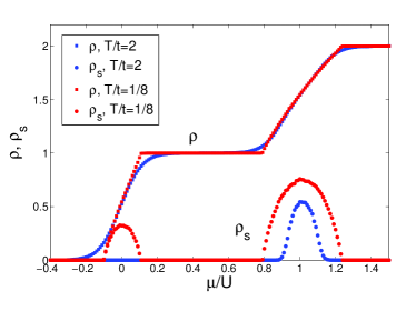
Figure 1: (color online). Occupation ($\rho$) and SF density ($\rho_{s}$) as a function of the chemical potential ($\mu/U$) for two different temperatures $T/t=2$ and $T/t=1/8$ at $t/U=0.025$ for the homogeneous 2D Bose-Hubbard model calculated using QMC simulations on a $32\times 32$ lattice. A nonzero $\rho_{s}$ corresponds to a superfluid (SF) phase, zero $\rho_{s}$ with integer occupation $\rho=1$ and vanishing compressibility to a Mott insulator (MI) phase, and zero $\rho_{s}$ with non-integer occupation to a normal (N) phase. The key point is that at the low temperature, wherever the density is incommensurate, the system is also SF. There are only MI and SF regions, and no N liquid. On the other hand, at higher temperature, normal regions develop which have incommensurate filling but also $\rho_{s}=0$. This is made clear in the figure at the incommensurate density region near $\mu/U=0$ where a rise in temperature from $T/t=1/8$ to $T/t=2$ has destroyed the superfluid density turning the SF to N. Looking at the $\rho_{s}$ values, it is also evident that the superfluid properties at higher occupation ($1<\rho<2$) such as around $\mu/U=1$ is stronger than that of the low occupation ($0<\rho<1$) around $\mu/U=0$.

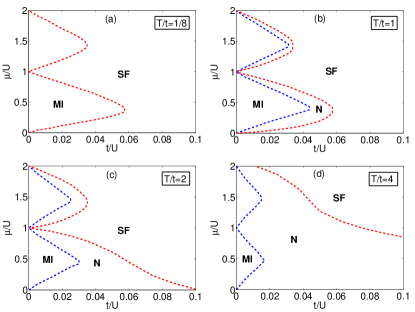
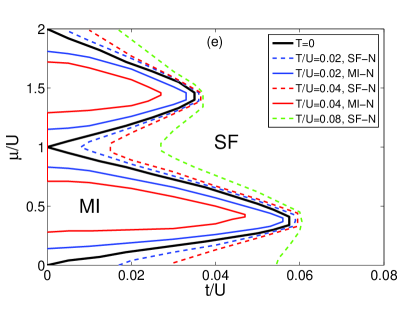
Figure 2: (color online). Finite temperature phase diagram for the homogeneous Bose-Hubbard model in two dimensions in the ($\mu/U,t/U$) plane for four different temperatures (a) $T/t=1/8$, (b) $T/t=1$, (c) $T/t=2$ and (d) $T/t=4$. (e) shows the phase diagram in a different representation, for constant $T/U$ values of 0.02, 0.04 and 0.08. The lines that demarcate the SF and N is a phase boundary, and the lines that demarcate MI and N is a crossover. At finite temperature, normal phase regions appear between MI and SF. These normal regions grow bigger for higher temperature. Although the finite-T homogeneous phase diagram is usually presented as in panel (e), with $T$ in units of $U$, the phase diagram plots (a)-(d) for constant $T/t$ values connect well to the confined system state diagram presented in Sec. IV, and provide a useful representation for optical lattice experiments.

The zero temperature ground state phase diagram for the homogeneous Bose-Hubbard model ($V_{T}=0$) in two dimensions has been worked out using strong coupling expansions freericks96 , and most recently using QMC sansone08 . In Ref. sansone08, , a finite temperature phase diagram for a constant occupation $\rho=1$ was presented showing the boundaries of the SF and MI/N regions in the ($T/t,U/t$) plane. Mean-field theory has been used sheshadri93 ; lu06 ; bounsante04 to study different properties and to obtain the finite-T phase diagram in any dimension. Various other approximate methods have also been used to study the finite temperature Bose-Hubbard model polak09 ; ohliger08 . We present here the QMC homogeneous finite-T phase diagram in the ($\mu/U,t/U$) plane valid for the first two commensurate filling lobes.

In Fig. 1 the density $\rho$ and the SF density $\rho_{s}$ are shown as functions of $\mu/U$ for two different temperatures $T/t=1/8$ and $T/t=2$ for a $32\times 32$ lattice at $t/U=0.025$. (This lattice size is large enough so that finite size effects are minor.) For $T/t=1/8$, $\rho_{s}$ is non-zero whenever $\rho$ is incommensurate. At this low temperature the system is either a MI or a SF. On the other hand, for $T/t=2$, this is no longer the case. There are substantial regions where $\rho_{s}$ is zero even though $\rho$ is incommensurate, which signifies a N liquid. For a homogeneous system, the boundary between the MI and normal regions in the finite temperature phase diagram is a crossover, as opposed to being a true phase transition at the SF-N boundary. The MI phase strictly speaking exists only at $T=0$. However, Mott-like features can persist at a finite temperature with a small value of compressibility. As mentioned in Sec. II, in drawing this MI-N crossover boundary at finite-T, we have taken $\kappa<0.02/U$ to identify the Mott region.

The QMC homogeneous system phase diagram for the 2D Bose-Hubbard model at finite temperature can be built up by sets of runs such as shown in Fig. 1 for different $U/t$, and is presented in Fig. 2. We show the phase boundaries for four different temperatures in panels (a)-(d); $T/t=1/8$, which is a low enough temperature to be the zero temperature phase diagram, $T/t=1$, $T/t=2$ and $T/t=4$. At $T/t=1/8$ the system has only two phases – MI with an energy gap inside the lobe, and a gapless SF outside the lobe. The transition between them is driven by quantum fluctuations as $t/U$ is varied. The lowest value of $U/t$ for which the SF-MI transition can occur is $U/t\approx 16.74$ (i.e. $t/U\approx 0.059$) sansone08 , the location being at the tip of the first lobe. At a finite temperature, thermal fluctuations play a part, and MI lobes are reduced. For example, at $T/t=1$ in Fig. 2(b), we see that between the MI and SF phases, a region of normal phase has developed at the expense of reducing both the SF and MI regions. With further increase of temperature, the normal phase region widens. For $T/t=2$, the N-SF phase boundary around $\rho=1$ is no longer lobe-like: the SF region ceases to bend back inward to low $t/U$ at small density. With further increase of temperature to $T/t=4$, the SF between the first two MI lobes is also replaced by N liquid.

In Fig. 2(e) we present the finite-T phase diagram for temperatures in units of $U$, for $T/U=0.02,0.04$ and $0.08$. As temperature increases, the MI lobes shrink, and the N liquid phase region grows between the MI and SF region. For $T/U=0.08$ we find that the compressibility $\kappa>0.02/U$ near $t/U=0$, which is therefore no longer a MI in our criteria. The pictorial representations of how the MI lobes behave, although different in the two representations of $T/t$ and $T/U$, are interchangeable. For a constant $T/t$ phase diagram, as $t/U$ decreases to zero, $T/U$ also goes to zero, and the MI lobes in (a)-(d) for low $t/U$ slowly approaches $\mu/U=0,1$ and $2$, giving rise to a lobe that looks pointy. Although finite-T homogeneous phase diagram is usually presented at constant $T/U$ as in panel (e), phase diagram plots (a)-(d) for constant $T/t$ values connect well to the confined system state diagram presented in Sec. IV, and provide a useful representation for optical lattice experiments where temperatures are often cited spielman10 ; spielman0708 in units of $T/t$.

We conclude this section by noting that Fig. 2 can be reinterpreted as giving the local density and SF profiles in a confined system, assuming the validity of the LDA. That is, to each spatial site in a confined lattice are associated the density and SF density of a homogeneous system with the same local chemical potential. The resulting sequence of LDA phases which occurs in moving away from the trap center can most easily be understood by starting with the location $(\mu/U,t/U)$, where $\mu$ is the chemical potential at the trap center, on the homogeneous phase diagram of Fig. 2 and moving downwards, since decreasing $\mu/U$ corresponds to increasing $V_{T}\,r_{i}^{2}$ and thus moving outward from the trap center.

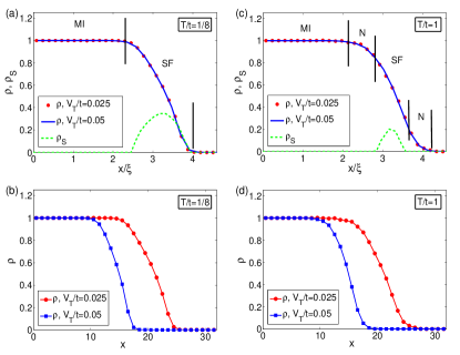
Figure 3: (color online). The validity of the characteristic density idea and the effects of temperature on spatially separated phases in a harmonically trapped system are illustrated. For $T/t=1/8$, panel (a) shows the density profiles for two systems with the same characteristic density $\tilde{\rho}=34.5$ but different trapping potentials and total number of particles, $V_{T}/t=0.025$, $N_{b}=1380$ and $V_{T}/t=0.05$, $N_{b}=690$. All position dependent quantities are equivalentrigol09 as a function of characteristic length scale $\xi=\sqrt{t/V_{T}}$, as evident here in density matching. (b) shows the actual density profiles for the two trapping strengths, highlighting how these two different spatial profiles match in the scaled plot (a). Density profiles in (a) exhibit a constant integer plateau and an incommensurate ring with $n<1$, calculated using QMC for a trapped system. (c) shows the density profile at a higher temperature, $T/t=1$, also showing a similar constant plateau and an incommensurate ring. To determine whether the ring contains a SF or N liquid, we plot LDA derived SF density across the trap which shows that for (a) the entire ring is SF, whereas in (c) only a portion of the ring is SF and the rest is N: $\rho$ is incommensurate but $\rho_{s}=0$. (d) shows the unscaled density profiles for the two trapping strengths in (c).

IV State diagram at finite temperature

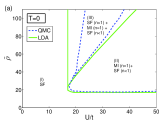
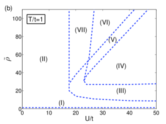
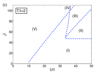
Figure 4: (color online). State diagrams for a harmonically trapped system for (a) $T=0$, (b) $T/t=1$ and (c) $T/t=2$. A schematic of all the phases according to their labels is shown in Fig. 5. The phase boundaries are drawn according to the multiple phases that coexist in a region. For example, in (a), region (II) corresponds to a state which has a MI plateau in the center surrounded by a SF shell. For higher T, normal (N) phase appears and therefore there are states with many varieties of coexisting phases. For example, phase (IV) in (b) has a MI in the center, surrounded outward by N, SF and N respectively. At a finite temperature, the tail always contains a normal liquid phase. For higher T, the SF-N phase boundary shifts to a lower value of $U/t$, and the first appearance of a MI plateau occurs at a higher value of $U/t$.

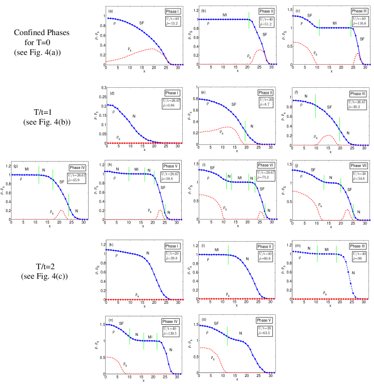
Figure 5: (color online). Schematic of all the phases for a trapped system at $T=0$, $T/t=1$, and $T/t=2$, according to the labels shown in the state diagrams in Fig. 4. At finite-T, part of the atomic cloud turns normal forming rings surrounding SF and MI regions, and three phases at $T=0$ increase to seven different phases at $T/t=1$ and five at $T/t=2$. The furthest part of the tail is always N at a finite-T as seen here in panels (d)–(o). Annular SF rings cannot form for a high enough temperature such as at $T/t=2$ shown in panels (k)–(o).

IV.1 Characteristic density

For the Bose-Hubbard model in the homogeneous case ($V_{T}=0$), the thermodynamic limit is reached by increasing the linear lattice size $L$ while keeping the density $\rho=N_{b}/L^{d}$ constant, where $N_{b}$ is the particle number, and $d$ is the dimensionality. The phase diagram is a function only of $U/t$, $T/t$ and $\rho$, not of $N_{b}$ and $L$ separately. In the same way, for the harmonically confined inhomogeneous system with $V_{T}\neq 0$, the generalization of this procedure rigol09 is to define a rescaled length, $\xi_{i}\equiv x_{i}/\xi$ with $\xi=\sqrt{t/V_{T}}$, and a ‘characteristic density’, $\tilde{\rho}=N_{b}/\xi^{d}$. For the 2D model, $\tilde{\rho}=N_{b}V_{T}/t$. The state diagram and the properties of the inhomogeneous system then depend only on the combination $\tilde{\rho}$. Measurements at fixed $U/t$, $T/t$ and $\tilde{\rho}$ then approach a well-defined large $L$ limit. Position dependent quantities match when plotted in units of rescaled length ($x_{i}/\xi$). Any LDA-derived quantities like $\rho$ or local $\rho_{s}$ trivially follow the rescaling.

The validity of characteristic density idea discussed in Ref. rigol09, is illustrated in Fig. 3. For $T/t=1/8$ (low enough to be effectively zero temperature), (a) shows the QMC density profiles for two systems with the same characteristic density $\tilde{\rho}=34.5$ but different trapping potentials and total number of particles, $V_{T}/t=0.025$, $N_{b}=1380$ and $V_{T}/t=0.05$, $N_{b}=690$. When plotted as a function of characteristic length scale $\xi=\sqrt{t/V_{T}}$, the density profiles are equivalent, as are all the position dependent local quantities rigol09 . (b) shows the actual density profiles for the two trap strengths in (a), clearly showing the different extent of the profiles and highlighting the concept of equivalence in the scaled plots in (a). The same holds true at finite-T, as shown in Figs. 3(c) and (d) for $T/t=1$. The density profile in (a) shows a constant integer plateau and an incommensurate ring with $n<1$, calculated using QMC for a trapped system. In panel (c) the density profile at a higher temperature, $T/t=1$, also shows a similar constant plateau and an incommensurate ring. To determine whether the ring contains a SF or N liquid phase, we plot LDA-derived SF density across the trap. This shows that for Fig. 3(a) the entire incommensurate ring is SF ($\rho_{s}\neq 0$), whereas in Fig. 3(c) only a small part of the ring is SF and the rest is N, where $\rho$ is incommensurate but $\rho_{s}=0$. This is how we identify trapped phases containing distinct combinations of MI, SF and N regions. Due to the validity of characteristic density scaling, the state diagram we obtain below is scale-invariant – not depending on the specific values of trap strength ($V_{T}$), number of particles ($N_{b}$) or lattice size, but on the combination $N_{b}V_{T}/t=\tilde{\rho}$. To obtain the state diagrams presented here, the largest lattice we used is $64\times 64$.

IV.2 Zero temperature state diagram

The state diagram for the harmonically confined system at zero temperature was presented in Ref. rigol09, . In Fig. 4(a), we show the $T=0$ state diagram in characteristic density – interaction strength ($\tilde{\rho}$, $U/t$) plane using QMC simulations in a trap, to higher values of $\tilde{\rho}$ than presented in Ref. rigol09, . Three separate states are possible here as indicated in Fig. 4(a), and illustrated in Fig. 5. The region (I) corresponds to SF phase all across the trap. In region (II), there is a MI plateau with ($n=1$) in the center, surrounded by a SF ring of $n<1$. (III) is a state (see Fig. 5(c)) where there is a local SF region at the center with $n>1$, surrounded by a MI domain with $n=1$ which is further surrounded by a SF ring with $n<1$. This state diagram quantifies the parameter regimes for the appearance of these coexistent phases. Knowing the trap strength, total number of particles, and interaction strength we can predict the phase in a trap. A MI is obtained for a $U/t$ that is always greater than the homogeneous system critical coupling of $(U/t)_{\rm c}\approx 16.74$. Only for a small window of $\tilde{\rho}\approx 23$, are the critical couplings comparable. A recent determination of the critical coupling by a NIST group spielman0708 can be understood in terms of the characteristic density trajectory the experiment follows when $U/t$ ratio is increased rigol09 . Further experiments spielman10 validate the agreement with the QMC trapped system state diagram.

To go beyond the results of zero temperature state diagram in Ref. rigol09, , we compare $T=0$ QMC state diagram with a state diagram obtained by $T=0$ LDA. The green line in Fig. 4(a) is the LDA state diagram obtained from the homogeneous phase diagram by evaluating the density profiles and characteristic densities for specific values of chemical potential at the phase boundaries batrouni08 . The obvious disagreement is in the boundary between phase I (SF) and phase III (SF+MI+SF) which arises due to the finite gradients in the QMC simulations (and the experiments). Specifically, the disagreement between phases (I) and (III) boundary is related to the appearance of finite width MI shoulders. In the LDA picture the MI appears whenever we are at a chemical potential directly above the tip of the lobe in Fig. 2. On the other hand, in a confined system, the shoulder develops more slowly as we move above $(U/t)_{\rm c}$ and only for a shoulder of sufficient width does the confined MI compressibility equal that of a homogeneous system with the same $U/t$ and integer occupation. The QMC boundary therefore slowly deviates from the straight line LDA boundary upwards. A recent 2D experiment done at NIST spielman10 has observed this deviation from the LDA. The transition from phase (II) to phase (III) requires the development of a superfluid bulge at the center of the trap. This occurs when it is favorable to put a particle at the center rather than at the outer edge of the atomic cloud. By an energy matching condition, it is possible to show that $\tilde{\rho}=\pi U/t$, which implies that the slope of boundary (II)-(III) should be $\pi$. This is indeed the case for both the LDA and trapped QMC data points. For MI shoulders with $n\geq 2$ at higher $\tilde{\rho}$, similar analytic phase boundaries exist with slopes $5\pi$, $9\pi$, etc.

IV.3 Finite temperature state diagram

Figs. 4(b) and (c) show the finite temperature state diagrams at $T/t=1$ and $T/t=2$ respectively. The phase boundaries demarcate the distinct states that are possible with different parts of the atomic cloud being a superfluid, normal fluid or Mott insulator. Fig. 5 illustrates all the states of Figs. 4 (b) and (c) according to their labels. In order to better understand all the phases, we can start at a low $\tilde{\rho}$ at constant $U/t=40$, and think what would happen if we put more particles in the trap, thereby increasing $\tilde{\rho}$ along a vertical line at $U/t=40$ in Fig. 4(b). For low $\tilde{\rho}<1.35$, N phase extends all across the trap (phase I). Putting more particles introduces a SF region at the center of the trap while the tail stays normal (phase II). Putting further particles in the trap introduces N liquid at the center while the SF+N regions of the previous phase remain, getting smaller (phase III). Adding more particles introduces Mott plateau at the center, with the N+SF+N region getting pushed outside (phase IV). Following the phase schematics of Fig. 5 makes this process clear that adding more particles introduces a new phase region at the center while keeping the old phases, pushing them out, and reducing the extent of the regions. This process explains further appearance of phases V and VI with additional N and SF regions at the center. We can also think of varying $U/t$ while keeping a constant $\tilde{\rho}=60$. For $U/t=10$, we start with a SF+N phase we encountered earlier. With increasing $U/t$ we reach phase VII where the center is a SF surrounded by N+SF+N.

With further increase of temperature to $T/t=2$ the state diagram in Fig. 4(c) now has five phases as shown in Fig. 5. By focusing on a constant $U/t=40$, and increasing characteristic density (by putting more particles in a trap of fixed strength), we can visualize going through the phases, for this state diagram as well. First we encounter phase I with N liquid all across the trap. Further increase in number of particles introduces a MI at the center (phase II). Similarly, in phases III and IV, N and SF regions appear at the center pushing out the existing regions. If we start with N phase all across the trap (phase I) at a lower interaction $U/t=20$ instead of $U/t=40$, increasing $\tilde{\rho}$ would introduce a SF bulge at the center (phase V). Note that $T/t=2$ is high enough in temperature so that no confined SF rings can appear in the trap, as is the case for $T=0$ and $T/t=1$.

Some observations of finite temperature effects in a harmonically trapped lattice system are summarized below: (A) Thermal fluctuations always introduce a N phase region in the furthest tail of the atomic cloud where the density is small. As temperature increases, there always appear N rings surrounding both MI and SF regions separately, thus giving rise to more than three confined phases – seven at $T/t=1$ and five at $T/t=2$. Thermal effects prevent SF rings to form for high enough temperature such as we have seen in going from $T/t=1$ to $T/t=2$. (B) Finite temperature causes a shift of the SF-N transition coupling $(U/t)_{\rm c}$ to a lower value than for a zero temperature trapped system, but to a higher value for the first appearance of a MI plateau. To see this, let us examine the zero temperature state diagram in Fig. 4(a) where the phase boundary between states I and III separates the appearance of MI shoulders. As we raise the temperature to $T/t=1$ such as in Fig. 4(b), this boundary (SF-MI) moves to bigger $U/t$ between the states VII and VI. While another boundary (SF-N) appears between states II and VII at lower $U/t$ that signifies the appearance of N phase in the center of the cloud. For temperature range $T=0$ to $T/t<1$ as in NIST experiment spielman10 , the separation between these two boundaries is small, and the MI transition would pass through a narrow range in $U/t$ going through a SF-N transition first. In a $(T/t-U/t)$ phase diagram at constant integer ($n=1$), this lowering of $U/t$ for SF-N transition can be understood in terms of a downward shift of temperature as has been observed and explained in a recent experiment trotzky09 in 3D. (C) In this paper, we identify and classify the trapped phases with QMC simulations, and do not study the issue of their experimental signatures. However, we would like to make some comments in relation to the state diagrams. There are two main ways of determining critical coupling in experiments – by analyzing momentum distribution (condensate fraction or peak width) in time-of-flight (TOF) experiments spielman0708 and by direct (in situ) imaging of density profiles cchin09 . For zero temperature trapped system, the critical coupling $(U/t)_{\rm c}$ for SF-MI transition correspond to the appearance of a MI shoulder observed through a decrease in condensate fraction. At finite-T, the difference between coherence and incoherence as measured through condensate fraction differentiates between SF and N/MI. The distinction between N and MI may be difficult to detect with TOF imaging. For identifying local phases through the measurement of a global quantity, a larger portion (than the mere presence of N/MI) of the atoms has to turn N/MI to detect the signature of its initial appearance. Since at a finite-T in a harmonic trap, there is a part of the cloud (in the tails) that is always normal and part of the cloud (annular rings) that is not a 2D superfluid as discussed in section V, signatures of the SF-N transition critical coupling $(U/t)_{\rm c}$ in the momentum distribution of a harmonically trapped system need to be carefully studied. In situ imaging may be a better method at finite-T to detect the appearance of normal phase and MI plateau. Single site resolution microscopes bakr09 ; sherson10 is a big step forward in this direction; detection of coexisting phases through density scanning has been discussed in Ref zhou09, .

IV.4 Comparison with NIST experiment

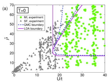
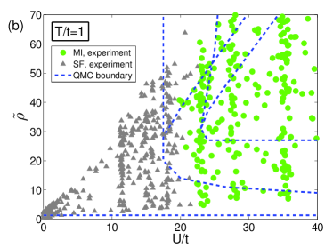
Figure 6: (color online). Comparison of theoretical state diagram boundaries with NIST experimental results of Ref. spielman10, . Circles and triangles represent respectively MI and SF data points from the NIST experiment; same set of data is plotted in (a) and (b). Comparison is made with theoretical state diagram boundaries in (a) $T=0$ and (b) $T/t=1$. The types of coexisting phases for (a) and (b) are given in Fig. 4. There are MI points for low values of $\tilde{\rho}$ in (a) that are below the state diagram boundary $\tilde{\rho}\approx 18$. For finite-T, the state diagram boundary goes down as in (b) containing many of these MI/N data points. We identify this feature as a finite temperature effect fully explainable with a finite-T state diagram.

In a recent experiment at NIST spielman10 , the state diagram for a 2D harmonically trapped lattice system was obtained by measuring the condensate fraction to identify the superfluid and Mott insulator regions as a function of atom density and lattice depth. By comparing to the $T=0$ QMC state diagram, they have shown the breakdown of LDA, indicated by the appearance of MI shoulders for higher values of $(U/t)_{\rm c}$ than a homogeneous system; a phenomenon illustrated in our theory study here in Fig. 4(a).

In Figs. 6(a) and (b) we show respectively the $T=0$ and $T/t=1$ state diagrams of Figs. 4(a) and (b) overlaid with the experimental data points of the NIST experiment; the circles represent MI and the triangles SF. We do not show the experimental phase boundary and its uncertainty reported in Ref. spielman10, . Although the experimental comparison was done with a $T=0$ state diagram, the temperature was reported to be $T/t=0.9(2)$, considered a low enough temperature for such a comparison. However, as we have seen in Figs. 4(a) and (b), because of the appearance of normal phase regions in the cloud, the state diagram at $T/t=1$ begin to differ from $T=0$. Here we choose to overlay the experimental data both in our $T=0$ and $T/t=1$ state diagrams (same data in both panels in Fig. 6). It is visually quite clear that the experiment obtains SF points for low $U/t$ and MI points for high $U/t$. However, the transition occurs at different values of $U/t$ for different $\tilde{\rho}$ in the vertical axis, shown more clearly in the phase boundary plotted in Ref. spielman10, , signifying breakdown of LDA.

We find that for MI points in low $\tilde{\rho}$, the data agrees more with the state diagrams at $T/t=1$ than at $T=0$. For low $\tilde{\rho}$ the measurement of different phases is difficult due to increased thermal fluctuations, and the measurement uncertainty is large. In Fig. 6(a), there appear many MI points below the boundary of $\tilde{\rho}\approx 18$. In Fig. 6(b), we see that the lower boundary for MI/N goes down to $\tilde{\rho}\approx 9$ containing many of these points. We should emphasize that the reported experiment temperature of $T/t=0.9$ is the initial temperature, while the final temperature during the measurement is unknown and could be higher, and in such a case, the boundary would go further down containing all the experimental MI/N data points. With the results of MI points below the lower boundary for $T=0$, we would argue that the experiment was able to detect a finite temperature effect, fully explainable with a finite-T state diagram. We would like to point out that with time of flight imaging of momentum distribution and measuring of condensate fraction, the distinction that is made in the experiment between SF and MI at $T=0$ is the same as the distinction between SF and N/MI at finite temperature.

IV.5 Role of LDA-derived superfluid density in the state diagram

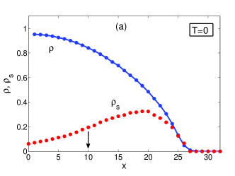
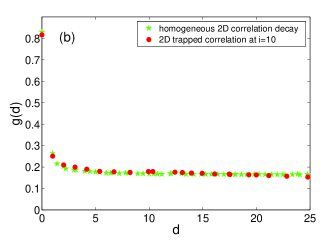
Figure 7: (color online). (a) Density profile and local superfluid density for trapped atoms when the whole region is SF for parameters $t/U=0.025$, $T/t=1/8$, $V_{T}/t=0.012$ and $\mu_{center}/U=0.1$. In (b) circles show the correlation decay between a point $i=10$ and other points along the circumference of radius $i=10$, as a function of the arc distance $d$. The pentagrams show correlation decay for a 2D uniform system for a chemical potential same as that in the trapped system at $i=10$. Since they match very well, we can conclude that the effect of trapping has not changed the long range correlations in this special case when the SF region is wide enough.

The phase boundaries for finite temperature state diagrams in Fig. 4(b) and (c) were obtained determining the density profile and compressibility with QMC simulations of a confined system. In addition to these two quantities, and in the absence of a definition of the local superfluid, LDA-derived $\rho_{s}$ was used to determine the trapped superfluid region as has been assumed in the literature zhou09 ; ho09 . In next section we study bosonic Green’s function which measures the off-diagonal long range order, and by comparing trapped correlations with homogeneous (LDA) correlations, we find that LDA does not correctly capture the trapped superfluid properties. For SF rings of narrow width, correlation decay do not match a 2D decay, and therefore assigning local $\rho_{s}$ values from a 2D homogeneous system has limited validity. So the state diagram boundaries we have obtained here give the upper limit boundaries of confined phases. This is only true for the regions where there are SF rings. High temperature state diagram such as at $T/t=2$ in Fig. 4(c), where no SF rings can form, the phase boundaries are not influenced by this. In Figs. 4(a) and (b), for regions with SF rings, the superfluid designation with LDA-derived $\rho_{s}$ has to be kept in mind. At $T=0$ and $T/t=1$, the SF rings are 1D superfluids or a crossover between 1D and 2D.

To be clear, there can be two LDA issues; one is due to finite size, and another one is in the description of superfluid properties in trapped rings with LDA $\rho_{s}$, an effect we identify in next section. Since QMC simulations in a trap were used for density and compressibility, we do not have the finite-size LDA issue related to the appearance of MI shoulders like in $T=0$ diagram in Fig. 4(a). It is the use of local LDA $\rho_{s}$ to designate the phases, for which we would like to qualify our state diagrams by the fact that in the regions where there are annular SF rings, they can exhibit true long-range order or quasi-long-range order depending on the width of the ring.

V Correlation function at zero and finite temperature

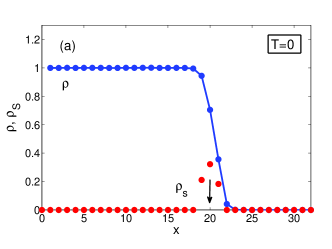
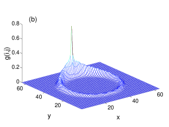
Figure 8: (color online). The effect of reduced dimensionality in a trapped superfluid ring. Panel (a) depicts a narrow SF ring of only 4 sites in width, for parameters $t/U=0.025$, $T/t=1/8$, $V_{T}/t=0.07$ and $\mu_{center}/U=0.7$. 3D plot of $g(i,j)$ for $i=20$ is shown in (b), where we see that $g(i,j)$ is nonzero all across the ring. However, a comparison with the homogeneous correlations in (c) reveals that the trapped decay (circles) is faster in the ring than a true 2D decay (pentagrams), matching only for a very small distance. In (c) we also compare trapped ring correlations with a 1D correlation decay (triangles) at the same parameters and temperature $T/t=1/8$, and find that the 1D algebraic SF decay is faster. This demonstrates that the bose gas in the incommensurate ring is in a crossover regime between 1D and 2D. Assigning 2D LDA $\rho_{s}$ values to the trapped rings therefore has limited validity, pointing out a breakdown of LDA in describing superfluid properties in a trap.

Figure 9: (color online). The behavior of spatial correlations for trapped superfluids at finite temperature. For the parameters $T/t=1$, $\mu/U=0.4$, $t/U=0.05$ and $V_{T}/t=0.4$, (a) shows the density profile and local superfluid density indicating a superfluid ring of finite width. (b) plots $g(i,j)$ between the point $i=20$ and the rest of the lattice, showing clearly that although $i=20$ is SF according to LDA picture, the decay is such that there is no long-range order along the entire ring. (c) quantifies the decay in greater depth – the circles showing the correlation along the ring slowly going to zero at a large distance. $g(i,j)$ for a homogeneous 2D superfluid with the same parameters is given in pentagrams. The triangles, 1D correlation at the same density and temperature $T/t=1$, decays much faster. However, the diamonds depicting 1D correlations at a much lower temperature ($T/t=1/8$) are seen to be similar to that of the 2D trapped annular SF correlations at $T/t=1$. This suggests that for the purpose of long range properties the quasi-1D ring is at a much lower effective temperature than the equilibrium temperature of the 2D atomic cloud. For normal region at $i=15$, the 2D homogeneous correlations match as shown in (d).

To further analyze the trapped system, we study spatial correlations in the trap by looking at the one-particle density matrix between bosons on site $i$ and $j$, $g(i,j)=\langle a^{\dagger}_{i}a_{j}\rangle$. As shown in previous section, the harmonic trap at zero and low enough temperature creates a superfluid ring surrounding the Mott insulating or normal region. The SF ring, having a finite width and a relatively longer length around a circle, has a quasi-1D geometry.

For the parameters $\mu/U=0.1$, $t/U=0.025$, $V_{T}/t=0.012$, and zero temperature ($T/t=1/8$), Fig. 7(a) shows the density profile of trapped atoms where the whole region is SF. The red circles in (a) are local superfluid densities obtained by LDA. In Fig. 7(b), we plot the trapped correlation function decay (circles) between a point at $i=10$ and all points along the ring at the same radius, as a function of their distance $d$. Since the circular ring has the same local chemical potential at all points, we can take a homogeneous system with that specified chemical potential, and make a meaningful comparison with the trapped correlation function as we do in LDA for variables such as density, compressibility, etc. Such a homogeneous correlation decay shown in pentagram symbols match very well the trapped $g(i,j)$ decay. This implies that the effect of trapping (inhomogeneity) has not changed the behavior of long-range correlations; this is true in this specific example where the SF region is wide enough that it retains its 2D superfluid properties, as we will soon show that trapping does have an effect on the SF rings of quasi-1D geometry.

In Fig. 8, we investigate the zero temperature ($T/t=1/8$) correlations for a narrow SF ring. Panel (a) shows the density profile and local superfluid density indicating that the ring is approximately 4 sites in width. Panel (b) shows a 3D plot of $g(i,j)$ for a point in the SF ring, between $i=20$ and for all other sites $j$ in the lattice. It is evident that order persists all across the narrow ring as $g(i,j)$ is nonzero along the circle, whereas it decays rapidly to zero radially from the SF region to the MI plateau. Similar to Fig. 7(b), in Fig. 8(c) we compare the trapped correlation decay for $i=20$ along the ring (circles) to the homogeneous correlations at the same $\mu$ (pentagrams). It shows that the trapped SF decay matches the homogeneous decay for a short distance, after which it continues to deviate from a 2D SF decay. Thus the SF ring does not have 2D superfluid properties, rather it exhibits quasi-long-ranged correlations, influenced by the width of the ring. So the trapped annular SF decay not matching a 2D SF decay, we can find out whether it might match a 1D correlation decay, since the ring has a finite width. In Fig. 8(c) we compare 2D trapped correlations along the ring with 1D homogeneous correlation decay (triangles) at the same density and temperature, $T/t=1/8$. In 1D, the decay is algebraic ($|i-j|^{-p}$, $p$ is the decay exponent, a positive real number) for superfluid and exponential ($e^{-|i-j|/\xi}$, $\xi$ is correlation length) for a Mott or normal phase kollath04 ; rigol04 ; cirac08a . We see in (c) that the 2D ring correlations decay slower than a homogeneous 1D algebraic SF decay but faster than a homogeneous 2D decay. We can therefore conclude that the bose gas in the SF ring is in a crossover regime between a 1D and 2D superfluid. As the width narrows, it would approach a 1D SF decay, and as the width increases, as we have seen in the earlier example, the trapped correlation decay would approach a 2D SF decay.

While all these may seem quite intuitive because of the quasi-1D nature of the ring, the significance of these results is in the fact that assigning 2D LDA-derived local superfluid density to the ring, as have been assumed in many recent papers zhou09 ; fang10 and in previous section, is not totally justified. It indicates a breakdown of LDA for local condensate properties. We know that for trapped atomic systems, LDA describes very well the local density dependent quantities, such as density, variance and compressibility zhou09 ; batrouni08 . A known failure of LDA in trapped systems is due to finite size effects in determining the appearance of a phase boundary rigol09 ; spielman10 . We show here that the effect of reduced dimensionality in traps lead to another failure – in the LDA description of local superfluid density in the trapped annular rings.

Fig. 9 illustrates the behavior of spatial correlations at finite temperature which is one of the key results of this article. For the parameters $T/t=1$, $\mu/U=0.4$, $t/U=0.05$ and $V_{T}/t=0.4$, Fig. 9(a) shows the density profile and local superfluid density exhibiting a superfluid ring of finite width. Fig. 9(b) plots $g(i,j)$ between the point $i=20$ and other points on the lattice, showing clearly that although $i=20$ is SF according to LDA picture, the decay is such that there is no long-range order across the entire ring. Fig. 9(c) quantifies the decay in greater depth – the circles showing the correlation along the ring slowly going to zero at a large distance. For a homogeneous 2D superfluid with the same $t/U$, $T/t$, and at the same $\mu$ as the spatial location $i=20$, the correlation is shown in pentagrams, where the decay is correctly that of a 2D SF. 1D correlation at the same temperature $T/t=1$ and parameters, shown in triangles, decays much faster. However, the diamonds depicting 1D correlations at a much lower temperature $T/t=1/8$ are seen to be qualitatively similar to that of 2D trapped annular ring at $T/t=1$. This implies that as far as the long range properties are concerned, the annular ring is at a lower effective temperature than the 2D cloud. This may be due to reduced fluctuations induced by the collective behavior of a finite width ring. In Fig. 9(d) we show correlations in trapped normal region at $i=15$ where it matches with the 2D homogeneous correlations.

VI Conclusion

In this paper, we determined the combined effects of harmonic trapping and temperature for a square lattice Bose-Hubbard model to obtain the finite temperature state diagram. This extends previous workrigol09 which examined phase coexistence at $T=0$. As temperature increases, thermal fluctuations melt away both the SF and MI phases, introducing the N phase. At finite-T, the N liquid phase is always present in a trap, in the lower density regions furthest from the trap center. Furthermore, each SF and MI region is surrounded by a N ring. This gives rise to many different confined phases. As the temperature increases, the critical coupling $(U/t)_{\rm c}$ for the SF-N transition is lowered and the MI-N crossover coupling is increased. For the phases that contain SF annular rings in the state diagram, the quasi-long range nature of their correlations have to be kept in mind. In addition to the trapped state diagram, we presented the homogenous system phase diagram at finite temperature, for temperature in units of both $T/t$ and $T/U$.

We compare our state diagrams to a recent experiment at NIST spielman10 done on a harmonically trapped 2D lattice. Although the experiment mainly focused on reporting the breakdown of LDA in obtaining the critical coupling, we identify that they have also observed signatures of finite-T in the state diagram.

To further understand the trapped phases, we examine the dependence of spatial correlations $g(i,j)$ in the annular superfluid ring. We show that the correlation decay in SF rings does not match the 2D homogeneous superfluid at the same parameters. For short distances, on the order of the width of the ring, the correlations agree, while for longer distances the deviation gets bigger. At zero temperature, the correlation decay is intermediate between 1D and 2D decay. At finite temperature, the trapped correlation decay rate is much faster than a homogeneous 2D decay. Although it is still slower than a 1D decay at the same temperature, 1D correlations at a much lower temperature matches the trapped decay. This indicates that the ring is at a lower effective temperature, a fact that may have important consequences for long range properties in lower dimensions. These studies point out the fact that assigning LDA $\rho_{s}$ values to the trapped SF rings has limited validity, and thus provide evidence for the breakdown of the local density approximation (LDA) in the description of superfluid properties of trapped bosons.

The quantitative values for the phase boundaries provided here provide numerical benchmarks for continuing efforts to emulate the Bose-Hubbard model on optical lattices, and demonstrate experimental-theoretical consistency for the numerical values of the location of the critical points.

- (1) M. Greiner, O. Mandel, T. Esslinger, T. W. Hänsch and I. Bloch, Nature 415, 39 (2002).
- (2) D. Jaksch, C. Bruder, J. I. Cirac, C. W. Gardiner, and P. Zoller, Phys. Rev. Lett. 81, 3108 (1998).
- (3) M. Lewenstein, A. Sanpera, V. Ahufinger, B. Damski, A. Sen, and U. Sen, Advances in Physics 56, 243 (2007).
- (4) I Bloch, J. Dalibard, and W. Zwerger, Rev. Mod. Phys. 80, 885-964 (2008).
- (5) K. Jimenez-Garcia, R. L. Compton, Y.-J. Lin, W. D. Phillips, J. V. Porto, and I. B. Spielman, Phys. Rev. Lett. 105, 110401 (2010).
- (6) I. B. Spielman, W. D. Phillips, and J. V. Porto, Phys. Rev. Lett. 98, 080404 (2007); Phys. Rev. Lett. 100, 120402 (2008).
- (7) S. Trotzky, L. Pollet, F. Gerbier, U. Schnorrberger, I. Bloch, N. V. Prokof’ev, B. Svistunov, and M. Troyer, Nat. Phys. 6, 998 (2010).
- (8) G. G. Batrouni, R. T. Scalettar, and G. T. Zimanyi, Phys. Rev. Lett. 65, 1765 (1990).
- (9) W. Krauth and N. Trivedi, Europhys. Lett. 14, 627 (1991).
- (10) J. K. Freericks and H. Monien, Phys. Rev. B 53, 2691 (1996); N. Elstner and H. Monien, Phys. Rev. B 59, 12184 (1999).
- (11) B. Capogrosso-Sansone, S. G. Söyler, N. Prokof’ev, and B. Svistunov, Phys. Rev. A 77, 015602 (2008).
- (12) M. Rigol, G. G. Batrouni, V. G. Rousseau and R. T. Scalettar, Phys. Rev. A 79, 053605 (2009).
- (13) N. Gemelke, X. Zhang, C.-L. Hung, and C. Chin, Nature 460, 995 (2009).
- (14) C.-L. Hung, X. Zhang, N. Gemelke, and C. Chin, Phys. Rev. Lett. 104, 160403 (2010).
- (15) W. S. Bakr, J. I. Gillen, A. Peng, S. Foelling, and M. Greiner, Nature 462, 74 (2009).
- (16) J. F. Sherson, C. Weitenberg, M. Endres, M. Cheneau, I. Bloch, and S. Kuhr, Nature 467, 68 (2010).
- (17) G. Pupillo, C. J. Williams, and N. V. Prokof ev, Phys. Rev. A. 73, 013408 (2006).
- (18) L. Pollet, C. Kollath, K. Van Houcke, and M. Troyer, New J. Phys. 10 065001 (2008).
- (19) T. -L. Ho and Q. Zhou, Phys. Rev. Lett 99, 120404 (2007).
- (20) K. W. Mahmud, G. G. Batrouni, and R. T. Scalettar, Phys. Rev. A 81, 033609 (2010).
- (21) F. Gerbier, Phys. Rev. Lett. 99, 120405 (2007).
- (22) B. DeMarco, C. Lannert, S. Vishveshwara, and T.-C. Wei, Phys. Rev. A 71, 063601 (2005).
- (23) S. Wessel, F. Alet, M. Troyer, and G. G. Batrouni, Phys. Rev. A 70, 053615 (2004).
- (24) Q. Zhou, Y. Kato, N. Kawashima, and N. Trivedi, Phys. Rev. Lett. 103, 085701 (2009).
- (25) Y. Kato, Q. Zhou, N. Kawashima, and N. Trivedi, Nature Phys. 4, 617 (2008).
- (26) T. Roscilde, arXiv1003.4005.
- (27) L. Pollet, N. V. Prokof’ev, and B. V. Svistunov, Phys. Rev. Lett. 104, 245705 (2010).
- (28) S. Fang, C.-M. Chung, P. N. Ma, P. Chen, and D.-W. Wang, arXiv:1009.5155.
- (29) Kaden R. A. Hazzard and Erich J. Mueller, arXiv:1006.0969.
- (30) P. N. Ma, L. Pollet, and M. Troyer, Phys. Rev. A 82, 033627 (2010).
- (31) G. G. Batrouni, V. Rousseau, R. T. Scalettar, M. Rigol, A. Muramatsu, P. J. H. Denteneer, and M. Troyer, Phys. Rev. Lett. 89, 117203 (2002).
- (32) M. P. A. Fisher, P. B. Weichman, G. Grinstein, and D. S. Fisher, Phys. Rev. B 40, 546 (1989).
- (33) To make a dimensionality independent connection, the hopping term is sometimes written as , where is the number of nearest neighbor sites, for 1D, for 2D and for 3D hypercubic lattices kato08 . Since we are strictly focusing on 2D, we analyze our results in the convention the experimentalists usecchin09 ; spielman10 as given in the Hamiltonian in Eq. 1.
- (34) Y. Kato, T. Suzuki and N. Kawashima, Phys. Rev. E, 75, 66703 (2007); Y. Kato and N. Kawashima, Phys. Rev. E, 79, 21104 (2009).
- (35) N. Kawashima and K. Harada, J. Phys. Soc. Jpn., 73, 1379–1414 (2004).
- (36) K. Sheshadri, H. R. Krishnamurthy, R. Pandit, and T. V. Ramakrishnan, Europhys. Lett. 22, 257 (1993).
- (37) X. Lu and Y. Yu, Phys. Rev. A 74, 063615 (2006).
- (38) P. Buonsante and A. Vezzani, Phys. Rev. A 70, 033608 (2004).
- (39) T. P. Polak and T. K. Kopec, J. Phys. B 42 095302 (2009).
- (40) Matthias Ohliger and Axel Pelster, arXiv:0810.4399.
- (41) G. G. Batrouni, H. R. Krishnamurthy, K. W. Mahmud, V. G. Rousseau, and R. T. Scalettar, Phys. Rev. A 78, 023627 (2008).
- (42) Tin-Lun Ho and Qi Zhou, Nature Physics 6, 131 (2009).
- (43) C. Kollath, U. Schollwöck, J. von Delft, and W. Zwerger, Phys. Rev. A 69, 031601(R) (2004).
- (44) M. Rigol and A. Muramatsu, Phys. Rev. A 70, 031603 (2004).
- (45) X.-L. Deng, D. Porras, and J. I. Cirac, Phys. Rev. A 77, 033403 (2008).