Study of the spectral properties of spin ladders in different representations via a renormalization procedure

Abstract

We implement an algorithm which is aimed to reduce the dimensions of the Hilbert space of quantum many-body systems by means of a renormalization procedure. We test the role and importance of different representations on the reduction process by working out and analyzing the spectral properties of strongly interacting frustrated quantum spin systems.

PACS numbers: 02.70.-c; 03.65.-w; 05.10.Cc; 71.27.+a

Keywords: Effective theories, renormalization, strongly interacting systems, quantum spin systems.

1 Introduction.

Most microscopic many-body quantum systems are subject to strong interactions which act between their constituents. In general, there exist no analytical methods to treat exactly strongly interacting systems apart from the assumption of trial wave functions able to diagonalize the Hamiltonian of integrable models, like the Bethe Ansatz $(BA)$ for specific one dimensional systems $(1D)$ [1], the $BCS$ hypothesis which explains the supraconductivity and others like the Néel state, the Resonant Valence Bond ($RVB$) spin liquid states proposed by Anderson [2], the Valence Bond Crystal states ($VBC$)…. They are aimed to describe $2D$ systems but there remains the problem of their degree of realism, i.e. their ability to include the essentials of the interaction in strongly interacting systems  [3]. The complexity of the structure of such systems leads to the diagonalization of the Hamiltonian numerically which must in general be performed in very large Hilbert space although the information of interest is restricted to the knowledge of a few low energy states generally characterized by collective properties. Consequently it is necessary to manipulate very large matrices in order to extract a reduced quantity of informations.

Non-perturbative techniques are needed. During the last decades a considerable amount of procedures relying on the renormalization group concept introduced by Wilson  [4] have been proposed and tested. Some of them are specifically devised for quantum spin systems, like the Real Space Renormalization Group (RSRG) [5, 6] and the Density Matrix Renormalization Group (DMRG)  [7, 8].

We propose here a non-perturbative approach which tackles this question  [9]. The procedure consists of an algorithm which implements a step by step reduction of the size of Hilbert space by means of a projection technique. It relies on the renormalization concept following in spirit former work based on this concept [10, 11, 12]. Since the reduction procedure does not act in ordinary or momentum space but in Hilbert space, it is universal in the sense that it works for any kind of many-body quantum system.

The properties of physical systems can be investigated in different representations. In the present work which deals with frustrated spin ladders the common $SU(2)$-representation is confronted with the $SO(4)$-representation  [13, 14, 15] in order to work out the energies of the low-lying levels of the spectrum of these systems. The efficiency of one or the other representation in terms of the number of relevant basis states characterizing the ground state wave function is tested in connection with the reduction process.

The outline of the paper is the following. In section $2$ we present the formal developments leading to the secular equation in the reduced Hilbert space. Section $3$ is devoted to the application of the algorithm to frustrated quantum spin ladders with two legs and one spin per site. We analyze the outcome of the applied algorithm on systems characterized by different coupling strengths by means of numerical examples, in bases of states developed in the $SU(2)$ and $SO(4)$-representations and compare the results obtained in both cases. Conclusions and further possible investigations and developments are presented in section $4$.

2 The reduction algorithm.

2.1 Reduction procedure and renormalization of the coupling strengths.

We consider a system described by a Hamiltonian depending on a unique coupling strength $g$ which can be written as a sum of two terms

$$H=H_{0}+gH_{1}\$$ (1)

The Hilbert space ${\cal H}^{(N)}$ of dimension $N$ is spanned by an orthonormalized arbitrary set of basis states $\left\{|\Phi_{i}\rangle,\,i=1,\cdots,N\right\}$. In this basis an eigenvector $|\Psi_{l}^{(N)}\rangle$ takes the form

$$|\Psi_{l}^{(N)}\rangle=\sum_{i=1}^{N}a_{li}^{(N)}(g^{(N)})|\Phi_{i}\rangle\$$ (2)

where the amplitudes $\{a_{li}^{(N)}(g^{(N)})\}$ depend on the value $g^{(N)}$ of $g$ in ${\cal H}^{(N)}$.

Using the Feshbach formalism [16] the Hilbert space may be decomposed into subspaces by means of the projection operators $P$ and $Q$,

$${\cal H}^{(N)}=P{\cal H}^{(N)}+Q{\cal H}^{(N)}$$ (3)

In practice the subspace $P{\cal H}^{(N)}$ is chosen to be of dimension $\mathrm{dim}\,P{\cal H}^{(N)}=N-1$ by elimination of one basis state. The projected eigenvector $P|\Psi_{l}^{(N)}\rangle$ obeys the Schroëdinger equation

$$H_{eff}(\lambda_{l}^{(N)})P|\Psi_{l}^{(N)}\rangle=\lambda_{l}^{(N)}P|\Psi_{l}^{(N)}\rangle\ .$$ (4)

where $H_{eff}(\lambda_{l}^{(N)})$ is the effective Hamiltonian which operates in the subspace $P{\cal H}^{(N)}$. It depends on the eigenvalue $\lambda_{l}^{(N)}$ which is the eigenenergy corresponding to $|\Psi_{l}^{(N)}\rangle$ in the initial space ${\cal H}^{(N)}$. The coupling strengths $g^{(N)}$ which characterizes the Hamiltonian $H^{(N)}$ in ${\cal H}^{(N)}$ is now aimed to be changed into $g^{(N-1)}$ in such a way that the eigenvalue in the new space ${\cal H}^{(N-1)}$ is the same as the one in the complete space

$$\lambda_{l}^{(N-1)}=\lambda_{l}^{(N)}\$$ (5)

The determination of $g^{(N-1)}$ by means of the constraint expressed by Eq. (5) is the central point of the procedure. It is the result of a renormalization procedure induced by the reduction of the vector space of dimension $N$ to $N-1$ which preserves the physical eigenvalue $\lambda_{l}^{(N)}$.

In the sequel $P|\Psi_{1}^{(N)}\rangle$ is chosen to be projection of the ground state eigenvector $|\Psi_{1}^{(N)}\rangle$ $(l=1)$ and $\lambda_{1}^{(N)}=\lambda_{1}^{(N-1)}=\lambda_{1}$ the corresponding eigenenergy. In ref. [9] it is shown how $g^{(N-1)}$ can be obtained as a solution of an algebraic equation of the second degree. One gets explicitly a discrete quadratic equation

$${a^{(N-1)}{g^{(N-1)}}^{2}+b^{(N-1)}g^{(N-1)}+c^{(N-1)}}=0\$$ (6)

where

$$a^{(N-1)}=G_{1N}-H_{NN}F_{1N}\$$ (7)

$$b^{(N-1)}=a_{11}^{(N)}H_{NN}(\lambda_{1}^{(N)}-\alpha_{1})+F_{1N}(\lambda_{1}^{(N)}-\alpha_{N})\$$ (8)

$$c^{(N-1)}=-a_{11}^{(N)}(\lambda_{1}^{(N)}-\alpha_{1})(\lambda_{1}^{(N)}-\alpha_{N})\$$ (9)

with

$$F_{1N}=\sum_{i=1}^{N-1}a_{1i}^{(N)}\langle\Phi_{1}|H_{1}|\Phi_{i}\rangle$$

$$G_{1N}=H_{1N}\sum_{i=1}^{N-1}a_{1i}^{(N)}\langle\Phi_{N}|H_{1}|\Phi_{i}\rangle$$

$$H_{ij}=\langle\Phi_{i}|H_{1}|\Phi_{j}\rangle$$

and

$$\alpha_{i}=\langle\Phi_{i}|H_{0}|\Phi_{i}\rangle,\,i=1,\cdots,N$$

The reduction procedure is then iterated in a step by step decrease of the dimensions of the vector space, $N\mapsto N-1\mapsto N-2\mapsto...$ leading at each step $k$ to a coupling strength $g^{(N-k)}$ which can be given as the solution of a flow equation in a continuum limit description of the Hilbert space. The procedure can be generalized to Hamiltonians depending on several coupling constants which experience a renormalization during the reduction procedure under further constraints [18].

2.2 Outline of the reduction algorithm.

We sketch here the different steps of the procedure.

$1-$ Consider a quantum system described by an Hamiltonian $H^{(N)}$ which acts in an $N$-dimensional Hilbert space.

$2-$ Compute the matrix elements of the Hamiltonian matrix $H^{(N)}$ in a definite basis of states $\{|\Phi_{i}\rangle,i=1,\ldots,N\}$. The diagonal matrix elements $\{\epsilon_{i}=\langle\Phi_{i}|H^{(N)}|\Phi_{i}\rangle\}$ are arranged either in increasing order with respect to the $\{\epsilon_{i}\}$ or in decreasing order of the absolute values of the ground state wave function amplitudes $|a_{1i}^{(N)}(g^{(N)})|$ [17].

$3-$ Use the Lanczos technique to determine $\lambda_{1}^{(N)}$ and $|\Psi_{1}^{(N)}(g^{(N)})\rangle$ [19, 20].

$4-$ Fix $g^{(N-1)}$ as described in section 2.1. Take the solution of the algebraic second order equation closest to $g^{(N)}$ (see Eq.(6)).

$5-$ Construct $H^{(N-1)}=H_{0}+g^{(N-1)}H_{1}$ by elimination of the matrix elements of $H^{(N)}$ involving the state $|\Phi_{N}\rangle$.

$6-$ Repeat procedures $3$, $4$ and $5$ by fixing at each step $k$ $\{k=1,\ldots,N-N_{min}\}$, $\lambda_{1}^{(N-k)}=\lambda_{1}^{(N)}=\lambda_{1}$. The iterations are stopped at $N_{min}$ corresponding to the limit of space dimensions for which the spectrum gets unstable.

2.3 Some remarks.

• The procedure is aimed to generate the energies of the low-energy excited states of strongly interacting systems and possibly the calculation of further physical quantities.

• The implementation of the reduction procedure asks for the knowledge of $\lambda_{1}$ and the corresponding eigenvector $|\Psi_{1}^{(N-k)}\rangle$ at each step $k$ of the reduction process. The eigenvalue $\lambda_{1}$ is chosen as the physical ground state energy of the system. Eigenvalue and eigenvector can be obtained by means of the Lanczos algorithm  [8, 19, 20] which is particularly well adapted to very large vector space dimensions. The algorithm fixes $\lambda_{1}^{(N-k)}=\lambda_{1}^{(N)}$ and determines $|\Psi_{1}^{(N-k)}\rangle$ at each step.
  

• The process does not guarantee a rigorous stability of the eigenvalue $\lambda_{1}$. $|\Psi_{1}^{(N-k-1)}\rangle$ which is the eigenvector in the space ${\cal H}^{(N-k-1)}$ and the projected state $P|\Psi_{1}^{(N-k)}\rangle$ of $|\Psi_{1}^{(N-k)}\rangle$ into ${\cal H}^{(N-k-1)}$ may differ from each other. As a consequence it may not be possible to keep $\lambda_{1}^{(N-k-1)}$ rigorously equal to $\lambda_{1}^{(N-k)}=\lambda_{1}$. In practice the degree of accuracy depends on the relative size of the eliminated amplitudes $\{a_{1(N-k)}^{(N-k)}(g^{(N-k)})\}$. This point will be tested by means of numerical estimations and further discussed below.
  

• The Hamiltonians of the considered ladder systems are characterized by a fixed total magnetic magnetization $M_{tot}$. We work in subspaces which correspond to fixed $M_{tot}$. The total spin $S_{tot}$ is also a good quantum number which defines smaller subspaces for fixed $M_{tot}$ [21]. We do not introduce them here because projection procedures on $S_{tot}$ are time consuming. Furthermore we want to test the algorithm in large enough spaces although not necessarily the largest possible ones in this preliminary tests considered here.

3 Application to frustrated two-leg quantum spin ladders.

3.1 The model

3.1.1 SU(2)-representation.

Consider spin-$1/2$ ladders [22, 23] described by Hamiltonians of the following type and shown in $Fig.1$

$$H^{(s,s)} = J_{t}\sum_{i=1}^{L}s_{i_{1}}s_{i_{2}}+J_{l}\sum_{<ij>}s_{i_{1}}s_{j_{1}}+J_{l}\sum_{<ij>}s_{i_{2}}s_{j_{2}}+J_{1c}\sum_{(ij)}s_{i_{1}}s_{j_{2}}$$

$$+J_{2c}\sum_{(ij)}s_{i_{2}}s_{j_{1}}$$

Figure 1: Top: the original spin ladder. The coupling strengths are indicated as given in the text. Bottom: The ladder in the SO(4)-representation. See the text.

The indices $1$ or $2$ label the spin $1/2$ vector operators $s_{i_{k}}$ acting on the sites $i$ on both ends of a rung, in the second and third term $i$ and $j$ label nearest neighbours, here $j=i+1$ along the legs of the ladder. The fourth and fifth term correspond to diagonal interactions between sites located on different legs, $j=i+1$. $L$ is the number of sites on a leg (Fig. 1) where $J_{1c}=J_{2c}=J_{c}$. The coupling strengths $J_{t},J_{l},J_{c}$ are positive.

As stated above the renormalization is restricted to a unique coupling strength, see Eq. (1). It is implemented here by putting $H_{0}=0$ and $H^{(N)}=g^{(N)}H_{1}$ where $g^{(N)}=J_{t}$ and

$$H_{1}=\sum_{i=1}^{L}s_{i_{1}}s_{i_{2}}+\gamma_{tl}\sum_{<ij>}(s_{i_{1}}s_{j_{1}}+s_{i_{2}}s_{j_{2}})+\gamma_{c}\sum_{<ij>}(s_{i_{1}}s_{j_{2}}+s_{i_{2}}s_{j_{1}})\ .$$ (11)

where $\gamma_{tl}=J_{l}/J_{t}$, $\gamma_{c}=J_{c}/J_{t}$. These quantities are kept constant and $g^{(N)}=J_{t}$ will be subject to renormalization during the reduction process.

One should point out that the renormalization does not change if one chooses another coupling parameter as a renormalizable parameter, here $J_{l}$ or $J_{c}$, because they are related to each other at the beginning of the reduction procedure by the ratios $\gamma_{tl}=J_{l}/J_{t}$ and $\gamma_{c}=J_{c}/J_{t}$.

The basis of states $\{|\Phi_{p}\rangle\ ,p=1,\ldots,N\}$ is chosen as

$$|\Phi_{p}\rangle=|1/2~{}~{}m_{1},...,1/2~{}~{}m_{i},...,1/2~{}~{}m_{2L},\sum_{i=1}^{2L}m_{i}=M_{tot}=0\rangle$$

with $\{m_{i}=+1/2,-1/2\}$.

3.1.2 SO(4)-representation.

Different choices of bases may induce a more or less efficient reduction procedure depending on the strength of the coupling constants $J_{t},J_{l},J_{c}$. This point is investigated here by choosing also a basis of states which is written in an $SO(4)$-representation.

We replace $(s_{i1},s_{i2})$ corresponding to dimers by $({S_{i}},{R_{i}})$. By means of a spin rotation  [14, 15]

$$s_{i_{1}}=\frac{1}{2}(S_{i}+R_{i})\ .$$ (12)

$$s_{i_{2}}=\frac{1}{2}(S_{i}-R_{i})\ .$$ (13)

The Hamiltonian, Eq. (3.1.1), can be expressed in the form

$$H^{(S,R)}=\frac{J_{t}}{4}\sum_{i=1}^{L}(S_{i}^{2}-R_{i}^{2})+J_{1}\sum_{<ij>}S_{i}S_{j}+J_{2}\sum_{<ij>}R_{i}R_{j}\$$ (14)

The structure of the corresponding system is shown in the lower part of Fig. 1. Here $J_{1}=(J_{l}+J_{c})/2$, $J_{2}=(J_{l}-J_{c})/2$ and as before $J_{1c}=J_{2c}=J_{c}$. The components $S_{i}^{(+)},S_{i}^{(-)},S_{i}^{(z)}$ and $R_{{i}}^{(+)},R_{{i}}^{(-)},R_{{i}}^{(z)}$ of the vector operators $S_{i}$ and $R_{i}$ are the $SO(4)$ group generators and $<ij>$ denotes nearest neighbour indices.

In this representation the states $\{|S_{i}M_{i}\rangle\}$ are defined as

$$|S_{i}M_{i}\rangle=\sum_{m_{1},m_{2}}\langle 1/2~{}~{}m_{1}~{}~{}1/2~{}~{}m_{2}|S_{i}M_{i}\rangle|1/2~{}~{}m_{1}\rangle_{i}|1/2~{}~{}m_{2}\rangle_{i}$$

along a rung are coupled to $S_{i}=0$ or $S_{i}=1$. Spectra are constructed in this representation as well as in the $SU(2)$-representation and the states $\{|\Phi_{p}\rangle\}$ take the form

$$|\Phi_{p}\rangle=|S_{1}M_{1},...,S_{i}M_{i},...,S_{L}M_{L},\sum_{i=1}^{L}M_{i}=M_{tot}=0\rangle$$

3.2 Test observables

In order to quantify the accuracy of the procedure we introduce different test quantities in order to estimate deviations between ground state and low excited state energies in Hilbert spaces of different dimensions. The stability of low-lying states can be estimated by means of

$$p(i)=|\frac{(e_{i}^{(N)}-e_{i}^{(n)})}{e_{i}^{(N)}}|\times 100 with i=1,\ldots,4$$ (15)

where $e_{i}^{(n)}=\lambda_{i}^{(n)}/2L$ with $n=(N-k)$ corresponds to the energy per site at the $i$th physical state starting from the ground state at the $k$th iteration in Hilbert space. This quantity provides a percentage of loss of accuracy of the eigenenergies in the different reduced spaces.

A global characterization of the ground state wavefunction in different representations can also be given by the entropy per site in a space of dimension $n$

$$s=-\frac{1}{2L}\sum_{i=1}^{n}{P_{i}}ln{P_{i}} with P_{i}=|\langle\Phi_{i}^{(n)}|\Psi_{1}^{(n)}\rangle|^{2}=|a_{1i}^{(n)}|^{2}$$ (16)

which works as a global measure of the distribution of the amplitudes $\{a_{1i}^{(n)}\}$ in the physical ground state.

In the remaining part we work out the spectra of different systems and compare results obtained in the two representations introduced above.

3.3 Spectra in the SU(2)-representation.

Results obtained with an $SU(2)$-representation basis of states are shown in $Figs.(2-3)$.

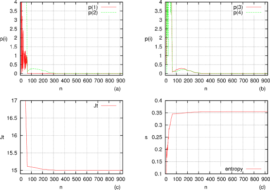
3.3.1 First case: $L$= 6, $J_{t}$=15, $J_{l}$=5, $J_{c}$=3

We choose the basis states in the framework of the $M$-scheme corresponding to subspaces with fixed values of the total projection of the spin of the $\{|\Phi_{i}\rangle\}$, $M_{tot}=0$.

In the present case $J_{t}>J_{l},J_{c}$. The dimension of the subspace is reduced step by step as explained above starting from $N=924$. As stated in section $2.2$ the basis states $\{|\Phi_{i}\rangle\}$ are ordered with increasing energy of their diagonal matrix elements $\{\epsilon_{i}\}$ and eliminated starting from the state with largest energy $\epsilon_{N}$.

Deviations of the energies of the ground and first excited states from their initial values at $N=924$ can be seen in Figs.(2a-b) where the $p(i)$’s defined above represent these deviations in terms of percentages. As seen in Fig.(2a) the ground state of the system stays stable down to $n\sim 50$ where $n$ is the dimension of the reduced space. The coupling constant $J_{t}$ does not move either down to $n\sim 300$, see Fig.(2c). Figs.(2a-b) show the evolution of the first excited states which follows the same trend as the ground state.

For $n\leq 50$ the spectrum gets unstable, the renormalization of the coupling constant can no longer correct for the energy of the lowest state. Indeed the coupling constant $J_{t}$ increases drastically as seen in Fig.(2c). The reason for this behaviour can be found in the fact that at this stage the algorithm eliminates states which have an essential component in the state of lowest energy. The same message can be read on Fig.(2d), the drop in the entropy per site $s$ is due to the elimination of sizable amplitudes $\{a_{1i}\}$.

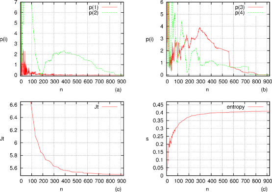
3.3.2 Second case: $L$= 6, $J_{t}$=5.5, $J_{l}$=5, $J_{c}$=3

Contrary to the former case the coupling constant $J_{t}$ along rungs is now of the order of strength as $J_{l},J_{c}$. Results are shown in Fig.(3). The lowest energy state is now stable down to $n\sim 100$. This is also reflected in the behaviour of the excited states which move appreciably for $n\leq 200$. Fig.(3c) shows that the coupling constant $J_{t}$ starts to increase sharply between $n=300$ and $n=200$. It is able to stabilize the excited states down to about $n=200$ and the ground state down to $n=70$. The instability for $n\leq 70$ reflects in the evolution of the $p(i)$’s, Figs.(3a-b) which get of the order of a few percent. The entropy Fig.(3d) follows the same trend.

Comparing the two cases above and particularly the entropies Fig.(3d) and Fig.(2d) one sees that the stronger $J_{t}$ the more the amplitude strength of the ground state wavefunction is concentrated in a smaller number of basis state components. The elimination of sizable components of the wavefunction leads to deviations which can be controlled down to a certain limit by means of the renormalization of $J_{t}$. One sees that large values of $J_{t}$ favour a low number of significative components in the low energy part of the spectrum in a $SU(2)$- representation.

3.3.3 Remark

In Figs.(2a-b) it is seen that the ground and first excited states show ”bunches” of energy fluctuations. In the ground state the peaks are intermittent, they appear and disappear during the space dimension reduction process. They are small in the case where $J_{t}=15$ but can grow with decreasing $J_{t}$ as it can be observed in Figs.(3a-b) for $J_{t}=5.5$. The subsequent stabilization of the ground state energy following such a bunch shows the effectiveness of the coupling constant renormalization which acts in a progressively reduced and hence incomplete basis of states.

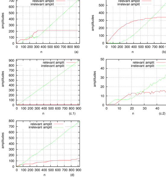
These bunches of fluctuations are correlated with the change of the number of relevant amplitudes (i.e. amplitudes larger than some value $\epsilon$ as explained in the caption of Fig.(6)) during the reduction process.

Consider first the case where $J_{t}>J_{l},J_{c}$. One notices in the caption of Fig.(6a) that down to $n\sim 300$ the number of relevant amplitudes defined in Fig.(6) stays stable like the ratios $\{p(i)\}$ in Figs.(2a-b). For $158<n<300$ these ratios change quickly. A bunch of fluctuations appears in this domain of values of $n$ as seen in Figs.(2a-b) and correspondingly the number of relevant amplitudes decreases steeply. For $60<n\leq 158$ the ratios $\{p(i)\}$ stay again stable as well as the number of relevant amplitudes. The $\{p(i)\}$ in Figs.(2a-b) almost decrease back to their initial values. The analysis shows that these bunches of fluctuations signal the local elimination of relevant contributions of basis states to the physical states in the spectrum. The stabilization of the spectra which follows during the elimination process shows that renormalization is able to cure these effects.

In the case where $J_{t}\sim J_{l},J_{c}$ shown in Fig.(6b) the relevant and irrelevant amplitudes move continuously during the reduction process and the corresponding $\{p(i)\}$ do no longer decrease to the values they showed before the appearance of a bunch of energy fluctuations as seen in Figs.(3a-b). It signals the fact that the coupling renormalization is no longer able to compensate for the reduction of the Hilbert space dimensions.

One should mention that the evolution of the spectrum depends on the initial size of Hilbert space. The larger the initial space the larger the ratio between the initial number of states and the number of states corresponding to the limit of stability of the spectrum, see ref. [18] for explicit numerical examples.

3.4 Spectra in the SO(4)-representation

The reduction algorithm is now applied to the system described by the Hamiltonian $H^{(S,R)}$ given by Eq. (14) with a basis of states written in the $SO(4)$-representation. Like above we consider two cases corresponding to large and close values of $J_{t}$ relative to the strengths of the other coupling parameters.

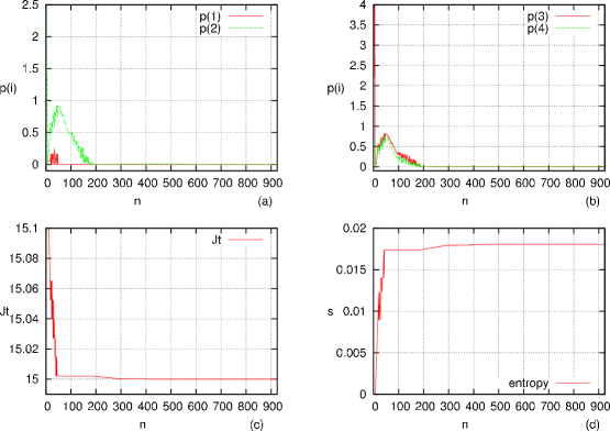
3.4.1 Reduction test for $L=6$, $J_{t}$ = 15, 5.5 and $J_{l}$=5, $J_{c}$=3

Figs.(4-5) show the behaviour of the spectrum for a system of size $L=6$. A large value of $J_{t}$, ($J_{t}=15$), favours the dimer structure along rungs in the lowest energy state and stabilizes the spectrum down to small Hilbert space dimensions. This effect is clearly seen in Fig.(4a), the ground state is very stable. The excited states are more affected, see Fig.(4b), although they do not move significantly. The renormalization of the coupling strength $J_{t}$ starts to work for $n\simeq 50$, Fig.(4c).

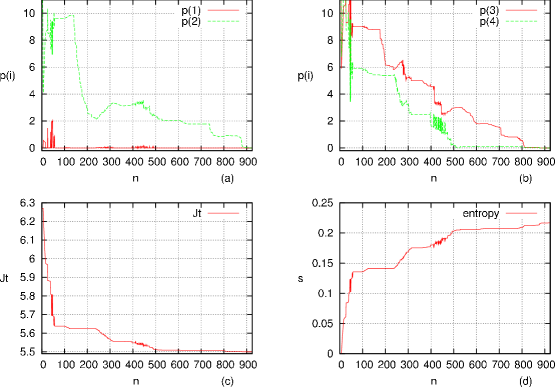
The situation changes progressively with decreasing values of $J_{t}$. Figs.(5) show the case where $J_{t}=5.5$. The ground state energy experiences sizable bunches of fluctuations like in the $SU(2)$-representation, but much stronger than in this last case. The same is true for the excited states which is reflected through all the quantities shown in Figs.(5a-b), in particular $J_{t}$, Fig.(5c). The entropy Figs.(4d,5d) follows the same trend like in the $SU(2)$-representation by changing the values of $J_{t}$ from $15$ to $5.5$. The analysis of the bunches of energy fluctuations through the number of relevant-irrelevant amplitudes is shown for $J_{t}=15$, $J_{l}=5$, $J_{c}=3$ in Fig. (6c.1-c.2) and for $J_{t}=5.5$, $J_{l}=5$, $J_{c}=3$ in Fig. (6d).

The results show that the renormalization procedure is quite sensitive to the representation chosen in Hilbert space. It is expected that essential components of the ground state wavefunction get eliminated early during the process when the rung coupling gets of the order of magnitude or smaller than the other coupling strengths.

By comparing the two representations in Fig(6), one notices that the stability of the low-energy properties of the system in the reduced Hilbert space is well characterized by the number of relevant-irrelevant amplitudes as defined in the caption of Fig.(6) and the distribution of the amplitudes in Hilbert space, see ref. [17].

3.5 Summary

The present results lead to two correlated remarks. The efficiency of the algorithm is different in different sectors of the coupling parameter space. In the case of the frustrated ladders considered here the algorithm is the more efficient the stronger the coupling between rung sites $J_{t}$. Second, this behaviour is strongly related to the representation in which the basis of states is defined. The $SU(2)$-representation leads to a structure of the wave functions (i.e. the size of the amplitudes of the basis states) which is very different from the one obtained in the $SO(4)$-representation. For large values of $J_{t}$ the spectrum is more stable in the $SO(4)$-representation. For small values of $J_{t}$ the stability is better realized in the $SU(2)$- representation. Finally, in the regime where $J_{t}>J_{l},J_{c}$, one observes that the reduction procedure is the more efficient the closer $J_{l}$ to $J_{c}$. This effect can be understood and related to previous analytical work in the $SO(4)$-representation [25].

4 Conclusions and outlook.

In the present work we tested and analysed the outcome of an algorithm which aims to reduce the dimensions of the Hilbert space of states describing strongly interacting systems. The reduction is compensated by the renormalization of the coupling strengths which enter the Hamiltonians of the systems. By construction the algorithm works in any space dimension and may be applied to the study of any microscopic $N$-body quantum system. The robustness of the algorithm has been tested on frustrated quantum spin ladders.

The analysis of the numerical results obtained in applications to quantum spin ladders leads to the following conclusions.

• The present numerical applications are essentially realistic tests of the renormalization algorithm restricted to rather small Hilbert spaces which do not necessarily necessitate the use of a Lanczos procedure. We introduced this procedure in order to be able to extend our present work to much larger systems for which ordinary full diagonalization cannot be performed. We tested it sucessfully by comparing the outcome with that of complete diagonalization. Preliminary extended calculations have also been performed on higher dimensional ladders. We expect to present and discuss the physics of their application to frustrated systems in further work.
  

• The stability of the low-lying states of the spectrum in the course of the reduction procedure depends on the relative values of the coupling strengths. The ladder favours a dimer structure along the rungs, i.e. stability is the better the larger the transverse coupling strength $J_{t}$. This is the reason why the $SO(4)$-representation is favoured when compared to the $SU(2)$- representation in this case. It leads to a more efficient basis of states as commented below (see next paragraph).
  

• The efficiency of the reduction procedure depends on the representation frame in which the basis of states is defined. It appears clearly that the evolution of the spectrum described in an $SU(2)$- representation is significantly different from the evolution in an $SO(4)$-representation. This is understandable since different representations partition Hilbert space in different ways and favour one or the other representation depending on the relative strengths of the coupling constants. It is always appropriate to work in a basis of states whose symmetry properties are closest to the symmetry properties of the physical system so that the contributions of the non-diagonal couplings are the smallest. The choice of an optimal basis may not always be evident. In the case of the ladder we consider here the $SO(4)$-representation.

• Local spectral instabilities appearing in the course of the reduction procedure are correlated with the elimination of basis states with sizable amplitudes in the ground state wavefunction. One or another representation can be more efficient on the reduction process for a given set of coupling parameters because it leads to physical states in which the weight on the basis states is concentrated in a different number of components. This point is strongly related to the correlation between quantum entanglement and symmetry properties which have been under intensive scrutiny, see f.i.  [26] and refs. therein.

Further points are worthwhile to be investigated:

• Extension to larger ladders and systems of higher space dimensions with the help of more sophisticated numerical algorithms  [27, 28].

• Extension of the renormalization procedure to systems at finite temperature  [24] and more than one coupling constant renormalization [18].

Figure 2: $SU(2)-representation$. $n$ is Hilbert space dimension. $L=6$ sites along a leg. $J_{t}=15$, $J_{l}=5$, $J_{c}=3$

Figure 3: $SU(2)-representation$. $n$ is Hilbert space dimension. $L=6$ sites along a leg. $J_{t}=5.5$, $J_{l}=5$, $J_{c}=3$

Figure 4: $SO(4)-representation$. $n$ is Hilbert space dimension. $L=6$ sites along the chain. $J_{t}=15$, $J_{l}=5$, $J_{c}=3$

Figure 5: $SO(4)-representation$. $n$ is Hilbert space dimension. $L=6$ sites along the chain. $J_{t}=5.5$, $J_{l}=5$, $J_{c}=3$

Figure 6: $n$ is the dimension of the Hilbert space. $Amplitudes$ show the number of relevant -irrelevant amplitudes in the ground state eigenfunction (relevant-irrelevant amplit in the figure). Relevant amplitudes are those for which $\{|a_{1i}|>\epsilon$, (here $\epsilon=10^{-2}$), $i=1,\ldots,n\}$. The number of sites along a leg is $L=6$. $SU(2)-representation$: (a) corresponds to $J_{t}=15$, $J_{l}=5$, $J_{c}=3$. (b) corresponds to $J_{t}=5.5$, $J_{l}=5$, $J_{c}=3$. $SO(4)-representation$: (c.1) and (c.2) correspond to $J_{t}=15$, $J_{l}=5$, $J_{c}=3$. (d) corresponds to $J_{t}=5.5$, $J_{l}=5$, $J_{c}=3$.

References

- [1] Indrani Bose, Classical and Quantum Nonlinear Integrable Systems Theory and Application, Chapter 7, Edited by A. Kundu, Taylor and Francis 2003 , Print ISBN: 978-0-7503-0959-2, arXiv:cond-mat/0208039v1
- [2] P. W. Anderson, Science 235 (1987) 1196
- [3] C. Lhuillier and G. Misguish, Frustrated Quantum Magnets, Lecture Notes in Physics, 2002, volume 595/2002, pp.161-190.
- [4] K. G. Wilson, Phys. Rev. Lett. 28 (1972) 548; Rev. Mod. Phys. 47 (1975) 773
- [5] Jean-Paul Malrieu and Nathalie Guithéry, Phys.Rev. B63 (1998)085110
- [6] S. R. White and R. M. Noack, Phys. Rev. Lett. 68 (1992) 3487
- [7] S. R. White, Phys. Rev. Lett. 69 (1992) 2863
- [8] M. Henkel, Conformal invariance and critical phenomena, Springer Verlag, 1999
- [9] T. Khalil and J. Richert, J. Phys. A: Math. Gen. 37 (2004) 4851-4860
- [10] S. D. Glazek and Kenneth G. Wilson, Phys. Rev. D57 (1998) 3558
- [11] H. Mueller, J. Piekarewicz and J. R. Shepard, Phys. Rev. C66 (2002) 024324
- [12] K. W. Becker, A. Huebsch and T. Sommer, Phys. Rev. B 66 (2002) 235115
- [13] A. Bohm, Quantum mechanics Foundations and Applications, Springer edition, pages 205-222 (1993)
- [14] K. Kikoin, Y. Avishai and M. N. Kiselev, in ”Molecular nanowires and Other Quantum Objects”, A. S. Alexandrov and R. S. Williams eds., NATO Sci. Series II, vol. 148, p. 177 - 189 (2004), arXiv:cond-mat/0309606
- [15] Kikoin, K.A, Kiselev, M.N., and Avishai, Y.(2006): Dynamical Symmetries in Nanophysics. pp.39-86, in Nanophysics, Nanoclusters and Nanodevices, Editor: Kimberly S. Gehar, NOVA Science Publisher, New York, USA, ISBN: 1-59454-852-8, arXiv:cond-mat/0407063
- [16] H. Feshbach, Nuclear Spectroscopy, part B (1960), Academic Press
- [17] T. Khalil and J. Richert, Physics Letters A 372 (2008) 2217-2222
- [18] T. Khalil, PhD thesis, ULP/Strasbourg 2007 333http://eprints-scd-ulp.u-strasbg.fr:8080/761/01/khalil2007.pdf
- [19] N. Laflorencie and D. Poilblanc, Lect. Notes Phys., vol. 645, pages 227 - 252 (2004)
- [20] Jane K. Cullum and Ralph A. Willoughby, Lanczos Algorithms for Large Symmetric Eigenvalue Computations, Vol. I: Theory, CLASSICS In Applied Mathematics, siam 1985
- [21] P. Löwdin, Phys. Rev. 97 (1955) 1509
- [22] Zheng Weihong, V. Kotov and J. Oitmaa, Phys. Rev. B 57 (1998) 11439
- [23] H. Q. Lin, J. L. Shen and H. Y. Schick, Phys. Rev. B 66 (2002) 184402
- [24] J. Richert, arXiv:quant-ph/0209119
- [25] J. Richert and O. Gühne, physica status solidi (b), Volume 245, Issue 8, pages 1552 - 1562, August 2008
- [26] J. K. Korbicz and M. Lewenstein, Phys. Rev. A 74 (2006) 022318
- [27] R.R. Whitehead, A. Watt, B.J. Cole, and I. Morrison, in Advances in Nuclear Physics Vol. 9, ed. by M. Baranger and E. Vogt (Plenum, New York, 1977).
- [28] E. Caurier and F. Nowacki, Acta Physica Polonica B 30 (1999), Page 705