A Linear Optimization Technique for Graph Pebbling
 

Abstract

Graph pebbling is a network model for studying whether or not a given supply of discrete pebbles can satisfy a given demand via pebbling moves. A pebbling move across an edge of a graph takes two pebbles from one endpoint and places one pebble at the other endpoint; the other pebble is lost in transit as a toll. It has been shown that deciding whether a supply can meet a demand on a graph is NP-complete. The pebbling number of a graph is the smallest $t$ such that every supply of $t$ pebbles can satisfy every demand of one pebble. Deciding if the pebbling number is at most $k$ is $\Pi_{2}^{\sf P}$-complete.

In this paper we develop a tool, called the Weight Function Lemma, for computing upper bounds and sometimes exact values for pebbling numbers with the assistance of linear optimization. With this tool we are able to calculate the pebbling numbers of much larger graphs than in previous algorithms, and much more quickly as well. We also obtain results for many families of graphs, in many cases by hand, with much simpler and remarkably shorter proofs than given in previously existing arguments (certificates typically of size at most the number of vertices times the maximum degree), especially for highly symmetric graphs.

Here we apply the Weight Function Lemma to several specific graphs, including the Petersen, Lemke, $4^{\rm th}$ weak Bruhat, Lemke squared, and two random graphs, as well as to a number of infinite families of graphs, such as trees, cycles, graph powers of cycles, cubes, and some generalized Petersen and Coxeter graphs. This partly answers a question of Pachter, et al., by computing the pebbling exponent of cycles to within an asymptotically small range. It is conceivable that this method yields an approximation algorithm for graph pebbling.

1 Introduction

Graph pebbling is like a number of network models, including network flow, transportation, and supply chain, in that one must move some commodity from a set of sources to a set of sinks optimally according to certain constraints. Network flow constraints restrict flow along edges and conserve flow through vertices, and the goal is to maximize the amount of commodity reaching the sinks. The transportation model includes per unit costs along edges and aims to minimize the total cost of shipments that satisfy the source supplies and sink demands. At its simplest, the supply chain model ignores transportation costs while seeking to satisfy demands with minimum inventory. The graph pebbling model introduced by Chung [7] also tries to meet demands with minimum inventory, but constrains movement across an edge by the loss of the commodity itself, much like an oil tanker using up the fuel it transports, not unlike heat or other energy dissipating during transfer.

Specifically, a configuration $C$ of pebbles on the vertices of a connected graph $G$ is a function $C:V(G){\rightarrow}{\mathbb{N}}$ (the nonnegative integers), so that $C(v)$ counts the number of pebbles placed on the vertex $v$. We write $|C|$ for the size $\sum_{v}C(v)$ of $C$; i.e. the number of pebbles in the configuration. A pebbling step from a vertex $u$ to one of its neighbors $v$ reduces $C(u)$ by two and increases $C(v)$ by one (so that one can think of it as moving one pebble at the cost of another as toll). Given two configurations $C$ and $D$ we say that $C$ is $D$-solvable if some sequence of pebbling steps converts $C$ to $D$. In this paper we study the traditional case in which the target distribution consists of a single pebble at some root vertex $r$ (one can peruse [14, 15, 17] for a wide array of variations on this theme). We are concerned with determining $\pi(G,r)$, the minimum number $t$ of pebbles so that every configuration of size $t$ is $r$-solvable. Then the pebbling number of $G$ equals $\pi(G)=\max_{r}\pi(G,r)$. Alternatively, $\pi(G)$ is one more than the maximum $s$ such that there is some root $r$ and some size $s$ configuration $C$ so that $C$ does not solve $r$. The primary focus of this paper is to exploit this duality with newly discovered algebraic constraints.

1.1 Calculating Pebbling Numbers

Given a graph $G$, configuration $C$, and root $r$, one can ask how difficult it is to determine if $C$ solves $r$. In [18] it was determined that this problem is NP-hard. Subsequently, [19, 22] proved that the problem is NP-complete, with [19] showing further that answering the question “is $\pi(G)\leq k$?” is $\Pi_{2}^{\sf P}$-complete (and hence both NP-hard and coNP-hard, and therefore in neither NP nor coNP unless NP $=$ coNP). Finding classes of graphs on which we can answer more quickly is therefore relevent, and there is some evidence that one can be successful in this direction. Besides what we share in this introduction, we show later that many graphs can have very short certificates that $\pi(G)\leq k$.

The $r$-unsolvable configuration with one pebble on every vertex other than the root $r$ shows that $\pi(G)\geq n$, where $n=n(G)$ denotes the number of vertices of $G$. In [20] it is proved that graphs of diameter two satisfy $\pi(G)\leq n+1$, with a characterization separating the two classes (Class 0 means $\pi(G)=n$ and Class 1 means $\pi(G)=n+1$) given in [5, 8]. One of the consequences of this is that 3-connected diameter two graphs are Class 0. As an extension it is proved in [11] that $2^{2d+3}$-connected diameter $d$ graphs are also Class 0, and they use this result to show that almost every graph with significantly more than $n(n\lg n)^{1/d}$ (for any fixed $d$) edges is Class 0. Consequently, it is a very (asymptotically) small collection of graphs that cause all the problems.

Knowing the pebbling number of a graph and actually solving a particular configuration are two different things, as even a configuration that is known to be solvable (say, one of size equal to the pebbling number) can be difficult to solve. Evidence that most configurations are not so difficult, though, comes in the following form. The work of [2] shows that every infinite graph sequence ${\cal G}=(G_{1},G_{2},\ldots,G_{N},\ldots)$ has a pebbling threshold ${\tau}_{\cal G}:{\mathbb{N}}{\rightarrow}{\mathbb{N}}$, which yields the property that almost every configuration $C_{N}$ on $G_{N}$ of size $|C_{N}|\gg{\tau}(N)$ is solvable (and almost every configuration of size $|C_{N}|\ll{\tau}(N)$ is not). In papers such as [3, 9, 10] we find that ${\tau}_{\cal G}(N)$ is significantly smaller than $\pi(G_{N})$ — for example, $\sqrt{N}$ as opposed to $N$ for the complete graph $K_{N}$, and roughly $N2^{\sqrt{\lg N}}$ as opposed to $2^{N-1}$ for the path $P_{N}$. Moreover, the proof techniques reveal that almost all of these solvable configurations can be solved greedily, meaning that every pebbling step reduces the distance of the pebble to the root. So the hardness of the problem stems from a rare collection of configurations.

With these results as backdrop, [1] presents a polynomial algorithm for determining the solvability of a configuration on diameter two graphs of connectivity some fixed ${\kappa}$. Furthermore, [21] contains an algorithm that calculates pebbling numbers, and is able to complete the task for every graph on at most 9 vertices. Also, the proof in [7] that the $d$-dimensional cube is of Class 0 is a polynomial algorithm (actually bounded by its number of edges $n\lg n$). Along these lines, our main objective is to develop algorithmic tools that will in a reasonable amount of time yield good upper bounds on $\pi(G)$ for much larger graphs, and in particular decide in some cases whether or not a graph is of Class 0.

This latter determination is motivated most by the following conjecture of Graham in [7]. For graphs $G$ and $H$, let $G{\mathchoice{\vbox{\hrule height=0.4pt\hbox{\vrule width=0.4pt,height=3.0pt\kern 3.0pt\vrule width=0.4pt} \hrule height=0.4pt}}{\vbox{\hrule height=0.4pt\hbox{\vrule width=0.4pt,height=3.0pt\kern 3.0pt\vrule width=0.4pt} \hrule height=0.4pt}}{\vbox{\hrule height=0.3pt\hbox{\vrule width=0.3pt,height=2.1pt\kern 2.1pt\vrule width=0.3pt} \hrule height=0.3pt}}{\vbox{\hrule height=0.3pt\hbox{\vrule width=0.3pt,height=1.5pt\kern 1.5pt\vrule width=0.3pt} \hrule height=0.3pt}}}H$ denote the Cartesian product whose vertices are $V(G{\mathchoice{\vbox{\hrule height=0.4pt\hbox{\vrule width=0.4pt,height=3.0pt\kern 3.0pt\vrule width=0.4pt} \hrule height=0.4pt}}{\vbox{\hrule height=0.4pt\hbox{\vrule width=0.4pt,height=3.0pt\kern 3.0pt\vrule width=0.4pt} \hrule height=0.4pt}}{\vbox{\hrule height=0.3pt\hbox{\vrule width=0.3pt,height=2.1pt\kern 2.1pt\vrule width=0.3pt} \hrule height=0.3pt}}{\vbox{\hrule height=0.3pt\hbox{\vrule width=0.3pt,height=1.5pt\kern 1.5pt\vrule width=0.3pt} \hrule height=0.3pt}}}H)=V(G)\times V(H)$, with edges $(u,x)\sim(v,x)$ whenever $u\sim v$ in $G$ and $(u,x)\sim(u,y)$ whenever $x\sim y$ in $H$.

Conjecture 1

(Graham) Every pair of graphs $G$ and $H$ satisfy $\pi(G{\mathchoice{\vbox{\hrule height=0.4pt\hbox{\vrule width=0.4pt,height=3.0pt\kern 3.0pt\vrule width=0.4pt} \hrule height=0.4pt}}{\vbox{\hrule height=0.4pt\hbox{\vrule width=0.4pt,height=3.0pt\kern 3.0pt\vrule width=0.4pt} \hrule height=0.4pt}}{\vbox{\hrule height=0.3pt\hbox{\vrule width=0.3pt,height=2.1pt\kern 2.1pt\vrule width=0.3pt} \hrule height=0.3pt}}{\vbox{\hrule height=0.3pt\hbox{\vrule width=0.3pt,height=1.5pt\kern 1.5pt\vrule width=0.3pt} \hrule height=0.3pt}}}H)\leq\pi(G)\pi(H)$.

The conjecture has been verified for many graphs; see [13] for the most recent work. However, as noted in [16], there is good reason to suspect that ${L{\mathchoice{\vbox{\hrule height=0.4pt\hbox{\vrule width=0.4pt,height=3.0pt\kern 3.0pt\vrule width=0.4pt} \hrule height=0.4pt}}{\vbox{\hrule height=0.4pt\hbox{\vrule width=0.4pt,height=3.0pt\kern 3.0pt\vrule width=0.4pt} \hrule height=0.4pt}}{\vbox{\hrule height=0.3pt\hbox{\vrule width=0.3pt,height=2.1pt\kern 2.1pt\vrule width=0.3pt} \hrule height=0.3pt}}{\vbox{\hrule height=0.3pt\hbox{\vrule width=0.3pt,height=1.5pt\kern 1.5pt\vrule width=0.3pt} \hrule height=0.3pt}}}L}$ might be a counterexample to this conjecture, if one exists, where $L$ is the Lemke graph of Figure 1. Since $L$ is Class 0, Graham’s conjecture requires that ${L{\mathchoice{\vbox{\hrule height=0.4pt\hbox{\vrule width=0.4pt,height=3.0pt\kern 3.0pt\vrule width=0.4pt} \hrule height=0.4pt}}{\vbox{\hrule height=0.4pt\hbox{\vrule width=0.4pt,height=3.0pt\kern 3.0pt\vrule width=0.4pt} \hrule height=0.4pt}}{\vbox{\hrule height=0.3pt\hbox{\vrule width=0.3pt,height=2.1pt\kern 2.1pt\vrule width=0.3pt} \hrule height=0.3pt}}{\vbox{\hrule height=0.3pt\hbox{\vrule width=0.3pt,height=1.5pt\kern 1.5pt\vrule width=0.3pt} \hrule height=0.3pt}}}L}$ is also, but it is a formiddable challenge to compute the pebbling number of a graph on 64 vertices. One hopes that graph structure and symmetry will be of use, but purely graphical methods have failed to date. The methods of this paper represent the first strides toward the computational resolution of the $\$64$ question, “Is $\pi({L{\mathchoice{\vbox{\hrule height=0.4pt\hbox{\vrule width=0.4pt,height=3.0pt\kern 3.0pt\vrule width=0.4pt} \hrule height=0.4pt}}{\vbox{\hrule height=0.4pt\hbox{\vrule width=0.4pt,height=3.0pt\kern 3.0pt\vrule width=0.4pt} \hrule height=0.4pt}}{\vbox{\hrule height=0.3pt\hbox{\vrule width=0.3pt,height=2.1pt\kern 2.1pt\vrule width=0.3pt} \hrule height=0.3pt}}{\vbox{\hrule height=0.3pt\hbox{\vrule width=0.3pt,height=1.5pt\kern 1.5pt\vrule width=0.3pt} \hrule height=0.3pt}}}L})\leq 64$?”. Certainly, these methods alone will not suffice, but if they produce a decent upper bound then the methods of [21] might be able to finish the job.

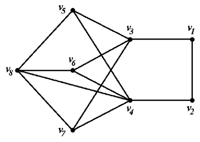
Figure 1: The Lemke graph

1.2 Results

The main tool we develop is the Weight Function Lemma 2. This lemma allows us to define a (very large) integer linear optimization problem that yields an upper bound on the pebbling number. This has several important consequences, including the following.

1. The pebbling numbers of reasonably small graphs often can be computed easily. Moreover, it is frequently the case that the fractional relaxation suffices for the task, allowing the computation for somewhat larger graphs.

2. It is also common that only a small portion of the constraints are required, expanding the pool of computable graphs even more. One can restrict the types of constraints to greedy, bounded depth, and so on, with great success, seemingly because of the comments above. Potentially, this allows one to begin to catalog special classes of graphs such as Class 0, (semi-)greedy, and tree-solvable.

3. The dual solutions often yield very short certificates of the results, in most cases quadratic in the number of vertices, and usually at most the number of vertices times the degree of the root. These certificates are remarkably simple compared to the usual solvability arguments that chase pebbles all over the graph in a barrage of cases. One can sometimes find such certificates for infinite families of graphs by hand, without resorting to machine for more than the smallest one or two of its members. This was our approach in Section 3.3, for example.

4. Our method gives trivial proofs of

   1. $\pi(C_{2k})=2^{k}$ and $\pi(C_{2k+1})=2\lfloor 2^{k+1}/3\rfloor+1$, which we write as $\lceil(2^{k+2}-1)/3\rceil$, and

   2. $C_{n}^{(k)}$ is Class 0 for $k\geq n/2(\lg n-\lg\lg n)$, where $G^{(k)}$ denotes the $k^{\rm th}$ graph power of $G$ (as opposed to the Cartesian power $G^{k}$). This answers a question of [20], who defined the pebbling exponent of $G$ minimum such $e=e_{\pi}(G)$ for which $\pi(G^{(e)})=n(G)$. Thus $e_{\pi}(G)\leq n/2(\lg n-\lg\lg n)$ (see Theorem 16), which is fairly close to the obvious lower bound of $n/2\lg n$.

In this paper we apply the Weight Function Lemma to several specific graphs, including the Petersen, Lemke, $4^{\rm th}$ weak Bruhat, Lemke squared, and two random graphs, as well as to a number of infinite families of graphs, such as trees, cycles, graph powers of cycles, cubes, and some generalized Petersen and Coxeter graphs.

2 The Weight Function Lemma

Let $P_{n}$ be the path $v_{1}v_{2}\cdots v_{n}$ on $n$ vertices. Then $\pi(P_{n})=2^{n-1}$ is easily proved by induction. In particular, any configuration of at least $2^{n-1}$ pebbles solves $v_{1}$. But one can say more about smaller $v_{1}$-solvable configurations as well, with the use of a weight function $w$. Define $w$ on $V(G)$ by $w(v_{n-i})=2^{i}$, and extend the weight function to configurations by $w(C)=\sum_{v\in V}w(v)C(v)$. Then a pebbling step can only preserve or decrease the weight of a configuration. Since the weight of a configuration with a pebble on $v_{1}$ is at least $2^{n-1}$, we see that $2^{n-1}$ is a lower bound on every $v_{1}$-solvable configuration. In fact, induction shows that every $v_{1}$-unsolvable configuration has weight at most $2^{n-1}-1$, which equals $\sum_{i=2}^{n}w(v_{i})$. That is, this inequality characterizes $v_{1}$-unsolvable configurations on $P_{n}$. The Weight Function Lemma 2 generalizes this result on trees, and we explore the applications of the lemma in the following sections.

2.1 Linear Optimization

Let $G$ be a graph and $T$ be a subtree of $G$ rooted at vertex $r$, with at least two vertices. For a vertex $v\in V(T)$ let $v^{+}$ denote the parent of $v$; i.e. the $T$-neighbor of $v$ that is one step closer to $r$ (we also say that $v$ is a child of $v^{+}$). We call $T$ a strategy when we associate with it a nonnegative, nonzero weight function $w$ with the property that $w(r)=0$ and $w(v^{+})=2w(v)$ for every other vertex that is not a neighbor of $r$ (and $w(v)=0$ for vertices not in $T$). Let ${\mathbf{T}}$ be the configuration with ${\mathbf{T}}(r)=0$, ${\mathbf{T}}(v)=1$ for all $v\in V(T)$, and ${\mathbf{T}}(v)=0$ everywhere else. With this notation note that the path result above can be restated: $C$ is $v_{1}$-unsolvable if and only if $C(v_{1})=0$ and $w(C)\leq w({\mathbf{T}})$, where $T$ is the strategy $T=P_{n}$ with associated weight function $w$.

Lemma 2

[Weight Function Lemma] Let $T$ be a strategy of $G$ rooted at $r$, with associated weight function $w$. Suppose that $C$ is an $r$-unsolvable configuration of pebbles on $V(G)$. Then $w(C)\leq w({\mathbf{T}})$.

Proof.  By contrapositive and induction. The base case is when $T$ is a path, which is proved above. Suppose $w(C)>w({\mathbf{T}})$, let $y$ be a leaf of $T$, and define $P$ to be the path from $y$ to $r$ in $T$, with $P_{y}$ being the subpath from $y$ to its closest vertex $x$ on $P$ of degree at least 3 in $T$ (or $r$ if none exists). Denote by $T^{\prime}$ the tree $T-P_{y}+x$, and among all such $r$-unsolvable configurations, choose $C$ to be the one having largest weight on $T^{\prime}$. The restriction $w^{\prime}$ of $w$ to $T^{\prime}$ witnesses that $T^{\prime}$ is a strategy for the root $r$, so induction requires that $w^{\prime}(C)\leq w^{\prime}({\mathbf{T}}^{\prime})$. Likewise, the restriction $w_{y}$ of $w$ to $P_{y}$ witnesses that $P_{y}$ is a strategy for the root $x$. Because $w(C)=w^{\prime}(C)+w_{y}(C)$ and $w({\mathbf{T}})=w^{\prime}({\mathbf{T}}^{\prime})+w_{y}(P_{y})$, we must have $w_{y}(C)>w_{y}(P_{y})$ which by induction means that the restriction of $C$ to $P_{y}-x$ solves $x$ (and so $x\not=r$). Let $C_{x}$ be the resulting configuration after moving a pebble from $P_{y}-x$ to $x$. Since $C$ is $r$-unsolvable, so is $C_{x}$. Now $w(C_{x})=w(C)$, but $w^{\prime}(C_{x})>w^{\prime}(C)$, which contradicts the initial choice of $C$. $\Box$

For a graph $G$ and root vertex $r$, let ${\cal T}$ be the set of all $r$-strategies in $G$, and denote by $z_{G,r}$ the optimal value of the integer linear optimization problem ${\mathbf{P}}_{G,r}$:

$${\rm Max.}\ \sum_{v\not=r}C(v)\ {\rm s.t.}\ w(C)\leq w({\mathbf{T}}),\ {\rm and\ }{\mathbf{T}}\in{\cal T}\ {\rm with\ witnessing\ weight\ function\ }w\ .$$ (1)

We also let $\hat{z}_{G,r}$ be the optimum of the relaxation, which allows configurations to be rational. We will find the relation $z_{G,r}\leq\lfloor\hat{z}_{G,r}\rfloor$ useful at times. The following corollary is straightforward.

Corollary 3

Every graph $G$ and root $r$ satisfies $\pi(G,r)\leq z_{G,r}+1$.

Proof.  By definition, the pebbling number is one more than the size of the largest unsolvable configuration. $\Box$

Until now, one could only use trees in an individual manner: $\pi(G,r)\leq\pi(T,r)$ for every spanning tree $T$ rooted at $r$. The Weight Function Lemma allows one to consider all subtrees rooted at $r$ (not only spanning trees) simultaneously, which we will see is significantly more powerful. One strength of the method is that the relaxation frequently has an integer optimum. This means that the dual solution will point out which tree constraints certify the result, and because the dual problem has only $n(G)-1$ constraints there are at most that many such trees in the certificate. Experience has shown, however, that usually one can find a certificate with only ${\sf deg}(r)$ trees (or sometimes a few extra). We will see this behavior starting in Section 3.

2.2 Basic Applications

We begin with the pebbling number of trees, whose formula was first discovered and proved in [7]. View a tree $T$ with root $r$ as a directed graph with every edge directed toward $r$. Then a path partition ${\cal P}$ of $T$ is a set of edge-disjoint directed paths whose union is $T$. One path partition majorizes another if its nonincreasing sequence of path lengths majorizes that of the other. A path partition is maximum if it majorizes all others. We can use Corollary 3 to give a new proof of the following result of [7].

Theorem 4

For a tree $T$ and root $r$ we have $\pi(T,r)=\sum_{P\in{\cal P}}2^{e_{P}}-|{\cal P}|+1$, where $e_{P}$ denotes the length (number of edges) of $P$.

Proof.  We begin by showing that a maximum size $r$-unsolvable configuration has pebbles on leaves only, and in fact on all leaves. Indeed, if $C$ has a pebble on the nonleaf $x$, then we define a pushback of $C$ at $x$ to be any configuration obtained by removing the $C(x)$ pebbles from $x$, adding $2C(x)+1$ pebbles to one of the children of $x$, and adding $1$ pebble to all other children of $x$. Certainly, if $C$ is $r$-unsolvable and has no pebbles past $x$ (on the subtree of $T$ rooted at $x$, minus $x$ itself), then the pushback will also be $r$-unsolvable, and thus satisfy the constraints of ${\mathbf{P}}_{T,r}$. It will also be larger than $C$. The configuration $C^{*}$ that places $2^{e_{P}}-1$ pebbles on the leaf of the path $P\in{\cal P}$ is one possible result of pushing back the empty configuration, and so satisfies the constraints of ${\mathbf{P}}_{T,r}$. Hence $\pi(T,r)\geq\sum_{P\in{\cal P}}2^{e_{P}}-|{\cal P}|+1$.

For the upper bound we prove that $C^{*}$ is optimal by using induction to show that the optimal configuration has $2^{e_{P}}-1$ pebbles on the leaf $y_{P}$ of $P$ for every $P\in{\cal P}$. This is true if $|{\cal P}|=1$, so suppose $|{\cal P}|\geq 2$ and let $Q$ denote one of the paths in ${\cal P}$ whose leaf has the highest weight in $w$, with a tie going to one of the shortest length. This is to guarantee that the graph $T-Q+x$, where $x$ is the root of $Q$, is a tree (i.e. is connected). In order to maximize the number of pebbles that satisfy $\sum_{P\in{\cal P}}w(y_{P})C(y_{P})\leq\sum_{P\in{\cal P}}w(P)$ we would transfer as many pebbles from $y_{Q}$ to other leaves as possible because their weights are at most $w(y_{P})$ and we could add extra pebbles when the weight is smaller. But by induction on $T-Q+x$ we know from the constraint $\sum_{P\in{\cal P}-\{Q\}}w(y_{P})C(y_{P})\leq\sum_{P\in{\cal P}-\{Q\}}w(P)$ that each $C(y_{P})\leq 2^{e_{P}}-1$, with equality for all $P\not=Q$ if and only if $C$ is maximum. Therefore, since $w(P)=w(y_{P})(2^{e_{P}}-1)$ for all $P\in{\cal P}$, we have

$$w(y_{P})C(y_{P}) \leq \sum_{P\in{\cal P}}w(P)-\sum_{P\in{\cal P}-\{Q\}}w(y_{P})(2^{e_{P}}-1)$$

$$= w(Q)$$

$$= w(y_{Q})(2^{e_{Q}}-1)\ ,$$

which implies that $C(y_{P})\leq 2^{e_{Q}}-1$. $\Box$

A slight weakness of these tree constraints is that they do not classify unsolvable configurations on trees the way that they do on paths. This is because they let in a few solvable configurations. For example, consider the star on four vertices with one of its leaves as root $r$. Then the configuration with $2$ pebbles on each of the other two leaves is $r$-solvable and satisfies all tree contraints. Since it is the average of the two $r$-unsolvable configurations that place either $1$ and $3$ or $3$ and $1$ on those other leaves, it cannot be cut out by the tree constraints that don’t cut out at least one of these two other constraints. In this case it doesn’t hurt us, since the strategy bound yields $\pi\leq 5$ and the actual pebbling number is 5, but it can cause trouble on graphs in general. For example, we know that the 3-cube $Q^{3}$ in Figure 2 has pebbling number 8, so that the shown configuration $C$ is solvable (pebbles from to top must be split in two directions in its solution). However, no strategy recognizes its solution, and Corollary 3 yields only $\pi(Q^{3})\leq 9$ (the three rotations of the strategy in the center in Figure 2 certify this). One can see where the aforementioned star appears in the Figure 2 configuration on $Q^{3}$ and is exploited accordingly: moving pebbles from the $5$ along one edge yields a $(3,1)$ configuration, while splitting the moves along two edges yields a $(2,2)$ configuration.

             

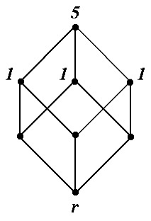
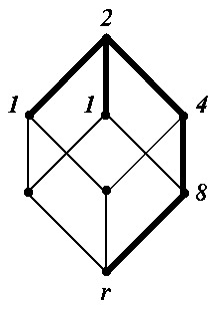
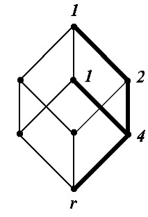
Figure 2: A solvable configuration (left) not recognized by any tree strategy; a canonical strategy (center) used for certifying $\pi(Q^{3})\leq 9$; a simplified nonbasic strategy (right) that does the same

3 General Applications

In this section we illustrate the method more fully by presenting short proofs of both known and new results. We begin by relaxing strategies in the following way. We now use the term basic to describe the strategies as currently defined. A nonbasic strategy will satisfy the inequality $w(v^{+})\geq 2w(v)$ in place of the equality used in a basic strategy (see Figure 2). The following lemma shows that we can use nonbasic strategies in an upper bound certificate since they are conic combinations of a nested family of basic strategies. Thus the use of nonbasic strategies can simplify and shorten certificates significantly.

Lemma 5

If $T$ is a nonbasic strategy for the rooted graph $(G,r)$, then there exists basic strategies $T_{1},\ldots,T_{k}$ for $(G,r)$ and nonnegative constants $c_{1},\ldots,c_{k}$ so that $T=\sum_{i=1}^{k}c_{i}T_{i}$.

Proof.  We use induction, as the result is true when $T$ has two vertices since $T$ is basic then. Given $T$, let $S$ be a basic strategy on the edge set of $T$, define $c$ to be the largest constant for which $cS\leq T$, and denote $T^{\prime}=T-cS$. Then some vertex $v$ of $G$ satisfies $cS(v)=T(v)$, so $T^{\prime}$ has fewer vertices than $T$. Also, because $S$ is basic, any vertex $u$ whose unique $ur$-path contains $v$ also satisfies $cS(u)=T(u)$, which means that $T^{\prime}$ is connected, and hence a strategy. Moreover, $T^{\prime}$ is nonbasic since every nonneighbor $x$ of $r$ has $T^{\prime}(x^{+})=T(x^{+})-cS(x^{+})\geq 2T(x)-2cS(x)=2T^{\prime}(x)$. By induction, $T^{\prime}$ is a conic combination of basic strategies, and so therefore is $T$. $\Box$

We use conic combinations of strategies to derive, for some ${\alpha}$, the inequality $|C|=\sum_{v\not=r}C(v)\leq{\alpha}$ for $r$-unsolvable configurations $C$. From this we surmise that $\pi(G)\leq\lfloor{\alpha}\rfloor+1$. Instead of writing our strategies algebraically, it will be somewhat easier to show them graphically. We will display them so as to derive $m\sum_{v\not=r}C(v)\leq\sum_{v\not=r}m_{v}C(v)\leq m{\alpha}$ for some sequence $\{m_{v}\}_{v}$ with $m=\min_{v}m_{v}$, and let the reader divide by $m$. In fact, in many instances we will derive $m_{v}=m$ for all $v\not=r$, which makes for the following observation.

Lemma 6

[Uniform Covering Lemma] Let ${\cal T}$ be a set of strategies for the root $r$ of the graph $G$. If there is some $m$ such that, for each vertex $v\not=r$, we have $\sum_{T\in{\cal T}}T(v)=m$, then $\pi(G,r)=n(G)$. $\Box$

3.1 Specific Graphs

It has been said in jest that every graph theory paper should contain the Petersen graph, so we get it out of the way first.

Theorem 7

Let $P$ denote the Petersen graph. Then $\pi(P)\leq 10$.

Of course, the vertex lower bound implies $\pi(P)=10$, but since the focus of this paper regards upper bounds, we prove them only.

Proof.  The $3$ strategies shown in Figure 3 certify the result. $\Box$

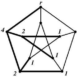
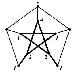
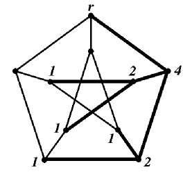
Figure 3: Petersen Class 0 certificate

Without such nice symmetry, the Lemke graph requires a different certificate for each possible root.

Theorem 8

Let $L$ denote the Lemke graph and suppose $r\not=v_{1}$. Then $\pi(L,r)\leq 8$.

Proof.  We show the strategies for each root vertex in turn, below.

For $r=v_{2}$:

For $r=v_{3}$:

Without the edge $v_{4}v_{8}$, the resulting graph would view $v_{3}$ and $v_{4}$ symmetrically. Using that symmetry, the solutions for $r=v_{3}$ become solutions for $v_{4}$.

For $r=v_{5}$:

      

For $r\in\{v_{6},v_{7}\}$ we use the solutions from the case $r=v_{5}$ given by the appropriate symmetry.

For $r=v_{8}$:

      

                         

$\Box$

Because of the $3$-cube-like configuration with $(1,1,1,5)$ on $(v_{5},v_{6},v_{7},v_{8})$, the best that our tree strategies can muster is $\pi(L,v_{1})\leq 9$. Thus, to show that $L$ is Class 0 one must handle $v_{1}$ by more traditional methods.

To illustrate that larger graphs can be tackled, we move on to one of order 24 that is not Class 0. Define the (weak) Bruhat graph of order $m$ (see Figure 4) to have all permutations of $[m]$ as vertices, with an edge between pairs of permutations that differ by an adjacent transposition. One can recognize it as the Cayley graph of $S_{m}$, generated by adjacent transpositions, and also note that $B_{4}$ is the cubic Ramanujan (expander) graph of [6]. Intuitively, expander graphs would seem to have low pebbling numbers, but because $B_{4}$ has diameter 6 we have the lower bound $\pi(B_{4})\geq 64$. We give here a fairly tight bound.

Theorem 9

Let $B_{4}$ be the Bruhat graph of order 4. Then $\pi(B_{4})\leq 72$.

Proof.  Because the graph is vertex transitive, only one root must be checked. The $3$ strategies shown in Figure 4 certify the result. We combined them into one figure, separated by edge styles. $\Box$

      

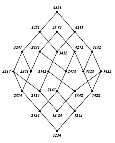
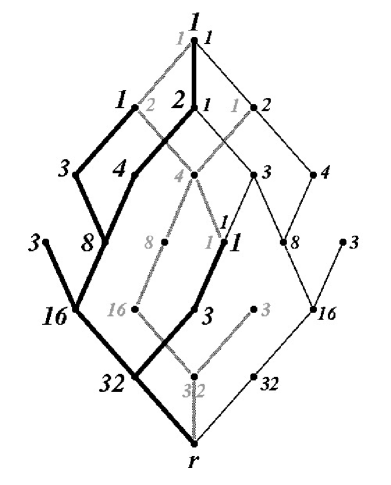
Figure 4: Bruhat graph $B_{4}$ (left) and strategies (right)

Next we consider ${L{\mathchoice{\vbox{\hrule height=0.4pt\hbox{\vrule width=0.4pt,height=3.0pt\kern 3.0pt\vrule width=0.4pt} \hrule height=0.4pt}}{\vbox{\hrule height=0.4pt\hbox{\vrule width=0.4pt,height=3.0pt\kern 3.0pt\vrule width=0.4pt} \hrule height=0.4pt}}{\vbox{\hrule height=0.3pt\hbox{\vrule width=0.3pt,height=2.1pt\kern 2.1pt\vrule width=0.3pt} \hrule height=0.3pt}}{\vbox{\hrule height=0.3pt\hbox{\vrule width=0.3pt,height=1.5pt\kern 1.5pt\vrule width=0.3pt} \hrule height=0.3pt}}}L}$, the square of the Lemke graph $L$. Because $L$ has diameter 3, ${L{\mathchoice{\vbox{\hrule height=0.4pt\hbox{\vrule width=0.4pt,height=3.0pt\kern 3.0pt\vrule width=0.4pt} \hrule height=0.4pt}}{\vbox{\hrule height=0.4pt\hbox{\vrule width=0.4pt,height=3.0pt\kern 3.0pt\vrule width=0.4pt} \hrule height=0.4pt}}{\vbox{\hrule height=0.3pt\hbox{\vrule width=0.3pt,height=2.1pt\kern 2.1pt\vrule width=0.3pt} \hrule height=0.3pt}}{\vbox{\hrule height=0.3pt\hbox{\vrule width=0.3pt,height=1.5pt\kern 1.5pt\vrule width=0.3pt} \hrule height=0.3pt}}}L}$ has diameter 6, and so $\pi({L{\mathchoice{\vbox{\hrule height=0.4pt\hbox{\vrule width=0.4pt,height=3.0pt\kern 3.0pt\vrule width=0.4pt} \hrule height=0.4pt}}{\vbox{\hrule height=0.4pt\hbox{\vrule width=0.4pt,height=3.0pt\kern 3.0pt\vrule width=0.4pt} \hrule height=0.4pt}}{\vbox{\hrule height=0.3pt\hbox{\vrule width=0.3pt,height=2.1pt\kern 2.1pt\vrule width=0.3pt} \hrule height=0.3pt}}{\vbox{\hrule height=0.3pt\hbox{\vrule width=0.3pt,height=1.5pt\kern 1.5pt\vrule width=0.3pt} \hrule height=0.3pt}}}L})\geq 64$. Strategies deliver the following upper bounds. Since the bounds are not that tight, we do not pursue bounds for all $64$ vertices, although it is likely (since $v_{1}$ is the most problematic root in $L$) that the upper bound of $108$ works for all roots $(r_{1},r_{2})$.

Theorem 10

Let ${L{\mathchoice{\vbox{\hrule height=0.4pt\hbox{\vrule width=0.4pt,height=3.0pt\kern 3.0pt\vrule width=0.4pt} \hrule height=0.4pt}}{\vbox{\hrule height=0.4pt\hbox{\vrule width=0.4pt,height=3.0pt\kern 3.0pt\vrule width=0.4pt} \hrule height=0.4pt}}{\vbox{\hrule height=0.3pt\hbox{\vrule width=0.3pt,height=2.1pt\kern 2.1pt\vrule width=0.3pt} \hrule height=0.3pt}}{\vbox{\hrule height=0.3pt\hbox{\vrule width=0.3pt,height=1.5pt\kern 1.5pt\vrule width=0.3pt} \hrule height=0.3pt}}}L}$ be the square of the Lemke graph $L$. Then

$$\pi({L{\mathchoice{\vbox{\hrule height=0.4pt\hbox{\vrule width=0.4pt,height=3.0pt\kern 3.0pt\vrule width=0.4pt} \hrule height=0.4pt}}{\vbox{\hrule height=0.4pt\hbox{\vrule width=0.4pt,height=3.0pt\kern 3.0pt\vrule width=0.4pt} \hrule height=0.4pt}}{\vbox{\hrule height=0.3pt\hbox{\vrule width=0.3pt,height=2.1pt\kern 2.1pt\vrule width=0.3pt} \hrule height=0.3pt}}{\vbox{\hrule height=0.3pt\hbox{\vrule width=0.3pt,height=1.5pt\kern 1.5pt\vrule width=0.3pt} \hrule height=0.3pt}}}L},(r,r))\leq\Bigg{\{}\begin{array}[]{rcl}108&&{\rm if\ }r=v_{1}\ ,\\ 96&&{\rm if\ }r=v_{8}{\rm\ ,\ and}\\ 68&&{\rm if\ }r=v_{4}\ .\end{array}$$

Proof.  For $r=v_{1}$ one can verify that a quarter of the sum of the four strategies in Figure 5 yields the weights

$$\qquad\begin{array}[]{c|c|c|c|c|c|c|c|c|}T_{3}&v_{1}&v_{2}&v_{3}&v_{4}&v_{5}&v_{6}&v_{7}&v_{8}\\ \hline\cr v_{1}&0&8&8&1&4&1&1&2\\ \hline\cr v_{2}&8&4&1&2&1&1&1&1\\ \hline\cr v_{3}&8&4&1&1&1&1&1&1\\ \hline\cr v_{4}&4&1&1&1&1&1&1&1\\ \hline\cr v_{5}&1&2&1&1&1&1&1&1\\ \hline\cr v_{6}&1&1&1&1&1&1&1&1\\ \hline\cr v_{7}&1&1&1&1&1&1&1&1\\ \hline\cr v_{8}&2&1&1&1&1&1&1&1\\ \hline\cr\end{array}\ ,$$

giving the bound of $63+4(7+3+1)+1=108$. One verifies that each $T_{i}$ is a strategy by making sure that each nonzero entry has a corresponding entry in its column or row with at least twice its weight that is joined to it by an edge in the appropriate copy of $L$.

$$\begin{array}[]{c|c|c|c|c|c|c|c|c|}T_{1}&v_{1}&v_{2}&v_{3}&v_{4}&v_{5}&v_{6}&v_{7}&v_{8}\\ \hline\cr v_{1}&0&&32&&16&4&4&8\\ \hline\cr v_{2}&&&4&&&&&\\ \hline\cr v_{3}&&&4&&2&2&2&4\\ \hline\cr v_{4}&&&&&&&&\\ \hline\cr v_{5}&&&2&&1&1&1&2\\ \hline\cr v_{6}&&&2&&1&1&1&\\ \hline\cr v_{7}&&&2&&1&1&1&\\ \hline\cr v_{8}&&&&&&&&1\\ \hline\cr\end{array}\qquad\begin{array}[]{c|c|c|c|c|c|c|c|c|}T_{2}&v_{1}&v_{2}&v_{3}&v_{4}&v_{5}&v_{6}&v_{7}&v_{8}\\ \hline\cr v_{1}&0&&&&&&&\\ \hline\cr v_{2}&32&&&&&&&\\ \hline\cr v_{3}&&&&&&&&\\ \hline\cr v_{4}&16&4&4&&2&2&2&2\\ \hline\cr v_{5}&4&&2&&1&1&1&\\ \hline\cr v_{6}&4&&2&&1&1&1&2\\ \hline\cr v_{7}&4&&2&&1&1&1&2\\ \hline\cr v_{8}&8&&4&&2&2&2&1\\ \hline\cr\end{array}$$

$$\begin{array}[]{c|c|c|c|c|c|c|c|c|}T_{3}&v_{1}&v_{2}&v_{3}&v_{4}&v_{5}&v_{6}&v_{7}&v_{8}\\ \hline\cr v_{1}&0&&&&&&&\\ \hline\cr v_{2}&&&&&&&&\\ \hline\cr v_{3}&32&16&&4&2&2&2&\\ \hline\cr v_{4}&&&&&&&&\\ \hline\cr v_{5}&&8&&2&1&1&1&1\\ \hline\cr v_{6}&&4&&2&1&1&1&1\\ \hline\cr v_{7}&&4&&2&1&1&1&1\\ \hline\cr v_{8}&&4&&2&1&1&1&1\\ \hline\cr\end{array}\qquad\begin{array}[]{c|c|c|c|c|c|c|c|c|}T_{4}&v_{1}&v_{2}&v_{3}&v_{4}&v_{5}&v_{6}&v_{7}&v_{8}\\ \hline\cr v_{1}&0&32&&4&&&&\\ \hline\cr v_{2}&&16&&8&4&4&4&4\\ \hline\cr v_{3}&&&&&&&&\\ \hline\cr v_{4}&&&&4&2&2&2&2\\ \hline\cr v_{5}&&&&2&1&1&1&1\\ \hline\cr v_{6}&&&&2&1&1&1&1\\ \hline\cr v_{7}&&&&2&1&1&1&1\\ \hline\cr v_{8}&&&&2&1&1&1&1\\ \hline\cr\end{array}$$

Figure 5: Strategies for ${L{\mathchoice{\vbox{\hrule height=0.4pt\hbox{\vrule width=0.4pt,height=3.0pt\kern 3.0pt\vrule width=0.4pt} \hrule height=0.4pt}}{\vbox{\hrule height=0.4pt\hbox{\vrule width=0.4pt,height=3.0pt\kern 3.0pt\vrule width=0.4pt} \hrule height=0.4pt}}{\vbox{\hrule height=0.3pt\hbox{\vrule width=0.3pt,height=2.1pt\kern 2.1pt\vrule width=0.3pt} \hrule height=0.3pt}}{\vbox{\hrule height=0.3pt\hbox{\vrule width=0.3pt,height=1.5pt\kern 1.5pt\vrule width=0.3pt} \hrule height=0.3pt}}}L}$ at $(v_{1},v_{1})$.

We use a similar argument when $r=v_{8}$, using the strategies from Figure 6, along with their transposes, and divide by 8 to obtain the bound $63+8(3+1)+1=96$.

$$\begin{array}[]{c|c|c|c|c|c|c|c|c|}T_{1}&v_{1}&v_{2}&v_{3}&v_{4}&v_{5}&v_{6}&v_{7}&v_{8}\\ \hline\cr v_{1}&1&2&2&4&4&4&4&8\\ \hline\cr v_{2}&&&&&&&&\\ \hline\cr v_{3}&&&&&&8&8&16\\ \hline\cr v_{4}&&&&&&&&\\ \hline\cr v_{5}&&&&&&&&\\ \hline\cr v_{6}&&&&&&&&\\ \hline\cr v_{7}&&&&8&8&8&4&32\\ \hline\cr v_{8}&&&&&&&&0\\ \hline\cr\end{array}\qquad\begin{array}[]{c|c|c|c|c|c|c|c|c|}T_{2}&v_{1}&v_{2}&v_{3}&v_{4}&v_{5}&v_{6}&v_{7}&v_{8}\\ \hline\cr v_{1}&1&2&2&4&4&4&4&\\ \hline\cr v_{2}&2&4&4&8&8&8&8&16\\ \hline\cr v_{3}&&&&&&&&\\ \hline\cr v_{4}&&&&&&&&32\\ \hline\cr v_{5}&&&&&&&&\\ \hline\cr v_{6}&&&&&&&&\\ \hline\cr v_{7}&&&&&&&&\\ \hline\cr v_{8}&&&&&&&&0\\ \hline\cr\end{array}$$

$$\begin{array}[]{c|c|c|c|c|c|c|c|c|}T_{3}&v_{1}&v_{2}&v_{3}&v_{4}&v_{5}&v_{6}&v_{7}&v_{8}\\ \hline\cr v_{1}&1&2&&&&&&\\ \hline\cr v_{2}&&&&&&&&\\ \hline\cr v_{3}&&4&&8&&&&\\ \hline\cr v_{4}&&&&4&&&&\\ \hline\cr v_{5}&&&&16&4&&8&32\\ \hline\cr v_{6}&&&&&&&&\\ \hline\cr v_{7}&&&&&&&&\\ \hline\cr v_{8}&&&&&&&&0\\ \hline\cr\end{array}\qquad\begin{array}[]{c|c|c|c|c|c|c|c|c|}T_{4}&v_{1}&v_{2}&v_{3}&v_{4}&v_{5}&v_{6}&v_{7}&v_{8}\\ \hline\cr v_{1}&1&&2&&&&&\\ \hline\cr v_{2}&&&&&&&&\\ \hline\cr v_{3}&2&&4&&8&&&\\ \hline\cr v_{4}&&&&&&&&\\ \hline\cr v_{5}&&&&&&&&\\ \hline\cr v_{6}&&&&8&16&4&&32\\ \hline\cr v_{7}&&&&&&&&\\ \hline\cr v_{8}&&&&&&&&0\\ \hline\cr\end{array}$$

Figure 6: Strategies for ${L{\mathchoice{\vbox{\hrule height=0.4pt\hbox{\vrule width=0.4pt,height=3.0pt\kern 3.0pt\vrule width=0.4pt} \hrule height=0.4pt}}{\vbox{\hrule height=0.4pt\hbox{\vrule width=0.4pt,height=3.0pt\kern 3.0pt\vrule width=0.4pt} \hrule height=0.4pt}}{\vbox{\hrule height=0.3pt\hbox{\vrule width=0.3pt,height=2.1pt\kern 2.1pt\vrule width=0.3pt} \hrule height=0.3pt}}{\vbox{\hrule height=0.3pt\hbox{\vrule width=0.3pt,height=1.5pt\kern 1.5pt\vrule width=0.3pt} \hrule height=0.3pt}}}L}$ at $(v_{8},v_{8})$.

Likewise, for $r=v_{4}$, the strategies and their transposes from Figure 7 yield an upper bound of $63+\lfloor 8(.6)\rfloor+1=68$. $\Box$

$$\begin{array}[]{c|c|c|c|c|c|c|c|c|}T_{1}&v_{4}&v_{8}&v_{7}&v_{6}&v_{5}&v_{2}&v_{3}&v_{1}\\ \hline\cr v_{4}&0&&&&&&&\\ \hline\cr v_{8}&10&5&4&2&4&4&2&\\ \hline\cr v_{7}&&&&&&&&\\ \hline\cr v_{6}&&&&&&&&\\ \hline\cr v_{5}&&&&&&&&\\ \hline\cr v_{2}&&&&&&&&\\ \hline\cr v_{3}&&&&&&&&\\ \hline\cr v_{1}&&&&&&&&\\ \hline\cr\end{array}\qquad\begin{array}[]{c|c|c|c|c|c|c|c|c|}T_{2}&v_{4}&v_{8}&v_{7}&v_{6}&v_{5}&v_{2}&v_{3}&v_{1}\\ \hline\cr v_{4}&0&&&&&&&\\ \hline\cr v_{8}&&&&&&&&\\ \hline\cr v_{7}&16&6&5&2&8&8&2&4\\ \hline\cr v_{6}&&&&&&&&\\ \hline\cr v_{5}&&&&&&&&\\ \hline\cr v_{2}&&&&&&&&\\ \hline\cr v_{3}&8&4&4&4&4&4&2&1\\ \hline\cr v_{1}&2&2&&2&2&2&1&1\\ \hline\cr\end{array}$$

$$\begin{array}[]{c|c|c|c|c|c|c|c|c|}T_{3}&v_{4}&v_{8}&v_{7}&v_{6}&v_{5}&v_{2}&v_{3}&v_{1}\\ \hline\cr v_{4}&0&&&&&&&\\ \hline\cr v_{8}&&&&&&&&\\ \hline\cr v_{7}&&&&&&&&\\ \hline\cr v_{6}&16&8&8&5&8&8&2&4\\ \hline\cr v_{5}&&&&&&&&\\ \hline\cr v_{2}&&&&&&&&\\ \hline\cr v_{3}&2&4&4&2&4&4&2&2\\ \hline\cr v_{1}&&2&2&&2&2&1&1\\ \hline\cr\end{array}\qquad\begin{array}[]{c|c|c|c|c|c|c|c|c|}T_{4}&v_{4}&v_{8}&v_{7}&v_{6}&v_{5}&v_{2}&v_{3}&v_{1}\\ \hline\cr v_{4}&0&&&&&&&\\ \hline\cr v_{8}&&&&&&&&\\ \hline\cr v_{7}&&&&&&&&\\ \hline\cr v_{6}&&&&&&&&\\ \hline\cr v_{5}&16&6&2&2&5&8&2&4\\ \hline\cr v_{2}&&&&&&&&\\ \hline\cr v_{3}&&&&&&2&1&2\\ \hline\cr v_{1}&&&&&&&&1\\ \hline\cr\end{array}$$

$$\begin{array}[]{c|c|c|c|c|c|c|c|c|}T_{5}&v_{4}&v_{8}&v_{7}&v_{6}&v_{5}&v_{2}&v_{3}&v_{1}\\ \hline\cr v_{4}&0&&&&&&&\\ \hline\cr v_{8}&&&&&&&&\\ \hline\cr v_{7}&&&&&&&&\\ \hline\cr v_{6}&&&&&&&&\\ \hline\cr v_{5}&&&&&&&&\\ \hline\cr v_{2}&16&6&2&2&2&5&&2\\ \hline\cr v_{3}&&&&2&&&&\\ \hline\cr v_{1}&8&4&4&4&2&4&2&2\\ \hline\cr\end{array}$$

Figure 7: Strategies for ${L{\mathchoice{\vbox{\hrule height=0.4pt\hbox{\vrule width=0.4pt,height=3.0pt\kern 3.0pt\vrule width=0.4pt} \hrule height=0.4pt}}{\vbox{\hrule height=0.4pt\hbox{\vrule width=0.4pt,height=3.0pt\kern 3.0pt\vrule width=0.4pt} \hrule height=0.4pt}}{\vbox{\hrule height=0.3pt\hbox{\vrule width=0.3pt,height=2.1pt\kern 2.1pt\vrule width=0.3pt} \hrule height=0.3pt}}{\vbox{\hrule height=0.3pt\hbox{\vrule width=0.3pt,height=1.5pt\kern 1.5pt\vrule width=0.3pt} \hrule height=0.3pt}}}L}$ at $(v_{4},v_{4})$.

One can see where the improvement from 108 to 96 comes from. We obtain a bound from a sum of strategies by dividing by the minimum weight, and since the graph has diameter six, the maximum weight is at least 32. So we need to increase the minimum weight as much as possible by including more strategies, but there are diminishing returns. In the case of root $(v_{1},v_{1})$, it has four neighbors, and so a fifth strategy increases the maximum weight to at least 64. This is why the root $(v_{8},v_{8})$, having eight neighbors, fares better. On this basis one might expect the root $(v_{4},v_{4})$ to perform best. In fact, it does even better for a different reason: it has eccentricity $4$. It is amusing that the order of this graph is out of the range of computing, while these strategies were found fairly easily by hand.

3.2 Random Graphs

Given our introductory comments and observations, we also tested some modest sized random graphs. Let $R_{15}$ denote the $15$-vertex graph given by the adjacency list

$([2,4,5,6,12,13],[1,3,4,8,11,12,14],[2,4,6,7],[1,2,3,5,7,9,14],[1,4,6,8,11,15],$ $[1,3,5,9,13,14],[3,4,11,15],[2,5,10,13,14,15],[4,6,10,11],[8,9,11],$
$[2,5,7,9,10,12,15],[1,2,11,13],[1,6,8,12],[2,4,6,8],[5,7,8,11])$.

We generated this graph with edge probability $.35$. It has diameter three, with $10$ of the vertices (including $v_{9}$) having distance two from all others. We found that $R_{15}$ is at least nearly Class 0 as follows. Our simple certificate of 3 basic strategies for the root $r=v_{9}$ is below.

$$2x_{1}+2x_{2}+2x_{3}+4x_{4}+2x_{5}+2x_{7}+x_{8}+x_{12}+x_{13}+2x_{14}+x_{15} \leq 20$$

$$2x_{2}+2x_{7}+2x_{8}+4x_{10}+4x_{11}+2x_{12}+x_{13}+2x_{15} \leq 19$$

$$2x_{1}+2x_{3}+2x_{5}+4x_{6}+x_{8}+x_{12}+2x_{13}+2x_{14}+x_{15} \leq 17$$

We note that there are $20,422$ basic strategies of depth at most two rooted at $r$. These were generated by our java code in a few minutes on my Core 2 Duo 2.66GhZ PC, with 2GB RAM and 250GB HD running Ubuntu linux 9.04. CPLEX software solved the resulting linear optimization problem instantly, delivering a dual certificate of a conic combination of $11$ of the strategies. By hand, we grouped them according to their neighbor of $r$ and were able to combine each into a single nonbasic strategy. By trading weights between some of the strategies, we arrived at the simplified certificate above. The certificate might be more easily viewed in the table of coefficients, below, in which the sum of the constraints appears below the line. Thus $\pi(R_{15},v_{9})\leq 15$.

$$\left(\begin{array}[]{rrrrrrrrrrrrrrr|r}2&2&2&4&2&0&2&1&0&0&0&1&1&2&1&20\\ 0&2&0&0&0&0&2&2&0&4&4&2&1&0&2&19\\ 2&0&2&0&2&4&0&1&0&0&0&1&2&2&1&17\\ \hline\cr 4&4&4&4&4&4&4&4&0&4&4&4&4&4&4&56\\ \end{array}\right)$$

The same upper bound of 15 was obtained for all other roots (see the Appendix) except for $v_{10}$, for which we found $\pi(R_{15},v_{10})\leq 16$. Note that $R_{15}$ contains the $4$-cycle $(v_{4},v_{3},v_{6},v_{9})$, with $v_{9}$ adjacent to the root $v_{10}$ — the same dreaded configuration we discussed in $Q^{3}$ obstructs us here: $(1,5,1,0)$. More to the point, let $C$ be the size $15$ configuration $(1,$ $1,$ $5,$ $1,$ $1,$ $1,$ $1,$ $0,$ $0,$ $0,$ $0,$ $1,$ $1,$ $1,$ $1)$ on $R_{15}$. Because $v_{3}$ is distance $3$ from the root $v_{10}$ and $C$ is empty on the neighbors of $v_{10}$, the only way to move a pebble to the root involves splitting the pebbles from $v_{3}$ as in the dreaded configuration solution. Hence no strategy can detect the $v_{10}$-solvability of $C$. However, we can blend strategies with some case analysis and slight amount of old fashioned analysis as follows.

Theorem 11

The graph $R_{15}$ is Class 0.

Proof.  As we have already shown that $\pi(R_{15},r)=15$ for all $r$ except for $v_{10}$, it suffices to prove that $\pi(R_{15},v_{10})$. Let $C$ be an $r$-unsolvable configuration, where $r=v_{10}$. We first consider the case that $C$ contains a pebble on a neighbor of $r$. In this case we have $x_{8}+x_{9}+x_{11}\geq 1$, and the CPLEX certificate

$$\left(\begin{array}[]{r|rrrrrrrrrrrrrrr|r}333&0&0&0&0&0&0&0&-1&-1&0&-1&0&0&0&0&-1\\ 80&2&0&2&3&0&4&0&0&8&0&0&0&2&2&0&23\\ 37&2&0&2&4&2&4&0&0&8&0&0&0&1&2&0&25\\ 50&2&2&2&4&2&3&2&0&8&0&0&0&0&2&0&27\\ 3&2&4&2&2&0&1&0&8&0&0&0&2&4&4&0&29\\ 1&2&4&2&2&0&2&0&8&0&0&0&2&4&0&3&29\\ 136&2&1&2&2&4&0&4&0&0&0&8&4&2&0&2&31\\ 25&2&3&2&2&4&2&4&0&0&0&8&4&0&0&2&33\\ 4&2&4&2&2&3&0&0&0&0&0&8&4&2&0&4&31\\ 37&2&4&2&2&1&2&0&8&0&0&0&2&0&4&4&31\\ 127&2&4&2&0&1&2&2&8&0&0&0&2&4&4&4&35\\ 1&2&4&2&2&4&2&1&0&0&0&8&4&2&2&4&37\\ \hline\cr&1002&1003&1002&1002&998&1003&999&1011&1003&0&995&1000&1003&1004&1001&14692\\ \end{array}\right)$$

shows that $|C|\leq 14$. In this format, the left column holds the multipliers of each constraint, and the bottom row is the result of the linear combination of them. Division by $995$ yields the result.

Thus we may assume that $x_{8}+x_{9}+x_{11}=0$. Next we consider the case that at most $5$ pebbles are distance $3$ from $r$; that is, $x_{1}+x_{3}\leq 5$. Here we have the certificate

$$\left(\begin{array}[]{r|rrrrrrrrrrrrrrr|r}84&1&0&1&0&0&0&0&0&0&0&0&0&0&0&0&5\\ 168&0&0&0&0&0&0&0&1&1&0&1&0&0&0&0&0\\ 6&2&4&2&2&3&2&0&8&0&0&0&2&4&4&0&33\\ 13&2&0&2&4&0&4&1&0&8&0&0&0&2&2&0&25\\ 29&2&0&2&4&2&4&2&0&8&0&0&0&1&2&0&27\\ 55&2&4&2&2&0&2&2&8&0&0&0&2&3&4&4&35\\ 23&2&4&2&2&4&2&1&8&0&0&0&2&4&4&4&39\\ 42&2&0&2&2&4&2&4&0&0&0&8&4&2&0&1&31\\ 6&2&4&2&2&4&2&4&0&0&0&8&4&2&2&1&37\\ 36&2&4&2&2&4&2&3&0&0&0&8&4&2&2&4&39\\ \hline\cr&504&504&504&504&504&504&504&840&504&0&840&504&504&504&504&7476\\ \end{array}\right)\ .$$

On the other hand, at least $7$ pebbles at distance $3$ from $r$ yields the following certificate.

$$\left(\begin{array}[]{r|rrrrrrrrrrrrrrr|r}20&-1&0&-1&0&0&0&0&0&0&0&0&0&0&0&0&-7\\ 1&2&4&2&0&0&0&0&8&0&0&0&0&0&4&3&23\\ 5&2&0&2&4&1&0&0&0&8&0&0&0&0&0&0&17\\ 3&2&0&2&0&0&4&0&0&8&0&0&0&1&0&0&17\\ 2&2&0&2&0&1&4&0&0&8&0&0&0&0&2&0&19\\ 3&2&4&2&0&4&0&0&8&0&0&0&0&4&4&1&29\\ 1&2&4&2&0&1&0&0&8&0&0&0&0&0&0&4&21\\ 5&2&0&2&0&0&0&4&0&0&0&8&4&1&0&2&23\\ \hline\cr&20&20&20&20&20&20&20&40&80&0&40&20&20&20&20&280\\ \end{array}\right)$$

Hence we may also assume that $x_{1}+x_{3}=6$, and so there are exactly $9$ pebbles on the $9$ vertices at distance two from $r$ if we assume that $|C|=15$.

Now, $v_{1}$ and $v_{3}$ can both reach all neighbors of $r$, so if either $x_{1}\geq 4$ or $x_{3}\geq 4$ then we can place a pebble on any neighbor of $r$. This forces each vertex at distance two from $r$ to have at most, and hence exactly $1$ pebble. Thus the splitting of the 4 pebbles will place a pebble on $r$. This contradiction means that $x_{1}=x_{3}=3$.

Similarly, then, the pair of $v_{1}$ and $v_{3}$ can place a pebble on any neighbor of $r$ via a common neighbor, again forcing $1$ pebble on every vertex at distance two from $r$. However, this allows $v_{1}$ and $v_{3}$ to each place a pebble on the same neighbor of $r$ via disjoint paths.

This final contradiction shows $|C|\leq 14$ again, finishing the proof. $\Box$

Next we considered the random graph $R_{20}$ having adjacency list

$([6,8,11,12,14,15,16,17]$, $[4,5,6,7,8,10,15,16,17,18,19,20]$,
$[4,6,8,12,14,20]$, $[2,3,5,6,8,9,12,15,18,19]$, $[2,4,7,12,14,15,16,18,20]$,
$[1,2,3,4,7,8,14,15,19]$, $[2,5,6,8,11,12,13,14,15,17,18]$,
$[1,2,3,4,6,7,10,11,14,15,17]$, $[4,10,11,13,14,17,19,20]$,
$[2,8,9,16,18,19,20]$, $[1,7,8,9,13,14,16,18,20]$, $[1,3,4,5,7,13,16]$,
$[7,9,11,12,19,20]$, $[1,3,5,6,7,8,9,11,18]$, $[1,2,4,5,6,7,8,19]$,
$[1,2,5,10,11,12,18,20]$, $[1,2,7,8,9,19]$, $[2,4,5,7,10,11,14,16,20]$,
$[2,4,6,9,10,13,15,17,20]$, $[2,3,5,9,10,11,13,16,18,19])$,

generated with edge probability $.4$. The graph has diameter two, does not have the form of the Class 1 characterization, and so must be Class 0. Indeed, from the $9,371$ basic strategies of depth at most two for the root $r=v_{1}$ (other roots had between 8,000–28,000 such strategies), CPLEX delivered the following certificate involving 16 of them (which we won’t bother to simplify) in Figure 8.

$\left(\begin{array}[]{r|rrrrrrrrrrrrrrrrrrrr|r}1469&0&2&1&0&0&4&0&0&0&0&0&0&0&0&0&0&0&0&2&0&9\\ 623&0&0&0&2&0&4&0&0&0&0&0&0&0&0&1&0&0&0&2&0&9\\ 473&0&0&0&2&0&0&1&4&0&2&0&0&0&2&0&0&0&0&0&0&11\\ 191&0&0&2&1&0&2&2&4&0&2&0&0&0&0&2&0&0&0&0&0&15\\ 1308&0&0&2&2&0&0&1&4&0&2&0&0&0&0&0&0&2&0&0&0&13\\ 527&0&0&0&0&0&0&0&4&0&2&0&0&0&0&1&0&2&0&0&0&9\\ 488&0&0&0&0&0&0&0&0&0&0&4&0&2&2&0&0&0&1&0&2&11\\ 2012&0&0&0&0&0&0&0&0&2&0&4&0&2&1&0&0&0&2&0&2&13\\ 2500&0&0&2&2&2&0&1&0&0&0&0&4&2&0&0&0&0&0&0&0&13\\ 1250&0&0&0&0&2&1&0&0&2&0&0&0&0&4&0&0&0&0&0&0&9\\ 221&0&0&2&0&0&0&0&0&1&0&0&0&0&4&0&0&0&2&0&0&9\\ 45&0&0&2&0&0&0&0&0&2&0&0&0&0&4&0&0&0&1&0&0&9\\ 4234&0&0&0&0&0&0&1&0&0&0&0&0&0&0&2&0&0&0&1&0&4\\ 2500&0&2&0&0&1&0&0&0&0&2&0&0&0&0&0&4&0&2&0&2&13\\ 1031&0&2&0&0&0&0&0&0&2&0&0&0&0&0&0&0&4&0&1&0&9\\ 551&0&0&0&0&0&0&2&0&2&0&0&0&0&0&0&0&4&0&1&0&9\\ \hline\cr 0&0&10000&9999&9999&10000&10000&9999&9996&9999&9998&10000&10000&10000&9998&10000&10000&9998&9999&10000&10000&189985\\ \end{array}\right)$

Figure 8: Certificate for $\pi(R_{20},v_{1})\leq 20$.

Theorem 12

The graph $R_{20}$ is Class 0.

Proof.  The certificate for $\pi(R_{20},v_{1})=20$ is shown in Figure 8. The certificates for all remaining roots are shown in the Appendix. $\Box$

3.3 Graph Classes

Next we turn our attention to classes of graphs, and begin with an extremely simple proof of the pebbling numbers of cycles, first proved in [20].

Theorem 13

For $k\geq 1$ we have $\pi(C_{2k})=2^{k}$ and $\pi(C_{2k+1})=\lceil(2^{k+2}-1)/3\rceil$.

Proof.  For both results we use two basic strategies: one path in each direction. For even cycles the paths of length $k$ will overlap in the vertex opposite the root. This yields $\pi(C_{2k})\leq 2(2^{k}-1)/2+1=2^{k}$. For odd cycles with $k\geq 3$ the paths will be of length $k+3$, which gives $\pi(C_{2k+1})\leq\lfloor 2(2^{k+3}-1)/(2^{2}+2^{3})\rfloor+1=\lfloor(2^{k+2}-1/2)/3\rfloor+1=\lceil(2^{k+2}-1)/3\rceil$. For $k\leq 2$, paths of length $k+1$ suffice. $\Box$

Now we consider a generalization of the Petersen graph. For $m\geq 3$ and $d\geq 2$ define $P_{m,d}$ to have vertices $u$ and $v_{i,X}$, where $1\leq i<m$ and $X$ is a binary $k$-tuple for $0\leq k<d$. Furthermore, $uv_{i,{\emptyset}}$ is an edge for all $i$, and $v_{i,X}v_{i,X^{-}}$ is an edge for all $i$ and nonempty $X$, where $X^{-}$ denotes the truncation of $X$ obtained from dropping its final digit. Finally, for every $i$ and length $d-1$ $X$, we include the edge $v_{i,X}v_{i+1,X}$ (addition modulo m), with the exception that when $i=m-1$ we use $v_{m-1,X}v_{0,X^{+}}$ instead, where $X^{+}$ denotes the $(d-1)$-tuple that satisfies $N(X^{+})=N(X)+1$, and $N(X)$ is the natural number represented by $X$ in binary. Figure 9 shows the graph $P_{5,2}$; it is easy to check that $P_{3,2}$ is the Petersen graph $P$. Also, $P_{m,d}$ has diameter $2d$ when $m>3$ and $2d-1$ when $m=3$.

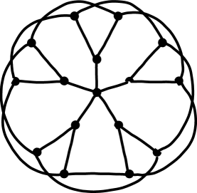
Figure 9: The generalized Petersen graph $P_{5,2}$.

Interest regarding these graphs comes from two sources. In [20] the problem is raised of finding the minimum number $e(n)$ of edges in a Class 0 graph on $n$ vertices. Because of the Petersen and Wheel graphs, we have $e(n)\leq 2n-2$. Blasiak, et al. [4], show that $e(n)\geq\lfloor 3n/2\rfloor$, and conjecture that $e(n)=3n/2+o(1)$. Furthermore, they believe that the graphs $P_{m,d}$ are all Class 0 which, if true, would prove the conjecture because it is $3$-regular except for the central vertex $u$, having degree $m$ (with $n=m(2^{d}-1)+1$). The graphs also appear in [12] as $n$-vertex graphs having the fewest edges among those of minimum degree 3 and radius $d$. In fact, the intuition for the conjecture comes from this result.

Here, we are most interested in the graphs $P_{m,2}$ for $m>3$. Note that $P_{m,2}$ has rotational symmetry: the exceptional edges for $k=2$ can be “rotated onward” by swapping $v_{1,0}$ with $v_{1,1}$ in the drawing. This makes $P_{m,2}$ transitive on the set $\{v_{i,X}\}$ for fixed length $X$. Thus, when calculating $\pi(P_{m,2})$, one only need consider the three vertices $u$, $v=v_{1,{\emptyset}}$, and $w=v_{1,0}$ as root.

      

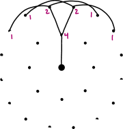
Figure 10: The graph $P_{8,2}$ and its main strategy $T$ for root $u$.

Theorem 14

For all $m\geq 4$ we have the following, where $n=n(P_{m,2})=3m+1$:

1. $\pi(P_{m,2},u)=n$,

2. $\pi(P_{m,2},v)\leq n+5$, and

3. $\pi(P_{m,2},w)\leq n+17$.

Proof.  When the root is $u$, we use all rotations of the following basic strategy $T$ (see Figure 10). Let $v_{1,{\emptyset}}$ have weight $4$, $v_{1,0}$ and $v_{1,1}$ have weight $2$, and each of their two neighbors have weight $1$. Clearly, of the sum of all rotations of $T$ has weight $4$ everywhere but $u$, and so the Uniform Covering Lemma applies.

When the root is $v$, we build slightly more complex strategies. First we use the nonbasic strategy $S$, having weight $3$ on $v_{0,0}$ and $v_{0,1}$ and weight $1$ on each of their neighbors. Next, write the rotations of $T$ as $T_{0},\ldots,T_{m-1}$. For $j\in\{0,1,2\}$, we build the basic strategies $S_{j}$ from these by combining all $T_{i}$ ($i\not=0$) with $i\equiv j\mod 3$, with the exception that if $j=1$ and $i=m-1$ then we do not include the vertices $v_{0,0}$ and $v_{0,1}$ twice. Moreover, each $S_{j}$ includes weight $8$ on $u$ (see Figure 11).

           

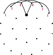
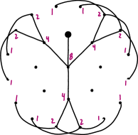
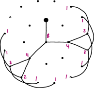
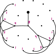
Figure 11: The four strategies for root $v$ in $P_{8,2}$.

One quarter of the sum of these four strategies has weight $0$ on $v$, weight $6$ on $u$, and weight $1$ everywhere else. Now the Weight Function Lemma (actually Corollary 3) applies.

The description for the strategies when the root is $w$ is almost identical to that for root $v$ (see Figure 12).

           

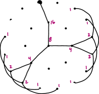
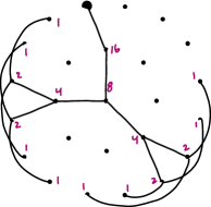
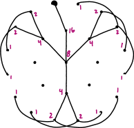
Figure 12: The four strategies for root $w$ in $P_{8,2}$.

In this case, one quarter of the sum of the four strategies has weight $0$ on $w$, weight $13.5$ on $v$, weight $6$ on $u$, and weight $1$ elsewhere. $\Box$

Next we define the generalized Coxeter $p$-graph $C(p)$ for odd primes $p=2q+1$. Like the graphs $P_{m,d}$, $C(p)$ has the potential (for $p\geq 5$) to be a Class 0 graph with fewer than $2n-2$ edges. Set $V_{i}=\{(i,j)\mid 0\leq j<p\}$ and $V=\cup_{i=0}^{q}V_{i}$, so that $C(p)$ has $n=p(q+1)=\binom{p+1}{2}$ vertices. Define the $2pq=2n-2p$ edges $(i,j)(i,j+1)$ and $(0,j)(i,j)$ for each $1\leq i\leq q$ and $0\leq j<p$. The vertices in $V_{0}$ have degree $q$ and all others have degree 3, making $C(7)$, the original Coxeter graph, 3-regular. Here we show the following $n+O(\sqrt{n})$ bound.

Theorem 15

For every prime $p\geq 11$ we have $\pi(C(p))\leq n+14q+14$.

Proof.  First we exhibit the symmetry of $G=C(p)$. To do so, we note that the arithmetic that follows will be modular in $q$ in the first coordinate, with the speciality that we use the representative $q$ in place of $0$, and modular in $p$ (as normal) in the second. Let ${\rho}$ be the automorphism that sends vertices $(i,j)$ to $(i,j+1)$ for all $0\leq i\leq q$ and $0\leq j<p$. This is a rotation of the vertices within each $V_{i}$. Let ${\alpha}$ generate $Z_{p}^{*}$ and define ${\sigma}$ to be the automorphism that sends $(0,j)$ to $(0,{\alpha}j)$ and $(i,j)$ to $(i+1,{\alpha}j)$ for all $1\leq i\leq q$ and $0\leq j<p$. While permuting $V_{0}$, the key aspect of ${\sigma}$ is that it also permutes the sets of vertices from $V_{i}$ to $V_{i+1}$. Together, ${\rho}$ and ${\sigma}$ act transitively on $V_{0}$ and on $\overline{V_{0}}$. This means that we only need calculate $\pi(G,(0,0))$ and $\pi(G,(1,0))$. (It turns out that $C(7)$ is fully vertex transitive and so the root $(0,0)$ suffices.)

Next we define the $q$ basic strategies ${\mathbf{T}}_{i}$ ($1\leq i\leq q$) for the root $r=(0,0)$, with each root child having weight 4. The child of $r$ in ${\mathbf{T}}_{i}$ has weight 4 and two children, $(i,i)$ and $(i,-i)$. We describe the descendents of $(i,i)$ only, as those of $(i,-i)$ are identical but with their second coordinate negated. The left subtree under $(i,i)$ is the path $(i,2i)$, $(i,3i)$, $\ldots$, $(i,qi)$. The right subtree under $(i,i)$ is a collection of $q-2$ paths, starting with children $(k,i)$ for $1\leq k\leq q$ with $k\not\in\{i,(p\pm i)/2\}$. The child $(k,i)=(k,sk)$, for $s=ik^{-1}$, and from it hangs the path $(k,(s+1)k)$, $\ldots$, $(k,qk)$.

Now we look at the sum of the weights of vertices over all strategies, and by the symmetries described above we need only consider the vertices $(i,j)$ for $i\in\{0,1\}$ and $0\leq j\leq q$. We note first that $(0,j)$ is the grandchild of $(j,0)$ in ${\mathbf{T}}_{j}$, and so has weight 1. The left path under $(1,1)$ shows that vertex $(1,j)$ has weight $2^{2-j}$ in ${\mathbf{T}}_{i}$. For $j\geq 3$ we see that if $k\leq j$ then vertex $(1,j)$ has weight $2^{k-j-1}$. Therefore, except for the $q$ weight 4 children of $r$ and their $2q$ weight 2 children, every other nonroot vertex has weight 1. This gives total weight $(n-1)+(4-1)q+(2-1)2q$, implying that $\pi(G,r)\leq n+5q$.

Consider the other root $r=(1,0)$. Here we need many more basic strategies — we will define ${\mathbf{T}}_{i}$ for $i\in\{\pm 1\}\cup\{2,\ldots,q\}$ — and the weights of the children of $r$ equal to 8 instead of 4. Similar to above, the strategy ${\mathbf{T}}_{-1}$ will be identical to ${\mathbf{T}}_{i}$ except that the second coordinates will be negated. We will describe the first four levels of each strategy explicitly, and their remaining levels implicitly. The child of $r$ in ${\mathbf{T}}_{1}$ is $(1,1)$, having children $(1,2)$ and $(0,1)$. From $(1,2)$ hangs the path $(1,3)$ and $(1,4)$, while the children of $(0,1)$ are $(2,1),\ldots(q,1)$. The children of each $(i,1)$ are $(i,1\pm i)$, subject to them not having already listed in some ${\mathbf{T}}_{j}$, which we now describe. The child of $r$ in ${\mathbf{T}}_{i}$ is $(0,0)$, which has the single child $(i,0)$. The two children of $(i,0)$ are $(i,\pm i)$, the two children of which are $(i,\pm 2i)$ and $(0,\pm i)$, correspondingly, with the exception that $(i,\pm 2i)$ does not appear in ${\mathbf{T}}_{q}$ because it already appears in ${\mathbf{T}}_{\pm 1}$ (as $(q,\pm 1)$). At this point, there are $q+1$ vertices of weight 8, $q+3$ vertices of weight 4, and $4q-2$ vertices of weight 2, with all other vertices having weight 1.

The remaining construction of the strategies proceeds in stages, with each new vertex added with several fractional weights adding up to 1. In the first stage, each vertex $(a,b)$ that is adjacent to a current leaf $(a,c)$ of some strategy is added to that strategy as a child of $(a,c)$, accounting for weight $1/2$. The other $1/2$ weight comes from adding it as a child of $(0,b)$ as well. In each subsequent stage, every vertex $(a,b)$ that is adjacent to a current leaf $(a,c)$ is added as a child of $(a,c)$ in every strategy that contains $(a,c)$, accounting for weight $1/2$. The other $1/2$ weight comes from adding it as a child of $(0,b)$ as well.

Hence we obtain $\pi(G,r)\leq(n-1)+7(q+1)+3(q+3)+1(4q-2)+1=n+14q+14$. $\Box$

We note that the number of strategies for the root $(1,0)$ can be reduced whenever two strategies (not including ${\mathbf{T}}_{\pm 1}$) share no vertices (other than $(0,0)$). Thus one can define the intersection graph $G_{p}$ of the family of sets $W_{i}$, $2\leq i\leq q$, where $W_{i}=V({\mathbf{T}}_{i})-\{(0,0)\}$. With chromatic number ${\chi}_{p}={\chi}(G_{p})$, we obtain the upper bound of $n+7{\chi}+7q+21$. For example, ${\chi}_{p}\leq 1$ when $p\leq 7$. In those cases, further improvements can be made as well, and it is not too hard to show that $\pi(C(5))\leq n+6$ and $\pi(C(7))\leq n+15$.

Finally, we discuss powers of cycles. For a given graph $G$ and integer $k$, we denote by $G^{(k)}$ the graph on the same vertex set as $G$, with edges $uv$ whenever the distance ${\sf dist}_{G}(u,v)\leq k$ in $G$. For example, $G^{(n-1)}=K_{n}$ for every connected $G$, where $n=n(G)$. Pachter, et al [20], define the pebbling exponent of $G$ to be the minimum $e=e_{\pi}(G)$ for which $G^{(e)}$ is Class 0. Consequently $e_{\pi}(G)\leq n-1$ for all $G$. The problem raised in [20] is to find $e_{\pi}(C_{n})$. Here we prove the following.

Theorem 16

The pebbling exponent of the cycle $C_{n}$ satisfies

$$\frac{n/2}{\lg n}\leq e_{\pi}(C_{n})\leq\frac{n/2}{\lg n-\lg\lg n}\ .$$

Proof.  The lower bound follows from the general fact that $\pi(G)\geq 2^{{\sf diam}(G)}$ for all $G$, along with the observation that ${\sf diam}(C_{n}^{(e)})=\lceil n/2e\rceil$. Therefore, a requirement for Class 0 is that $n\geq 2^{\lceil n/2e\rceil}$.

For the upper bound, we prove that $\pi(C_{n}^{(2^{k})})=n$ for $n=(2k+1)2^{k}+3=f(k)$. Then we show that $\pi(C_{n}^{(2^{k})})=n$ for $f(k-1)<n<f(k)$. Our method will be to split the cycle into two identical paths with endpoints at the root $r$, and use identical strategies on each one. We will invoke the Uniform Covering Lemma 6 to obtain the result.

In more detail, let us give a useful labeling of the vertices $V$ of $C_{n}$ as follows. We partition $V=\cup_{i=0}^{k+2}(U_{i}\cup W_{i})$ so that

• each $U_{i}$ and $W_{i}$ induces a path in $C_{n}$,

• $U_{0}=W_{0}=\{r\}$,

• $U_{i+1}$ follows $U_{i}$ when traversing $C_{n}$ clockwise from $r$,

• $W_{i+1}$ follows $W_{i}$ when traversing $C_{n}$ counterclockwise from $r$, and

• $U_{k+2}=W_{k+2}$.

The two identical paths mentioned above are seen to be $U=\cup_{i=0}^{k+2}U_{i}$ and $W=\cup_{i=0}^{k+2}W_{i}$, where now we see that the term ‘split’ was a white lie because of the overlap on $U_{k+2}=W_{k+2}$. We will describe a family ${\cal T}$ of strategies on $U$ with the property that, for some $m$ (actually $2^{k+1}$) and all $u\in\cup_{i=1}^{k+1}U_{i}$, we have $\sum_{T\in{\cal T}}T(u)=m$, while for all $u\in U_{k+2}$ we have $\sum_{T\in{\cal T}}T(u)=m/2$. Then we copy these strategies symmetrically onto $W$ and, because of the overlap, the Uniform Covering Lemma 6 applies.

Next we describe the vertices within each $U_{i}$. First, $|U_{i}|=2^{k}$ for $i\in\{1,k+2\}$, and $|U_{i}|=2^{k}-2^{k-i+1}$ for $2\leq i\leq k+1$ (thus $n=(2k+1)2^{k}+3$). We clockwise order the vertices of $U_{i}=\{v_{i,0},\ldots,v_{i,|U_{i}|-1}\}$ in their natural order by subscript, and will find it useful to identify $v_{i,j}$ with the encoding $[i,b_{j}]$, where $b_{j}$ is the $k$-bit binary representation of $j$ (so that leading zeros are not suppressed). For example, $v_{3,6}$ is encoded as $[3,00110]$ in $C_{355}$ since $k=5$ in that case. Also, the root $r$ is encoded as $[0,0^{k}]$, where we write $x^{j}$ to denote the concatenation $xx\cdots x$ of length $j$. Furthermore, we use the notation ${\mathbf{v}}_{j}$ to mean some binary word of length $j$, subject to context. That is, $[1,{\mathbf{v}}_{k}]$ is always a vertex in $U_{1}$ but $[2,{\mathbf{v}}_{k}]$ is not always in $U_{2}$ — every vertex in $U_{2}$ looks like $[2,0{\mathbf{v}}_{k-1}]$. Moreover, for $2\leq i\leq k+1$, vertices in $U_{i}$ look like everything but $[i,1^{i-1}{\mathbf{v}}_{k-i+1}]$.

Now we describe a partially ordered set $P$ that we will use to define our strategies. The elements of $P$ are the vertices $U$, and the covering relations are given by

1. $[0,0^{k}]>[1,{\mathbf{v}}_{k}]$ for all ${\mathbf{v}}_{k}$,

2. $[1,{\mathbf{v}}_{k-1}x]>[2,0{\mathbf{v}}_{k-1}]$ for all ${\mathbf{v}}_{k-1}$ and all $x\in\{0,1\}$,

3. $[i,{\mathbf{v}}_{i-1}{\mathbf{v}}_{k-i}x]>[i+1,{\mathbf{v}}_{i-1}b{\mathbf{v}}_{k-i}]$ for all $2\leq i\leq k$, all ${\mathbf{v}}_{i-1}\not=1^{i-1}$, all ${\mathbf{v}}_{k-i}$, and each $x,b\in\{0,1\}$,

4. $[i,1^{i-2}0{\mathbf{v}}_{k-i}x]>[i+1,1^{i-1}0{\mathbf{v}}_{k-i}]$ for all $2\leq i\leq k$, all ${\mathbf{v}}_{k-i}$, and all $x\in\{0,1\}$,

5. $[k+1,{\mathbf{v}}_{k}]>[k+2,{\mathbf{v}}_{k}]$ for all ${\mathbf{v}}_{k}\not=1^{k}$, and

6. $[k+1,1^{k-1}0]>[k+2,1^{d}]$.

All other relations of $P$ are determined by transitivity.

For $z\in P$, define its downset $D(z)=\{y\in P\mid y<z\}$. Notice that each $D=D([1,{\mathbf{v}}_{k}])$ forms a tree in $P$. Indeed, simple induction shows that if ${\mathbf{v}}_{k}=v_{1}\cdots v_{k}$ then every vertex of $U_{i+1}$ in $D$ has the form $[i+1,{\mathbf{x}}_{i}v_{1}\cdots v_{k-i}]$, where ${\mathbf{x}}_{i}$ is anything but $1^{i}$. This means that $[i+1,x_{1}\cdots x_{i}v_{1}\cdots v_{k-i}]$ has exactly one element from $D$ that covers it, namely either $[i,x_{1}\cdots x_{i-1}v_{1}\cdots v_{k-i}v_{k-i+1}]$ or $[i,x_{2}\cdots x_{i}v_{1}\cdots v_{k-i}v_{k-i+1}]$. So no cycles exist in $D$.

For each ${\mathbf{v}}_{k}$, then, define the basic strategy $T=T({\mathbf{v}}_{k})$ to have vertices $\{r\}\cup D([1,{\mathbf{v}}_{k}])$, with edge $zy$ whenever $z>y$ is a covering relation in $P$. In order that $T$ is a strategy in $C_{n}^{(2^{k})}$ we must verify that the distance $d={\sf dist}(z,y)$ between $z$ and $y$ in $C_{n}$ is at most $2^{k}$. When $z=r$, we have $y=v_{1,j}$ for some $0\leq j\leq 2^{k}-1$, so $d=j+1$. When $z=v_{1,j}$, we have $y=v_{2,\lfloor j/2\rfloor}$, so $d=2^{k}-\lceil j/2\rceil$. When $z=v_{i,j}$ and $2\leq i\leq k+1$, then we can write $j=h2^{k-i+1}+l$ for some $0\leq l<2^{k-i+1}$. From relation 3 or 4 we have $y=v_{2,j^{\prime}}$, where $j^{\prime}=h2^{k-i+1}+b2^{k-i}+\lfloor l/2\rfloor$ and $b\in\{0,1,2\}$. Thus the greatest distance comes from relation 4, in which case $d=|U_{i}|-j+j^{\prime}=2^{k}-\lceil l/2\rceil$.

Note that the characterization of elements in $D([1,{\mathbf{v}}_{k}])$ implies that each vertex of $U_{i}$ is in $2^{i-1}$ basic strategies when $1\leq i\leq k+1$, and in $2^{k}$ when $i=k+2$. Because each $T$ is basic, this means that $\sum_{T}T(v)=2^{k+1}$ for all $v\in U_{i}$ (resp. $W_{i}$), $1\leq i\leq k+1$, and $2^{k}$ for $v\in U_{k+2}$ (resp. $W_{k+2}$). Now the overlap from $U_{k+2}=W_{k+2}$ gives sum $m=2^{k+1}$ for all $v\not=r$, and the Uniform Covering Lemma 6 applies.

Finally, whenever $n$ is smaller than $f(k)$ we simply erase sufficiently many vertices of $U_{k+2}=W_{k+2}$ (but don’t renumber any indicies/encodings), as they are leaves in all strategies and so don’t destroy the uniform covering. When such vertices are exhausted continue erasing vertices of $U_{k+1}\cup W_{k+1}$ with similar results. Since $f(k)-f(k-1)=2^{k+1}$, no more considerations are necessary. $\Box$

4 Remarks

In this paper we have shown several different strengths of the Weight Function Lemma in combination with linear optimization, highlighting its versatility. It has been used to compute upper bounds on and exact values of the pebbling number of small graphs. It has also been successful in calculating the pebbling numbers of much larger graphs than previous algorithms. For such graphs having too many strategies than time allows to construct, the technique of creating a smaller set of them at random seems to perform just as well. This is most likely due to the property that nonoptimal solutions (derived from having fewer constraints) seem, in most instances, to be near optimal (have the same floor function). In fact, by restricting strategies to be breadth-first search, one obtains upper bounds on the greedy pebbling numbers of graphs (which requires pebbling steps to move toward the root). The method also yields results for many families of graphs, in many cases by hand, with much simpler and remarkably shorter proofs than given in previously existing arguments. This is especially so with highly symmetric graphs. We note also that the technique can be used in conjunction with more traditional arguments, as in Theorem 11, and it has delivered an array of upper bounds, such as $n$, $n+c$, and $n+o(n)$, most of which are the best known and might possibly be best possible. It’s two main shortcomings are the inability to overcome the kind of splitting structure found in cubes, for example, in which solutions to some configurations require nontree solutions, and the difficulty in dealing with large diameter, although success has been found with cycles and their graph powers, in addition to Petersen and Coxeter generalizations. When the technique gives upper bounds, it would be of great use to know how good the bound might be. That is, does the Weight Function Lemma yield an approximation algorithm for graph pebbling?

Question 17

Is there a constant $c$ such that, for all graphs $G$ and every root $r\in V(G)$, $z_{G,r}\leq c\pi(G,r)$?

For example, is $c=2$? The cube $Q^{d}$ shows that it couldn’t be any smaller.

Theorem 18

For all $d\geq 1$ and all $r\in V(Q^{d})$ we have $z_{Q^{d},r}<2\pi(Q^{d},r)$.

Proof.  We exploit the symmetry of $Q^{d}$ as follows. Because $Q^{d}$ is vertex transitive we need only consider one root $r$. We identify $V(Q^{d})$ with the power set of $\{1,\ldots,d\}$ and take $r={\emptyset}$. We define a single strategy ${\mathbf{T}}$ for $r$ and then apply every permutation of $\{1,\ldots,d\}$ to obtain other strategies. Finally we average over this collection of strategies. The result will be that $\pi(Q^{d})$ will be at most one more than the sum of the weights in this average.

For each $1\leq k\leq d$ such that $2^{k}\leq\binom{d}{k}$ we define $a_{k}=\lfloor\binom{d}{k}/2^{k}\rfloor$ and $b_{k}=\binom{d}{k}\mod 2^{k}$. We form ${\mathbf{T}}$ by first taking a neighbor of $r$. This neighbor will be a set of size 1, to which we assign the weight $2^{d-1}$ — this is step $i=1$, with $k=d-i$. For future steps $i$, while $2^{k}>\binom{d}{k}$, we continue adding a single neighbor, a set of size $i$, to the current leaf of ${\mathbf{T}}$, and assign the weight $2^{k}$. If $2^{k}\leq\binom{d}{k}$, however, we add $a_{k}+1$ vertices to the current leaves: $a_{k}$ of these will have weight $2^{k}$ and one will have weight $b_{k}$. All of these will be connected to leaves of weight $2^{k+1}$ and none will be connected to leaves of weight $b_{k+1}$. This is possible because the degree of each vertex of size $i-1$ is $k+1$, and $a_{k}<(k+1)a_{k+1}$ whenever $k+1<d-1$, so there are enough potential neighbors to accomplish this.

Hence we obtain weight $1$ on average for vertices of size $i$ for which $2^{k}\leq\binom{d}{k}$, and weight $2^{k}/\binom{d}{k}$ otherwise. This yields the bound $z_{Q^{d},r}\leq 1+\sum_{k=0}^{d-1}\max\{\binom{d}{k},2^{k}\}<\sum_{k=0}^{d}\binom{d}{k}+\sum_{k=0}^{d-1}2^{k}<2^{d+1}=2\pi(Q^{d})$. $\Box$

If one restricts their attention to only polynomially many strategies, this linear optimization technique becomes a polynomial algrorithm. It would be useful to investigate how good the approximation can be under these circumstances.

5 Acknowledgements

We thank Andrzej Czygrinow for converting the author’s Maple code for generating all the tree strategies of a rooted graph into java.

6 Appendix

6.1 Certificates for $R_{15}$

We list the missing certificates in order, with the all-zeros column signifying the root. The format is the same as that for $R_{15}$ at $v_{10}$ in Section 3.2. No attempt was made to find the simplest set of strategies.

$$\left(\begin{array}[]{r|rrrrrrrrrrrrrrr|r}577&0&8&4&0&0&0&2&4&0&2&0&0&2&1&2&25\\ 40&0&8&0&0&0&2&0&3&0&2&4&0&0&4&2&25\\ 1250&0&0&4&8&0&0&4&0&4&2&0&0&0&3&2&27\\ 542&0&0&0&0&8&0&2&4&0&2&4&1&2&2&2&27\\ 190&0&0&0&0&8&4&0&4&0&2&1&0&0&0&4&23\\ 217&0&0&0&0&8&4&1&4&0&2&4&0&2&0&4&29\\ 62&0&0&4&0&0&8&2&0&4&2&1&0&0&0&0&21\\ 646&0&0&0&0&0&8&0&2&4&2&1&0&4&4&0&25\\ 94&0&4&2&0&0&0&2&2&1&2&4&8&0&2&2&29\\ 91&0&8&4&0&0&1&0&4&2&2&4&2&2&4&2&35\\ 300&0&0&2&0&8&4&2&1&2&2&4&2&2&2&4&35\\ 344&0&4&0&0&0&2&2&2&0&2&4&8&4&1&2&31\\ 175&0&4&2&0&0&1&0&0&2&2&4&8&4&2&2&31\\ 472&0&4&2&0&0&1&2&2&2&2&4&8&4&0&2&33\\ \hline\cr&0&10004&10002&10000&9992&9998&9999&10000&10002&10000&9998&10004&10002&10001&9998&14000\\ \end{array}\right)$$

$$\left(\begin{array}[]{r|rrrrrrrrrrrrrrr|r}4&0&0&0&0&0&0&0&0&0&0&0&1&0&0&0&1\\ 4&0&0&0&0&0&0&0&0&0&0&0&0&0&1&0&1\\ 2&4&0&0&0&2&2&0&0&0&0&0&1&2&0&0&11\\ 2&0&0&4&0&0&2&1&0&0&0&0&0&0&0&0&7\\ 1&0&0&0&4&0&0&0&0&2&0&0&0&0&1&0&7\\ 1&0&0&0&4&0&0&2&0&2&0&0&0&0&1&0&9\\ 2&0&0&0&0&0&0&0&4&0&2&0&0&2&1&2&11\\ 2&0&0&0&0&2&0&2&0&2&2&4&1&0&0&2&15\\ \hline\cr&8&0&8&8&8&8&8&8&8&8&8&8&8&8&8&112\\ \end{array}\right)$$

$$\left(\begin{array}[]{r|rrrrrrrrrrrrrrr|r}2&0&8&0&0&2&0&0&4&0&2&1&4&2&0&0&23\\ 6&2&8&0&0&0&0&0&4&0&2&1&4&2&4&2&29\\ 34&2&8&0&0&0&0&0&4&0&2&4&4&2&3&2&31\\ 23&4&0&0&8&4&0&0&0&4&2&0&1&2&4&0&29\\ 1&0&0&0&0&0&8&0&0&4&2&1&2&4&0&0&21\\ 42&0&0&0&0&0&0&8&2&0&2&4&1&0&0&4&21\\ 16&4&0&0&8&4&0&0&2&4&2&1&2&2&4&0&33\\ 3&4&0&0&8&4&0&0&0&4&2&0&2&2&3&2&31\\ 19&0&0&0&0&4&8&0&2&4&2&0&1&4&0&2&27\\ 7&4&0&0&0&4&8&0&2&4&2&1&2&4&0&2&33\\ 15&4&0&0&0&4&8&0&0&4&2&0&2&4&3&2&33\\ \hline\cr&336&336&0&336&336&336&336&336&336&336&336&336&336&336&336&4704\\ \end{array}\right)$$

$$\left(\begin{array}[]{r|rrrrrrrrrrrrrrr|r}135&0&0&2&0&0&0&4&0&0&0&1&0&0&0&2&9\\ 31&0&0&0&0&0&4&0&0&8&4&3&0&2&0&0&21\\ 2&0&8&0&0&0&0&2&0&1&2&4&4&2&0&2&25\\ 1&2&4&8&0&0&4&0&0&1&0&2&2&2&0&0&25\\ 38&4&0&0&0&8&0&2&3&0&2&4&2&2&0&4&31\\ 10&2&0&0&0&0&4&0&0&8&4&4&2&0&1&2&27\\ 1&0&0&2&0&0&4&0&0&8&4&4&2&2&2&1&29\\ 103&0&4&2&0&1&0&0&4&0&2&0&2&2&8&2&27\\ 39&8&0&0&0&4&4&0&0&0&0&0&2&4&1&2&25\\ 30&8&2&1&0&0&4&0&2&0&0&0&4&4&0&0&25\\ 49&2&8&4&0&0&0&2&4&0&2&0&4&2&0&1&29\\ 4&2&8&4&0&0&1&2&0&0&2&4&4&0&4&0&31\\ 54&0&0&2&0&8&4&2&1&0&2&4&2&2&2&4&33\\ 82&2&1&2&0&0&4&2&2&8&4&4&2&2&0&0&33\\ \hline\cr&996&998&1000&0&995&996&998&1000&995&996&994&996&998&999&996&13957\\ \end{array}\right)$$

$$\left(\begin{array}[]{r|rrrrrrrrrrrrrrr|r}10&0&0&0&0&0&0&0&0&0&0&0&0&0&0&1&1\\ 6&4&0&0&0&0&0&0&0&0&0&0&2&1&0&0&7\\ 2&0&2&2&4&0&0&1&0&0&0&0&0&0&0&0&9\\ 1&0&0&2&4&0&0&2&0&0&0&0&0&0&1&0&9\\ 3&0&0&2&4&0&0&2&0&2&0&0&0&0&1&0&11\\ 6&0&0&2&0&0&4&0&0&1&0&0&0&2&2&0&11\\ 2&0&0&0&0&0&0&0&4&0&2&0&0&1&0&0&7\\ 2&0&2&0&0&0&0&0&4&0&2&0&0&0&2&1&11\\ 2&0&2&0&0&0&0&0&4&0&2&0&0&2&2&1&13\\ 6&0&2&0&0&0&0&2&0&2&2&4&2&0&0&1&15\\ 2&0&0&0&0&0&0&1&0&0&0&0&0&0&0&2&3\\ \hline\cr&24&24&24&24&0&24&24&24&24&24&24&24&24&24&24&336\\ \end{array}\right)$$

$$\left(\begin{array}[]{r|rrrrrrrrrrrrrrr|r}7&8&0&0&4&0&0&2&0&1&0&0&4&4&0&0&23\\ 5&8&0&0&0&4&0&0&0&0&0&0&4&3&0&2&21\\ 79&0&0&0&0&0&0&2&0&8&2&4&2&0&0&1&19\\ 1&0&4&2&3&0&0&0&0&0&0&0&2&0&8&0&19\\ 14&8&0&2&4&0&0&1&0&0&0&2&4&4&2&0&27\\ 120&2&4&8&3&0&0&4&0&0&0&0&2&0&0&2&25\\ 31&4&2&0&0&8&0&2&0&1&2&4&0&2&0&4&29\\ 91&0&0&0&4&8&0&2&1&0&2&4&2&0&0&4&27\\ 4&0&2&0&3&0&0&0&2&8&4&4&2&0&0&2&27\\ 20&4&0&0&0&0&0&0&4&0&2&0&1&8&0&0&19\\ 85&4&0&0&0&0&0&0&4&0&2&0&2&8&0&1&21\\ 104&0&4&0&0&0&0&0&4&0&2&0&1&0&8&0&19\\ 37&0&0&0&4&0&0&2&1&8&4&4&0&0&2&2&27\\ 7&2&4&1&4&0&0&2&4&0&2&0&2&0&8&2&31\\ \hline\cr&1006&998&997&999&996&0&998&1000&998&998&996&1002&1001&998&998&13985\\ \end{array}\right)$$

$$\left(\begin{array}[]{r|rrrrrrrrrrrrrrr|r}99&2&4&8&0&0&4&0&1&0&0&0&2&2&2&0&25\\ 26&2&4&8&0&0&4&0&2&2&0&0&2&2&1&0&27\\ 2&4&0&0&8&4&1&0&0&4&2&0&2&2&4&0&31\\ 59&0&0&0&0&0&0&0&1&2&2&4&2&1&0&0&12\\ 51&2&4&0&0&0&0&0&0&3&4&8&4&2&2&0&29\\ 31&0&0&0&0&4&0&0&1&4&4&8&4&2&0&0&27\\ 12&2&0&0&0&4&0&0&4&0&2&0&0&2&1&8&23\\ 65&0&0&0&0&4&2&0&4&0&2&0&0&2&1&8&23\\ 48&2&1&0&0&4&2&0&4&0&2&0&0&2&2&8&27\\ 123&4&2&0&8&3&2&0&2&4&2&0&2&2&4&0&35\\ 13&2&0&0&0&0&2&0&1&4&4&8&4&2&0&0&27\\ \hline\cr&998&998&1000&1000&1001&1000&0&1000&999&998&996&998&999&999&1000&13986\\ \end{array}\right)$$

$$\left(\begin{array}[]{r|rrrrrrrrrrrrrrr|r}203&0&0&0&0&0&0&0&0&2&4&1&0&0&0&0&7\\ 208&2&0&0&0&0&1&0&0&0&0&0&2&4&0&0&9\\ 7&0&0&2&4&8&0&0&0&2&0&3&0&0&0&0&19\\ 66&0&0&0&4&0&4&1&0&2&0&0&0&0&8&0&19\\ 37&2&3&2&4&0&4&2&0&0&0&0&0&0&8&0&25\\ 116&0&0&2&1&0&0&4&0&0&0&0&0&0&0&8&15\\ 38&4&8&4&0&0&2&2&0&2&1&4&2&2&4&0&35\\ 30&4&0&2&0&8&4&0&0&2&0&0&2&0&1&0&23\\ 5&2&0&2&4&8&4&2&0&0&0&0&0&1&0&0&23\\ 77&2&0&2&4&8&0&2&0&2&1&4&2&0&0&0&27\\ 6&0&0&2&0&8&4&2&0&2&0&4&0&0&0&1&23\\ 37&0&8&4&0&0&2&2&0&2&2&4&4&2&0&1&31\\ 6&2&8&4&0&0&1&2&0&2&0&4&4&2&0&0&29\\ 31&2&8&4&4&0&2&2&0&2&0&4&4&0&0&1&33\\ \hline\cr&1000&1007&1004&1008&1000&1002&1004&0&1002&1001&1004&1002&999&1006&1002&14041\\ \end{array}\right)$$

$$\left(\begin{array}[]{r|rrrrrrrrrrrrrrr|r}82&2&0&2&4&0&0&8&0&1&0&0&0&0&2&0&19\\ 15&0&0&2&4&0&0&8&0&2&0&0&0&0&2&3&21\\ 98&0&0&0&0&0&2&0&1&0&0&0&8&4&0&0&15\\ 3&0&0&0&0&0&0&0&4&0&2&0&0&0&1&8&15\\ 12&0&0&0&0&0&0&0&4&0&2&0&0&1&2&8&17\\ 4&0&8&4&4&0&1&0&0&2&0&0&4&0&4&0&27\\ 38&4&8&4&0&0&0&1&4&0&0&0&4&2&4&2&33\\ 11&0&8&4&4&0&2&0&4&2&0&0&3&0&4&0&31\\ 67&2&0&2&0&8&4&0&1&2&0&0&0&2&2&4&27\\ 58&4&0&2&0&8&4&1&0&2&0&0&0&0&2&4&27\\ 14&2&0&4&4&0&1&8&0&0&0&0&0&0&2&0&21\\ 120&0&0&0&2&0&1&0&4&4&8&0&0&2&0&2&23\\ 64&4&8&4&4&0&2&0&1&2&0&0&0&2&4&0&31\\ 8&4&8&4&0&0&2&2&4&0&1&0&2&2&4&2&35\\ \hline\cr&998&1000&1000&1000&1000&1000&1000&997&1000&998&0&1001&998&999&997&13988\\ \end{array}\right)$$

$$\left(\begin{array}[]{r|rrrrrrrrrrrrrrr|r}28&8&0&2&4&3&0&2&0&2&0&0&0&0&2&0&23\\ 4&8&0&0&4&2&3&2&0&2&0&0&0&0&2&0&23\\ 3&0&0&0&0&4&0&4&0&1&4&8&0&0&0&0&21\\ 4&0&0&2&0&3&0&4&0&0&4&8&0&0&0&0&21\\ 27&8&0&2&4&4&2&2&0&1&0&0&0&0&2&2&27\\ 33&0&8&4&4&1&2&2&4&0&2&0&0&0&4&2&33\\ 52&0&0&0&0&2&1&4&0&4&4&8&0&0&0&4&27\\ 59&0&0&2&0&1&4&0&4&2&2&0&0&8&2&2&27\\ 26&0&8&4&4&2&2&2&4&2&2&0&0&0&4&1&35\\ \hline\cr&472&472&472&472&472&472&472&472&472&472&472&0&472&472&472&6608\\ \end{array}\right)$$

$$\left(\begin{array}[]{r|rrrrrrrrrrrrrrr|r}8&8&0&2&4&0&0&2&0&1&0&0&0&0&2&0&19\\ 10&0&0&0&0&0&0&2&0&1&2&4&8&0&0&2&19\\ 15&8&0&2&4&4&0&2&0&0&0&0&0&0&2&1&23\\ 14&8&0&0&4&4&0&2&0&2&0&0&0&0&2&1&23\\ 5&0&2&4&0&3&8&2&0&4&2&2&0&0&4&0&31\\ 13&0&4&0&2&1&0&2&8&0&4&2&0&0&4&4&31\\ 27&0&4&2&1&0&0&2&0&2&2&4&8&0&2&2&29\\ 2&0&2&4&0&4&8&2&0&4&2&2&0&0&0&1&29\\ 17&0&0&4&2&4&8&2&0&4&2&2&0&0&0&1&29\\ 13&0&2&4&1&4&8&2&0&4&2&2&0&0&0&2&31\\ 24&0&4&2&2&1&0&2&8&2&4&2&0&0&4&4&35\\ \hline\cr&296&296&296&296&296&296&296&296&296&296&296&296&0&296&296&4144\\ \end{array}\right)$$

$$\left(\begin{array}[]{r|rrrrrrrrrrrrrrr|r}19&2&4&2&0&4&0&0&8&0&4&2&2&0&0&3&31\\ 109&0&8&4&0&0&0&2&0&0&1&4&4&2&0&2&27\\ 3&0&0&2&8&3&0&4&0&4&2&2&0&0&0&0&25\\ 22&0&0&0&0&4&1&2&8&0&0&2&2&4&0&4&27\\ 27&2&0&0&0&1&0&0&8&0&4&0&0&4&0&4&23\\ 30&0&0&0&0&2&1&0&8&0&4&0&2&4&0&4&25\\ 16&0&0&0&0&0&0&2&8&2&4&0&0&3&0&4&23\\ 3&2&8&4&0&2&1&2&4&0&2&0&4&0&0&0&29\\ 7&4&0&4&8&4&0&1&2&4&2&2&0&0&0&2&33\\ 116&4&0&0&8&4&0&4&0&4&2&2&2&1&0&2&33\\ 54&4&0&4&0&2&8&2&0&4&2&2&2&1&0&0&31\\ 28&2&0&4&0&0&8&1&0&4&2&2&2&4&0&0&29\\ 35&4&0&4&0&4&8&2&0&4&2&2&0&3&0&2&35\\ 8&0&4&2&0&0&1&2&8&0&4&0&2&4&0&4&31\\ \hline\cr&1002&1004&1004&1008&1006&999&1005&1002&1004&1001&1004&1002&1001&0&1003&14045\\ \end{array}\right)$$

$$\left(\begin{array}[]{r|rrrrrrrrrrrrrrr|r}14&4&2&2&4&8&2&0&0&1&0&0&2&2&0&0&27\\ 6&4&2&2&1&8&4&0&0&2&0&0&2&2&0&0&27\\ 1&4&2&0&2&8&4&0&0&1&0&0&2&2&2&0&27\\ 5&4&0&2&2&8&4&0&0&1&0&0&2&2&2&0&27\\ 2&2&1&4&4&0&2&8&0&0&0&0&0&0&0&0&21\\ 14&2&2&4&4&0&1&8&0&0&0&0&0&0&2&0&23\\ 10&2&0&4&4&0&1&8&0&2&0&0&0&0&2&0&23\\ 2&2&4&1&2&0&2&0&8&2&4&0&2&4&0&0&31\\ 24&2&1&0&0&0&2&0&8&2&4&0&2&4&4&0&29\\ 26&0&4&2&1&0&2&0&0&4&4&8&4&2&2&0&33\\ \hline\cr&208&208&208&208&208&208&208&208&208&208&208&208&208&208&0&2912\\ \end{array}\right)$$

6.2 Certificates for $R_{20}$

We list the missing certificates in order, as above.

References

- [1] A. Bekmetjev and A. Cusack, Pebbling algorithms in diameter two graphs, SIAM J. Disc. Math. 23, no. 2, (2009), 634–646.
- [2] A. Bekmetjev, G. Brightwell, A. Czygrinow and G. Hurlbert, Thresholds for families of multisets, with an application to graph pebbling, Discrete Math. 269 (2003), no. 1-3, 21–34.
- [3] A. Bekmetjev and G. Hurlbert, The pebbling threshold of the square of cliques, Discrete Math., 308 no. 19 (2008), 4306–4314.
- [4] A. Blasiak, A. Czygrinow, A. Fu, D. Herscovici, G. Hurlbert and J. Schmitt, Sparse graphs with small pebbling number, preprint.
- [5] A. Blasiak and J. Schmitt, Degree sum conditions in graph pebbling, Australas. J. Combin. 42 (2008), 83–90.
- [6] P. Chiu, Cubic Ramanujan graphs, Combinatorica 12 (1992), no. 3, 275–285.
- [7] F. R. K. Chung, Pebbling in hypercubes, SIAM J. Disc. Math. 2 (1989), no. 4, 467–472.
- [8] T. Clarke, R. Hochberg and G. Hurlbert, Pebbling in diameter two graphs and products of paths, J. Graph Th. 25 (1997), no. 2, 119–128.
- [9] A. Czygrinow and G. Hurlbert, Girth, pebbling, and grid thresholds, SIAM J. Discrete Math., 20 no. 1 (2006), 1–10.
- [10] A. Czygrinow and G. Hurlbert, On the pebbling threshold of paths and the pebbling threshold spectrum, Discrete Math., 308 no. 15 (2008), 3297–3307.
- [11] A. Czygrinow, G. Hurlbert, H. Kierstead, and W.T. Trotter, A note on graph pebbling, Graphs and Combinatorics 18 (2002), 219–225.
- [12] P. Dankelmann and L. Volkmann, Minimum size of a graph or digraph of given radius, Inform. Process. Lett. 109 (2009), no. 16, 971–973.
- [13] D. Herscovici, Graham’s pebbling conjecture on products of many cycles, Discrete Math. 308 (2008), no. 24, 6501–6512.
- [14] G. Hurlbert, A survey of graph pebbling, Congr. Numer. 139 (1999), 41–64.
- [15] G. Hurlbert, Recent progress in graph pebbling, Graph Theory Notes of New York XLIX (2005), 25–37.
- [16] G. Hurlbert, General graph pebbling, Discrete Appl. Math., to appear (2010).
-
[17]
G. Hurlbert,
The Graph Pebbling Page,
http://mingus.la.asu.edu/~hurlbert/pebbling/pebb.html. - [18] G. Hurlbert and H. Kierstead, Graph pebbling complexity and fractional pebbling, unpublished (2005).
- [19] K. Milans and B. Clark, The complexity of graph pebbling, SIAM J. Discrete Math. 20 (2006), no. 3, 769–798.
- [20] L. Pachter, H. Snevily and B. Voxman, On pebbling graphs, Congr. Numer. 107 (1995), 65–80.
- [21] N. Sieben, A graph pebbling algorithm on weighted graphs, J. Graph Algorithms Appl. 14 (2010), no. 2, 221–244.
- [22] N. Watson, The complexity of pebbling and cover pebbling, arXiv:math/0503511 (2005).