Initial data transients in binary black hole evolutions
Abstract
We describe a method for initializing characteristic evolutions of the Einstein equations using a linearized solution corresponding to purely outgoing radiation. This allows for a more consistent application of the characteristic (null cone) techniques for invariantly determining the gravitational radiation content of numerical simulations. In addition, we are able to identify the ingoing radiation contained in the characteristic initial data, as well as in the initial data of the 3+1 simulation. We find that each component leads to a small but long lasting (several hundred mass scales) transient in the measured outgoing gravitational waves.
pacs:
04.25.dg, 04.30.Db, 04.30.Tv, 04.30.Nk1 Introduction
It is well known in numerical relativity that current practice for the setting of initial data introduces spurious radiation into the system, in both the 3+1 and the characteristic approaches. The error in the initial data leads to an initial burst of spurious “junk” radiation that results from solving the constraint equations on a single hypersurface, without knowing the past history of the radiation content. Common practice regards the signal as physical only after it has settled down following the burst arising from the initial data solution. While it is straightforward to handle the junk radiation in this way, a more serious issue is whether the spurious radiation content of the initial data leads to longer-term transients in the wave signal. This question has been considered before, but previous work on the long-term effect of the initial data is limited [1, 2, 3, 4].
Characteristic extraction is a method of invariantly measuring the gravitational wave emission of an isolated source by transporting the data to null infinity () using a null formulation of the Einstein equations [5, 6, 7, 8, 9, 10]. Initial data is needed on a null cone in the far field region, say . Previous work has taken the simplistic approach of setting the null shear everywhere, although a recent investigation sets by the condition that the Newman-Penrose quantity [10]. Setting shear-free initial data is not necessarily incorrect physically – for example in the Schwarschild geometry in natural coordinates everywhere, and it is possible to construct a radiating solution with everywhere at a specific time. However in the generic case, a radiating solution has , and imposing in effect means that the outgoing radiation implied by the boundary data must be matched at the initial time by ingoing radiation. In principle, the spurious incoming content of data extends out towards infinity, and so could contaminate the entire evolution. However, previous results comparing characteristic extraction with conventional finite radius extrapolation indicate that it is at most a minor effect [8, 9].
Since the characteristic initial data is needed only in the far field region, linearized theory provides a suitable approximation. That is, it is possible to construct initial data that, at the linearized approximation, represents the physical situation of a gravitational field with purely outgoing radiation produced by sources in a central region [11]. We first solve the case of two equal mass objects in circular orbit around each other in a Minkowski background as a model analytic problem.
We then develop and implement a procedure to calculate characteristic metric data that contains purely outgoing radiation. This is done within the context of characteristic extraction, so that initial data on the null cone is constructed that is compatible with given data on a worldtube at constant radius. We are then able to compare the waveforms computed by characteristic extraction using as initial data (a) , and (b) the linearized solution. We find that while the dominant gravitational wave modes are largely unaffected by the choice of initial , a small residual difference is visible between the two approaches, and can take several hundred to be damped below other effects.
Any mis-match between the linearized solution and the actual data is an indication of an ingoing radiation content. Now, on the worldtube , the characteristic metric data is determined entirely by the 3+1 data so that any ingoing radiation can be traced back to an ingoing radiation content in the conformally flat 3+1 initial data. In this way we show that the 3+1 initial data contains a component of ingoing radiation which results in a long-lasting transient.
The plan of the paper is as follows. Sec. 2 introduces the notation, and reviews results needed from previous work. Sec. 3 applies linearized characteristic theory to calculate metric data for two equal mass non-spinning black holes in circular orbit around each other. Sec. 4 describes the method to construct metric data everywhere from data on a worldtube. Sec. 5 describes our numerical results, which are obtained within the context of a binary black hole inspiral and merger. The paper ends with Sec. 6, Discussion and Conclusion.
2 Review of results needed from other work
2.1 The Bondi-Sachs metric
The formalism for the numerical evolution of Einstein’s equations, in null cone coordinates, is well known [12, 13, 14, 15, 16, 17]. For the sake of completeness, we give a summary of those aspects of the formalism that will be used here. We start with coordinates based upon a family of outgoing null hypersurfaces. Let label these hypersurfaces, label the null rays, and be a surface area coordinate. In the resulting coordinates, the metric takes the Bondi-Sachs form [12, 18]
| (1) | |||||
where and , with a metric representing a unit 2-sphere; is a normalized variable used in the code, related to the usual Bondi-Sachs variable by . As discussed in more detail below, we represent by means of a complex dyad . Then, for an arbitrary Bondi-Sachs metric, can be represented by its dyad component
| (2) |
with the spherically symmetric case characterized by . We also introduce the fields
| (3) |
as well as the (complex differential) eth operators and [19].
In the Bondi-Sachs framework, Einstein’s equations are classified as: hypersurface equations – – forming a hierarchical set for and ; evolution equation for ; and constraints . An evolution problem is normally formulated in the region of spacetime between a timelike or null worldtube and future null infinity (), with (free) initial data given on , and with boundary data for satisfying the constraints given on the inner worldtube. We extend the computational grid to by compactifying the radial coordinate by means of a transformation
| (4) |
In characteristic coordinates, the Einstein equations remain regular at under such a transformation.
The free initial data for essentially determines the ingoing radiation content at the beginning of the evolution. For the case of binary black hole evolutions in a 3+1 formalism, the initial Cauchy data is determined by solving the Hamiltonian and momentum constraints, usually under the assumption of conformal flatness. Compatible null data initial solutions are not known, and so we must choose an ansatz for which is approximately compatible. Previous work [8, 9] has simply set . In Section 3, we propose a refinement whereby is set according to a linearized solution which is determined by the Cauchy initial data solution.
2.2 The spin-weighted formalism and the operator
A complex dyad is a 2-vector whose real and imaginary parts are unit vectors that are orthogonal to each other. Further, represents the metric, and has the properties
| (5) |
Note that is not unique, up to a unitary factor: if represents a given 2-metric, then so does . Thus, considerations of simplicity are used in deciding the precise form of dyad to represent a particular 2-metric.
Having defined a dyad, we may construct complex quantities representing angular tensor components on the sphere, for example , , . Each object has no free (angular) indices, and has associated with it a spin-weight defined as the number of factors less the number of factors in its definition. For example, , and, in general, . We define derivative operators and acting on a quantity with spin-weight
| (6) |
where the spin-weights of and are and , respectively, and where
| (7) |
Some commonly used dyad quantities are
| (8) |
The spin-weights of the quantities used in the Bondi-Sachs metric are
| (9) |
We will be using spin-weighted spherical harmonics [20, 21] , where the suffix s denotes the spin-weight, and in the case the will be omitted i.e. . It is convenient to make use of the formalism described in [22, 11], and have basis functions whose spin-weight 0 components are purely real; following [11], these are denoted as . Note that the effect of the operator acting on is
| (10a) | |||||
| (10b) | |||||
2.3 Solutions to the linearized Einstein equations
Ref. [11] (see also [23]) obtained solutions to the linearized Einstein equations in Bondi-Sachs form using the ansatz
| (10k) |
for a metric coefficient with spin-weight . Here, we need the results for linearization about a Minkowski background, in which the spacetime is vacuum everywhere except on a spherical shell at . Strictly speaking, we should be performing the linearization about a Schwarzschild (or even Kerr) background rather than about Minkowski. In the Kerr case it is not known how to do so, and in the Schwarzschild case the difference is that, in Eq. (10lb), the term is replaced by a term whose leading-order behaviour is also but which is not representable analytically. We consider the lowest order case and in the exterior of the shell (i.e., ), and describe that part of the solution that represents purely outgoing gavitational radiation.
| (10la) | |||||
| (10lb) | |||||
| (10lc) | |||||
| (10ld) | |||||
The solution is determined by setting the constant (real valued) parameters , and . The gravitational news corresponding to this solution is given by
| (10lm) |
We will also need the solution in the case in the exterior region
| (10lna) | |||
| (10lnb) | |||
| (10lnc) | |||
| (10lnd) |
in terms of the additional parameters , and .
3 Black hole binaries in circular orbit: Solution in the linearized limit
The linearized solution described in the previous section will be used to set initial data on the null cone. We seek a solution which corresponds roughly to the source of the gravitational radiation which we will eventually measure, namely a binary black hole system. In order to be able to apply the linearized theory, we model each black hole as having a matter density that is described by a Dirac- function whose location moves uniformly around a spherical shell. More precisely, the matter density in the spacetime is
| (10lno) |
with respect to Bondi-Sachs coordinates . The mass of each black hole is , the circular orbit has radius , and the black holes move with angular velocity . We next express in terms of spherical harmonics
| (10lnp) |
and apply the usual procedure, that is multiplication by followed by integration over the sphere, to determine the coefficients . We find that, for , the only nonzero coefficients are
| (10lnq) |
In linearized form, the Einstein equation is
| (10lnr) |
where is the covariant component of velocity in the -direction. Imposing the gauge condition that the coordinates should be such that, on the worldline of the origin, the metric takes Minkowski form, it follows that there and consequently at all points within . Expanding in terms of spherical harmonics
| (10lns) |
and integrating Eq. (10lnr), we find the coefficients for ,
| (10lnt) |
The determination of the remaining metric coefficients depends on the value of . The case is straightforward, and we find for
| (10lnu) |
The case uses the results for a static shell on a Minkowski background in [11]. We solve the jump conditions across the shell for the various metric quantities 111Maple script for this purpose (nu0_regular_0.map with output in nu0_regular_0.out) are provided in the supplementary data.. The result is, in the interior,
| (10lnv) |
and in the exterior
| (10lnwa) | |||||
| (10lnwb) | |||||
The cases use the results for a dynamic shell on a Minkowski background in [11] 222The calculation is provided in the Maple script regular_0.map with the output in regular_0.out in the supplementary data.. The script constructs the general solution inside and outside the shell , and uses the constraint equations, as well as regularity conditions at the origin and at infinity, to eliminate some of the unknown coefficients. It imposes the jump conditions at the shell, and finds a unique solution for the remaining unknowns. The result in the exterior is
| (10lnwxa) | |||||
| (10lnwxb) | |||||
where
| (10lnwxy) |
and takes the form given in Eq. (10lb). The gravitational news is
| (10lnwxz) | |||||
Although the coefficient is complicated, it can be expressed to leading order in
| (10lnwxaa) |
It follows that, again to leading order in , the news is
| (10lnwxab) | |||||
from which it is easy to deduce, via the Bondi relation, that the rate of energy loss of the system is
| (10lnwxac) |
In the limit of a low velocity circular orbit, , , the above formula reduces to
| (10lnwxad) |
which is identical to that found from the standard quadrupole formula [24].
4 Constructing the metric from data on a worldtube
In characteristic extraction, the Cauchy evolution provides the characteristic metric variables and on the worldtube , decomposed into spherical harmonics , at every time step. In this section, we develop a method to find coefficients of the linearized solutions that provide a fit to the actual numerical data at the worldtube (to linear order and excluding incoming radiation). Then we use the linearized solutions with the coefficients just found to predict everywhere at some chosen time , and in this way provide initial data for a numerical characteristic evolution. We restrict attention to the dominant modes . The method uses a Fourier decomposition in the time domain, and works well when the data is approximately sinusoidal, with amplitude and frequency varying slowly. Accordingly, for the binary black hole computation, the method is applied over a time domain that excludes both the junk radiation and the merger.
A metric variable may be written as
| (10lnwxae) |
where ∗ denotes the complex conjugate. The relationship between the coefficients of and follows theoretically from the requirement that the spin weight 0 metric components must be real; and further the metric data has been checked to confirm that it does satisfy the relationship. Transforming to the basis, we find
| (10lnwxaf) |
where
| (10lnwxag) |
so that the metric data on can be re-expressed as coefficients of , and at discrete time values. Although the data is oscillatory in time, it is not at constant frequency but is a superposition of multiple solutions with different frequencies. The linearized solutions behave as for fixed , so for the theory to be applicable the next step is to decompose the metric data into a superposition of constant frequency components. This is achieved by making a discrete fast Fourier transform of each metric coefficient
| (10lnwxah) |
where there are data points over the time interval . The frequency is related to by
| (10lnwxai) |
We found that at from the linearized solutions provides a smoother fit to the actual data if high frequencies are eliminated (compare Sec. 5, Fig. 1), and so we undertake further processing only for (with ); the setting of the Fourier coefficients for is described later.
In the case , for each value of Eqs. (10la) to (10ld) evaluated at the worldtube are four equations for the three unknowns . Such an over-determined system can be tackled by a least-squares-fit algorithm, or alternatively by ignoring one of the equations so making the system uniquely determined. We found that the reconstructed linearized solution gave a better fit to the actual data at in the case that Eq. (10ld) for was ignored. This then means that a comparison between the actual and reconstructed data for at the worldtube provides an indication of the error, which is expected because of (a) incoming radiation in the initial Cauchy data, (b) Fourier transform effects, and (c) other effects. We discuss item (b) at the end of this section, and items (a) and (c) in the next section.
In the case , , and Eqs. (10lna) to (10lnd) are four equations for the constants . We solved four equations for three unknowns using a least-squares-fit algorithm, because this approach led to the reconstructed data having a better fit to the actual data than in the case that Eq. (10lnd) was ignored.
In this way, for a given spherical harmonic say , we obtain values for the constants of the frequencies represented by . Now, our purpose is to use the worldtube data to estimate off the worldtube. From Eq. (10lb) we can write
| (10lnwxaj) |
where for
| (10lnwxaka) | |||||
| (10lnwxakb) | |||||
| (10lnwxakc) | |||||
and for
| (10lnwxakal) |
We then apply the inverse discrete Fourier transform to find
| (10lnwxakam) |
where for , and
| (10lnwxakan) |
Eq. (10lnwxakan) follows from the condition that (and all other coefficients in the time domain) are real. The functions and are found in a similar way, and so we are able to find the coefficient of of a given spherical harmonic, say . Repeating the calculation for the other spherical harmonics and leads to a prediction of to lowest order .
The coefficient of is not oscillatory, but can rather be described as slowly varying. While in principle, such behaviour can be represented by a Fourier decomposition, we found that a better fit was obtained by regarding the solution as almost constant and solving Eqs. (10lna) to (10lnc) at each time step, with Eq. (10lnd) used as a measure of the error 333The Matlab scripts ft_wt_driver.m, FT_WT.m and nu0.m are provided in the supplementary data..
We investigated the possibility of errors introduced in the Fourier transform and inverse transform process by comparing on the worldtube the actual and reconstructed values of , and , because the construction is such that they should be identical444Note that is not necessarily identical, since there are may be differences due to nonlinearities and incoming radiation.. The following comparison is for the R100 case as specified in the next section. We found that there was essentially no difference between the original and reconstructed data, apart from minor variations over about the first and last of the time interval (of total duration ), presumably caused by the cut-off of high frequencies. This test was performed for both and with no visible difference seen in the graphs, indicating that the precise way in which high frequencies are removed is not important.
5 Numerical results
| Worldtube location | Initial time | Initial data | |
|---|---|---|---|
| Data set | |||
| J0-R100-u0 | |||
| J0-R250-u0 | |||
| J0-R100-u450 | |||
| J0-R250-u900 | |||
| Jlin-R100-u450 | |||
| Jlin-R250-u900 |
We apply the method outlined in the previous section to the problem of measuring gravitational waves from binary black hole simulations. Following our implementation of characteristic extraction [8, 9], we first evolve a spacetime with a 3+1 (Cauchy) evolution code, recording metric data on a world tube, , of fixed coordinate radius. This data is subsequently used as inner boundary data for a null-cone evolution of the Einstein equations, which transports the data to , where the gravitational waves are measured. The linearized solution allows us to specify data for on the initial null cone which is compatible (to the linear level) with the data on and thus, importantly, to the Cauchy 3+1 spacetime.
As a fiducial test case, we return to the well-studied model of an 8-orbit binary system with equal mass non-spinning black holes carried out in [8, 9]. For the Cauchy evolution, we use the Llama multipatch code described in [25, 26]. We output metric data on two worldtubes located at and that are used as inner boundary data for a subsequent characteristic evolution. The waveforms at should be independent of the worldtube location. Thus, evolutions from different worldtube locations help us validate our results. Table 1, summarizes the various characteristic evolutions that we have performed, all of which are based on the same Cauchy data, but with different characteristic initial data, , and starting points in Bondi time, .
The first approach follows the original prescription laid out in [8, 9]. The characteristic evolution is started coincident with the first available Cauchy data, at coordinate time . The characteristic variable is initialized by the shear-free solution . Since we are beginning the characteristic evolution from the initial Cauchy slice, these models include the spurious junk radiation contained in the conformally flat constraint solution. Models J0-R100-u0 and J0-R250-u0 listed in Table 1 follow this prescription, using data from the worldtubes at and , respectively.
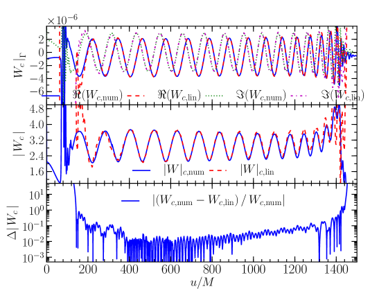
It is interesting to compare the results of the fully nonlinear characteristic Einstein evolution with the corresponding linearized solution. Fig. 1 plots the spherical harmonic modes of , computed by the null Einstein evolution J0-R100-u0. The linearized solution is computed using linearly reconstructed worldtube data according to the prescription in Sections 3 and 4. We compute the linearized solution from the boundary data at after the initial data junk radiation has passed the worldtube radius , at around , when the system has settled to the expected binary black hole inspiral pattern compatible with the solution construction. The upper panel of Fig. 1 plots the real and imaginary parts of , evaluated at . The center panel plots the amplitudes of , while the bottom panel shows the relative difference between the linearly estimated and the fully relativistic result (model J0-R100-u0). The linearized and numerically evolved differ initially, but eventually, after around , differ by less that , which remains consistent for the bulk of the time.
We first discuss whether the difference between the solutions can be due to effects other than ingoing radiation; such effects could include (a) nonlinearity, or (b) the linearization background being Minkowski rather than Schwarzschild. Looking at Figs. 1 and 2, we see that to lowest order the metric components are slowly varying sinusoidal functions; this statement also applies to the other metric components (graphs not shown). We would therefore expect that the magnitude of effects (a) and (b) would be roughly constant, if not with some increase at later times as merger is approached. Indeed for nonlinear effects we can look at the Einstein equation for , which is to linear order, with the actual value being an indication of the magnitude of nonlinearity, and we find that this quantity does slowly increase with time. However, Figs. 1 and 2 show that the difference between the solutions, until about , is getting smaller. This indicates that the effect is independent of non-linearities and present already at the linear level. The linearized solution assumes that the radiation is purely outgoing, whereas the actual data may contain incoming modes originating in either the characteristic or Cauchy initial data – both options being possible since at is influenced by both data sets. Thus, the explanation for Fig. 1 is that it reflects the slow decay of the effect of incoming modes in the initial data, until saturated by other factors (such as non-linear effects).

A similar effect is seen in the characteristic variable , related to the Newtonian potential, plotted in Fig. 2. In this case, however, there is clarity about the source of the incoming radiation: it must be in the Cauchy data. This is because in characteristic extraction, the characteristic metric at the worldtube is determined entirely by the Cauchy data. Again, the lower panel shows an approximately exponential decay in the differences, until around . The residual steady state differences result from other effects, which gradually increase with the strength of the gravitational radiation towards the binary merger.
The findings above indicate that a physically expected purely outgoing inspiral radiation pattern is only present after some time
| (10lnwxakao) |
where is the length of a time interval until the incoming radiation content of the Cauchy initial data has settled to a negligible amount at the given worldtube location. Hence, in order to construct physically meaningful and consistent initial data via the outgoing linearized solution, it is optimal to begin the solution at a time after which both the junk and incoming radiation content of the initial data have subsided. The results of Figs. 1 and 2 suggest that the linearized solution provides a reasonably good approximation to the data , at which time the system has settled into an outgoing radiative solution.
For instance, in model Jlin-R100-u450, the exact worldtube location is . Allowing for the visible outgoing junk radiation to pass, we set the time range over which we use the boundary data for linearized solution construction to , which includes the inspiral, but not the merger and ringdown. The time increment in is given by , thus comprising 8967 data points. Referring to Eq. (10lnwxah), we have , . In order to determine at the initial time , we use the general form of the linearized solution, Eq. (10l):
| (10lnwxakap) | |||||
The coefficients are determined by comparing with the worldtube data. We perform a Fourier transform on the numerically determined worldtube variables over the time interval . The spectrum determines the constants , and of Eqs. 10l at each fixed frequency . These values are transformed back to the time domain, and evaluated at in order to determine the coefficients of Eq. (10lnwxakap):
| (10lnwxakaq) |
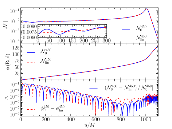
A goal of this paper is to investigate, within the context of characteristic extraction, the effect of the initial data on the calculation of the gravitational news. To this end, we compare waveforms at from two characteristic evolutions based on the same Cauchy boundary data, but different initial data constructions: Jlin-R100-u450 and J0-R100-u450. Both evolutions use boundary data from and begin at the initial time , which was determined above to be a point where the linearized solution is well-matched to the nonlinear evolution. The model Jlin-R100-u450 uses the initial data determined by the linearized solutions, Eqs. (10lnwxakap, 10lnwxakaq). In contrast, J0-R100-u450 simply sets , corresponding to the original prescription of [8, 9]. Fig. 3 plots the Bondi news at as computed from both evolutions, denoted by and for the linearized and initial data runs, respectively. Whereas the phase of shows very little difference between the runs (middle panel), the amplitude shows visible oscillations for the evolution (upper panel and inset). The waveforms agree to within only after a time (which must be added to the starting point of the simulation). Therefore, the influence of the ansatz for the characteristic initial data has a notable impact over an extended time.
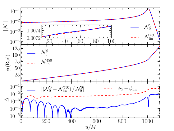
We note, however, that the original prescription of [8, 9] used characteristic initial data at the initial Cauchy time (that is, including the junk radiation). At that time, the shear-free approximation , for the characteristic initial data is compatible with the Cauchy initial data solution.
Hence, we also compare the waveforms of model Jlin-R100-u450 against those of model J0-R100-u0, where the latter model uses initial data at time . The results are plotted in Fig. 4 with the J0-R100-u0 results labeled by . We still observe an oscillation in the amplitude in , though it is drastically reduced compared to the of model J0-R100-u450 shown in Fig. 3. The relative errors in amplitude, plotted in the bottom panel of Fig. 4, are well below over the entire evolution, and the total dephasing is smaller than . We note that the differences are larger than the systematic error reported in [8, 9]. In that work, the error estimate refers to the difference between evolutions starting from the same initial data but different worldtube locations, at a fixed resolution (though the results converge to the same waveform as the resolution is increased). Our results indicate that at typical current resolutions, the choice of characteristic initial data has a larger influence on the simulation error than the worldtube location. The initial burst of junk as well as spurious incoming transients can alter the measured waveforms by an amount that is of the order of the discretization error of current numerical relativity codes (e.g. [27] and references therein), over a period of several hundred .
The numerical tests described so far were with the extraction radius . All these runs were repeated with the extraction radius re-set to . The results are qualitatively similar to the case, and the details are not presented here. One interesting feature was the behaviour of at the worldtube, i.e., the analogy to Fig. 2: it took until about until the decay in the difference between the linearized and actual data was saturated. This is surprising since one would expect that the radiation that passed at about would pass at . One possible explanation is that the saturation is due to nonlinear effects, and since they are somewhat weaker at , saturation takes longer. Furthermore, the boundary data amplitudes are one order of magnitude smaller at than those at , and thus potentially more sensitive to incoming modes. Further studies would be required to fully understand the nature of these effects.
6 Discussion and Conclusion
Characteristic evolutions provide a means of determining radiated gravitational energy which is free from the ambiguities associated with local measures, namely non-linear effects in the near-zone, as well as ambiguities due to gauge and extrapolations to infinity. The principal remaining issue has been to specify appropriate initial data on the null cone, compatible with the data on the worldtube and the Cauchy 3+1 spacetime. The strong correlation between finite radius results and characteristic extraction, as well the invariance of the results on the worldtube location observed in [8, 9] suggests that even the simplest initial data ansatz, , can provide results which are accurate enough for astrophysical estimates, provided the Cauchy 3+1 spacetime is essentially free of radiation at the initial characteristic time. However, in scenarios where strong outgoing radiation is present during the initial characteristic time, data effectively represents incoming radiation, and may alter significantly the evolution of the wave signal towards .
The gravitational wave solution developed in Sec. 3 provides initial data which is compatible, to the linearized level, with outgoing radiation from a binary system. As such, it provides a more physically motivated starting point than the shear-free, , alternative. Importantly, we find that the evolutions which take place from either initialized at a time when outgoing radiation is present at the worldtube, and at the initial time when the Cauchy 3+1 spacetime is conformally flat are very similar (compare Fig. 4), and indeed very similar to the purely 3+1 result which can be obtained by polynomial extrapolating finite radius measurements. That is, for simple choices of initial , the physical conclusions are not altered dramatically, provided the Cauchy 3+1 spacetime does not contain strong amounts of radiation at the worldtube location during the initial characteristic time .
On the other hand, we have demonstrated that the choice of characteristic initial data does result in a small but measurable difference, which decays at a slow exponential rate over a time period of several hundred . We see this transient in the graphs of gravitational news exhibited in Fig. 3. Since the linearized initial data contains only an outgoing mode, we conclude that the shear-free characteristic initial data contains incoming radiation. While this is expected, it is interesting that it takes so much time for the effect to decay away.
This study was designed to assess the long-term effect of characteristic initial data, but it also provides information about the incoming radiation in 3+1 initial data. The point is that the characteristic data on the worldtube is determined entirely by the 3+1 data, and the extent to which this data does not fit the linearized solution is a measure of its incoming radiation content. By construction, the quantities and in the linearized solution must fit the data, with the difference in being an indication of incoming radiation in the 3+1 evolution. Since is not a gauge invariant quantity, it is not possible to make a quantitative statement about the magnitude of the incoming radiation, but Fig. 2 indicates that it takes until at least until it is possible to neglect the effect of incoming radiation in the region .
The effect of incoming radiation in both 3+1 and characteristic initial data decays exponentially, but even so it has a more long-term impact than the outgoing junk radiation which passes the worldtube radius by approximately . The effect of incoming radiation has not received much attention in previous literature dealing with the problem of initial data construction. It has potential significance for the construction of high-accuracy gravitational-wave templates. Further investigations may also explain properties of the incoming radiation content, giving further insight to the peeling property of more complex spacetimes other than Kerr. In particular, it will be important to determine, using a gauge invariant measure, the long-term effect of incoming radiation in 3+1 initial data sets.
The results suggest some promising avenues for future study. Current methods (“characteristic extraction”) transport data in one direction (from the Cauchy to the characteristic code). Great efficiencies would be possible if the coupling were also carried out in the other direction, so that the characteristic evolution would provide outer boundary data for the Cauchy evolution. The linearized wave solution provides a simple recipe for isolating ingoing vs. outgoing modes on the characteristic grid, and may be useful in designing a method for stably transporting data in both directions across the world tube interface.
References
References
- [1] Nigel T. Bishop, Roberto Gómez, Luis Lehner, Manoj Maharaj, and Jeffrey Winicour. Characteristic initial data for a star orbiting a black hole. Phys. Rev. D, 72:024002, 2005.
- [2] Bernard J Kelly, Wolfgang Tichy, Manuela Campanelli, and Bernard F Whiting. Black hole puncture initial data with realistic gravitational wave content. Phys.Rev. D, 76:024008, 2007.
- [3] Ulrich Sperhake. Binary black-hole evolutions of excision and puncture data. Phys.Rev. D, 76:104015, 2007.
- [4] Geoffrey Lovelace. Reducing spurious gravitational radiation in binary-black-hole simulations by using conformally curved initial data. Class. Quantum Grav., 26:114002, 2009.
- [5] N. Bishop, R. Isaacson, R. Gómez, L. Lehner, B. Szilágyi, and J. Winicour. In B. Iyer and B. Bhawal, editors, Black Holes, Gravitational Radiation and the Universe, page 393. Kluwer, Dordrecht, The Neterlands, 1999.
- [6] Maria Babiuc, Belá Szilágyi, Ian Hawke, and Yosef Zlochower. Gravitational wave extraction based on Cauchy-characteristic extraction and characteristic evolution. Class. Quantum Grav., 22:5089–5108, 2005.
- [7] M. C. Babiuc, N. T. Bishop, B. Szilágyi, and Jeffrey Winicour. Strategies for the characteristic extraction of gravitational waveforms. Phys. Rev., D79:084011, 2009.
- [8] C. Reisswig, N. T. Bishop, D. Pollney, and B. Szilagyi. Unambiguous determination of gravitational waveforms from binary black hole mergers. Phys. Rev. Lett., 103:221101, 2009.
- [9] C. Reisswig, N. T. Bishop, D. Pollney, and B. Szilagyi. Characteristic extraction in numerical relativity: binary black hole merger waveforms at null infinity. Class. Quant. Grav., 27:075014, 2010.
- [10] M.C. Babiuc, B. Szilagyi, J. Winicour, and Y. Zlochower. A Characteristic Extraction Tool for Gravitational Waveforms. arXiv:1011.4223, 2010.
- [11] Nigel T. Bishop. Linearized solutions of the Einstein equations within a Bondi-Sachs framework, and implications for boundary conditions in numerical simulations. Class. Quantum Grav., 22(12):2393–2406, 2005.
- [12] H. Bondi, M. G. J. van der Burg, and A. W. K. Metzner. Gravitational waves in general relativity VII. Waves from axi-symmetric isolated systems. Proc. R. Soc. London, A269:21–52, 1962.
- [13] R. Isaacson, J. Welling, and Jeffrey Winicour. Null cone computation of gravitational radiation. J. Math. Phys., 24:1824, 1983.
- [14] N. T. Bishop, R. Gómez, L. Lehner, and J. Winicour. Cauchy-characteristic extraction in numerical relativity. Phys. Rev. D, 54:6153–6165, 1996.
- [15] Nigel T. Bishop, Roberto Gómez, Luis Lehner, Manoj Maharaj, and Jeffrey Winicour. High-powered gravitational news. Phys. Rev. D, 56(10):6298–6309, 15 November 1997.
- [16] R. Gómez. Gravitational waveforms with controlled accuracy. Phys. Rev. D, 64:024007, 2001. gr-qc/0103011.
- [17] Nigel T. Bishop, Roberto Gómez, Luis Lehner, Manoj Maharaj, and Jeffrey Winicour. Incorporation of matter into characteristic numerical relativity. Phys. Rev. D, 60:024005, 1999.
- [18] R.K. Sachs. Gravitational waves in general relativity VIII. Waves in asymptotically flat space-time. Proc. Roy. Soc. London, A270:103–126, 1962.
- [19] Roberto Gómez, Luis Lehner, Philippos Papadopoulos, and Jeffrey Winicour. The eth formalism in numerical relativity. Class. Quantum Grav., 14(4):977–990, 1997.
- [20] Ezra T. Newman and Roger Penrose. Note on the Bondi-Metzner-Sachs group. J. Math. Phys., 7(5):863–870, May 1966.
- [21] J. N. Goldberg, A. J. MacFarlane, Ezra T. Newman, F. Rohrlich, and E. C. G. Sudarshan. Spin- spherical harmonics and . J. Math. Phys., 8(11):2155–2161, 1967.
- [22] Y. Zlochower, R. Gómez, S. Husa, L. Lehner, and J. Winicour. Mode coupling in the nonlinear response of black holes. Phys. Rev. D, 68:084014, 2003.
- [23] Christian Reisswig, Nigel T. Bishop, Chi Wai Lai, Jonathan Thornburg, and Belá Szilágyi. Characteristic evolutions in numerical relativity using six angular patches. Class. Quantum Grav., 24:S327–S339, 2007.
- [24] Charles W. Misner, Kip S. Thorne, and John A. Wheeler. Gravitation. W. H. Freeman, San Francisco, 1973.
- [25] Denis Pollney, Christian Reisswig, Nils Dorband, Erik Schnetter, and Peter Diener. The Asymptotic Falloff of Local Waveform Measurements in Numerical Relativity. Phys. Rev., D80:121502, 2009.
- [26] Denis Pollney, Christian Reisswig, Erik Schnetter, Nils Dorband, and Peter Diener. High accuracy binary black hole simulations with an extended wave zone. arXiv:0910.3803, 2009.
- [27] M. Hannam et al. Samurai project: Verifying the consistency of black-hole-binary waveforms for gravitational-wave detection. Physical Review D, 79(8):084025, April 2009.