0096

WBSDF for Simulating Wave Effects of Light and Audio

1 Supplemental Material

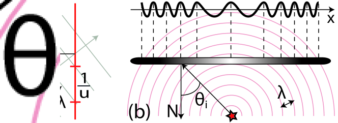
Figure 1: Spatial frequency $u$ of incoming light is dependent on the incident angle $\theta_{i}$ and the wavelength $\lambda$ of the light. The steeper the incoming angle the higher the spatial frequency becomes.

1.1 Hologram recordings

(a) Recording first hologram

(b) Recording hologram with a slit

(c) Recosntruction of the second hologram

Here we present how our BRDF of rainbow holograms, which are found on many credit cards, are computed. The rainbow hologram, invented by Benton Benton1969, is reconstructed by white light and exhibits only the horizontal parallax. The recording process of the rainbow hologram consists of two steps: after the first hologram containing object information is recorded, a horizontal slit is located on top of the first hologram and reconstructed via phase conjugation, and then the second hologram captures the phase conjugated reconstruction from the first hologram [Goodman2005]. The slit allows preserving the horizontal parallax but eliminating color smearing along the vertical direction.

Considering the desired hologram signal, we obtain the WDF of the hologram $\mathcal{W}_{h}$ as

$$\mathcal{W}_{h}(x,u,y,v)=\mathcal{W}_{obj}(x+\lambda_{r}z_{0}u,u,y+\lambda z_{0}(v+v_{0}),v+v_{0})\\ \times\textrm{rect}\left(\frac{v+v_{0}}{A/(z_{A}\lambda_{r})}\right),\qquad\qquad\qquad$$ (1)

where $\mathcal{W}_{obj}$ is the WDF of the object being recorded, $z_{0}$ is the distance between the reconstructed object and the second hologram, $z_{A}$ is the distance between the second hologram and the slit, $\lambda_{r}$ is the recording wavelength, and $v_{0}$ is the spatial frequency along the vertical direction of the reference wave #2.

1.2 Comparison with diffraction shader

Diffraction shaders are very effective in rendering the far field effect of a single bounce. We show that diffraction shader approach is a special case of our method where the light source and a detector (camera) are at infinity. In other words, only the parallel ray bundles are considered. Based on the assumption and equations presented by Stam Stam1999, we present the relationship with WBSDF as follows.

$$I\left(ku^{\prime}\right)=\psi\left(ku^{\prime}\right)\psi\left(ku^{\prime}\right)\\ ~{}\quad=\int\textrm{e}^{ikwh(x)}\textrm{e}^{iku^{\prime}x}\textrm{d}x\int\textrm{e}^{-ikwh(x^{\prime})}\textrm{e}^{-iku^{\prime}x^{\prime}}\textrm{d}x^{\prime}\\ =\iint\textrm{e}^{ikwh(p+\frac{q}{2})}\textrm{e}^{-ikwh(p-\frac{q}{2})}\textrm{e}^{iku^{\prime}q}\textrm{d}p\textrm{d}q~{}~{}\\ =\int\mathcal{W}_{d}(x,u^{\prime})\text{d}x,\qquad\qquad\qquad\qquad\qquad\quad~{}~{}$$ (2)

where $k=2\pi/\lambda$, $u^{\prime}=\sin\theta_{1}-\sin\theta_{2}$, $w=-\cos\theta_{1}-\cos\theta_{2}$, $p=(x+x^{\prime})/2$, $q=x-x^{\prime}$, and $\mathcal{W}_{d}(x,u^{\prime})$ is the WDF of $\text{e}^{ikwh(x)}$ with respect to $\sin\theta_{1}-\sin\theta_{2}$, which represents the reflectance of the surface. In our formulation, as mentioned in Sec. 2.2, the outgoing WDF is written as

$$\mathcal{W}_{2}\left(x,u_{2}\right)=\int\mathcal{W}_{t}\left(x,u_{2};u_{1}\right)\mathcal{W}_{1}\left(x,u_{1}\right)\textrm{d}u_{1}.$$ (3)

Assuming that a plane wave is incident on a surface ($\mathcal{W}_{i}(x,u_{1})=\delta(u_{1}-\sin\theta_{1}/\lambda)$) and a detector is at infinity as in the diffraction shader equations ($u_{2}=\sin\theta_{2}/\lambda$), we obtain the reflected light as

$$I(u_{2})=\int\mathcal{W}_{2}(x,u_{2})\textrm{d}x=\int\mathcal{W}_{t}\left(x,\frac{\sin\theta_{2}}{\lambda};\frac{\sin\theta_{1}}{\lambda}\right)\text{d}x.$$ (4)

Depending on scattering models, various types of $\mathcal{W}_{t}$ are possible. In the diffraction shader, the tangent–plane approximation, where the correlation function depends on both incident and outgoing angles [Hoover2006], has been used, and $\mathcal{W}_{d}(x,\left(\sin\theta_{1}-\sin\theta_{2})/\lambda\right)=\mathcal{W}_{t}\left(x,\sin\theta_{2}/\lambda;\sin\theta_{1}/\lambda\right)$.

If we assume that the angle–shift invariance for further simplification, then the phase function due to a surface can be written as $t_{h}(x)=\textrm{e}^{ik2h(x)}$ and the output WDF is

$$\mathcal{W}_{2}\left(x,u_{2}\right)=\int\mathcal{W}_{t}\left(x,u_{1}\right)\mathcal{W}_{1}\left(x,u_{2}-u_{1}\right)\textrm{d}u_{1}.$$ (5)

If we assume the source and camera at infinities, then

$$I(u_{2})=\int\mathcal{W}_{2}(x,u_{2})\textrm{d}x=\int\mathcal{W}_{t_{h}}(x,u_{2}-u_{1})\textrm{d}x,$$ (6)

where $\mathcal{W}_{t_{h}}$ is the WDF of $\text{e}^{ik2h(x)}$ and this equation is similar to eq. (2). The only difference is that $2h(x)$ and $wh(x)$ in the input functions, where they become identical if we use $\theta_{1}=\theta_{2}=0$. In other words, eq. (6) would produce similar results as the diffraction shader in the paraxial region.

As mentioned in Sec. 2. 2, a statistical model for the phase function can also be applicable to our WDF based method as in the diffraction shader. Contrast to the diffraction shader, we keep the WDF of the surface. Hence, we can use different integration kernels and approximation; e.g., reflection in the near–field can be computed and characteristics of light capturing devices such as cameras can be taken into account in reflection rendering.

For a summary, our approach is more generalized, and different models and approximations, depending on surface profile, light source and camera geometry, speed, tolerance of error, can be incorporated even in the near–field and real camera models.

1.3 Creating BRDFs

1.4 Correlation Function based WBSDF

Based on the generalized van Cittert–Zernike theorem in optics [Goodman2000], the intensity scattered from a surface can be described by the Fourier transform of the coherence factor $\gamma(x,\Delta x)$, which is a normalized correlation function of electric–field ($\langle E(x-\Delta x/2)E^{*}(x+\Delta x/2)\rangle$) at the surface [Wolf1978].

When the exact surface surfaceprofile is unknown, we can derive a WBSDF from the correlation function $\gamma(x,\Delta x)$ of the surface. Where $x$ defines [TC:bla] and $\Delta x$ [TC:bla2]. Since the WDF also can be defined with respect to the correlation function [Bastiaans1997], we can derive the WBSDF from the WDF of the correlation function as

$$\mathcal{W}_{\gamma}(x,u_{o})=\int\gamma(x,\Delta x)\text{e}^{-i2\pi u_{o}\cdot\Delta x}\text{d}\Delta x,$$ (7)

where $u_{o}$ is the local spatial frequency of the outgoing light. If the correlation function depends on the incident light as $\gamma(x,\Delta x;u_{i})$, then we need to compute the WDF for all the incident light as $\mathcal{W}_{\gamma}(x,u_{o};u_{o},u_{i})$. Then the outgoing WDF is expressed as

$$\mathcal{W}_{o}(x,u_{o})=\int\mathcal{W}_{\gamma}(x,u_{o};u_{i})\mathcal{W}_{i}(x,u_{i})\text{d}u_{i}.$$ (8)

Equations (7) and (14) imply that the exact BRDF can be computed provided that the exact surface profile is known. However, it is often challenging to express the exact micro structure. Thus, it is often more convenient to take statistical average of the correlation function, related to parameters such as roughness or periodicity. This approach has been demonstrated in the diffraction shader [Stam1999] and BRDF estimation [Hoover2006].

the statistical properties of the structure to indicate smoothness, periodicity or roughness using an auto-correlation function and standard deviation. Note that WDF is essentially the Fourier transform of the input signals auto-correlation function, so this is highly convenient. Assume we can describe the surface by the autocorrelation function of the surface profile $R_{h}(\Delta x)$ and a standard deviation $\sigma_{h}$. The correlation function can be described by:

$$\gamma(\Delta x)=e^{(i\frac{2\pi}{\lambda}\textrm{sin}\theta_{i}\Delta x)}e^{-\left[\frac{2\pi}{\lambda}\sigma_{h}(1+cos\theta_{i})\right]^{2}+\left[\frac{2\pi}{\lambda}\sigma_{h}(1+cos\theta_{i})\right]^{2}R_{h}(\Delta x)}$$ (9)

Where $\theta_{i}$ is the incident ray angle to the surface normal. We can derive the Wigner Distribution Function for this surface which will give us:

$$I(u) \sim \frac{cos^{2}\theta_{s}}{\lambda^{2}}\int\int\gamma(\Delta x)e^{-ik_{s}\bullet\Delta x}d\Delta x$$ (10)

$$I(u) \sim \frac{cos^{2}\theta_{s}}{\lambda^{2}}e^{-\left[\frac{2\pi}{\lambda}\sigma_{h}(1+cos\theta_{i})\right]^{2}}$$ (12)

$$\Im\left[\left(\frac{2\pi}{\lambda}(1+cos\theta_{i})\right)^{2}R_{h}(\Delta x)\right]|_{\Delta x\rightarrow u-\frac{sin\theta_{i}}{\lambda}}$$

Where $u=\frac{\textrm{sin}\theta_{s}}{\lambda}$.

1.5 Internal reflections

[Are we keeping this section?:]

(d) Internal reflections

(e) Rendering

Figure 2: (a) Shows the principle of internal reflections. Light going out in the same direction are slightly out of phase due to the different travel distances. They end up at the same pixel and create interferences. We can observe this for example when a thin oilfilm is floating on top of water as rendered in (b).

Statistically averaged WBSDF

Equation (6) implies that the BSDF can be computed provided the exact surface profile of the material. However, it is often challenging to express the micro structure exactly. In this situation, we can compute the WBSDF with a statistical average as

$${W}_{t}(x,u)=\int\Big{<}t\left(x+\frac{x^{\prime}}{2}\right)t^{*}\left(x-\frac{x^{\prime}}{2}\right)\Big{>}\text{e}^{-i2\pi x^{\prime}u}\text{d}x^{\prime},$$ (13)

where $\langle~{}\rangle$ denotes average. Depending on the surface properties and rendering environments, different types of statistical average can be used; in general, the Gaussian statistics is assumed and statistics parameters such as standard deviation or autocorrelation length can be tuned. This statistical average approach has been used in the diffraction shader [Stam1999] and BRDF estimation [Hoover2006]. Note that $\langle t\left(x+x^{\prime}/2\right)t^{*}\left(x-x^{\prime}/2\right)\rangle$ is sometimes referred to as the correlation function $\gamma(x,x^{\prime})$. If the correlation function depends on angles of incident and/or outgoing rays, as for example in the diffraction shader, the WDF is expressed as

$${W}_{o}(x,u_{o})=\int{W}_{\gamma}(x,u_{o};u_{i}){W}_{i}(x,u_{i})\text{d}u_{i}.$$ (14)