Trajectories of $L_{4}$ and Lyapunov Characteristic Exponents in the Generalized Photogravitational Chermnykh-Like Problem

Abstract

The dynamical behaviour of near by trajectories is being estimated by Lyapunov Characteristic Exponents(LCEs) in the Generalized Photogravitational Chermnykh-Like problem. It is found that the trajectories of the Lagrangian point $L_{4}$ move along the epicycloid path, and spirally depart from the vicinity of the point. The LCEs remain positive for all the cases and depend on the initial deviation vector as well as renormalization time step. It is noticed that the trajectories are chaotic in nature and the $L_{4}$ is asymptotically stable. The effects of radiation pressure, oblateness and mass of the belt are also examined in the present model.

1 Introduction

In present paper our aim is to obtain trajectories of $L_{4}$ and is to estimate the rate of deviation for initially closely related trajectories in the modified restricted three body problem model(as in Kushvah (2008, 2009a)) with radiation from Sun, oblateness of the second primary(massive body) and influence of the belt. It is supposed that the primary bodies and a belt are moving in a circular orbits about the common center of mass of both primaries. First time such problem was discussed by Chermnykh (1987) and its importance in astronomy has been addressed by Jiang and Yeh (2004a). More generalized cases of the problem were studied by many scientists such as Jiang and Yeh (2004b), Papadakis (2004),Papadakis (2005) and Jiang and Yeh (2006); Yeh and Jiang (2006). The effect of radiation pressure, Poynting-Robertson(P-R)drag and oblateness on the linear stability and nonlinear stability of the $L_{4(5)}$ have been discussed by Kushvah and Ishwar (2006) ; Kushvah et al. (2007a, b, c). In our article Kushvah (2010), we have described the design of the trajectory and analysis of the stability of collinear point $L_{2}$ in the Sun-Earth system.

The first fundamental article about LCN’s was written by Oseledec (1968) in their study of the ergodic theory of dynamical system and Benettin et al. (1980) presented explicit methods for computing all LCEs of a dynamical system. Then Jefferys and Yi (1983) examined stability in the restricted problem of three bodies with Liapunov Characteristic number. First time Wolf et al. (1985) presented an algorithm with FORTRAN code that allows to estimate non-negative Lyapunov Exponents(LEs) from an experimental time series. Sandri (1996) have presented method for numerical calculation of Lyapunov Exponents for a smooth dynamical system with Mathematica[Wolfram (2003)] code. Tancredi et al. (2001) compared two different methods to compute Lyapunov Exponents(LEs). They have shown that since the errors are introduced in the renormalization procedure, it is natural to expect a dependency of the estimated LCEs with the number of renormalization performed in the sense that the smaller the step the worse the estimation. In his study they made conclusion that the two-particle method is not recommended to calculate LCEs in these cases where the solution can fall in a region of regular or quasi regular solution of the phase space. For a region of strong stochastically the LCEs calculated with the two-particle method gives acceptable value.

This paper is organized as follows: In section 2, we state the model of the dynamical system and compute the trajectories of $L_{4}$. Section 3 gives method to compute the LCEs, where subsection 3.1 presents the first order LCEs for various set values of parameters, time ranges and renormalization time steps. Section 4 presents comment about stability using trajectories of $L_{4}$. Lastly, section 5 concludes the paper.

2 Trajectory of $L_{4}$

It is supposed that the motion of an infinitesimal mass particle be influenced by the gravitational force from the two primaries(massive bodies) and a belt of mass $M_{b}$. We also assume that infinitesimal mass does not influence the motion of the two massive bodies which move in circular orbit under their mutual gravitational attraction. Let us assume that $m_{1}$ and $m_{2}$ be the masses of the bigger and smaller primary respectively, $m$ be the mass of the infinitesimal body. The units are normalized by supposing that the sum of the masses to be unity, the distance between both massive bodies to be unity. The rotating frame normalized to rotate with unit angular velocity and the time is normalized in such a way that the time for one period as a unit so that, the Gaussian constant of gravitational $\Bbbk^{2}=1$. For the present model, perturbed mean motion $n$ of the primaries is given by $n^{2}=1+\frac{3A_{2}}{2}+\frac{2M_{b}r_{c}}{\left(r_{c}^{2}+T^{2}\right)^{3/2}}$, where $T=\mathbf{a}+\mathbf{b}$, $\mathbf{a,b}$ are flatness and core parameters respectively[as in Yeh and Jiang (2006)] which determine the density profile of the belt; where $r_{c}^{2}=(1-\mu)q_{1}^{2/3}+\mu^{2}$, $A_{2}=\frac{r^{2}_{e}-r^{2}_{p}}{5r^{2}}$ is the oblateness coefficient of $m_{2}$; $r_{e}$, $r_{p}$ are the equatorial and polar radii of $m_{2}$ respectively, $r$ is the distance between primaries and the radius of the belt; $\mu=\frac{m_{2}}{m_{1}+m_{2}}$ is a mass parameter; $q_{1}=1-\frac{F_{p}}{F_{g}}$ is a mass reduction factor and $F_{p}$ is the solar radiation pressure force which is exactly apposite to the gravitational attraction force $F_{g}$. In a rotating reference frame the coordinates of $m_{1}$ and $m_{2}$ are $(-\mu,0)$ and $(1-\mu,0)$ respectively. We consider the model proposed by Miyamoto and Nagai (1975), and equations of motion are given as in Kushvah (2008) and Kushvah (2009a):

$$\ddot{x}-2n\dot{y} = \Omega_{x},$$ (1)

$$\ddot{y}+2n\dot{x} = \Omega_{y},$$ (2)

where

$$\Omega_{x} = n^{2}x-\frac{(1-\mu)q_{1}(x+\mu)}{r^{3}_{1}}-\frac{\mu(x+\mu-1)}{r^{3}_{2}}-\frac{3}{2}\frac{\mu{A_{2}}(x+\mu-1)}{r^{5}_{2}}$$

$$-\frac{M_{b}x}{\left(r^{2}+T^{2}\right)^{3/2}}-\frac{W_{1}}{r^{2}_{1}}\biggl{[}\frac{(x+\mu)}{r^{2}_{1}}\{(x+\mu){\dot{x}+y\dot{y}}\}+\dot{x}-ny\biggr{]},$$

$$\Omega_{y} = n^{2}y-\frac{(1-\mu)q_{1}{y}}{r^{3}_{1}}-\frac{\mu{y}}{r^{3}_{2}}-\frac{3}{2}\frac{\mu{A_{2}}y}{r^{5}_{2}}$$

$$-\frac{M_{b}y}{\left(r^{2}+T^{2}\right)^{3/2}}-\frac{W_{1}}{r^{2}_{1}}\biggl{[}\frac{y}{r^{2}_{1}}\{(x+\mu)\dot{x}+y\dot{y}\}+\dot{y}+n(x+\mu)\biggr{]},$$

$$\Omega = \frac{n^{2}(x^{2}+y^{2})}{2}+\frac{(1-\mu)q_{1}}{r_{1}}+\frac{\mu}{r_{2}}+\frac{\mu A_{2}}{2r_{2}^{3}}+\frac{M_{b}}{\left(r^{2}+T^{2}\right)^{1/2}}$$

$$+W_{1}\left\{\frac{(x+\mu)\dot{x}+y\dot{y}}{2r_{1}^{2}}-n\arctan\left(\frac{y}{x+\mu}\right)\right\},$$

$$W_{1} = \frac{(1-\mu)(1-q_{1})}{c_{d}},\ r_{1}^{2}=(x+\mu)^{2}+y^{2},\ r_{2}^{2}=(x+\mu-1)^{2}+y^{2}.$$

The parameter $W_{1}$ is considered due to P-R drag[more review in Poynting (1903),Robertson (1937), Chernikov (1970), Murray (1994) and Kushvah (2009b)]. Where $r_{1}$, $r_{2}$ are the distances of $m$ from first and second primary respectively. The dimensionless velocity of the light is supposed to be $c_{d}=299792458$. Then from equations (1) and (2) energy integral is given as:

$$E=\frac{1}{2}\left(\dot{x}^{2}+\dot{y}^{2}\right)-\Omega(x,y,\dot{x},\dot{y})=(\mbox{Constant})$$ (3)

where the quantity $E$ is an energy integral related to the Jacobi’s constant $C(=-2E)$.

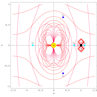
For numerical computation of equilibrium points, we divide the orbital plane $Oxy$ into three parts $x\leq-\mu$, $-\mu<x<1-\mu$ and $1-\mu\leq x$ with respect to the primaries. For the simplicity, we set $\mu=9.537\times 10^{-4},T=0.01$. The equilibrium points are given by substituting $\Omega_{x}=\Omega_{y}=0$, and presented in figure 1 when $q_{1}=0.75$, $A_{2}=0.25$, $M_{b}=0.25$. In this figure the dark blue dotes present the position of $L_{4}(5):(x=0.347988,y=\pm 0.70645)$, the light blue represent the collinear equilibrium points $L_{1}:x=0.753578,L_{2}:x=1.14795$ and $L_{3}:x=-0.788385$ for which $y=0$.

Figure 1: The position of equilibrium points.

The equations (1-2) with initial conditions $x(0)=\frac{1-2\mu}{2}$, $y(0)=\frac{\sqrt{3}}{2}$, $x^{\prime}(0)=y^{\prime}(0)=0$ are used to determine the trajectories of $L_{4}$ for different possible cases. At at time $t=0$, the origin of coordinate axes is supposed at the equilibrium point.

Figure 2: Trajectory of $L_{4}$ when $q_{1}=0.75,A_{2}=0.0$ in frame(a) blue curve for $0\leq t\leq 50$, (b) red for $50\leq t\leq 100$ and (c) green for $0\leq t\leq 200$. Frames(a-c) $M_{b}=0.0$, and frames (d-f) $M_{b}=0.25$.

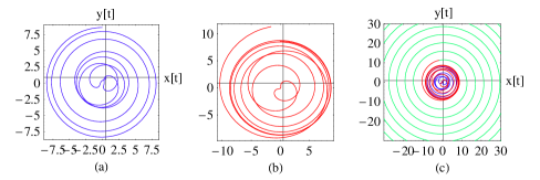
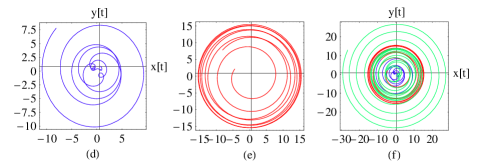
In the present model all the computed trajectories of the $L_{4}$ follow approximately the same path described by an epitrochoid whose parametric equations are given as:

$$x(t) = (a_{1}+b_{1})\cos t-d_{1}\cos\left(\frac{a_{1}+b_{1}}{b_{1}}t\right)$$ (4)

$$y(t) = (a_{1}+b_{1})\sin t-d_{1}\sin\left(\frac{a_{1}+b_{1}}{b_{1}}t\right)$$ (5)

where $a_{1}$ is radius of a fixed circle, $b_{1}$ is radius of rolling circle and $d_{1}$ is distance form center of rolling circle to to the point$(x(t),y(t))$ which forms a trajectory. It is evident from above equations that if $d_{1}$ depends on time then orbit is unstable and trajectory moves spirally outward the vicinity of the initial point.

When $q_{1}=0.75,A_{2}=0$, the trajectory is shown in figure 2 with panels(a-d) for $M_{b}=0.0$ and panels(e-f) for $M_{b}=0.0$, where frames(a& d) $0\leq t\leq 50$, (b&e) $50\leq t\leq 100$ and (c&f) $0\leq t\leq 200$. It is clear from figure that if $0\leq t\leq 50$ and $M_{b}=0.0$ the trajectory of $L_{4}$ is similar to the curve described by epitrochoid (4, 5) for $a_{1}=1/7,b_{1}=1=d_{1}$. When $t>50$ then $d_{1}$ becomes function of time $t$, and the trajectory moves spirally outward. When $M_{b}=0.25$, the trajectory follows the path correspond to parameters $a_{1}=1,b_{1}=\sqrt{5}$(irrational), $d_{1}=3$. Here the value of $b_{1}$ is irrational number which shows that the motion is non periodic.

Figure 3: Trajectory of $L_{4}$ when $q_{1}=0.75,M_{b}=0.25$, where frames(a-c) for $A_{2}=0.25$ and frames(d-f) for $A_{2}=0.50$.

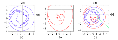
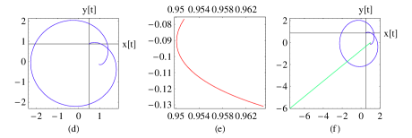
When $q_{1}=0.75,M_{b}=0.25$, figure 3 depicts the trajectory for $L_{4}$ with frames(a-c) for $A_{2}=0.25$ and frames(d-f) for $A_{2}=0.50$. In frame(a) $0\leq t\leq 50$, (b) $50\leq t\leq 75$ and (c) $0\leq t\leq 77$ while (d) $0\leq t\leq 8.2$, (e) $8.2\leq t\leq 8.3$ and (f)$0\leq t\leq 9$. It is clear from frames(a-c) that the trajectory moves along approximately epicycloid path, when $t$ increases it departs form the vicinity of $L_{4}$. The region of stability shrinks and trajectory moves along a single cusped epicycloid, then it departs far from the initial point. Hence oblateness effect is significant factor to reducing the stability region.

3 Lyapunov Characteristic Exponents(LCEs)

It is well known that, if LCE$>0$ for some initial conditions which indicates the trajectory of initial condition is unstable. If LCE$=0$ for some values of initial conditions the orbit is neutrally stable and which corresponds to regular motion. If LCE$<0$, the corresponding orbit is asymptotically stable. Now suppose $S$ be a 4-dimensional phase space such that $S=\{X:X=[x(t),y(t),p_{x}(t),p_{y}(t)]^{Tran}\}$ , then the time evaluation of the orbit is governed by the equation

$$\dot{X}=f(X)=\left[\frac{\partial{H}}{\partial{x}}\ \frac{\partial{H}}{\partial{y}}\ -\frac{\partial{H}}{\partial{p_{x}}}\ -\frac{\partial{H}}{\partial{p_{y}}}\right]^{tran}=J_{4}DHX$$ (6)

where $D=\frac{\partial{}}{\partial{X}}$ and

$$J_{4}=\begin{bmatrix}0&0&1&0\\ -1&0&0&1\\ 0&-1&0&0\end{bmatrix}.$$ (7)

The dynamical system is described by the Hamiltonian $H$ which depends on Jacobian constant and given by

$$H=\frac{1}{2}\left(p_{x}^{2}+p_{y}^{2}\right)+n(yp_{x}-xp_{y})-U(x,y)$$ (8)

where $p_{x},p_{y}$ are the momenta coordinates given by

$$\dot{p_{x}}=-\frac{\partial{H}}{\partial{p_{x}}},\ \dot{p_{y}}=-\frac{\partial{H}}{\partial{p_{y}}},$$

$$U(x,y)=\Omega-\frac{n^{2}(x^{2}+y^{2})}{2},$$

Consider $v=(\delta{x},\delta{y},\delta{p_{x}},\delta{p_{y}})$ be a deviation vector from initial condition $X(0)$ such that $||v_{0}||=1$. Then the variational equation is given

$$\dot{v}=Df(X).v$$ (9)

$$\mbox{or}\quad\begin{bmatrix}\delta\dot{x}\\ \delta\dot{y}\\ \delta\dot{p_{x}}\\ \delta\dot{p_{y}}\end{bmatrix}=\begin{bmatrix}0&n&1&0\\ -n&0&0&1\\ U^{t}_{xx}&U^{t}_{xy}&0&n\\ U^{t}_{yx}&U^{t}_{yy}&-n&0\end{bmatrix}\begin{bmatrix}\delta{x}\\ \delta{y}\\ \delta{p_{x}}\\ \delta{p_{y}}\end{bmatrix},$$ (10)

where superscript $t$ over partial derivatives of $U$ indicates their respective values at $t$ etc. Then the Lyapunov Characteristic Exponent is given by

$$\lambda(v(t))=\lim_{t->\infty}\log\frac{||v(t)||}{||v(0||}.$$ (11)

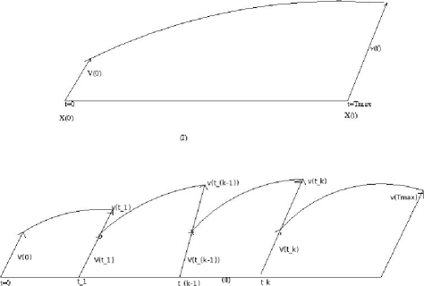
For numerical computation of LCEs we use method presented in Skokos and Gerlach (2010) and Skokos (2010). To avoid overflow in numerical computation, we partition the closed interval $I=[t_{0},Tmax]$ into $n_{1}$ sub intervals with time step $\Delta t$ and the time to run from $0$ to $Tmax$ i.e.

$$P(I)=\left\{0=t_{0},t_{1},t_{2},t_{3},\dots t_{k-1},t_{k},\dots,t_{n_{1}}=Tmax\right\},$$ (12)

then equation (11) can be written as

$$\lambda(v(t))=\lim_{{n_{1}}t->\infty}\sum_{k=0}^{n_{1}}{\log\alpha(t_{k})},$$ (13)

where $\alpha(t_{k})=||v(t_{k})||$. To determine first order LCEs in next section, we will use initial vector $X(0)=(0.499046,0.866025,-0.866025,0.499046)$ for classical RTBP($q_{1}=1,A_{2}=0,M_{b}=0$) and $X(0)=(0.337957,0.81415,-0.954676,0.39629)$ for modified RTBP( $q_{1}=0.75,A_{2}=0.25,M_{b}=0.25$). As in figure 4, at each step $v(t_{k})$ will be evaluated from (6,10) using $X(t_{k-1})$ and unit deviation vector $\hat{v}(t_{k-1})=V(t_{k-1})$(say).

Figure 4: In Plot (I) only one step is used to obtain LCEs while in (II) more that one normalization steps are used and $V(t_{k-1})$ denotes the unit deviation vector for all $k$.

3.1 First Order LCEs

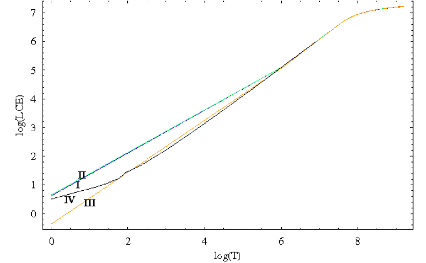
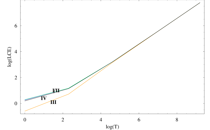
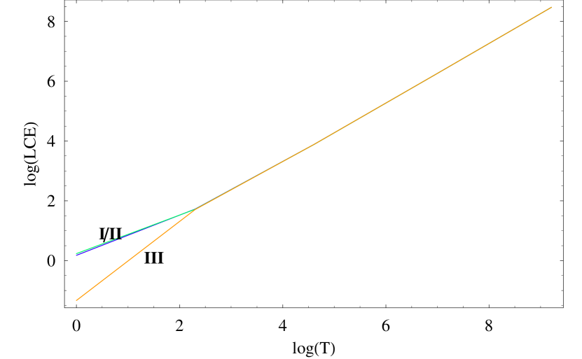
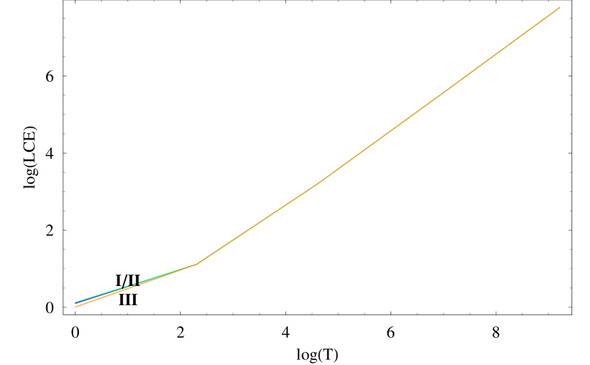
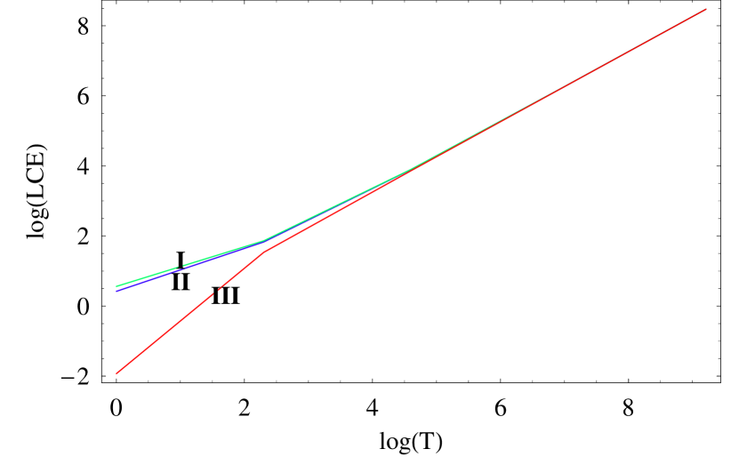
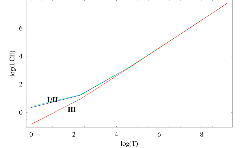
Now consider $R^{4}=LD_{1}$, $R^{3}=LD_{2}$, $R^{2}=LD_{3}$ and $R^{1}=LD_{4}$ spaces such that $LD_{1}\supset LD_{2}\supset LD_{3}\supset LD_{4}$. To find the first order LCE($\lambda_{i}),(i=1,2,3,4)$, we choose initial unit deviation vectors from $LD_{1}\backslash LD_{2}$: $v_{11}=(1/2,1/2,1/2,1/2)$, $v_{12}=(0,\frac{1}{\sqrt{3}},\frac{1}{\sqrt{3}},\frac{1}{\sqrt{3}})$, $v_{13}=(0,0,\frac{1}{\sqrt{2}},\frac{1}{\sqrt{2}})$, $v_{14}=(0,0,0,1)$. The values of LCEs are presented in log-log plot figure 5 for $t=0-10000$ when $q_{1}=0.75,A_{2}=0.25,M_{b}=0.25$ left panel corresponding to $\Delta t=1$ and right for $\Delta t=2$. Initially the values of LCE($\lambda_{1}$) are different, they are shown by curves(I)-(IV) correspond to four vectors respectively, but when $t$ increases they merge into a single curve. To obtain LCE($\lambda_{2}$), we choose initial unit deviation vectors from $LD_{2}\backslash LD_{3}$ such that $v_{21}=(\frac{1}{\sqrt{3}},\frac{1}{\sqrt{3}},\frac{1}{\sqrt{3}},0)$, $v_{22}=(0,\frac{1}{\sqrt{2}},\frac{1}{\sqrt{2}},0)$, $v_{23}=(0,0,1,0)$. Figure 6 shows LCE($\lambda_{2}$) when $q_{1}=0.75,A_{2}=0.25,M_{b}=0.25$, where left panel corresponds to $\Delta t=1$ and right for $\Delta t=2$.

Figure 5: LCE$(\lambda_{1})$ when $q_{1}=0.75,A_{2}=0.25,M_{b}=0.25$ and $0\leq t\leq 10000$; curve (I) $v_{11}=(1/2,1/2,1/2,1/2)$,(II):$v_{12}=(0,\frac{1}{\sqrt{3}},\frac{1}{\sqrt{3}},\frac{1}{\sqrt{3}})$, (III):$v_{13}=(0,0,\frac{1}{\sqrt{2}},\frac{1}{\sqrt{2}})$ and (IV):$v_{14}=(0,0,0,1).$

Figure 6: LCE$(\lambda_{2})$ when $q_{1}=0.75,A_{2}=0.25,M_{b}=0.25$ and $0\leq t\leq 10000$; curves (I) $v_{21}=(\frac{1}{\sqrt{3}},\frac{1}{\sqrt{3}},\frac{1}{\sqrt{3}},0)$,(II):$v_{22}=(0,\frac{1}{\sqrt{2}},\frac{1}{\sqrt{2}},0)$ and (III):$v_{23}=(0,0,1,0).$

Figure 7: LCEs when $0\leq t\leq 10000$, $q_{1}=0.75,A_{2}=0.25$ and $M_{b}=0.25$; where LCE$(\lambda_{3})$:(I) $v_{31}=(\frac{1}{\sqrt{2}},\frac{1}{\sqrt{2}},0,0)$,(II):$v_{32}=(0,1,0,0)$ and LCE$(\lambda_{4})$(III):$v_{41}=(1,0,0,0).$

Figure 8: LCE$(\lambda_{2})$ when $q_{1}=1,A_{2}=0,M_{b}=0$ and $0\leq t\leq 100$; where (I):$v_{21}=(\frac{1}{\sqrt{3}},\frac{1}{\sqrt{3}},\frac{1}{\sqrt{3}},0)$,(II):$v_{22}=(0,\frac{1}{\sqrt{2}},\frac{1}{\sqrt{2}},0)$ and (III):$v_{23}=(0,0,1,0).$

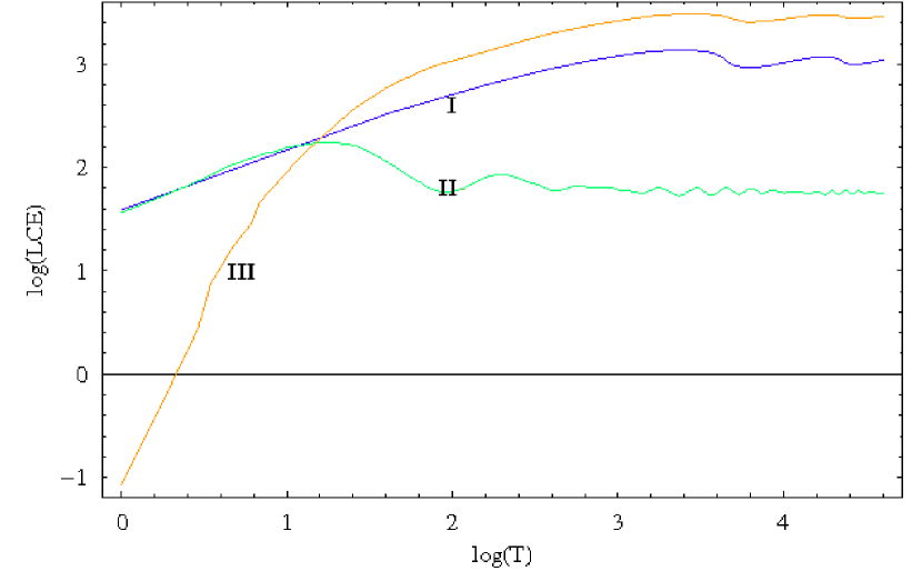
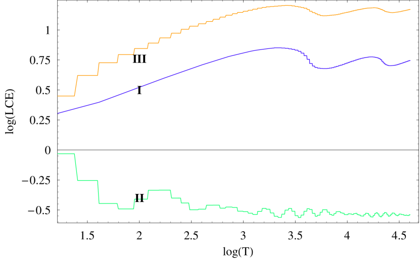
Now for computation of LCE($\lambda_{3}$), we choose initial unit deviation vectors from $LD_{3}\backslash LD_{4}$. The results are presented in figure 7 for $q_{1}=0.75,A_{2}=0.25,M_{b}=0.25$ and $0\leq t\leq 10000$ with left frame for $\Delta t=1$ and right for $\Delta t=2$. In figures 8 and 9, curves are plotted when $q_{1}=1,A_{2}=0,M_{b}=0$, where left panel corresponding to $\Delta t=0.1$ and right for $\Delta t=1$. In figure 8, curves are labeled as(I) $v_{21}=(\frac{1}{\sqrt{3}},\frac{1}{\sqrt{3}},\frac{1}{\sqrt{3}},0)$,(II):$v_{22}=(0,\frac{1}{\sqrt{2}},\frac{1}{\sqrt{2}},0)$, (III):$v_{23}=(0,0,1,0)$ and in figure 9, curves are plotted for $0\leq t\leq 100$, where (I) $v_{31}=(\frac{1}{\sqrt{2}},\frac{1}{\sqrt{2}},0,0)$,(II):$v_{32}=(0,1,0,0)$. The curves are in wave form with decreasing amplitudes which tend to zero at infinity and curves become constant.

Figure 9: LCE$(\lambda_{3})$ when $q_{1}=1,A_{2}=0,M_{b}=0$ and $0\leq t\leq 100$; where (I):$v_{31}=(\frac{1}{\sqrt{2}},\frac{1}{\sqrt{2}},0,0)$ and (II):$v_{32}=(0,1,0,0)$.

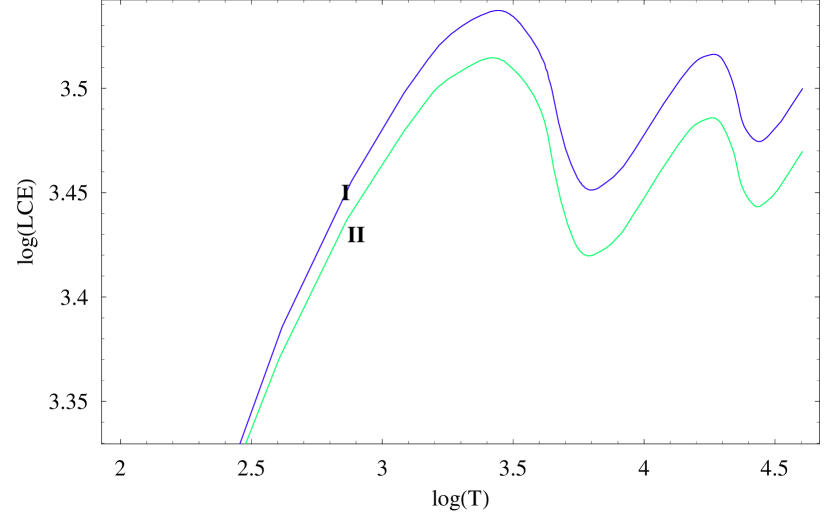
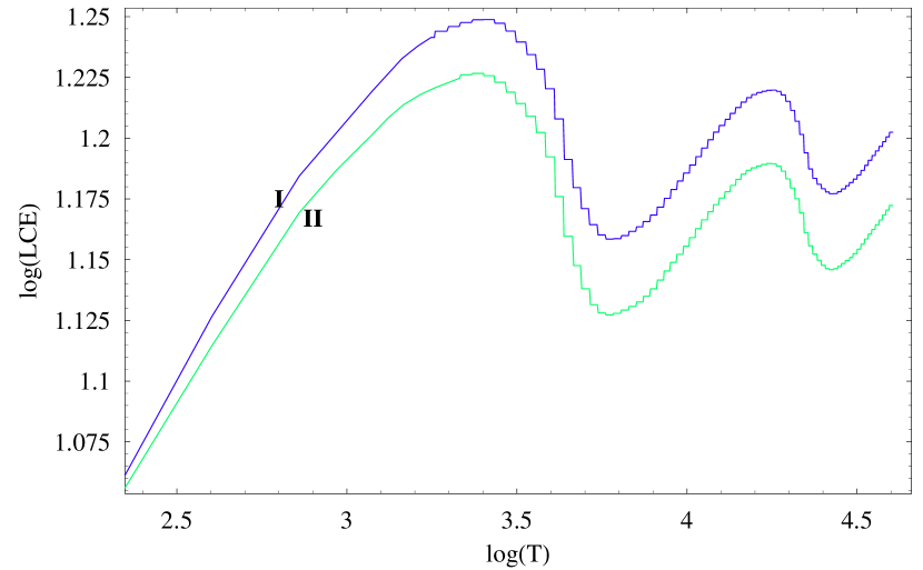
To determine LCE$(\lambda_{4})$, we choose $v_{41}=(1,0,0,0)$ from $LD_{4}$ . The corresponding LCE is shown by curve (III) in figure 7:$q_{1}=0.75,A_{2}=0.25,M_{b}=0.25$ with left frame for $\Delta t=1$ and right for $\Delta t=2$. In figure 10, we consider $q_{1}=1,A_{2}=0.0,M_{b}=0.0$ in which curve(I) represents renormalization time step $\Delta t=0.1$ and (II) for $\Delta t=1$. It can be seen that (I) is a smooth curve and (II) is initially stepped curve but both curves are initially increasing in nature and after certain time they become constant.

Figure 10: LCE$(\lambda_{4})$ when $q_{1}=1,A_{2}=0.0,M_{b}=0.0$ and $v_{41}=(1,0,0,0)$ where curve(I) represents the renormalization time step $\Delta t=0.1$ and (II) for $\Delta t=1$.

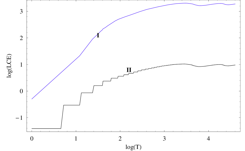
The LCEs$(\lambda_{i}),(i=1,2,3,4)$ are presented in Table 1 for initial point $X(0)=(0.337957,0.81415,-0.954676,0.39629)$ and $q_{1}=0.75,A_{2}=0.25,M_{b}=0.25.$ It is clear from figures and Table that all first order LCEs are positive for various set values of parameters and renormalization time steps. This shows that the present dynamical system is stochastic. It is also noticed that if $Tmax$ is not very large the LCEs depend on the choice of the renormalization time step as well as initial deviation vectors while if $Tmax$ is very large then LCEs depend on renormalization time step only.

Table 1: First order LCEs for initial point $X(0)=(0.337957,0.81415,-0.954676,0.39629)$ when $q_{1}=0.75,A_{2}=0.25,M_{b}=0.25.$

$\log t$	$\log{\lambda_{1}(v_{11})}$	$\log{\lambda_{1}(v_{12})}$	$\log{\lambda_{1}(v_{13})}$	$\log{\lambda_{1}(v_{14})}$	$\log{\lambda_{2}(v_{21})}$	$\log{\lambda_{2}(v_{22})}$	$\log{\lambda_{2}(v_{23})}$	$\log{\lambda_{3}(v_{31})}$	$\log{\lambda_{3}(v_{32})}$	$\log{\lambda_{4}(v_{41})}$
					$\Delta t=1$
$\log 10^{0}$	0.403836	0.446978	-0.474575	0.182934	0.176488	0.233361	-1.33349	0.420617	0.561358	-1.92815
$\log 10^{1}$	1.78922	1.79078	1.31139	1.75423	1.72431	1.71777	1.70948	1.83046	1.86196	1.53422
$\log 10^{2}$	3.89211	3.89209	3.83842	3.88798	3.88433	3.88314	3.88489	3.89796	3.90179	3.8656
$\log 10^{3}$	6.17181	6.17188	6.16639	6.17139	6.17102	6.17098	6.1711	6.17242	6.17281	6.16922
$\log 10^{4}$	8.47207	8.47216	8.47153	8.47203	8.47199	8.47208	8.472	8.47213	8.47217	8.47188
					$\Delta t=2$
$\log 10^{0}$	0.266298	0.287879	-0.594977	0.195472	0.101962	0.124369	0.00722875	0.335259	0.418618	-0.849014
$\log 10^{1}$	1.17546	1.17649	0.719618	1.1448	1.11437	1.10752	1.11319	1.21633	1.24543	0.936813
$\log 10^{2}$	3.2087	3.20867	3.15533	3.20463	3.20098	3.19979	3.20168	3.21453	3.21832	3.18239
$\log 10^{3}$	5.47966	5.47973	5.47424	5.47924	5.47887	5.47883	5.47895	5.48027	5.48066	5.47707
$\log 10^{4}$	7.77903	7.77911	7.77848	7.77898	7.77895	7.77903	7.77895	7.77909	7.77913	7.77884
					$\Delta t=10$
$\log 10^{1}$	0.030892	0.030311	-0.25883	0.011177	-0.0066539	-0.013192	-0.002721	0.0587713	0.076341	-0.10142
$\log 10^{2}$	1.67368	1.67363	1.6238	1.66989	1.66652	1.66538	1.66726	1.67913	1.68263	1.64948
$\log 10^{3}$	3.87816	3.87824	3.87278	3.87775	3.87738	3.87734	3.87746	3.87877	3.87915	3.87559
$\log 10^{4}$	6.17039	6.17047	6.16985	6.17035	6.17031	6.17039	6.17032	6.17045	6.17049	6.1702
					$\Delta t=100$
$\log 10^{2}$	-0.0374842	-0.0374685	-0.064786	-0.039577	-0.0414376	-0.042026	-0.0410299	-0.0344616	-0.0325176	-0.0507718
$\log 10^{3}$	1.66081	1.66088	1.65587	1.66043	1.66009	1.66006	1.66016	1.66136	1.66172	1.65846
$\log 10^{4}$	3.87675	3.87684	3.87621	3.87671	3.87667	3.87676	3.87668	3.87681	3.87685	3.87657
					$\Delta t=1000$
$\log 10^{3}$	1.66081	1.66088	1.65587	1.66043	1.66009	1.66006	1.66016	1.66136	1.66172	1.65846
$\log 10^{4}$	3.87675	3.87684	3.87621	3.87671	3.87667	3.87676	3.87668	3.87681	3.87685	3.87657
					$\Delta t=10000$
$\log 10^{4}$	-0.0452992	-0.0452123	-0.0455707	-0.0453203	-0.045339	-0.0452492	-0.0453349	-0.0452687	-0.045249	-0.0453539

Note. — The values of LCEs depend on time step for normalization more than the initial deviation vector.

4 Stability of $L_{4}$

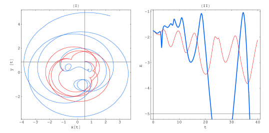
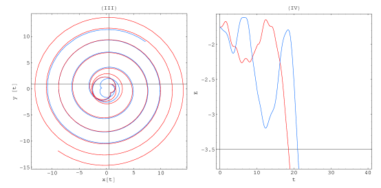
Now we suppose that the coordinates $(x_{1},y_{1})$ of $L_{4}$ are initially perturbed by changing $x(0)=x_{1}+\epsilon\cos(\phi),y(0)=y_{1}+\epsilon\sin(\phi)$ where $\phi=\arctan\left(\frac{y(0)-y_{1}}{x(0)-x_{1}}\right)\in(0,2\pi),0\leq\epsilon<1$; $\phi$ indicates the direction of the initial position vector in the local frame. For simplicity, it is supposed that $\epsilon=0.001$ and $\phi=\frac{\pi}{4}$. We solved (1, 2) numerically using above perturbed initial point and plotted figure 11 when $A_{2}=0.0$, which shows that the orbit of test particle and its energy constant. When $q_{1}=0.75$ we have panels(I&II) and $q_{1}=0.50$ then (III&IV) in which (I&III) describe the trajectory and (II&IV) correspond to energy integral $E$. It is clear from the orbit that initially trajectory moves in epicycloid path described by (4, 5) without deviating far from $L_{4}$ and energy constant remains negative; but after a certain time it moves spirally outward from the region and energy constant becomes positive. Here blue curves represent $M_{b}=0.25$ and red curves correspond to $M_{b}=0.50$.

Figure 11: Stability of $L_{4}$ when $A_{2}=0.0$ with panels (I&II):$q_{1}=0.75$ and (III&IV):$q_{1}=0.50$ in which blue curves correspond to $M_{b}=0.25$ and red for $M_{b}=0.50$.

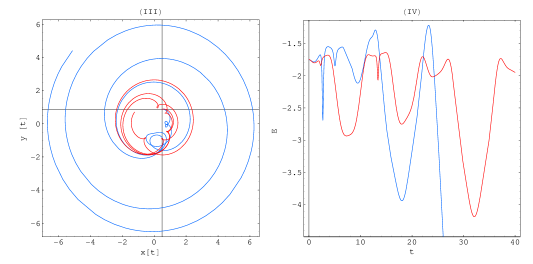
The effect of oblateness of the second primary is shown in figure 12 when $M_{b}=0.25$, where (I&II) correspond to $q_{1}=0.75$ and (III&IV) for $q_{1}=0.50$. Panels (I& III) show the trajectory of perturbed point $L_{4}$ and (II&IV) describe the energy integral of that point. The blue curves correspond to $A_{2}=0.25$ and red for $A_{2}=0.50$. The trajectory of perturbed point follows the path described by epitrochoid (4,5), as time increases it moves spirally outward from the vicinity of $L_{4}$. It is seen that the oblateness is a significant effect on the trajectory and the stability of $L_{4}$. When $A_{2}=0.0$ the $L_{4}$ is asymptotically stable for the value of $t$ which lies within a certain interval. But if oblate effect of second primary is present($A_{2}\neq 0$), the stability region of $L_{4}$ disappears for large values of $A_{2}$.

Figure 12: Effect of oblateness on the stability of $L_{4}$ when $M_{b}=0.25$ panels (I&II)$q_{1}=0.75$ (III&IV) $q_{1}=0.50$ in which blue solid curves for $A_{2}=0.25$, red curves for $A_{2}=0.50$.

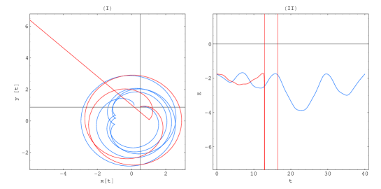
From relation $A_{2}=\frac{r^{2}_{e}-r^{2}_{p}}{5r^{2}}$ we obtain $\frac{r_{e}}{r}=\sqrt{5A_{2}+\frac{r_{p}}{r}}$. This shows that if $A_{2}$ increases means the ratio $\frac{r_{e}}{r}$ increases consequently $\frac{r_{e}}{r_{1}}$ increases. Then form Ryabov and Yankovsky (2006), it is found that as the attracting particle recedes that is the ratio $\frac{r_{e}}{r_{1}}$ diminishes, the difference between the attraction of spheroid and that of a sphere will decrease and, if $r$(or $r_{1}$) is very large in comparison with $r_{e}$, the spheroid will exert a force that practically coincided with that of a sphere. If $A_{2}=0.5$ i.e. very large value then $r_{e}>r$(hypothetically) then second primary becomes a thin flat disk. In this case the both primaries have no separate gravitational attraction so they act like a single body and its sphere of influence is common with very large radius, that attracts perturbed point. Since perturbed point $L_{4}$ is supposed in the equatorial plane of second primary, so the attraction of the oblate spheroid(equatorial bulge) upon $L_{4}$ at a given distance from the centre of primary is greater than that of a sphere of equal mass($A_{2}=0.0$) which has been proved by Moulton (1960). The effect of oblateness can be seen in frame(c) of figure 2 and in frame(I) of figure 12, where attraction of the equatorial bulge of the second primary increases with $A_{2}$. Hence from above discussion we can say that if $A_{2}=0.50$(hypothetically), the trajectory suddenly moves from the vicinity of $L_{4}$ as the time increase.

5 Conclusion

We have obtained the trajectories of $L_{4}$ and its perturbed point, for various set values of parameters. It is found that the trajectories move along the epicycloid path upto a certain time then they move spirally outward from the vicinity of the point. From the first order Lyapunov Characteristic Exponents(LCEs), we have seen that the behaviours of trajectories are stochastic. It is also found that the radiation pressure, mass of the belt and oblateness are significant effects, they reduce the stability region and increase the stochasticity in the system. It is also found that if $A_{2}=0.50$(hypothetically), the trajectory suddenly moves from the vicinity of $L_{4}$ as the time increase.

References

- Benettin et al. (1980) Benettin, G., Galgani, L., Giorgilli, A., Strelcyn, J., Mar. 1980. Lyapunov characteristic exponents for smooth dynamical systems and for Hamiltonian systems - A method for computing all of them. I - Theory. II - Numerical application. Meccanica 15, 9–30.
- Chermnykh (1987) Chermnykh, S. V., 1987. Stability of libration points in a gravitational field. Vest. Leningrad Mat. Astron. 2, 73–77.
- Chernikov (1970) Chernikov, Y. A., Feb. 1970. The photogravitational restricted three-body problem. AZh47, 217.
- Jefferys and Yi (1983) Jefferys, W. H., Yi, Z., May 1983. Stability in the restricted problem of three bodies with Liapounov Characteristic Numbers. Celestial Mechanics 30, 85–95.
- Jiang and Yeh (2004a) Jiang, I., Yeh, L., Sep. 2004a. Dynamical Effects from Asteroid Belts for Planetary Systems. International Journal of Bifurcation and Chaos 14, 3153–3166.
- Jiang and Yeh (2004b) Jiang, I.-G., Yeh, L.-C., Aug. 2004b. On the Chaotic Orbits of Disk-Star-Planet Systems. AJ128, 923–932.
- Jiang and Yeh (2006) Jiang, I.-G., Yeh, L.-C., Dec. 2006. On the Chermnykh-Like Problems: I. the Mass Parameter = 0.5. Ap&SS305, 341–348.
- Kushvah (2008) Kushvah, B. S., Jun. 2008. The effect of radiation pressure on the equilibrium points in the generalized photogravitational restricted three body problem. Ap&SS315, 231–241.
- Kushvah (2009a) Kushvah, B. S., Sep. 2009a. Linearization of the Hamiltonian in the generalized photogravitational Chermnykh’s problem. Ap&SS323, 57–63.
- Kushvah (2009b) Kushvah, B. S., Sep. 2009b. Poynting-Robertson effect on the linear stability of equilibrium points in the generalized photogravitational Chermnykh’s problem. Research in Astronomy and Astrophysics 9, 1049–1060.
- Kushvah (2010) Kushvah, B. S., Oct. 2010. Trajectory and stability of Lagrangian point in the Sun-Earth system. Ap&SS, 286–+.
- Kushvah and Ishwar (2006) Kushvah, B. S., Ishwar, B., 2006. Linear stability of triangular equilibrium points in the generalized photogravitational restricted three body problem with Poynting-Robertson drag. Journal of Dynamical Systems & Geometric Theories 4(1), 79–86.
- Kushvah et al. (2007a) Kushvah, B. S., Sharma, J. P., Ishwar, B., 2007a. Higher order normalizations in the generalized photogravitational restricted three body problem with Poynting-Robertson drag. Bulletin of the Astronomical Society of India 35, 319–338.
- Kushvah et al. (2007b) Kushvah, B. S., Sharma, J. P., Ishwar, B., Dec. 2007b. Nonlinear stability in the generalised photogravitational restricted three body problem with Poynting-Robertson drag. Ap&SS312, 279–293.
- Kushvah et al. (2007c) Kushvah, B. S., Sharma, J. P., Ishwar, B., Oct. 2007c. Normalization of Hamiltonian in the Generalized Photogravitational Restricted Three Body Problem with Poynting Robertson Drag. Earth Moon and Planets 101, 55–64.
- Miyamoto and Nagai (1975) Miyamoto, M., Nagai, R., 1975. Three-dimensional models for the distribution of mass in galaxies. PASJ27, 533–543.
- Moulton (1960) Moulton, F. R., 1960. An Introduction to Celestial Mechanics, second revised Edition. The Macmillan Company.
- Murray (1994) Murray, C. D., Dec. 1994. Dynamical effects of drag in th circular restricted three-body problem. 1: Location and stability of the Lagrangian equilibrium points. Icarus 112, 465–484.
- Oseledec (1968) Oseledec, V., 1968. A multiplicative ergodic theorem, Lyapunov characteristic numbers for dynamical systems. Transactions of Moscow Mathematics Society 19, 197–231.
- Papadakis (2004) Papadakis, K. E., Oct. 2004. The 3D restricted three-body problem under angular velocity variation. A&A425, 1133–1142.
- Papadakis (2005) Papadakis, K. E., Sep. 2005. Motion Around The Triangular Equilibrium Points Of The Restricted Three-Body Problem Under Angular Velocity Variation. Ap&SS299, 129–148.
- Poynting (1903) Poynting, J. H., Nov. 1903. Radiation in the solar system : its effect on temperature and its pressure on small bodies. MNRAS64, 525–552.
- Robertson (1937) Robertson, H. P., Apr. 1937. Dynamical effects of radiation in the solar system. MNRAS97, 423–438.
-
Ryabov and Yankovsky (2006)
Ryabov, Y., Yankovsky, G., 2006. An Elementary Survey of Celestial Mechanics.
Dover books on physics. Dover Publications.
URL http://books.google.co.in/books?id=Flp2PgAACAAJ -
Sandri (1996)
Sandri, M., 1996. Numerical Calculation of Lyapunov Exponents. The
Mathematica Journal 6 (3), 78–84.
URL {http://www.mathematica-journal.com/issue/v6i3/article/%sandri/contents/63sandri.pdf} - Skokos (2010) Skokos, C., Mar. 2010. The Lyapunov Characteristic Exponents and Their Computation. In: J. Souchay & R. Dvorak (Ed.), Lecture Notes in Physics, Berlin Springer Verlag. Vol. 790 of Lecture Notes in Physics, Berlin Springer Verlag. pp. 63–135.
- Skokos and Gerlach (2010) Skokos, C., Gerlach, E., Sep. 2010. Numerical integration of variational equations. Phys. Rev. E82 (3), 036704–+.
- Tancredi et al. (2001) Tancredi, G., Sánchez, A., Roig, F., Feb. 2001. a Comparison Between Methods to Compute Lyapunov Exponents. AJ121, 1171–1179.
Wolf et al. (1985)
Wolf, A., Swift, J. B., Swinney, H. L., Vastano, J. A., 1985. Determining
lyapunov exponents from a time series. Physica D: Nonlinear Phenomena 16 (3),
285 – 317.
URL http://www.sciencedirect.com/science/article/B6TVK-46JY%FVP-6K/2/ebe8649bee4d49abbec56c44de07a801 -
Wolfram (2003)
Wolfram, S., 2003. The Mathematica Book, fifth edition. Wolfram
Media.
URL http://www.stephenwolfram.com,http://www.wolfram.com/ - Yeh and Jiang (2006) Yeh, L., Jiang, I., Dec. 2006. On the Chermnykh-Like Problems: II. The Equilibrium Points. Ap&SS306, 189–200.