How Many Nodes are Effectively Accessed in Complex Networks?

Abstract

The measurement called accessibility has been proposed as a means to quantify the efficiency of the communication between nodes in complex networks. This article reports important results regarding the properties of the accessibility, including its relationship with the average minimal time to visit all nodes reachable after $h$ steps along a random walk starting from a source, as well as the number of nodes that are visited after a finite period of time. We characterize the relationship between accessibility and the average number of walks required in order to visit all reachable nodes (the exploration time), conjecture that the maximum accessibility implies the minimal exploration time, and confirm the relationship between the accessibility values and the number of nodes visited after a basic time unit. The latter relationship is investigated with respect to three types of dynamics, namely: traditional random walks, self-avoiding random walks, and preferential random walks.

I Introduction

A critical issue in the study of complex systems regards the interdependency between connectivity and dynamics  [1, 2, 3]. For instance, given a specific network topology, it would be interesting to be able to predict how it would behave with respect to several types of dynamics. It has been shown, for example, that reaction-diffusion dynamics spreads more quickly in scale free complex networks [4] than in uniformly random networks. Also, consensus dynamics tends to converge faster in small world topologies [5]. A possible way to address this problem is to obtain meaningful measurements of the network topology and then try to correlate them with relevant properties of the dynamics. This analysis can be performed at local or global level, which provide complementary characterization of the studied relationship between structure and dynamics.

Particularly important types of dynamics include communications, flow, and diffusion [6, 7, 8, 9]. Several real-world complex systems are underlain by this type of dynamics, including accesses to WWW pages [10], disease spreading [11], power distribution collapse [12], underground and highways systems [13, 14]. Frequently, the activation of these systems starts at a specific node, or set of nodes – henceforth called sources, and unfolds into the remainder of the network in ways that are intrinsically dependent on the network topology [15]. More specifically, it would be desirable to quantify how effectively a given source can influence the overall network dynamics. By ‘effectively’ it is meant the time that is required for the activation to reach specific levels at a given set of nodes, or the total activation at such a set after a given period of time. These concepts are closely related to the so-called coupon-collector problem [16, 17]: given a number of coupons (i.e. nodes), each with a respective probability of occurrence, how many attempts will be required, in the average, until all coupons are obtained? Alternatively, it is also important to identify how many nodes will be accessed after a given period of time. The current work addresses these problems through the concept of accessibility [18], which quantifies, for a given source node, the number of effectively accessible nodes at a given distance and with respect to a specific dynamics. In this sense, this measure complements the traditional hierarchical degree [19], providing valuable information about the network structure. Note that the accessibility takes into account not only the number of nodes at a given distance, but also the transition probabilities between the source and these nodes.

The potential of the accessibility to provide valuable insights about the structure and dynamics of complex networks has been confirmed with respect to many applications (Section  II), including the definition and identification of the borders of complex networks [20]. However, some important aspects of this measurement remained to be formalized in a more comprehensive fashion. For instance, how is the accessibility related to the minimum average time required for accessing all reachable nodes? Or, in which sense does the accessibility quantify the number of effectively accessed nodes? To answer these important questions in a satisfying way constitutes the main objective of the present article, as this paves the way not only to more complete interpretations of the obtained results but also to different types of applications and interpretations. In particular, we show that the accessibility can be interpreted in conceptually meaningful way as being related to the number of nodes that can be visited along a given period of time.

This work starts by revising the several applications of the accessibility already reported in the literature. Then, we define and illustrate the accessibility concept, following by establishing the relationship with the coupon collector problem and showing that the accessibility is related to the number of nodes effectively accessed after a period of time.

II Applications

Several different applications have been reported by using the accessibility concept. For instance, it has been shown [18] that, in geographical networks, nodes located close to the peripheral regions have lower values of accessibility. By extending this result to non-geographical networks, it has been possible to define the border of complex networks as the set of nodes with accessibility smaller than a given threshold value [20]. Moreover, recent investigations have showed that the position of nodes (inside or outside borders) drastically affects the activity of nodes [21, 22]. Other applications unveiled correlations between the accessibility and real-world properties of nodes. Particularly, in [23] the authors investigated the network obtained from the theorems in the Wikipedia. In such a network, each theorem is a node and two nodes are connected whenever a hyperlink is found between the theorems. The results indicate that the older theorems have higher accessibility values, while newer theorems exhibit lower accessibility values. Consequently, new theorems are located at the periphery of the network, defining the frontier of the mathematical knowledge. The accessibility has also been used to investigate the effects of underground systems on the transportation properties of large cities. It was showed that overall transportation can be enhanced by incorporating the underground networks [24]. These results were obtained for the London and Paris transportation networks.

III The effective number of accessible nodes

Given a source node $i$, suppose it is possible to reach $N_{i}(h)$ different nodes by performing walks with length $h$ departing from $i$. Then, we say that $i$ has $N_{i}$ reachable neighbors at distance $h$. Each neighbor is reached with a different probability, which is represented by the vector ${\bf p}_{i}^{(h)}=\{p_{1}^{(h)},p_{2}^{(h)},...,p_{N_{i}(h)}^{(h)}\}$. Given this vector, the accessibility of the node $i$, at scale $h$, is defined as:

$$\kappa_{i}(h)=exp\left({-\sum_{j}p_{j}^{(h)}\log p_{j}^{(h)}}\right).$$ (1)

Accessibility values are in the range $[1,N_{i}(h)]$, the maximum being obtained for the homogeneous case, when all probabilities have the same value $1/N_{i}(h)$. This measurement, which is related to the heterogeneity of the vector ${\bf p}$, provides a generalization of the classical concept of hierarchical (or concentric) degree [19], as explained in Figure 1. The hierarchical degree of a source node $i$, at distance $h$ is defined as $k_{i}(h)=N_{i}(h)$, i.e. it is the number of nodes which are at distance $h$ from node $i$. It is important to note that the value of $k_{i}(h)$ does not take into account a dynamical process or respective edge weights in the case of weighted networks. The accessibility generalizes the concept of hierarchical degree by considering that a specific dynamics is unfolding in the network. We show in this article that the accessibility can be understood as kind of effective hierarchical degree.

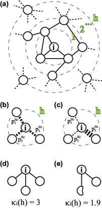
Figure 1: (a) Hierarchical (or concentric) organization around the source node (node $i$). (b) Homogeneous case, where all neighbors are reached with the same probability. (c) Heterogeneous case, where one node has higher probability to be reached. Accessibilities for the (d) homogeneous and (e) heterogeneous case.

In Figure 1(a), we show the hierarchical levels around the source node $i$ up to the distance $h$. The network topology, as well as a type of random walk adopted, will define the transition probabilities, i.e. the components of the vector $\mathbf{p}$. In 1(b) and 1(c) we represent these probabilities by using different widths for the edges. Observe that in both cases, the source node is able to reach $N_{i}(h)=3$ nodes. In the first case, all nodes have the same probability, while in the second case one of the nodes has higher probability than the others. It means that, in the first case, the source node accesses its neighbors in a more uniform manner, which yields an accessibility value equal to 3, as showed in Figure 1(d). On the other hand, the interaction between the source and its neighbors in the second case is biased to a given node, which decreases the effective hierarchical degree to almost 1.9, as showed in Figure 1(e).

It is important to note that the idea of measuring the heterogeneity among first-neighbors nodes in weighted networks was previously proposed in  [25, 26], with the so-called disparity. More recently, in  [27] the authors showed a generalization of this measure, namely the Rényi disparity, which is based on the Rényi entropy. In a particular case, the Rényi disparity uses the Shannon entropy in order to quantify the heterogeneity of weights attached to the edges of a node . This particular case has a similar equation to 1. However, in our case, we consider not only the first-neighbors, but all nodes that can be reached at distance $h$ by a specific dynamic. In this sense, our approach can be also applied to non-weighted networks, since we consider the transition probabilities instead of the edge weights.

Another way to think about the interaction between a source node and its neighbors is by considering the coupon collector problem. This problem  [16, 17] deals with the following question: in the average, how many walks with length $h$ departing from $i$ are required in order to visit all neighboring nodes of $i$ after $h$ steps at least one time? We will call this quantity exploration time of the node $i$ and denote it by $\tau_{i}(h)$, since we can consider the displacement velocity through the network constant. Then, the number of walks is proportional to the time needed to visit all $N_{i}(h)$ nodes. This problem can be mapped into a Poisson problem  [28] with independent variables, which yields the expression 2.

$$\tau_{i}(h)=\int_{0}^{\infty}\left(1-\prod_{j=1}^{N_{i}(h)}\left(1-e^{-xp_{j}^{(h)}}\right)\right)dx$$ (2)

A conjecture has been proposed  [17, 29] that $\tau_{i}$ reaches its minimum value for the homogeneous case, where all neighboring nodes are reached with the same probability, i.e. $p_{j}^{(h)}=1/N_{i}(h)$ for any $j$. In this case, it is not difficult to show that Equation 2 can be rewritten as:

$$\tau_{i}^{hom}(h)=N_{i}(h)\sum_{m=1}^{N_{i}(h)}\frac{1}{m}.$$ (3)

Therefore, by using the conjecture cited above, we can say that the accessibility is maximum whenever the exploration time is minimum. This characteristic is illustrated in Figure  2, which shows a scatter-plot between the accessibility, $\kappa$, and the exploration time, $\tau(h)$, for $10^{5}$ randomly generated vectors $\bf{p}$ with length $N=6$. In this plot it is also shown a set of important curves, which provides a more comprehensive characterization of the probabilities configuration. They correspond to the specific cases where exactly $n$ probabilities have a value $\epsilon$, while all the others $(N-n)$ probabilities are also identical between themselves (so that the sum of all these probabilities becomes equal to one). Therefore, the straight line is related to the case where $n=1$, so that $N-1$ probabilities have the same value. Also, this line corresponds to the bounding value of the accessibility as a function of $\tau(h)$, meaning that all the possible configurations of $\bf{p}$ are enclosed by this curve. The dashed line corresponds to the configurations where $n=2$. Similarly, the dotted line corresponds to the situations where $n=3$, in this case, half of each of the probabilities are equal between themselves. One can use the parametrization $\epsilon$ in Equations 1 and 2 in order to obtain a general equation (indexed C) characterizing these curves:

$$\tau_{C}(\epsilon)=\frac{1}{\epsilon}\sum_{m=1}^{n}\frac{1}{m}+\frac{1}{p}\sum_{m=1}^{N-n}\frac{1}{m}-\\ -\sum_{m=1}^{d}\sum_{m^{\prime}=1}^{N-n}(-1)^{m+m^{\prime}}{n\choose m}{{N-n}\choose{m^{\prime}}}\frac{1}{m\epsilon+m^{\prime}p}$$ (4)

and

$$\kappa_{C}(\epsilon)=\frac{1}{p}\left(\frac{p}{\epsilon}\right)^{\epsilon n},$$ (5)

where $p=(1-n\epsilon)/(N-n)$. Observe that $\epsilon$ lies in the interval $[0,1/n]$. When $\epsilon<1/N$, the upper part of the curves is obtained. In this case, we have $\kappa_{C}\rightarrow N-n$ and $\tau_{C}\rightarrow\infty$ for $\epsilon\rightarrow 0$. For $\epsilon>1/N$, we have the bottom part of the curves, for which $\kappa_{C}\rightarrow n$ and $\tau_{C}\rightarrow\infty$, when $\epsilon\rightarrow 1/n$. When $\epsilon=1/N$, we reach the homogeneous case, where the accessibility is maximum and the exploration time is minimum.

Figure 2: Scatter-plot between the accessibility and the exploration time for $10^{5}$ random vectors with length $N=6$. The lines correspond to the cases where the probabilities are divided in two groups having the same values among themselves as described by Equations 4 and 5 with parametrization $\epsilon$.

III.1 Probabilities in Uniformly Random Networks

Now we investigate the coupon collector problem in uniformly random networks. More specifically, we used 5000 realizations of the Erdős-Rényi model with 200 nodes and average degree 4, and then derived the transition probabilities from these respective networks. We adopted random walks originating from each of the nodes in the networks so as to obtain the respective transition probabilities (the set of $\bf{p}$’s) by using the powers of the transition matrix [30].

Figure 3 presents the distribution of the cases in the $\kappa\times\tau$ space. This result takes into account all cases where the number of accessible nodes, $N_{i}(h)$, is equal to 10 for values of $h$ in the interval $[2,15]$. The gray levels correspond to the density of cases. Remarkably, the density is highly skewed towards the lower bound of the $\epsilon$ curve, and virtually no cases are obtained for the upper half of the probabilities region. This means that it is extremely unlikely to obtain probability configurations having the majority of nodes with higher probability, as illustrated in Figure 2.

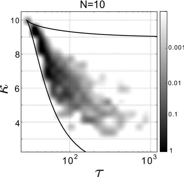
Figure 3: Distribution of the probability configurations in the $\kappa\times\tau$ space obtained for 5000 Erdős-Rényi networks. We considered the cases where 10 nodes are accessible after $h$ steps ($2\leq h\leq 15$) along random walks originating from each of the nodes of the networks.

However, it is possible to obtain configurations which occupy the upper boundary region in the $\kappa\times\tau$ space, where the minority of the probabilities have smaller values. Figure 4(a) presents a particular situation exemplifying this case considering an artificial network with $N$ nodes consisted by two groups: i) a highly connected ER component with $(N-n)$ nodes and average degree $\left<k\right>_{c}$; and ii) $n$ loosely connected nodes with $n_{c}$ ($n_{c}\ll\left<k\right>_{c}$) links to the previous subgraph. This topological division implies that the nodes in the ER component will be much more accessed than the others when considering random walks in this network, irrespective of the starting node and the length $h$. Thus, in the case of $n\ll N$, the probability vectors, $\mathbf{p}^{\prime}s$, will have the majority of their components with higher values, thus occupying the upper region of the $\kappa\times\tau$ space. This property is verified for the simulations presented in Figure 4(b) through randomwalks departing from each node for values of $h$ (varied from 2 to 15) where all nodes are reachable. We considered a single realization of the network with $N=100$ and ER component with $\left<k\right>_{c}$ equal to 50. It was assumed $n=2$ (empty symbols) and $n=20$ (filled symbols) with $n_{c}$ links, varying from 1 to 30, as indicated in the figure. Observe that, as the value of $n_{c}$ decreases, the $n$ nodes become less accessible and the points move away from the origin (the homogeneous case), as expected. Although we assumed that the single nodes are directly connected to the ER component, this example can be immediately extended considering the presence of tails of nodes with different sizes. While this network can be artificially created, obtaining similar results for the occupation of the $\kappa\times\tau$ space, it has been showed [31] that tails are unlikely to occur in great variety of real networks, even for tails with short size. Results for real networks will be shown in the next section.

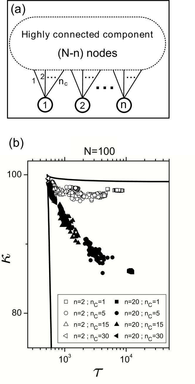
Figure 4: (a) Example of a possible configuration where the upper region of the $\kappa\times\tau$ space is occupied. (b) Results obtained for random walks in the considered network for $n=2$ (empty symbols) and $n=20$ (filled symbols) and different number of connections $n_{c}$.

Figure 5 complements the characterization of the $\kappa\times\tau$ space. It shows: (a) the local average number of steps necessary to reach 10 nodes after departing from the source node; (b) the degree of the source node; and (c) its eigenvector centrality obtained for the probability configurations. It is clear from Figure 5(a) that random walks with larger number of steps (i.e. $h$) tend to have smaller accessibility and longer exploration time. On the other hand, random walks starting from nodes with larger degree (Figure 5(b)) tend to have larger accessibility and shorter exploration times, though in a less definite fashion than that observed in Figure 5(a). Furthermore, Figure 5(c) shows a remarkable centrality pattern: it tends to increase with $\kappa$ while decreasing with $\tau$, apparently following the level set curves in Figure 2. It should be observed that these results are specific for the uniformly random ER networks, in the sense that different trends may be obtained for other theoretical network models.

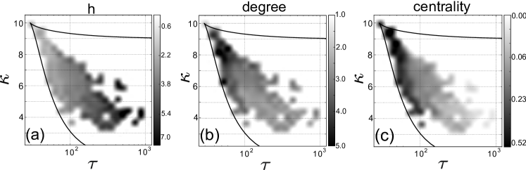
Figure 5: Local average measurements for the probability configurations obtained for 5000 Erdős-Rényi networks. (a) number of steps necessary to reach 10 nodes after departing from the source node, (b) the degree of the source node, and (c) the eigenvector centrality of the source node.

III.2 Real-World Probabilities

We also considered probabilities obtained from real-world networks, namely circuits [32], power grids [33], German highways [34], protein interactions [35], e-mails [36], and co-authorships in network science [37]. The probability configurations obtained from these networks are shown in Figure 6. Again, most of the cases tend to appear near the lower boundary in the $\kappa\times\tau$ space, which is characterized by low exploration time and varying accessibility. This is particularly surprising, as it suggests a universal asymmetry in real networks in which a few probabilities are larger than the others in most configurations. Therefore, it is interesting to observe that real networks, as with the uniformly random topologies, tend to minimize the exploration time at the expense of varying accessibilities.

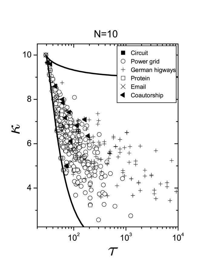
Figure 6: Scatter-plot between the accessibility and the exploration time for 6 real networks considering the cases where $N=10$ nodes are reached after $h=\{2,3,\ldots,20\}$.

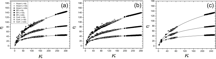
Figure 7: Fraction of reached nodes $\eta_{i}(t,h)$ as a function of the node accessibility $\kappa_{i}$ for (a) classical random walk, (b) self-avoid random walk and (c) preferential random walk. The results are illustrated for the US airlines network and two random counterparts: Erdős-Rényi model and the respective Configuration model [38]. All of them have the same number of nodes ($N=332$) and the same average degree ($\langle k\rangle=12.81$).

Now, we proceed to a related problem in which we are interested to know how many nodes, in the average, are visited during the time interval $t$, while performing a specific type of random walk. This quantity will be denoted by $\eta_{i}(t,h))$ and it provides information about how the network topology around the source node affects the interaction with its neighbors. After a long time, we expect that the source node will be able to visit all $N_{i}(h)$ neighbors, i.e. $\lim_{t\rightarrow\infty}\eta_{i}(t,h))\rightarrow N_{i}(h)$, independent of the vector ${\bf p}_{i}^{(h)}$. Therefore, we can consider that the value of $\eta_{i}(t,h)$ provides an estimate of the average number of visited nodes during a finite time. This is confirmed in Figure  7 for the US airlines network [39] and two random counterparts: Erdős-Rényi model and Configuration model [38]. In order to obtain the transition probabilities, we considered three different types of random walks: (i) traditional random walk (TRW), (ii) preferential random walk (PRW) and (iii) self-avoid random walk (SARW). They were estimated for $h=\ell$, where $\ell=3$ is the network diameter. The TRW and PRW dynamics were calculated by using powers of the transition matrix, while the SARW was estimated through agent-based simulation. This calculation was repeated $10^{6}$ times for each source node. It should be noted that, in the case of SARW dynamics, if an agent cannot proceed further, it remains at the final node contributing to the probabilities for the next steps  [18]. Then, the transition probabilities were used in the equation  1 to evaluate the accessibility of the node $i$. The values of $\eta_{i}(t,h)$ were obtained for each node $i$ as follows: first we draw $t$ neighbors of node $i$ at distance $h=\ell$ according to the obtained probabilities $p_{j}(\ell)$. Then we count how many different nodes were drawn. The average over several realizations gives us an estimate of $\eta_{i}(t,h)$. The behavior of $\kappa$ versus $\eta$ is showed in Figure 7a, 7b and 7c for TRW, SARW and PRW respectively. The results have been found to be well-fitted by the functional form represented in Equation 6.

$$\eta=a+b\log(\kappa+c)$$ (6)

It is interesting to observe in Figure 7c that when the preferential rules were adopted, the fraction of reached nodes was strongly decreased in the US airline and its configuration model. This is a direct consequence of the degree heterogeneity of these networks. For preferential random walk, the walks are biased to pass through nodes with high connectivity, so that several possible paths are not used. Therefore, the effective number of reached nodes is smaller than in the cases where we considered self-avoid or traditional random walk. As we can see, this phenomena is not observed in ER networks, which have a more homogeneous degree distribution.

IV Conclusions

The accessibility concept was introduced recently [18] as a means to quantify the potential of a node to interact with other nodes in a complex network. Given the many promising results obtained so far, it became important to better understand the accessibility concept, specially regarding optimization aspects. The present work focused on the investigation of the accessibility regarding the coupon collector problem as well as its relationship with the average number of nodes visited along a random walk during a given time interval.

A number of remarkable results were obtained about the relationship between the accessibility and the exploration time. First, we have that the minimal exploration time is obtained for the maximum accessibility. No relationship between these two properties have been observed otherwise, i.e. when we consider all possible probabilities configurations. However, in the cases of uniformly random and real-world networks, a stronger correlation is verified, with the cases tending to lie near the lower boundary in the $\kappa\times\tau$ space. As a matter of fact, there is a very low probability of having cases occupying the upper half portion of this space. Although this could suggest some intrinsic impossibility of having such cases, we showed at least one type of topology leading to a configuration lying over the upper boundary. This remarkable result shows that in all considered networks the transition probability configurations tend to be characterized by small exploration time at the expense of varying accessibilities.

Regarding the relationship between the accessibility and the average number of nodes visited along a random walk during a given time interval, we showed that the concept of accessibility can be understood as a generalization of the classical degree, in the sense that the accessibility quantifies the effective number of nodes that can be reached from the source node after a given number of steps. In order to confirm this statement, we also showed that there is a strong relationship between the accessibility and the inverse coupon collector problem, which deals with the number of visited nodes in a finite time interval.

Future works could take into a account activations originating from multiple nodes as well as how other dynamical properties can be predicted from the accessibility values. It would be particularly interesting to identify more general theoretical models and real networks capable of covering the $\kappa\times\tau$ more uniformly.

- [1] S. N. Dorogovtsev and A. V. Goltsev. Critical phenomena in complex networks. Rev. Mod. Phys., 80(4):1275–1335, 2008.
- [2] A. Barrat, M. Barth lemy, and A. Vespignani. Dynamical Processes on Complex Networks. Cambridge University Press, 2008.
- [3] S. Boccaletti, V. Latora, Y. Moreno, M. Chavez, and D. U. Hwang. Complex networks: structure and dynamics. Physics Reports, 424(4-5):175–308, 2006.
- [4] L. K. Gallos and P. Argyrakis. Absence of kinetic effects in reaction-diffusion processes in scale-free networks. Phys. Rev. Lett., 92(13):138301, 2004.
- [5] R. Olfati-Saber, J. A. Fax, and R. M. Murray. Consensus and cooperation in networked multi-agent systems. Proceedings of the IEEE, 95(1):215–233, 2007.
- [6] P. Holme. Congestion and centrality in traffic flow on complex networks. Advances in Complex Systems, 6(2):163–176, 2003.
- [7] B. Tadic, G.J. Rodgers, and S. Thurner. Transport on complex networks: Flow, jamming and optimization. Int. J. Bifurcation and Chaos, 17(7):2363–2385, 2007.
- [8] R. Guimera, A. Arenas, A. Diaz-Guilera, and F. Giralt. Dynamical properties of model communication networks. Phys. Rev. E, 66(2), 2002.
- [9] B. Kozma B, M. B. Hastings, and G. Korniss. Diffusion processes on power-law small-world networks. Phys. Rev. Lett, 95(1):018701, 2005.
- [10] Z. Dezso, E. Almaas, A. Lukacs, B. Racz, I. Szakadat, and A. L. Barabasi. Dynamics of information access on the web. Phys. Rev. E, 73(6), 2006.
- [11] M. Kitsak, L. K. Gallos, S. Havlin, F. Liljeros, L. Muchnik, H. E. Stanley, and H. A. Makse. Identification of influential spreaders in complex networks. Nature Physics, 6(11):888–893, 2010.
- [12] J. O. H. Bakke, A. Hansen, and J. Kertesz. Failures and avalanches in complex networks. Europhys. Lett., 76(4):717–723, 2006.
- [13] P. R. V. Boas, F. A. Rodrigues, and L. da F. Costa. Modeling worldwide highway networks. Physics Letters A, 374(1):22–27, 2009.
- [14] D. O. Cajueiro. Optimal navigation for characterizing the role of the nodes in complex networks. Physica A: Statistical Mechanics and its Applications, 389(9):1945–1954, 2010.
- [15] S. E. Ahnert, B. A. N. Travençolo, and L. da F. Costa. Connectivity and dynamics of neuronal networks as defined by the shape of individual neurons. New J. Phys., 11:103053, 2009.
- [16] P. Frajolet, D. Gardi, and L. Thimonier. Birthday paradox, coupon collectors, caching algorithms and self-organizing search. Discrete Applied Mathematics, 39:207–229, 1992.
- [17] A. Boneh and M Hofri. The coupon-collector problem revisited - a survey of engineering problems and computational methods. Stochastic Models, 13(1):39–66, 1997.
- [18] B. A. N. Traven olo and L. da F. Costa. Accessibility in complex networks. Phys. Lett. A, 373(1):89–95, 2008.
- [19] F. N. Silva and L. da F. Costa. Hierarchical characterization of complex networks. Journal of Statistical Physics, 125(4):841–872, 2006.
- [20] B. A. N. Traven olo, M. P. Viana, and L. da F. Costa. Border detection in complex networks. New J. Phys., 11:063019, 2010.
- [21] L. Antiqueira and L. da F. Costa. Structure-dynamics interplay in directed complex networks with border effects. in: Complenet 2010. Proceedings of the 2nd Workshop on Complex Networks., 2010.
- [22] M. P. Viana, B. A. N. Traven olo, E. Tanck, and L. da F. Costa. Characterizing topological and dynamical properties of complex networks without border effects. Physica A: Statistical Mechanics and its Applications, 389(8):1771–1778, 2010.
- [23] F. N. Silva, B. A. N. Traven olo, M. P. Viana, and L. da F. Costa. Identifying the borders of mathematical knowledge. J. Phys. A: Math. Theor, 43(32), 2010.
- [24] L. da F. Costa, B. A. N. Traven olo, M. P. Viana, and E. Strano. On the efficiency of transportation systems in large cities. Europhys. Lett., 91(1), 2010.
- [25] E. Almaas, B. Kov cs, T. Vicsek, Z. N. Oltvai, and A.-L. Barab si. Global organization of metabolic fluxes in the bacterium escherichia coli. Nature, 427:839–843, 2004.
- [26] M. Barth lemya, A. Barratb, R. Pastor-Satorras, and A. Vespignani. Characterization and modeling of weighted networks. Physica A: Statistical Mechanics and its Applications, 346(1-2):34–43, 2005.
- [27] S. H. Lee, P. J. Kim, Y. Y. Ahn, and H. Jeong. Googling social interactions: Web search engine based social network construction. PLOS ONE, 5(7):e11233, 2010.
- [28] P. Berenbrink and T. Sauerwald. The weighted coupon collector’s problem and applications. In Proceedings of the 15th Annual International Conference on Computing and Combinatorics, COCOON ’09, pages 449–458. Springer-Verlag, 2009.
- [29] R. J. Caron, M. Hlynka, and J. F. McDonald. On the best-case performance of probabilistic methods for detecting necessary constraints. Technical Report WMSR-88-02, 1988.
- [30] J. D. Noh and H. Rieger. Random walks on complex networks. Phys. Rev. Letts., 92:118701, 2004.
- [31] P. R. Villas-Boas, F. A. Rodrigues, G. Travieso, and L. da F. Costa. Chain motifs: The tails and handles of complex networks. Phys. Rev. E, 77(2):026106, 2008.
- [32] R. Milo, S. Itzkovitz, N. Kashtan, R. Levitt, S. Shen-Orr, I. Ayzenshtat, M. Sheffer, and U. Alon. Superfamilies of evolved and designed networks. Science, 303:1538–1542, 2004.
- [33] D. J. Watts and S. H. Strogatz. Collective dynamics of ’small-world’ networks. Nature, 393:440–442, 1998.
- [34] M. Kaiser and C. C. Hilgetag. Spatial growth of real-world networks. Phys. Rev. E, 69:036103, 2004.
- [35] G. Palla, I. Der nyi, I. Farkas, and T. Vicsek. Uncovering the overlapping community structure of complex networks in nature and society. Nature, 435:814–818, 2005.
- [36] R. Guimera, L. Danon, A. Diaz-Guilera, F. Giralt, and A. Arenas. Self-similar community structure in a network of human interactions. Phys. Rev. E, 68:065103, 2003.
- [37] M. E. J. Newman. Finding community structure in networks using the eigenvectors of matrices. Phys. Rev. E, 74:036104, 2006.
- [38] M. Molloy and B. Reed. A critical point for random graphs with a given degree sequence. Random Struct. Algorithms, 6:161–179, 1995.
- [39] B. Vladimir and M. Andrej. Pajek datasets., 2006.