Beam-beam simulation code BBSIM for particle accelerators

Abstract

A highly efficient, fully parallelized, six-dimensional tracking model for simulating interactions of colliding hadron beams in high energy ring colliders and simulating schemes for mitigating their effects is described. The model uses the weak-strong approximation for calculating the head-on interactions when the test beam has lower intensity than the other beam, a look-up table for the efficient calculation of long-range beam-beam forces, and a self-consistent Poisson solver when both beams have comparable intensities. A performance test of the model in a parallel environment is presented. The code is used to calculate beam emittance and beam loss in the Tevatron at Fermilab and compared with measurements. We also present results from the studies of two schemes proposed to compensate the beam-beam interactions: a) the compensation of long-range interactions in the Relativistic Heavy Ion Collider (RHIC) at Brookhaven and the Large Hadron Collider (LHC) at CERN with a current-carrying wire, b) the use of a low-energy electron beam to compensate the head-on interactions in RHIC.

1 Introduction

In high energy storage-ring colliders, the beam-beam interactions are known to cause emittance growth and a reduction of beam life time, and to limit the collider luminosity [1, 2, 3, 4, 5, 6, 7]. It has been a key issue in a high energy collider to simulate the beam-beam interaction accurately and to mitigate the interaction effects. A beam-beam simulation code BBSIM has been developed at Fermilab over the past few years to study the effects of the machine nonlinearities and the beam-beam interactions [8, 9, 10, 11]. The code is under continuous development with the emphasis being on including the important details of an accelerator and the ability to reproduce observations in diagnostic devices. At present, the code can be used to calculate tune footprints, dynamic apertures, beam transfer functions, frequency diffusion maps, action diffusion coefficients, emittance growth, and beam lifetime. Calculation of the last two quantities over the long time scales of interest is time consuming even with modern computer technology. In order to run efficiently on a multiprocessor system, the resulting model was implemented by using parallel libraries which are MPI (inter-processor Message Passing Interface standard) [12], state-of-the-art parallel solver libraries (Portable, Extensible Toolkit for Scientific Calculation, PETSc) [13], and HDF5 (Hierarchical Data Format) [14].

The organization of the paper is as follows: The physical model used in the simulation code is described in Section 2. The parallelization algorithm and performance are described in Section 3. Some applications are presented for the Tevatron, the Relativistic Heavy Ion Collider (RHIC) and the Large Hadron Collider (LHC) in Section 4. Section 5 summarizes our results.

2 Physical model

In a collider simulation, the two beams moving in opposite direction are represented by macroparticles. The macroparticles are generated with the same charge to mass ratio as the particles in the accelerator. The number of macroparticles chosen is much less than the bunch intensity of the beam because it becomes prohibitive to follow approximately 10¹¹ particles for even a few revolutions around the accelerator using modern supercomputers. These macroparticles are generated and loaded with an initial distribution chosen for the specific simulation purpose. As an example, a six-dimensional Gaussian distribution is used for long-term beam evolution. The transverse and longitudinal motion of particles is calculated by a sequence of linear and nonlinear transfer maps. During the beam transport, a particle is removed from the distribution if it reaches a predefined boundary in transverse or longitudinal direction. In our simulation model, the following effects are included: head-on and long-range beam-beam interactions, fields of a current-carrying wire and an electron lens, multipole errors in quadrupole magnets in interaction regions, sextupoles for chromaticity correction, ac dipole, resistive wall wake, tune modulation, noise in lattice elements, single and multiple harmonic rf cavities, and crab cavities. The finite bunch length effect of the beam-beam interactions is considered by slicing the beam into several chunks in the longitudinal direction and then applying a synchro-beam map [15]. Each slice in a beam interacts with slices in the other beam in turn at a collision point. In the following, linear and nonlinear tracking models are described in detail.

2.1 Transport through an arc

The six-dimensional coordinates of a test particle in the accelerator’s coordinate frame are: $\mathbf{x}=\left(x,x^{{}^{\prime}},y,y^{{}^{\prime}},z,\delta\right)^{T}$, where $x$ and $y$ are horizontal and vertical coordinates, $x^{\prime}$ and $y^{\prime}$ the trajectory slopes of the coordinates, $z=-c\Delta t$ the longitudinal distance from the synchronous particle, and $\delta=\Delta p_{z}/p_{0}$ the relative momentum deviation from the synchronous energy [16]. The transverse linear transformation between two elements denoted by $i$ and $j$ can be written as

$$\mathbf{x}_{j}=\left(\begin{array}[]{cc}\mathcal{M}&\hat{\mathcal{D}}\\ \hat{\mathcal{A}}&\mathcal{L}\end{array}\right)\mathbf{x}_{i}.$$ (1)

Here, $\mathcal{M}$ is a coupled transverse map of off-momentum motion defined by $\mathcal{M}=\mathcal{R}_{j}\tilde{\mathcal{M}}_{i\rightarrow j}\mathcal{R}_{i}^{-1}$, where $\tilde{\mathcal{M}}_{i\rightarrow j}$ is the uncoupled linear map described by Twiss functions at $i$ and $j$ elements, and the transverse coupling matrix $\mathcal{R}$ is defined as [17]

$$\mathcal{R}=\frac{1}{\sqrt{1+\left|C\right|}}\left(\begin{array}[]{cc}I&C^{\dagger}\\ -C&I\end{array}\right)$$ (2)

where $C^{\dagger}$ is the $2\times 2$ matrix and the symplectic conjugate of the coupling matrix $C$. The $4\times 2$ dispersion matrix is defined by $\hat{\mathcal{D}}=\left(0,\mathbf{D}\right)$, and the dispersion vector $\mathbf{D}=\left(D_{x},D_{x}^{{}^{\prime}},D_{y},D_{y}^{{}^{\prime}}\right)^{T}$ is characterized by the transverse dispersion functions and the map $\mathcal{M}$, i.e., $\mathbf{D}=\mathbf{D}_{j}-\mathcal{M}\mathbf{D}_{i}$ where $\mathbf{D}_{i},\mathbf{D}_{j}$ are the dispersion vectors at $i,j$. Since the transport matrix has to be symplectic, the matrix $\hat{\mathcal{A}}$ in Eq. (1) is given by $\hat{A}=-\hat{\mathcal{D}}^{T}S^{T}\mathcal{M},$ where $S$ is a rearranging matrix (see subsection 2.7). The longitudinal map $\mathcal{L}$ is given by $\mathcal{L}=\left(\begin{array}[]{cc}1&-\left(\eta/\beta\right)\Delta s\\ 0&1\end{array}\right)$, where $\eta$ is the slip factor, $\beta=v/c$, and $\Delta s$ the longitudinal distance between the two elements, i.e., $\Delta s=s_{j}-s_{i}$. It is noted that $s$ is the axis along the beam direction. The nonlinearity of synchrotron oscillations is applied by adding the longitudinal momentum change at a rf cavity:

$$\Delta\delta=\frac{eV_{rf}}{\beta^{2}E}\left(\sin k_{rf}z-\sin\phi_{s}\right)$$ (3)

where $V_{rf}$ is the voltage of rf cavity, $\phi_{s}$ the phase angle for a synchronous particle with respect to the rf wave, and $k_{rf}$ the wave number of the rf cavity. If there are higher harmonic cavities, their effects are added to the momentum change.

2.2 Beam-beam interactions

In order to achieve high luminosity in a collider one can increase the number of bunches which reduces the bunch spacing. More bunches can increase the number of parasitic encounters in the interaction regions. Since the calculation of beam-beam forces requires large amounts of computational resources, it has to be executed rapidly and accurately. BBSIM has three different models for this purpose: a weak-strong model for head-on interactions, a look-up table model for long-range interactions, and a Poisson solver model for the head-on interactions when both beams have comparable intensities (“strong-strong” model).

2.2.1 Weak-strong model

In the weak-strong model we assume that the “weak” beam is affected by the head-on and long-range interactions while the opposing beam or “strong” beam is unaffected. The charge distribution of the strong beam is assumed to be Gaussian:

$$\rho\left(x,y,z\right)=\frac{Nq}{\left(2\pi\right)^{3/2}\sigma_{x}\sigma_{y}\sigma_{z}}\exp\left(-\frac{x^{2}}{2\sigma_{x}^{2}}-\frac{y^{2}}{2\sigma_{y}^{2}}-\frac{z^{2}}{2\sigma_{z}^{2}}\right)$$ (4)

Here, $N$ is the number of particles per bunch and $q$ is the charge per particle. Note that the coordinates $\left(x,y,z\right)$ are measured in the rest frame of the strong beam. The beam-beam force between two beams with transverse Gaussian distribution $\rho\left(x,y\right)=\int dz\rho\left(x,y,z\right)$ is well-known [18], and the expression for the slope change is given by, for elliptical beam with $\sigma_{x}>\sigma_{y}$:

$$\left(\begin{array}[]{c}\Delta x^{\prime}\\ \Delta y^{\prime}\end{array}\right)=\frac{2Nr_{0}}{\gamma}\frac{\sqrt{\pi}}{\sqrt{2\left(\sigma_{x}^{2}-\sigma_{y}^{2}\right)}}\left(\begin{array}[]{c}\text{Im}\left[F\left(x,y\right)\right]\\ \text{Re}\left[F\left(x,y\right)\right]\end{array}\right)$$ (5)

where

$$F\left(x,y\right)=w\left(\frac{x+iy}{\sqrt{2\left(\sigma_{x}^{2}-\sigma_{y}^{2}\right)}}\right)-e^{-\frac{x^{2}}{2\sigma_{x}^{2}}-\frac{y^{2}}{2\sigma_{y}^{2}}}w\left(\frac{\frac{x\sigma_{y}}{\sigma_{x}}+i\frac{y\sigma_{x}}{\sigma_{y}}}{\sqrt{2\left(\sigma_{x}^{2}-\sigma_{y}^{2}\right)}}\right).$$ (6)

Here, $w\left(z\right)$ is the complex error function defined by $w\left(z\right)=e^{-z^{2}}\left(1+\frac{2i}{\sqrt{\pi}}\int_{0}^{z}dt\,e^{t^{2}}\right)$, and $\gamma$ the Lorentz factor. The constant $r_{0}$ is defined as $r_{0}\equiv qq_{*}/4\pi\epsilon_{0}m_{0}c^{2}$, where $q_{*}$ is the electric charge of the test particle, and $m_{0}$ the rest mass of the particle.

2.2.2 Look-up table model

The charge distribution of the strong beam in the weak-strong model is not varied during the simulations. It is redundant to re-calculate the beam-beam force at every parasitic location and every turn. A look-up table is one way to avoid it. The look-up table is used to replace a run time computation with an array indexing operation. The beam-beam force of a Gaussian beam distribution is described by the complex error function, as shown in Eq. (6). The calculation of the complex error function can substantially slow the beam-beam simulation. However, the look-up table is pre-calculated and stored in a memory, usually in an array. When the value of the error function is required, it can be retrieved from the table by an interpolation scheme, instead of using Eq. (6). The look-up table method can significantly reduce a computational cost. The property of the complex error functions yields the symmetry relations of function $F\left(z\right)$ as

$$F\left(-z\right)=-F\left(z\right),\;F\left(\bar{z}\right)=-\overline{F\left(z\right)},\;F\left(-\bar{z}\right)=\overline{F\left(z\right)}$$ (7)

where $z=x+iy$ is a complex variable. The symmetry conditions of the function $F\left(z\right)$ can reduce memory space to store the function values. It is sufficient to build the table for the values of function $F\left(z\right)$ in the first quadrant of the complex plane, i.e., $\left|x\right|\geq 0$ and $\left|y\right|\geq 0$.

Interpolation techniques are required to predict a value of a function at a point inside its domain based upon the known tabulated values. For a given set of data points $\left(z_{i},f_{i}\right)$, $i=0,\dots,N$, where no two $z_{i}$’s are the same, the interpolated value $g\left(z\right)$ at a value $z\neq z_{i}$ is found from

$$g\left(z\right)=\sum_{i=0}^{N}f_{i}L_{i}\left(z\right)$$ (8)

where the $L_{i}$ is Lagrange’s $N$-th order polynomials

$$L_{i}\left(z\right)=\prod_{j=0,j\neq i}^{N}\frac{z-z_{j}}{z_{i}-z_{j}}.$$ (9)

In order to save the interpolation time further, one can divide $z$-space and apply a different degree of the Lagrange polynomial. For an example, we apply a sixth order polynomial for small amplitudes $\left|z\right|\leq 4\sigma$ while a third order polynomial is applied for $\left|z\right|>4\sigma$, because the function $F\left(z\right)$ varies more rapidly at small $\left|z\right|$ and slowly at large $\left|z\right|$ .

2.2.3 Poisson solver model

The weak-strong model is a good approximation when one beam has much smaller intensity than the other, but it is not valid when the intensities of the two beams are comparable because each beam’s parameters are changed by the other beam. One has to solve for the field of each beam self-consistently. The fields are the solutions of the Poisson equation given by

$$\nabla^{2}\phi\left(\mathbf{r}\right)=-4\pi\rho\left(\mathbf{r}\right)$$ (10)

where $\phi$ is the electrostatic potential and $\rho$ the density function of the beam. The solution can be obtained by

$$\phi\left(\mathbf{r}\right)=\int G\left(\mathbf{r},\mathbf{r}_{1}\right)\rho\left(\mathbf{r}_{1}\right)d\mathbf{r}_{1}$$ (11)

where $G$ is the Green’s function of the Poisson equation and in two space dimension, is given by

$$G\left(x,y:x_{1},y_{1}\right)=-\frac{1}{4\pi}\ln\left[\left(x-x_{1}\right)^{2}+\left(y-y_{1}\right)^{2}\right].$$ (12)

Equation (11) can be efficiently calculated using a convolution theorem and inverse Fourier transform:

$$\phi\left(\mathbf{r}\right)=\mathcal{F}^{-1}\left(\hat{G}\left(\bm{\omega}\right)\hat{\rho}\left(\bm{\omega}\right)\right)$$ (13)

where $\hat{G}\left(\bm{\omega}\right)=\left(\frac{1}{\sqrt{2\pi}}\right)^{2}\int_{\mathbb{R}^{2}}G\left(\mathbf{r}\right)e^{-i\bm{\omega}\cdot\mathbf{r}}d\mathbf{r}$ and $\hat{\rho}\left(\bm{\omega}\right)=\left(\frac{1}{\sqrt{2\pi}}\right)^{2}\int_{\mathbb{R}^{2}}\rho\left(\mathbf{r}\right)e^{-i\bm{\omega}\cdot\mathbf{r}}d\mathbf{r}$. It is assumed in Eq. (13) that the density function $\rho\left(\mathbf{r}\right)$ is periodic in both $x$ and $y$ directions. However, since the beam has a finite charge distribution surrounded by a conducting wall in an accelerator system, the transverse beam density does not meet the periodicity requirement of FFT techniques. In order to apply the above formalism, the density function should be rewritten by, in the doubled computational domain [19]:

$$\rho_{new}\left(x,y\right)=\begin{cases}\rho\left(x,y\right)&,\;0<x\leq L_{x},\;0<y\leq L_{y}\\ 0&,\;L_{x}<x\leq 2L_{x},\;or\;L_{y}<y\leq 2L_{y}.\end{cases}$$ (14)

Green’s function is defined in the doubled domain, as follows:

$$G_{new}\left(x,y\right)=\begin{cases}G\left(x,y\right)&,\,0<x\leq L_{x},\;0<y\leq L_{y}\\ G\left(2L_{x}-x,y\right)&,\,L_{x}<x\leq 2L_{x},\;0<y\leq L_{y}\\ G\left(x,2L_{y}-y\right)&,\,0<x\leq L_{x},\;L_{y}<y\leq 2L_{y}\\ G\left(2L_{x}-x,2L_{y}-y\right)&,\,L_{x}<x\leq 2L_{x},\;L_{y}<y\leq 2L_{y}.\end{cases}$$ (15)

Both $\rho_{new}$ and $G_{new}$ are doubly periodic functions with periods $2L_{x}$ and $2L_{y}$. It is noted that only the potential within a domain $\left(0,L_{x}\right]\times\left(0,L_{y}\right]$ is valid. The potential outside the domain is incorrect, but it doesn’t matter because the physical domain of interest is $\left(0,L_{x}\right]\times\left(0,L_{y}\right]$. When one beam is separated far from the other, one can apply a shifted Green’s function approach [20].

2.2.4 Crossing angle

When there exists a finite crossing angle between two colliding beams at an interaction point, the beam-beam force experienced by a test particle will have transverse and longitudinal components because the electric field generated by the opposing beam is not perpendicular to the particle velocity anymore. The existence of a longitudinal force makes it difficult to apply the result of previous sections. A transformation can be used to remedy the difficulty. It transforms a crossing angle collision in the laboratory frame to a head-on collision in the rotated and boosted frame which is called the head-on frame [21, 22]. The transformation can be described by a transformation from the accelerator coordinates to Cartesian coordinates, a Lorentz boost, and again a backward transformation to the accelerator coordinates:

$$x^{*} =z\cos\alpha\tan\phi+x\left[1+h_{x}^{*}\cos\alpha\sin\phi\right]+yh_{x}^{*}\sin\alpha\sin\phi$$ (16)

$$y^{*} =z\sin\alpha\tan\phi+y\left[1+h_{y}^{*}\sin\alpha\sin\phi\right]+xh_{y}^{*}\cos\alpha\sin\phi$$

$$z^{*} =\frac{z}{\cos\phi}+h_{z}^{*}\left[x\cos\alpha\sin\phi+y\sin\alpha\sin\phi\right]$$

$$p_{x}^{*} =\frac{p_{x}}{\cos\phi}-h\cos\alpha\frac{\tan\phi}{\cos\phi}$$

$$p_{y}^{*} =\frac{p_{y}}{\cos\phi}-h\sin\alpha\frac{\tan\phi}{\cos\phi}$$

$$p_{z}^{*} =p_{z}-p_{x}\cos\alpha\tan\phi-p_{y}\sin\alpha\tan\phi+h\tan^{2}\phi$$

where a star (*) stands for a dynamical variable in the head-on frame, the Hamiltonian $h\left(p_{x},p_{y},p_{z}\right)=p_{z}+1-\sqrt{\left(p_{z}+1\right)^{2}-p_{x}^{2}-p_{y}^{2}}$, $h_{x}^{*}=\partial h^{*}/\partial p_{x}^{*}$, $h^{*}\left(p_{x}^{*},p_{y}^{*},p_{z}^{*}\right)=h\left(p_{x}^{*},p_{y}^{*},p_{z}^{*}\right)$, $\alpha$ the crossing plane angle in the $x-y$ plane, and $\phi$ the half crossing angle in the $\tilde{x}-s$ plane as shown in Fig. 1.

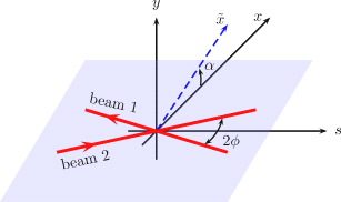
Figure 1: Definition of crossing angles $\alpha$ and $\phi$: $\alpha$ is the crossing plane angle in the $x-y$ plane and $\phi$ is the half crossing angle in the $\tilde{x}-s$ plane. $s$ is the axis along the beam direction when there is no crossing angle. The $\tilde{x}-s$ plane is the crossing plane defined by the angle $\alpha$. The beam trajectories, shown by lines with arrows, lie in the crossing plane.

2.3 Finite bunch length

The effects due to the finite (as opposed to infinitesimal) bunch length need to be considered when the transverse beta functions at the interaction point are small and comparable to $\sigma_{z}$. The finite longitudinal length is considered by dividing the beam into longitudinal slices and by a so called synchro-beam map [15]. We make slices of both beams moving in opposite directions. Each slice of the strong bunch is integrated over its length, and has only a transverse charge distribution at its center. We take into account the collision between a pair of slices: the $i^{th}$ slice of a bunch and the $j^{th}$ slice of a bunch in the other beam. The collision takes place at collision point $S\left(z^{i},z_{*}^{j}\right)=\frac{1}{2}\left(z^{i}-z_{*}^{j}\right)$ which is usually different from the interaction point. For example, the $i^{th}$ slice of a bunch has successive collisions with slices of a bunch in the other beam. In addition, the electric field varies along the bunch due to the inhomogeneity of the charge density in the longitudinal direction, and couples transverse and longitudinal motions. The coupling can be modeled by the synchro-beam map which includes beam-beam interactions due to the longitudinal component of the electric field as well as the transverse components. The transformation is given by [15]

$$x^{new} =x+S\left(z,z_{*}\right)\left.\frac{\partial U}{\partial x}\right|_{S},\enskip p_{x}^{new}=p_{x}-\left.\frac{\partial U}{\partial x}\right|_{S}$$ (17)

$$y^{new} =y+S\left(z,z_{*}\right)\left.\frac{\partial U}{\partial y}\right|_{S},\;p_{y}^{new}=p_{y}-\left.\frac{\partial U}{\partial y}\right|_{S}$$

$$z^{new} =z,\>\delta^{new}=\delta-\frac{1}{2}\left.\frac{\partial U}{\partial x}\right|_{S}\left[p_{x}-\frac{1}{2}\left.\frac{\partial U}{\partial x}\right|_{S}\right]-\frac{1}{2}\left.\frac{\partial U}{\partial y}\right|_{S}\left[p_{y}-\frac{1}{2}\left.\frac{\partial U}{\partial y}\right|_{S}\right]-\frac{1}{2}\left.\frac{\partial U}{\partial z}\right|_{S}.$$

Here, $\left.\right|_{S}$ represents the evaluation at the collision point $S\left(z,z_{*}\right)$. $U$ is the normalized potential energy $U=q\Phi/E_{0}$ and is given by

$$U\left(x,y;\sigma_{x}\left(s\right),\sigma_{y}\left(s\right)\right)=\frac{N_{*}r_{0}}{\gamma}\int_{0}^{\infty}d\zeta\frac{-1+\exp\left(-\frac{x^{2}}{2\sigma_{x}^{2}+\zeta}-\frac{y^{2}}{2\sigma_{y}^{2}+\zeta}\right)}{\sqrt{\left(2\sigma_{x}^{2}+\zeta\right)\left(2\sigma_{y}^{2}+\zeta\right)}}.$$ (18)

The dependence on the bunch length is contained in $\sigma_{x}(s),\sigma_{y}(s)$. The transverse derivatives of the potential energy are

$$\left.\frac{\partial U}{\partial x}\right|_{S}=-\Delta x^{\prime}\left(X,Y;S\left(z,z_{*}\right)\right),\;\left.\frac{\partial U}{\partial y}\right|_{S}=-\Delta y^{\prime}\left(X,Y;S\left(z,z_{*}\right)\right)$$ (19)

where $\left(X,Y\right)$ are the transverse coordinates at $S\left(z,z_{*}\right)$, and$\Delta x^{\prime}$ and $\Delta y^{\prime}$ are given by Eq. (5). The longitudinal derivative of the potential energy which is related to the longitudinal beam-beam kicks is expressed by

$$\left.\frac{\partial U}{\partial z}\right|_{S} =\frac{1}{2}\left.\frac{d\sigma_{x}^{2}}{ds}\frac{\partial U}{\partial\sigma_{x}^{2}}\right|_{s=S\left(z,z_{*}\right)}+\frac{1}{2}\left.\frac{d\sigma_{y}^{2}}{ds}\frac{\partial U}{\partial\sigma_{y}^{2}}\right|_{s=S\left(z,z_{*}\right)}$$ (20)

$$\frac{\partial U}{\partial\sigma_{x}^{2}} =\frac{1}{2\left(\sigma_{x}^{2}-\sigma_{y}^{2}\right)}\left[x\Delta x^{\prime}+y\Delta y^{\prime}+\frac{2N_{*}r_{0}}{\gamma}\left(\frac{\sigma_{y}}{\sigma_{x}}e^{-\frac{x^{2}}{2\sigma_{x}^{2}}-\frac{y^{2}}{2\sigma_{y}^{2}}}-1\right)\right]$$

$$\frac{\partial U}{\partial\sigma_{y}^{2}} =\frac{-1}{2\left(\sigma_{x}^{2}-\sigma_{y}^{2}\right)}\left[x\Delta x^{\prime}+y\Delta y^{\prime}+\frac{2N_{*}r_{0}}{\gamma}\left(\frac{\sigma_{x}}{\sigma_{y}}e^{-\frac{x^{2}}{2\sigma_{x}^{2}}-\frac{y^{2}}{2\sigma_{y}^{2}}}-1\right)\right].$$

Note that $\frac{d\sigma_{x}^{2}}{ds}$ and $\frac{d\sigma_{y}^{2}}{ds}$ have zero amplitude and change their sign at the interaction point if $\alpha_{x}=\alpha_{y}=0$. Test particles experience longitudinal acceleration and deceleration passing through the bunch moving in the opposite direction.

2.4 Compensation schemes

In storage-ring colliders, a beam experiences periodic perturbations when it meets the counter-rotating beam in a common beam pipe. The head-on beam-beam interactions occur when the beams collide in the detectors while the long-range interactions occur when the beams are simultaneously present at the same location but are separated transversely. The nonlinear forces due to these beam-beam interactions result in a tune spread and can cause emittance growth, a reduction of beam life time, and therefore reduce the collider luminosity. The combination of beam-beam and machine nonlinearities excites betatron resonances which can cause particles to diffuse into the tails of the beam distribution and even to the physical aperture. Different compensation methods have been proposed: a current-carrying wire for the effects of the long-range interactions [23] and an electron lens for the head-on interactions in proton machines [24, 25, 26]. Beam collisions with a crossing angle at the interaction point are often necessary in colliders to reduce the effects of the long-range interactions. The crossing angle reduces the geometrical overlap of the beams and hence the luminosity. A deflecting mode cavity, also known as a crab cavity, offers a promising way to compensate the crossing angle and to realize effective head-on collisions [27, 28]. We now describe the modeling of these compensation schemes in the program.

2.4.1 Current-carrying wire

When the separations at long-range interactions are large compared to the rms beam size the strength of these interactions is inversely proportional to the distance. Its effect on a beam can be compensated by a current-carrying wire which creates a magnetic field with the same $\frac{1}{r}$ dependence. This approach is simple and it is possible to deal with all multipole orders at once. For a finite length $l_{w}$ embedded in the middle of a drift length $L$, the transfer map of a wire can be obtained by

$$\mathcal{M}_{w}^{\left(L\right)}=D_{L/2}\circ\mathcal{M}_{k}^{\left(L\right)}\circ D_{L/2}$$ (21)

where $D_{L/2}$ is the drift map with a length $\frac{L}{2}$, and $\mathcal{M}_{k}^{\left(L\right)}$ is the wire kick integrated over a drift length. This kick map $\mathcal{M}_{k}^{\left(L\right)}$ is reproduced by the following changes in slope [29]

$$\left(\begin{array}[]{c}\Delta x^{\prime}\\ \Delta y^{\prime}\end{array}\right)=\frac{\mu_{0}}{4\pi}\frac{I_{w}l_{w}}{\left(B\rho\right)}\frac{u-v}{x^{2}+y^{2}}\left(\begin{array}[]{c}x\\ y\end{array}\right)$$ (22)

where $I_{w}$ is the current of the wire , $u=\sqrt{\left(\frac{L}{2}+l_{w}\right)^{2}+x^{2}+y^{2}}$ and $v=\sqrt{\left(\frac{L}{2}-l_{w}\right)^{2}+x^{2}+y^{2}}$. We also take into account the wire misalignment including pitch and yaw angles $\left(\theta_{x},\theta_{y}\right)$ respectively as well as lateral shifts $\left(\Delta x,\Delta y\right)$. The transfer map of a wire can be written as

$$\mathcal{M}_{w}=S_{\Delta x,\Delta y}\circ T_{\theta_{x},\theta_{y}}^{-1}\circ D_{L/2}\circ\mathcal{M}_{k}^{\left(L\right)}\circ D_{L/2}\circ T_{\theta_{x},\theta_{y}}$$ (23)

where $T_{\theta_{x},\theta_{y}}$ represents the tilt of the coordinate system by horizontal and vertical angles $\theta_{x},\theta_{y}$ to orient the coordinate system parallel to the wire, and $S_{\Delta x,\Delta y}$ represents a shift of the coordinate axes to make the coordinate systems after and before the wire agree. When the wire is parallel to the beam, Eq. (23) becomes Eq. (21). For canceling the long-range beam-beam interactions of the round beam with the wire, one can get the desired wire current and length by equating Eq. (22) and Eq. (5); the integrated strength of the wire compensator is related to the integrated current of the beam bunch as $I_{w}l_{w}=cqN$.

2.4.2 Electron lens

For the head-on proton-proton beam collisions, particles of one proton bunch are focused by a space charge of the counter-rotating proton bunch. The beam-beam effect on the particles of the proton bunch can be compensated by a counter-rotating beam of negatively charged particles, for example, a low-energy electron beam. In order to cancel out the transverse kick by the counter-rotating proton bunch, the electron beam should have the same transverse charge profile and current as the proton bunch. The proton bunch typically exhibits an approximately Gaussian transverse profile. If we choose a Gaussian distribution of the electron beam, the transverse kick on particles of the proton bunch from the electron beam is given by

$$\left(\begin{array}[]{c}\Delta x^{\prime}\\ \Delta y^{\prime}\end{array}\right)=-\frac{2N_{e}r_{0}}{\gamma r^{2}}\zeta\left(x,y:\sigma_{e}\right)\left(\begin{array}[]{c}x\\ y\end{array}\right)$$ (24)

where $N_{e}$ is the number of electrons of the electron beam adjusted by the electron beam speed, $r_{0}$ the classic proton radius, $\gamma$ the Lorentz factor, $r^{2}=x^{2}+y^{2}$, and $\sigma_{e}$ the transverse beam size of the electron beam. The function $\zeta$ is given by

$$\zeta\left(x,y:\sigma_{e}\right)=\left[1-\exp\left(-\frac{x^{2}+y^{2}}{2\sigma_{e}}\right)\right].$$ (25)

For a non-Gaussian electron charge distribution we implement a flat top profile with smooth edges that generates a linear beam-beam force near the beam center. This flat top beam profile $\rho_{e}\left(r\right)=\rho_{0}/\left(1+\left(r/\sigma_{e}\right)^{8}\right)$ delivers the transverse kicks given by Eq. (24), but the function $\zeta$ is as follows:

$$\zeta=\frac{\sqrt{2}\tilde{\rho}_{0}}{8}\left[\frac{1}{2}\log\left(\frac{\theta_{+}^{2}+1}{\theta_{-}^{2}+1}\right)+\tan^{-1}\theta_{+}+\tan^{-1}\theta_{-}\right]$$ (26)

where $\tilde{\rho}$ is a constant, and $\theta_{\pm}=\sqrt{2}\left(\frac{r}{\sigma_{e}}\right)^{2}\pm 1$.

2.4.3 Crab cavity

When a particle passes through a crab cavity structure, it experiences a transverse deflection and a small change in its longitudinal energy. Crab cavities can compensate for the horizontal or vertical crossing angle at the interaction point by delivering oppositely directed transverse kicks to the head and the tail of the bunches. In the case of a horizontal crossing, the kicks from the crab cavity are given by

$$\Delta x^{\prime}=-\frac{qV}{E_{0}}\sin\left(\phi_{s}+\frac{\omega z}{c}\right),\enskip\Delta\delta=-\frac{qV}{E_{0}}\cos\left(\phi_{s}+\frac{\omega z}{c}\right)\cdot\frac{\omega}{c}x$$ (27)

where $q$ denotes the particle charge, $V$ the voltage of crab cavity, $E_{0}$ the particle energy, $\phi_{s}$ the phase of the synchronous particle with respect to the crab-cavity rf wave, $\omega$ the angular frequency of the crab cavity, $c$ the speed of light, $z$ the longitudinal coordinate of the particle with respect to the bunch center, and $x$ the horizontal coordinate. In general this is a nonlinear map which introduces synchro-betatron coupling, but for small $z$, this reduces to a linear map in the horizontal-longitudinal plane. The crab cavity causes a closed orbit distortion dependent on the longitudinal position of particles, and the beam envelope is tilted all around the ring. For a bunch shorter than the rf wavelength of the crab cavity deflecting mode, the tilt angle of the beam envelope at a location with a beam position monitor (BPM) is given by

$$\tan\theta_{crab}=\frac{qV\omega\sqrt{\beta\beta_{crab}}}{c^{2}p_{0}}\left|\frac{\cos\left(\Delta\varphi-\pi Q\right)}{2\sin\pi Q}\right|$$ (28)

where $\beta$ is the beta function at the BPM position, $\beta_{crab}$ the beta function at the crab cavity, $\Delta\varphi$ the phase advance between the crab cavity location and the BPM, and $Q$ the betatron tune. The simulations of a crab cavity in the SPS accelerator at CERN using BBSIM will be described in another paper.

2.5 Particle distribution

At the beginning of a simulation, the simulation particles are distributed over the phase space $\mathbf{x}=\left(x,x^{\prime},y,y^{\prime},z,\delta\right)^{T}$, called the initial loading. In any simulation the number of particles $N$ is limited by the computational power. In order to make the best use of a small number of simulation particles compared to the real number of particles in the accelerator, the loading should be optimized. Indeed the initial loading is very important because this choice can reduce the statistical noise in the physical quantities.

Gaussian distribution: For long-term particle tracking where we calculate emittance growth, we consider an exponential distribution in action (Gaussian distribution in coordinates) of the form:

$$\rho\left(\mathbf{x}\right)=\rho_{0}\exp\left(-\frac{J_{x}}{2\sigma_{J_{x}}}-\frac{J_{y}}{2\sigma_{J_{y}}}-\frac{J_{z}}{2\sigma_{J_{z}}}\right)$$ (29)

where $J_{x}$, $J_{y}$, and $J_{z}$ are the transverse and longitudinal action variables defined by

$$J_{x} =\frac{1}{2\beta_{x}}\left[x^{2}+\left(\beta_{x}x^{{}^{\prime}}+\alpha_{x}x\right)^{2}\right],\;J_{y}=\frac{1}{2\beta_{y}}\left[y^{2}+\left(\beta_{y}y^{{}^{\prime}}+\alpha_{y}y\right)^{2}\right]$$ (30)

$$J_{z} =\frac{8}{\pi}\frac{R\nu_{s}}{h^{2}\left|\eta\right|}\left[E\left(k\right)-\left(1-k^{2}\right)K\left(k\right)\right]$$

where $R$ is the radius of the accelerator, $h$ the harmonic number, $\nu_{s}$ the longitudinal tune, $E$ and $K$ the complete elliptical integrals, and

$$k^{2}=\frac{1}{4}\frac{h^{2}\eta^{2}}{\nu_{s}^{2}}\left(\frac{\Delta p}{p}\right)^{2}+\sin^{2}\frac{\phi}{2}.$$ (31)

$\sigma_{J_{x}}$, $\sigma_{J_{y}}$, and $\sigma_{J_{z}}$ are the rms sizes of action variables. The simulation particles are generated by two steps:

1. The action variables $\left(J_{x},J_{y},J_{z}\right)$ of particles can be directly generated from the distribution function by the inverse transform method and the bit-reversed sequence [30].

2. For example, $x$ and $x^{\prime}$ are correlated and their distribution is $\hat{\rho}\left(x,x^{\prime}\right)=\hat{\rho}_{0}\exp\left(-\frac{x^{2}+\left(\beta_{x}x^{\prime}+\alpha_{x}x\right)^{2}}{2\sigma_{x}^{2}}\right)$. Since the horizontal action $J_{x}$ is determined at the first step, the horizontal coordinates $\left(x,x^{\prime}\right)$ can be obtained from the random variates:

   $$x=\sqrt{J_{x}}\cos\theta_{x},\quad x^{\prime}=\sqrt{J_{x}}\left(\sin\theta_{x}-\alpha_{x}\cos\theta_{x}\right)/\beta_{x}$$

   where the value of $\theta_{x}$ is randomly distributed within the interval $0\leq\theta_{x}\leq 2\pi$.

Hollow Gaussian distribution: In most cases of particle tracking, lost particles are observed only above a certain large transverse action while the beam core is stable. An example is shown in Section 4.1. A hollow beam is a beam with zero central intensity along the longitudinal beam axis. For the generation of a hollow beam, a bunched beam distribution in longitudinal phase space is a Gaussian, but a distribution in transverse phase space is a hollow Gaussian. The procedure of generating the hollow distribution is the same as that for the Gaussian distribution except that the amplitude of transverse action of a particle should be larger than a minimum value, i.e., $J_{x}+J_{y}\geq\sigma_{J}$. Since most of the stable particles are not included in the tracking simulation, the hollow beam model simulates a large transverse amplitude Gaussian distribution using a small number of macro-particles. This distribution is useful when calculating beam lifetimes.

2.6 Particle diffusion

Diffusion coefficients can characterize the effects of the nonlinearities present in an accelerator, and can be used to find numerical solutions of a diffusion equation for the density [31, 32]. The solutions yield the time evolution of the beam density distribution function for a given set of machine and beam parameters. This technique enables us to follow the beam intensity and emittance growth for the duration of a luminosity store, something that is not feasible with direct particle tracking. The transverse diffusion coefficients can be calculated numerically from

$$D_{ij}\left(a_{i},a_{j}\right) =\frac{1}{N}\left\langle\left(J_{i}(a_{i},N)-J_{i}(a_{i},0)\right)\left(J_{j}(a_{j},N)-J_{j}(a_{j},0)\right)\right\rangle$$ (32)

where $J_{i}\left(a_{i},0\right)$ is the initial action at an amplitude $a_{i}$, $J_{i}\left(a_{i},N\right)$ the action with initial amplitude $a_{i}$ after $N$ turns, $\left\langle\right\rangle$ the average over simulation particles, and $(i,j)$ are the horizontal $x$ or the vertical $y$ coordinates. Equation (29) is averaged over a certain number of turns to eliminate the fluctuation in action due to the phase space structure, e.g. resonance islands. These diffusion coefficients can be directly used to compare amplitude growth under different circumstances, e.g with different tunes. Emittance growth and beam lifetimes can be calculated when these coefficients are used in a diffusion equation, as mentioned above.

2.7 Symplecticity

In the absence of dissipative effects, particle motion in an accelerator can be described by Hamilton’s equations of motion. Hamiltonian systems obey the symplectic condition which guarantees the conservation of phase space volume as the system evolves, this is also known as Liouville’s theorem. For transfer maps described in previous subsections the symplectic condition requires

$$M^{T}SM=S,\quad S=\left(\begin{array}[]{ccc}s&0&0\\ 0&s&0\\ 0&0&s\end{array}\right)$$ (33)

where $s=\left(\begin{array}[]{cc}0&1\\ -1&0\end{array}\right)$ is an antisymmetric $2\times 2$ matrix, and $M$ is a transfer matrix for a linear system or the Jacobian matrix of a nonlinear map around any particle trajectory. For a nonlinear map $\mathcal{M}:\mathbf{x}\longrightarrow\bar{\mathbf{x}}$, the Jacobian matrix is obtained from first-order partial derivatives of the new coordinates with respect to the old ones. The elements are defined as $M_{ij}=\partial\bar{x}_{i}/\partial x_{j}$. During implementation of the maps for beam dynamics, one should check to ensure that the map is as symplectic as possible. As a measure of the symplecticity, a matrix norm of $\left\|M^{T}SM-S\right\|$ is used in BBSIM. The accuracy of the look-up table model mentioned in subsection 2.2.2, for example, depends on the number of sample points in a given complex space needed for interpolating the function. Poor interpolation accuracy may violate the symplecticity, and lead to emittance blow-up or shrinkage. We use the symplectic norm obtained with the direct calculation of the complex error function as the benchmark. We find for example, that in order to maintain the symplectic norm with 70 long-range beam-beam interactions in the Tevatron, the number of sample points should be more than 4 points per rms beam size.

2.8 Diagnostics

Numerical simulation enables the generation of very large amounts of data. The BBSIM code monitors physical quantities, for example, particle amplitudes and saves them into an external file during the simulation. According to a problem of interest, the quantities to be saved can be chosen in order to extract valuable information from post-processing. In addition, some diagnostic functions are calculated in the code as follows:

Betatron tune distribution: The betatron tune in an accelerator is one of the most important beam parameters. The tune of each particle in the beam distribution is calculated with a Hanning filter applied to an fast-Fourier transform of particle coordinates found from tracking [33].

Beam transfer function: The beam transfer function (BTF) is defined as the beam response to a small external longitudinal or transverse excitation at a given frequency. BTF diagnostics are widely employed in accelerators due to its non-destructive nature. A stripline kicker or rf cavity excites betatron or synchrotron oscillations respectively over the appropriate tune spectrum. The beam response is observed in a downstream pickup. The fundamental applications of BTF are to measure the transverse tune and tune distribution by exciting betatron oscillation, to analyze the beam stability limits, and to determine the impedance characteristics of the chamber wall, and feedback system [34]. In the code, we apply a sinusoidal driving force to a beam in a transverse plane. The driving frequency is swept in equidistant steps over a continuous frequency range which includes the betatron tune. At each new frequency there is initially a transient response which must be allowed to relax before the frequency is extracted from the data. We avoid the issue of the transients in the simulations by reloading the initial particle distribution at each new frequency.

Frequency diffusion: We have calculated frequency diffusion maps as another way to investigate the effects of nonlinear forces. The map represents the variation of the betatron tunes over two successive sets of the tunes [35]: The variation can be quantified by $d=\log\sqrt{\Delta\nu_{x}^{2}+\Delta\nu_{y}^{2}}$, where ($\Delta\nu_{x}=\nu_{x}^{\left(2\right)}-\nu_{x}^{\left(1\right)},\Delta\nu_{y}=\nu_{y}^{\left(2\right)}-\nu_{y}^{\left(1\right)}$) are the tune variations between the first set and next set of 1024 turns. If the tunes $\left(\nu_{x}^{\left(1\right)},\nu_{y}^{\left(1\right)}\right)$ are different from $\left(\nu_{x}^{\left(2\right)},\nu_{y}^{\left(2\right)}\right)$, the particle is moving to different amplitudes. A large tune variation is generally an indicator of fast diffusion and reduced stability.

Dynamic aperture: The dynamic aperture of an accelerator is defined as the smallest radial amplitude of particles that survive up to a certain time interval, for example, $10^{6}$ turns. As the number of turns increases, the dynamic aperture approaches an asymptotic value. Initial particles are distributed uniformly over the transverse phase space with amplitudes typically varying between 0-20 $\sigma$, where $\sigma$ is the rms transverse beam size. The longitudinal amplitude is chosen as largest value within a bunch.

Emittance: The emittance is defined as the area (or volume) of phase space enclosed by the ellipse containing all the particles in its interior. Statistically, the rms beam emittance can be calculated by a determinant of $\Sigma$-matrix of a beam distribution:

$$\epsilon=\left[\det\left(\Sigma\right)\right]^{1/d}$$ (34)

where $d$ is the dimension of phase space, the element of $\Sigma$-matrix is $\Sigma_{ij}=\left\langle\left(\zeta_{i}-\left\langle\zeta_{i}\right\rangle\right)\left(\zeta_{j}-\left\langle\zeta_{j}\right\rangle\right)\right\rangle$, and $\zeta=\left\{x,x^{\prime},y,y^{\prime},z,\delta\right\}$. For example, horizontal emittance is obtained by $\epsilon_{x}=\left[\det\left(\begin{array}[]{cc}\Sigma_{xx}&\Sigma_{xx^{\prime}}\\ \Sigma_{x^{\prime}x}&\Sigma_{x^{\prime}x^{\prime}}\end{array}\right)\right]^{1/2}$. In addition to the emittance of each degree of freedom, four- and six-dimensional emittances are calculated to see the correlation and coupling between the phase space coordinates.

Beam loss: The beam loss is one of the fundamental observables and it can be directly compared with simulation. During a beam simulation, each particle is monitored if it reaches a physical aperture transversely or the rf bucket longitudinally. The particle passing beyond the aperture is considered as a lost particle. Unlike a real machine, several virtual apertures are placed inside a beam pipe. The multiple apertures are used to find beam losses at different apertures.

3 Parallelization

Realistic simulations of beam dynamics demand large computational resources. Calculations on these large number of particles can be distributed over several processors of a parallel computer to improve performance. Two basic approaches exist to allocate the calculations to the processors, particle based and domain (space) based partitions. In the former approach, the particles are uniformly allocated to the processors. They are not limited to a certain spatial domain. The completion time of a parallel solution depends on the processor with the maximum computational workload. The particle decomposition can distribute the computational load evenly among all processors while the interaction between particles, for example, intra-beam scattering needs a very large number of communications between processors since the interacting particles can be located in a distant processor. Conversely, in the domain decomposition approach, the spatial domain is partitioned into elementary regions, and each processor is responsible for one of these regions. The particles in the accelerator simulation are transported by the lattice map. The map causes significant particle movement which may cause the load to become quickly unbalanced. The simulation of colliding beams has two aspects, i.e., pure particle transport and electromagnetic field evaluation. The domain deposition approach is an efficient way of parallelizing the field solver. To achieve the workload balanced, our approach is to use both decomposition schemes.

We have implemented a parallel calculation in the BBSIM code to perform a tracking simulation of large numbers of particles. When the weak-strong beam-beam model is used, only the particle decomposition scheme can be applied for parallel computation. Its implementation can be made trivially because the macroparticles are never moved from one processor to another. No inter-processor communication is necessary while the particle trajectories are being developed. Most calculations on each node are executed sequentially. In this model the communication between the parallel processes is only required for reading input data, generating an initial beam distribution, calculating diagnostics such as beam emittance, and writing out the diagnostic information. For the Poisson solver model, however, we have used a particle-in-cell (PIC) model to update the electromagnetic field. The PIC model represents the beam as a large number of computational particles moving according to classical mechanics. The PIC algorithm can be characterized as follows: (a) integrate over particles to obtain a charge distribution on the grid point, (b) solve a Poisson equation for the potential, and (c) interpolate the potential or field onto particles for a small interval of time to advance the position and velocity of particles. Part (a) requires $\mathcal{O}\left(N_{g}^{d}\right)$ numeric operations for a FFT Poisson solver, where $N_{g}$ is the number of grid points per dimension and $d$ is the number of degrees of freedom. Part (a) and (c) obviously require $\mathcal{O}\left(N_{p}\right)$ operations, where $N_{p}$ is the number of computation particles. In general, $N_{p}$ is much larger than $N_{g}$ in that the number of particles should increase according to the degree of freedom to maintain the statistical noise to be constant in a higher spatial dimension. The particle calculations thus dominate the overall computational process, which suggests a prior parallelization of particle calculation. Master/slave configuration of computational nodes shown in Fig. 2 is considered due to the difference of numeric operations between particles and field updates.

Each processor on the master and slave nodes possesses the same number of particles. All processors are responsible for advancing their particles. On the contrary, the master node may be a single or many processor(s), depending on the number of grid points required. The charge density of a beam is deposited on the computational grids of each processor using standard area weighting (or higher order) methods [36]. The master node gathers the charge density from all processors, and solves the Poisson equations in parallel. The master node broadcasts the solution of the electric field to all processors such that each processor exerts the electromagnetic force on the particles owned by the processor.

Figure 2: Master/slave communication diagram.

The performance of the master/slave parallelization approach has been investigated using a real lattice of the Tevatron which has two head-on beam-beam collisions and 70 long-range beam-beam interactions. Speedup test has been performed on the Cray XT5 of the National Energy Research Scientific Computing Center at Lawrence Berkeley National Laboratory. The system is built up of 664 nodes with two quad-core AMD 2.4 GHz processors per node. The speedup of a parallel program is a measure of the utilization of parallel resources and is simply defined as the ratio between sequential execution time and parallel execution time [37]:

$$S_{p}=\frac{T_{1}}{T_{p}}$$ (35)

where $p$ is the number of processors, $T_{1}$ is the execution time of the sequential algorithm, and $T_{p}$ is the execution time of the parallel algorithm with $p$ processors. For a fixed number of processors $p$, typically the speedup is $0<S_{p}\leq p$. Ideally all parallel programs should exhibit a linear speedup, i.e., $S_{p}=p$, but it is not common because communication between processors is considerably slower than computation in each processor. Figure 3 (a) illustrates the resulting speedup as a function of the number of processors.

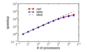
(a)

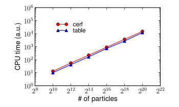
(b)

Figure 3: Plots of (b) parallel speedup versus the number of nodes, and (b) CPU time versus the number of simulation particles. cerf and table represent the weak-strong model, and look-up table model respectively.

The parallelization speedup based on the total simulation time is compared for simulations with the weak-strong model and the look-up table model. The speedup curves are very close to the ideal one below a certain number of processors, while they are less than optimal when the number of processors increases above a critical value, for example, $2^{6}$ processors. On large numbers of processors a relative fraction of the communication time in the total computing time becomes large. A parallel efficiency, defined as the speedup factor divided by the number of processors, can be obtained as high as 87% up to the critical number of processors. Though the efficiency falls well below 38% when the number of processors is beyond $2^{10}$, it runs 367 times faster than on a single processor. In order to see the scalability of our parallel code for larger problem sizes, Fig. 3 (b) shows the execution time as a function of the number of macro-particles. Here the number of processors is fixed at $2^{6}$ for all cases. It is seen that with increasing the number of simulation particles, the execution time also increases linearly.

4 Applications

In high energy storage-ring colliders, the beam-beam interactions cause emittance growth, may reduce beam lifetime, and hence limit the collider luminosity. We have used BBSIM to study beam-beam interactions and their compensations in the Tevatron, in RHIC and in the LHC.

4.1 Tevatron

The luminosity of a collider is found from

$$\mathcal{L}=\frac{N_{1}N_{2}fN_{B}}{4\pi\sigma_{x}\sigma_{y}}R$$ (36)

where $N_{1}$ and $N_{2}$ are the bunch populations of the colliding beams, $f$ the revolution frequency, $N_{B}$ the number of bunches in one beam, $\sigma_{x}$ and $\sigma_{y}$ the horizontal and vertical rms beam sizes at the collision points respectively, and $R$ the luminosity reduction factor due to the “hour-glass” effect and due to non-zero crossing angle at the interaction point. The beam-beam tune shift of beam 1 is proportional to the factor $N_{2}/\sigma_{x}\sigma_{y}$ and experience from colliders worldwide has shown that the achievable tune shift (and hence luminosity) is limited by the dynamics of the beam-beam interaction. In the Tevatron, proton and anti-proton bunches collide at two detectors called CDF and D0. They share the same beam pipe. Since the two beams circulate on helical orbits, the optics and dynamics of the beam-beam interactions are complex. The beam-beam interactions occur all around the ring and at varying betatron phases. In run II, each beam has three trains of 12 bunches [38]. Each bunch experiences 72 interactions: two interactions are the head-on collisions in the detectors. However, the other 70 interactions are long-range, and are placed at different locations for each bunch. Consequently the beam separation distances between proton and anti-proton beams at the long-range locations are different from bunch to bunch. Figure 4 shows the radial beam separation of three anti-proton bunches from the proton bunches in units of the rms beam size of the proton beam at the locations of the beam-beam interactions.

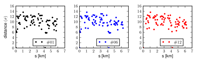
Figure 4: Separation distance between proton and anti-proton beams for anti-proton bunches #1, #6 and #12. The separation is normalized by proton beam’s rms size.

The long-range interactions of special importance are those on either side of the head-on interaction points. These occur at small separations and the beta functions there are large. It was observed that the emittance growth at the end bunches of each train is smaller than those in the middle of the train. Here we choose two end bunches (#1 and #12) and one middle bunch (#6) of the first train.

Beam emittance growth and loss rate are routinely measured during the Tevatron operation. They can be directly compared with numerical simulations but only for relatively short times. Figure 5 (a) shows the time evolution of the four-dimensional emittance of bunches #1, #6, and #12 for 15 hours of high energy physics (HEP) run of store # 7650.

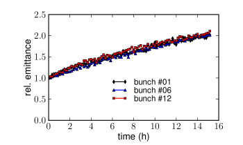
(a)

(b)

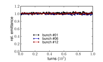
(c)

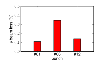
(d)

Figure 5: (a) Variation of anti-proton emittance of three bunches, #1, #6, and #12, of store #7650, (b) non-luminous loss rates of anti-proton during the first 1 hour of stores #7601-#7650, (c) simulation of anti-proton emittance growth, and (d) simulation of anti-proton beam loss. Here the emittance is plotted as $\epsilon_{4d}=\sqrt{\epsilon_{x}\epsilon_{y}}$. In the simulation, initial anti-proton emittance $\left(\epsilon_{x},\epsilon_{y}\right)$ is (9.0,7.8) mm-mrad, bunch length 1.5 nsec, and bunch intensity $0.86\times 10^{11}$. Proton’s initial emittance is (18,23) mm-mrad, bunch length 1.7 nsec, bunch intensity $2.64\times 10^{11}$. Nominal tune is (20.571, 20.569). Revolution frequency is 47.7 kHz.

The emittance is calculated and plotted by $\epsilon_{4d}=\sqrt{\epsilon_{x}\epsilon_{y}}$. It is observed that during the HEP run, the emittance growth is nearly linear. The growth rate is 6.7%/hr. Figure 5 (b) shows the measured beam loss rates of anti-proton bunches during the first 1 hour of store #7601-#7650 at collision energy 960 GeV. In order to see the effects of beam-beam interactions on the beam loss, the loss rate is obtained by subtracting the particle losses due to luminosity at the main interaction points from the total beam loss rate. Averaged loss rates of bunch #1 and #12 are 1.4 %/hr and 1.2 %/hr respectively, while the loss rate of bunch #6 is 2.3 %/hr. We performed the simulations of emittance growth and particle loss of anti-proton beam, as shown in Fig. 5 (c)-(d). The particle tracking is carried out over $10^{7}$ turns corresponding to approximately 3.5 minutes storage time of the Tevatron. In the simulation, nominal tune is (20.571, 20.569). Initial transverse (95% normalized) emittance of anti-protons $\left(\epsilon_{x},\epsilon_{y}\right)$ is set to be (9.0,7.8) mm-mrad from averaging the measured emittances while proton’s initial emittance is (18,23) mm-mrad. Bunch intensities of anti-proton and proton are $0.86\times 10^{11}$ and $2.64\times 10^{11}$ respectively. Figure 5 (c) shows the emittance growth of three bunches during the simulation. The growth rate is approximately 9 %/hr, which is close to the measured growth rate 7 %/hr in Fig. 5 (a). The emittance does not vary from bunch to bunch. However, the beam losses vary considerably from bunch to bunch. As shown in Fig. 5 (d), bunch #6 loses more particles than bunches #1 and #12, which agrees well with the observation. For the simulation of beam loss, we used the hollow Gaussian distribution in transverse action coordinates. Most of the lost particles have large transverse actions as shown in Fig. 6 (a), while the lost particles are distributed over the entire range of longitudinal action, as shown in Fig. 6 (b).

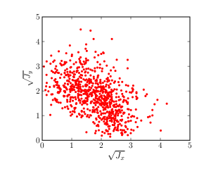
(a)

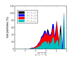
(b)

Figure 6: (a) Scatter plot of lost particles in action space $\left(\sqrt{J_{x}},\sqrt{J_{y}}\right)$ and (b) plot of lost particles versus $\sqrt{J_{x}+J_{y}}$ for different longitudinal action. The axis variables are normalized by rms size of transverse action.

The compensation of long-range effects in the Tevatron with a current-carrying wire was investigated using an earlier version of the code [8]. It was found that a single wire was unable to compensate for all the 70 interactions, since they were all at different betatron phases from the wire.

4.2 Relativistic Heavy Ion Collider

We have studied the effects of a current-carrying wire on the beam dynamics in RHIC [32]. Two current-carrying wires, one for each beam, have been installed between the magnets $Q3$ and $Q4$ of IP6 in the RHIC tunnel. In the physics run 9, an attempt was made to compensate the long range beam-beam interaction which shows the reduction of beam loss [39]. During the physics run 7 and 8, the impact of current-carrying wires on a beam was measured without an attempt to compensate the beam-beam interactions. However, the experimental results help to understand the beam-beam effects because the wire force is similar to the long-range beam-beam force at large separations. As an example, Fig. 7 plots the beam loss rate due to the wire as a function of beam-wire separation distance.

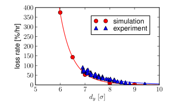
(a)

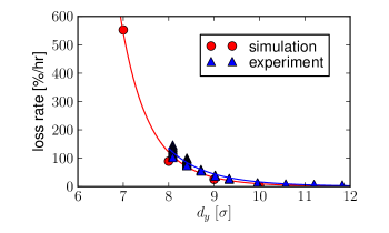
(b)

Figure 7: Comparison of the simulated beam loss rates with the measured as a function of separations. (a) gold beam at collision energy, (b) deuteron beam at collision energy [32].

The onset of beam losses is observed at 8 $\sigma$ and 9 $\sigma$ for gold and deuteron beams, respectively. The threshold separation for the onset of sharp losses observed in the measurements and simulations agree to better than 1 $\sigma$. It is also significant that the simulated loss rates at 7 and 8 $\sigma$ separation for the gold beam and 8 and 9 $\sigma$ for the deuteron beam are very close to the measured loss rates. At fixed separation, the wire causes a much higher beam loss with the deuteron beam than with the gold beam. The loss rate for the gold beam at a 8 $\sigma$ separation is about 10 %/hr while for the deuteron beam the loss rate is about an order of magnitude higher both in measurements and simulation. Simulations of the beam loss rate when the wire is present are in good agreement with the experimental observations.

In the proton-proton runs of RHIC, the maximum beam-beam parameter reached so far is about $\xi=0.008$. This tune shift is large enough that the combination of beam-beam and machine nonlinearities excite betatron resonances which cause emittance growth and diffuse particles into the tail of beam distribution and beyond. Consequently RHIC is actively developing an electron lens for compensating the head-on interactions [40]. In order to seek the electron lens parameters at which the beam life time is improved, we choose three different electron beam distribution functions: (a) $1\sigma$ Gaussian distribution with the same rms beam size as that of the proton beam $\sigma$, (b) $2\sigma$ Gaussian distribution with rms size twice that of the proton beam, and (c) Smooth-edge-flat-top (SEFT) distribution with an edge around at 4 $\sigma$. When the electron beam profile matches the proton beam, the full compression of the tune spread requires the electron beam intensity $N_{e}=4\times 10^{11}$ which is defined as the electron beam intensity required for full compensation. Table 1 shows the results of particle loss for different intensities with the three electron beam profiles.

Profile	Intensity $\left(4\times 10^{11}\right)$	Particle loss†(%)
$1\sigma$ Gaussian	1	635
	1/2	115
	1/4	63
	1/8	30
$2\sigma$ Gaussian	4	93
	2	10
	1	8
	1/2	6
SEFT	8	330
	4	21
	2	22
	1	6
	1/2	6
†relative to that without beam-beam compensation

Table 1: Comparison of particle loss for different electron beam profiles and intensities.

At an intensity $N_{e}=4\times 10^{11}$, the particle loss is nearly six times the loss without beam-beam compensation. The beam lifetime at $N_{e}=2\times 10^{11}$ however is comparable with that of no beam-beam compensation. As the electron beam intensity is decreased, the particle loss decreases significantly, and is reduced to 30% of that without beam-beam compensation at $N_{e}=0.5\times 10^{11}$. For the $2\sigma$ Gaussian and SEFT electron beam profiles, we calculated particle loss for different electron beam intensities. The upper limits of the electron beam intensity for these two distributions are chosen so that peak of the electron profile matches that of the full compensation at $1\sigma$ Gaussian. For the intensities $2\times 10^{11}$ and $4\times 10^{11}$ of $2\sigma$ Gaussian profile, there is a significant reduction in beam loss, for example, below 10% of the particle loss without beam-beam compensation when the electron beam intensity is $2\times 10^{11}$. A significant improvement of beam lifetime with the SEFT profile is also observed below $8\times 10^{11}$. There is a threshold electron beam intensity below which beam life time is increased: $2\times 10^{11}$ for the $1\sigma$ Gaussian, $8\times 10^{11}$ for the $2\sigma$ Gaussian, and $16\times 10^{11}$for the SEFT profile. Particle loss is relatively insensitive to electron lens current variations below the threshold current with the $2\sigma$ Gaussian and SEFT profiles. This looser tolerance on the allowed variations in electron intensity will allow greater intensity fluctuations and is likely to be beneficial during experiments.

4.3 Large Hadron Collider

As mentioned above, long-range beam-beam interactions cause emittance growth or beam loss in the Tevatron and are expected to deteriorate beam quality in the LHC. Increasing the crossing angle to reduce their effects has several undesirable effects, the most important of which is a lower luminosity due to the smaller geometric overlap. For the LHC, a wire compensation scheme has been proposed to compensate the long-range interactions [23]. However, several issues need to be resolved for efficient compensation. With the design bunch spacing, there are about 30 long-range interactions on both sides of an interaction point (IP). The beam-beam separation distance varies from 6.3 $\sigma$ to 12.6 $\sigma$. The resulting beam-beam force is not identical to that generated by a single or multiple wire(s) but can be closely approximated by the wires. Unlike the Tevatron, the long-range forces in the LHC are all at nearly the same betatron phase and this makes the compensation scheme feasible. The wire-beam separation distance is one of the parameters which determine the performance of a wire compensator. Figure 8 (a) shows the beam-beam separation distance normalized by the transverse rms bunch size. Two counter-rotating beams collide at a vertical crossing angle near IP1 while they collide at a horizontal crossing angle near IP5. The separations are asymmetric with respect to the interaction points. The reference wire-beam separation (9 $\sigma$) is chosen as the average of beam-beam separations.

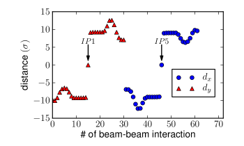
(a)

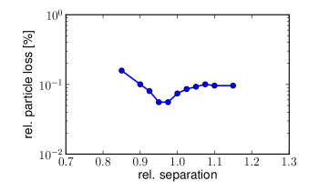
(b)

Figure 8: Plot of (a) beam-beam separation at IP 1 and 5 and (b) particle loss according to wire separation distance with wire strength 82.8 Am.

Figure 8 (b) shows the results of particle loss for different wire-beam separations. The particle loss saturates at large separation while there is a sharp increase of particle loss at small separation. We directly see the minimum particle loss between 0.9 and 1.0 of the reference separation. It reveals that the average of beam-beam separations is close to an optimal separation between the wire and the high energy bunch.

5 Summary

In this paper, an efficient parallel beam simulation model for circular colliders is presented in order to study the effects of beam-beam interactions and machine nonlinearities, and the effectiveness of beam-beam compensation schemes. We have included the major nonlinearities present in accelerators in our program as well as models for several methods to compensate the effects of beam-beam interactions. A particle-domain decomposition scheme is implemented with the master/slave configuration to achieve a balanced workload in a parallel environment. A performance test of beam-beam interactions indicates that the parallelization scheme scales linearly in both the number of processors and the number of particles in the beam. We have used the program to study the emittance growth and beam loss of different bunches due to the beam-beam interactions in the Tevatron, the compensation of head-on beam-beam interactions with a low energy electron beam in RHIC, and the long-range beam-beam compensation using a current-carrying wire in the Tevatron, RHIC and the LHC. The pattern of beam losses observed in the Tevatron is reproduced in the simulations. In RHIC, simulations of the beam loss rate when the wire is present are in good agreement with the experimental observations. We have several predictions from the results of head-on compensation in RHIC. For example we find that proton beam life time is increased if the electron beam intensity is kept below a threshold intensity. An electron beam wider than the proton beam at the electron lens location is found to increase beam life time. The results of LHC simulation with the current carrying wire show that the particle loss is minimized when the beam-wire separation is close to the average of beam-beam separations.

6 Acknowledgments

We thank V. Boocha, B. Erdelyi and V. Ranjbar for their contributions to the development of BBSIM. This research used resources of the Accelerator Physics Center at Fermi National Accelerator Laboratory as well as resources of the National Energy Research Scientific Computing Center at Lawrence Berkeley National Laboratory, which is supported by the Office of Science of the U.S. Department of Energy. This work is partially supported by the US Department of Energy through the US LHC Accelerator Research Program (LARP). Fermi National Accelerator Laboratory (Fermilab) is operated by Fermi Research Alliance, LLC under Contract No. DE-AC02-07CH11359 with the United States Department of Energy.

References

- [1] J.-Y. Hemery, A. Hofmann, J.-P. Koutchouk, S. Myers, L. Vos, Investigation of the coherent beam-beam effects in the ISR, IEEE T. Nucl. Sci. NS-28 (1981) 2497.
- [2] L. Evans, J. Gareyte, M. Meddahi, R. Schmidt, Beam-beam effects in the strong-strong regime at the CERN-SPS, in: Proceedings of the 1889 Particle Accelerator Conference, 1989.
- [3] W. Fischer, A. Drees, J. Brennan, R. Connolly, R. Fliller, S. Tepikian, J. van Zeijts, Beam lifetime and emittance growth measurements of gold beams in RHIC at storage, in: Proceedings of the 2001 Particle Accelerator Conference, 2001, p. 21.
- [4] T. Sen, B. Erdelyi, M. Xiao, V. Boocha, Beam-beam effects at the Fermilab Tevatron: Theory, Phys. Rev. Spec. Top. Acceler. Beams 7 (2004) 041001.
- [5] F. Zimmermann, Beam-beam effects in the Large Hadron Collider, in: D. Rice (Ed.), ICFA Beam Dynamics Newsletter, no. 34, 2004, p. 26.
- [6] V. Shiltsev, Y. Alexahin, V. Lebedev, P. Lebrun, R. S. Moore, T. Sen, A. Tollestrup, A. Valishev, X. L. Zhang, Beam-beam effects in the Tevatron, Phys. Rev. Spec. Top. Acceler. Beams 8 (2005) 101001.
- [7] J. Beebe-Wang, S. Y. Zhang, Observation and simulation of beam-beam induced emittance growth in RHIC, in: Proceedings of the 2009 Particle Acclerator Conference, 2009, p. 2622.
- [8] T. Sen, B. Erdelyi, Feasibility study of beam-beam compensation in the Tevatron with wires, in: Proccedings of the 2005 Particle Accelerator Conference, 2005, p. 2645.
- [9] F. Zimmermann, J.-P. Koutchouk, F. Roncarolo, J. Wenninger, T. Sen, V. Shiltsev, Y. Papaphilippou, Experiments on LHC long-range beam-beam compensation and crossing schemes at the CERN SPS in 2004, in: Proceedings of the 2005 Particle Accelerator Conference, 2005, p. 686.
- [10] H. J. Kim, T. Sen, N. P. Abreu, W. Fischer, Simulations of beam-beam and beam-wire interactions in RHIC, Phys. Rev. Spec. Top. Acceler. Beams 12 (2009) 031001.
- [11] http://www-ap.fnal.gov/hjkim.
- [12] Message Passing Interface Forum, U. of Tennessee, Knoxbille, TN, MPI-2: Extenstions to the Message-Passing Interface (2003).
- [13] S. Balay, J. Brown, K. Buschelman, V. Eijkhout, W. D. Gropp, D. Kaushik, M. G. Knepley, L. C. McInnes, B. Smith, H. Zhang, PETSc Users Manual, Tech. Rep. ANL-95/11 - Revision 3.0.0, Argonne National Laboratory (2008).
- [14] NCSA, UIUC, Urbana, IL, HDF5 User’s Guide (2005).
- [15] K. Hirata, H. Moshammer, F. Ruggiero, A symplectic beam-beam interaction with energy change, Part. Accel. 40 (1993) 205.
- [16] K. Wille, The Physics of Particle Accelerators: an introduction, Oxford University Press, 2000.
- [17] L. C. Teng, Concerning n-dimensional coupled motions, Tech. Rep. FN-229, FNAL (1971).
- [18] M. Bassetti, G. A. Erskine, Closed expression for the electrical field of a two-dimensional Gaussian charge, Tech. Rep. CERN-ISR-TH/80-06, CERN (1980).
- [19] R. W. Hockney, The potential calculation and some applications, Meth. Comput. Phys. 9 (1970) 135–211.
- [20] J. Qiang, M. A. Furman, R. D. Ryne, Strong-strong beam-beam simulation using a green function approach, Phys. Rev. Spec. Top. Acceler. Beams 5 (2002) 104402–1.
- [21] K. Hirata, Don’t be afraid of beam-beam interactions with a large crossing angle, Tech. Rep. SLAC-PUB-637, SLAC (1994).
- [22] L. H. A. Leunissen, F. Schmidt, G.Ripken, Six-dimensional beam-beam kick including coupled motion, Phys. Rev. Spec. Top. Acceler. Beams 3 (2000) 124002.
- [23] J.-P. Koutchouk, Principle of a correction of the long-range beam-beam effect in LHC using electromagnetic lenses, Tech. Rep. LHC Project Note 223, CERN (2000).
- [24] E. Tsyganov, R. Meinke, W. Nexen, A. Zinchenko, Compensation of the beam-beam effect in proton-proton colliders, Tech. Rep. SSCL-Preprint-519, SSCL (1993).
- [25] V. Shiltsev, V. Danilov, D. Finley, A. Sery, Considerations on compensation of beam-beam effects in the tevatron with electron beams, Phys. Rev. Spec. Top. Acceler. Beams 2 (1999) 071001.
- [26] V. Shiltsev, Y. Alexahin, K. Bishofberger, V. Kamerdzhiev, V. Parkhomchuk, V. Reva, N. Solyak, D. Wildman, X.-L. Zhang, F. Zimmermann, Experimental studies of compensation of beam-beam effects with Tevatron electron lenses, New J. Phys. 10 (2008) 043042.
- [27] R. B. Palmer, Energy scaling, crab crossing and the pair problem, Tech. Rep. SLAC-PUB-4707, SLAC (1988).
- [28] K. Oide, K. Yokoya, Beam-beam collision scheme for storage-ring colliders, Phys. Rev. A: At., Mol., Opt. Phys. 40 (1) (1989) 315–316.
- [29] B. Erdelyi, T. Sen, Compensation of beam-beam effects in the tevatron with wires, Tech. Rep. Fermilab-TM-2268-AD, Fermilab (2004).
- [30] C. K. Birdsall, A. B. Langdon, Plasma Physics via Computer Simulation, McGraw-Hill, New York, 1985.
- [31] T. Sen, J. A. Ellison, Diffusion due to beam-beam interaction and fluctuating fields in hadron colliders, Phys. Rev. Lett. 77 (6) (1996) 1051–1054.
- [32] H. J. Kim, T. Sen, N. P. Abreu, W. Fischer, Studies of wire compensation and beam-beam interaction in rhic, in: Proceedings of the 11th European Particle Accelerator Conference, 2008, p. 3119.
- [33] R. Bartolini, A. Bazzani, M. Giovannozzi, W. Scandale, E. Todesco, Tune evaluation in simulations and experiments, Tech. Rep. SL/95-84, CERN (1995).
- [34] J. Borer, G. Guignard, A. Hofmann, E. Peschardt, F. Sacherer, B. Zotter, Information from beam response to longitudinal and transverse excitation, IEEE T. Nucl. Sci. NS-26 (1979) 3405–3408.
- [35] J. Laskar, Frequency analysis for multi-dimensional systems. global dynamics and diffusion, Physica D 67 (1993) 257–281.
- [36] R. W. Hockney, J. W. Eastwood, Computer Simulation Using Particles, Taylor & Francis, Inc., 1988.
- [37] M. J. Quinn, Parallel Programming in C with MPI and OpenMP, McGraw-Hill, 2004.
- [38] Run II Handbook, http://www-bd.fnal.gov/runII/index.html.
- [39] R. Calaga, W. Fischer, G. Robert-Demolaize, RHIC BBLR measurement in 2009, in: Proceedings of the 2010 International Particle Accelerator Conference, 2010, p. 510.
- [40] W. Fischer, et al., Status of RHIC head-on beam-beam compensation project, in: Proceedings of the 2010 International Particle Accelerator Conference, 2010, p. 513.