A Panorama on Multiscale Geometric Representations,
Intertwining Spatial, Directional and Frequency Selectivity

Abstract

The richness of natural images makes the quest for optimal representations in image processing and computer vision challenging. The latter observation has not prevented the design of image representations, which trade off between efficiency and complexity, while achieving accurate rendering of smooth regions as well as reproducing faithful contours and textures. The most recent ones, proposed in the past decade, share an hybrid heritage highlighting the multiscale and oriented nature of edges and patterns in images. This paper presents a panorama of the aforementioned literature on decompositions in multiscale, multi-orientation bases or dictionaries. They typically exhibit redundancy to improve sparsity in the transformed domain and sometimes its invariance with respect to simple geometric deformations (translation, rotation). Oriented multiscale dictionaries extend traditional wavelet processing and may offer rotation invariance. Highly redundant dictionaries require specific algorithms to simplify the search for an efficient (sparse) representation. We also discuss the extension of multiscale geometric decompositions to non-Euclidean domains such as the sphere or arbitrary meshed surfaces. The etymology of panorama suggests an overview, based on a choice of partially overlapping “pictures”. We hope that this paper will contribute to the appreciation and apprehension of a stream of current research directions in image understanding.

Keywords: Review, Multiscale, Geometric representations, Oriented decompositions, Scale-space, Wavelets, Atoms, Sparsity, Redundancy, Bases, Frames, Edges, Textures, Image processing, Haar wavelet, non-Euclidean wavelets.

 

 

1 Introduction: Vision Aspects, Scope and Notations

1.1 Background on Vision Aspects of Scale

Many natural-world object features are substantive only over a certain spatial extent. In other words, the scale of observation is crucial in object recognition and understanding. For instance, a chair would be easily recognizable in the scale of a few meters. But neither at a centimeter scale which captures the chair’s texture and not its object appearance, or at a hectometer scale, where the chair’s appearance is hardly distinguished from other surrounding objects.

Accordingly, early neurophysiological studies in biologic perception reveal that those objects are generally apprehended differently according to the scale of observation by the sensory receptors and the cortex of mammalians [1, 2]. Efficient information extraction is thus required for artificial sensing systems to mimic standard biologic tasks such as object recognition.

Pixel-based representations as linear combinations of “delta” functions suffice for simple data manipulation but are very limited for higher level tasks. Only assuming some sufficient resolution in the data, the lack of prior knowledge in the extent of objects to be analyzed calls for tools able to unveil the appropriate scales and to allow a hierarchical representation of the underlying features [3, 4, 5]. Disregarding the peculiar fractal formalism [6, 7] where similar phenomena appear at different scales (what is called self-similarity), special attention has been paid to data transformations able to capture object features over a range of scales in a more compact form. Sparsity, amounting to a reduced number of parameters in a suitable domain, is thus used as a heuristic guide to image understanding. Bearing analogies with findings in vision processes [8], several sparse decompositions have proven efficient in image compression, with the discrete wavelet transform (DWT) as their most well-known avatar, often intermingled with information theory and technical wizardry, from bit plane arithmetic coding [9] to trellis coded quantization. A compact history and a paper collection are given in [10, 11], respectively.

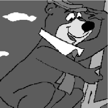
(a)

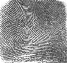
(b)

Figure 1: Two faces of the cartoon-texture model: (a) Yogi bear (b) Fingerprint.

Yet, beyond image compression transforms, other decomposition techniques are needed, with more resolving power in complex scene detection, denoising, segmentation or, in a broad sense, scene understanding. As a matter of fact, standard separable wavelet transforms appropriately detect point-like ($0$-D) singularities and address mild noise levels. Still they generally lack performance in dealing with higher dimensional features combining both regularity and singularity such as edges, contours or regular textures, that may also be anisotropic. Amongst their limitations are shift sensitivity, limited orientation selectivity, rigid and uneven atom shapes (e.g., fractal-looking asymmetric Daubechies wavelets), crude frequency direction selection. Major challenges reside in a proper definition of the underlying regularity (with respect to each feature) and corresponding singularities. These challenges are amplified by additional degradations from which acquired data may suffer such as blur, jitter and noise. Descriptive mathematical models of images combining cartoon and textures become increasingly popular [12, 13] and progressively yield tractable algorithms. We note that there exists a continuum of real-world images between cartoon and textures, ranging from cartoon-ish Yogi bear in Fig. 1(a) to “textural” fingerprints in Fig. 1(b). In between these two extreme image types, there exists many possible variations in image object complexity.

Moreover, both contours and (even regular) textures are known to be ill-defined. They are indeed viewer- and scale-dependent concepts in discrete images or volumes. Consider an image resulting from a combination of piecewise smooth components, contours, geometrical textures and noise. Their discrimination is required for high level image processing tasks. Each of these four components could be detected, described and modeled by different formalisms: smooth curves or polynomials, oriented regularized derivatives, discrete geometry, parametric curve detectors (such as the Hough transform), mathematical morphology, local frequency estimators, optical flow approaches, smoothed random models, etc. They have progressively influenced the hybridization of standard multiscale transforms towards more geometric and sparser representations of such components, with improved localization, orientation sensitivity, frequency selectivity or noise robustness.

1.2 Scope of the Paper

Geometry driven “$\star$-let” transforms [14] have been popular in the past decade, with a seminal ancestor in [15]. Early [16], a debate opened on the relative strength of Eulerian (non-adaptive) versus Lagrangian (adaptive) representation, now pursued with the growing interest in dictionary learning [17].

As of today, the authors believe that the discussion is not fully settled in the various different uses of sparsity in images. Neither has the trade-off between redundancy and sparsity. A number of early papers on geometric multiscale methods appear in [18]. Comparisons are drawn in [19, 20], while [21, 22, 23, 22, 24] focus on ridgelets, curvelets and wedgelets, as representative of fixed and adaptive decompositions. The present paper aims at providing a broader panorama of the recent developments in multiscale decompositions targeted to efficient representation of geometric features in images: smooth content (multiscale or hierarchical), edges and contours (locally spatial) and textures (locally spectral). We emphasize the main characteristics and differences pertaining to spatial, directional and frequency selectivity of the selected methods. The paper therefore cites a dense set of references, ranging from continuous to discrete representations, from (nearly) orthogonal to (fully) redundant. As a guiding thread to this panorama, we illustrate some of the reviewed geometric multiscale decompositions on a memorial plaque in Szeged University, Hungary, depicted in Fig. 2. It features simple objects (embedded rectangles and a disk), a few differently oriented features and regular textures at different scales. Since some of the illustrations have been slightly enhanced to improve the clarity of details, they are available in original resolution online [26]. This picture finally honors Alfréd Haar’s originative paper [27] Zur Theory der orthogalen Funktionen Systeme (On the Theory of Orthogonal Function Systems) and his eponymous wavelet. He also founded Acta Scientiarum Mathematicarum together with Frigyes Riesz, whose works percolated wavelet theory [28].

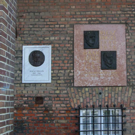
Figure 2: Szeged University Memorial plaque in honor of A. Haar and F. Riesz: A szegedi matematikai iskola világhírű megalapítói (The world-wide famous founders of the mathematical school in Szeged).

The paper is organized as follows: the remaining of Section 1 is devoted to context and notations for image representations. Then, as a preliminary to geometric tools, a quick survey of early multiscale decompositions is presented in Section 2. More recent transforms, termed directional or geometrical, circumventing aforementioned drawbacks, are discussed in Section 3. Owing to the additional degrees of freedom provided by these representations, a discussion is carried out in Section 4 on redundancy and adaptivity. The extension of frequency, scale and directionality to non-Euclidean spaces or grids such as the sphere, are presented in Section 5. Finally, concluding remarks are given in Section 6.

1.3 Mathematical Framework

1.3.1 Notations and Conventions

This paper describes numerous mathematical methods designed for different spaces and geometries. We have tried therefore to adopt coherent representations for the many mathematical notions that coexist in this text. For instance, functions and vectors in high dimensional spaces are generally referring to some signal of interest (e.g., $1$-D signals or images). They must therefore share the same notations and we thus decided to write them as simple lowercase Roman or Greek letters. However, coordinate systems, vectors in 2 or 3 dimensions and multi-indices are denoted in bold symbols.

The (Hilbert) space $\mathbb{L}^{2}(\mathcal{X})$ is the space of square integrable functions on the space $\mathcal{X}$, i.e., given the (Lebesgue) integration measure ${\rm d}\rho$ on that space, $\mathbb{L}^{2}(\mathcal{X})=\mathbb{L}^{2}(\mathcal{X},{\rm d}\rho)=\{f:\mathcal{X}\to\mathbb{C}:\|f\|^{2}:=\int_{\mathcal{X}}\ |f(\boldsymbol{u})|^{2}\,{\rm d}\rho(\boldsymbol{u})<\infty\}$. In $\mathbb{L}^{2}(\mathcal{X})$ the inner product between two functions $g,h\in\mathbb{L}^{2}(\mathcal{X})$ is denoted by $\langle g,h\rangle=\int_{\mathcal{X}}g^{*}(\boldsymbol{u})\,h(\boldsymbol{u})\ {\rm d}\rho(\boldsymbol{u})$ with ^∗ the complex conjugation. By extension, for $p\geqslant 1$, we also use the (Banach) spaces $\mathbb{L}^{p}(\mathcal{X})=\mathbb{L}^{p}(\mathcal{X},{\rm d}\rho)=\{f:\mathcal{X}\to\mathbb{C}:\|f\|_{p}^{p}:=\int_{\mathcal{X}}\ |f(\boldsymbol{u})|^{p}\,{\rm d}\rho(\boldsymbol{u})<\infty\}$, with $\|\!\cdot\!\|_{2}=\|\!\cdot\!\|$.

We also use some discrete spaces as the common $\ell^{p}_{N}=(\mathbb{C}^{N},\|\cdot\|_{p})$ with $\|v\|^{p}_{p}:=\sum_{i}|v_{i}|^{p}$ for $p\geqslant 1$ and $v\in\mathbb{C}^{N}$, with again the shorthand $\|\!\cdot\!\|=\|\!\cdot\!\|_{2}$. In $\ell^{2}_{N}$, the inner product between $u,v\in\ell^{2}_{N}$ is written $\langle u,v\rangle=u\cdot v=\sum u_{i}^{*}v_{i}$. Whether the overused notations $\langle\cdot,\cdot\rangle$ or $\|\!\cdot\!\|_{p}$ are applied to continuous or discrete mathematical objects will remain clear from the context. The spaces $\ell^{p}$ are the generalization of the previous finite spaces to infinite sequences, i.e., $\ell^{p}=\{v=(v_{i})_{i\in\mathbb{N}}:\|v\|^{p}_{p}=\sum_{i\geqslant 0}|v_{i}|<\infty\}$.

For functions $f\in\mathbb{L}^{2}(\mathcal{X})$ or discrete sequences $v\in\ell^{2}_{N}$, $\hat{f}$ and $\hat{v}$ denote the Fourier transform of $f$ or $v$ respectively. For instance, for $\mathcal{X}=\mathbb{R}$ and $f\in\mathbb{L}^{2}(\mathbb{R})$, $\hat{f}(\omega)={\textstyle\frac{1}{\sqrt{2\pi}}}\int_{\mathbb{R}}f(t)\,e^{-{\rm i}\omega t}\ {\rm d}t$ and $f(t)={\textstyle\frac{1}{\sqrt{2\pi}}}\int_{\mathbb{R}}\hat{f}(\omega)\,e^{{\rm i}\omega t}\ {\rm d}\omega$ are the Forward and Inverse Fourier transform respectively. For $f\in\mathbb{L}^{2}(\mathbb{R}^{2})$ and $\boldsymbol{x},\boldsymbol{\omega}\in\mathbb{R}^{2}$, the same transforms are $\hat{f}(\boldsymbol{\omega})={\textstyle\frac{1}{{2\pi}}}\int_{\mathbb{R}^{2}}f(\boldsymbol{x})\,e^{-{\rm i}\boldsymbol{\omega}\cdot\boldsymbol{x}}\ {\rm d}^{2}\boldsymbol{x}$ and $f(\boldsymbol{x})={\textstyle\frac{1}{{2\pi}}}\int_{\mathbb{R}^{2}}\hat{f}(\boldsymbol{\omega})\,e^{{\rm i}\boldsymbol{\omega}\cdot\boldsymbol{x}}\ {\rm d}^{2}\boldsymbol{\omega}$. For $v\in\ell^{2}_{N}$, the same transforms are $\hat{v}_{k}=\frac{1}{\sqrt{N}}\,\sum_{j}v_{j}\exp(-2\pi{\rm i}\,jk/N)$ and $v_{j}=\frac{1}{\sqrt{N}}\,\sum_{k}\hat{v}_{k}\exp(2\pi{\rm i}\,jk/N)$. In matrix algebra notations, this can be rewritten as $v=\mathcal{F}\hat{v}$ and $\hat{v}=\mathcal{F}^{*}v$, where the Fourier matrix $\mathcal{F}\in\mathbb{C}^{N\times N}$ is given by $\mathcal{F}_{jk}=\frac{1}{\sqrt{N}}\exp(2\pi{\rm i}\,jk/N)$, and $\mathcal{F}^{*}$ is its complex adjoint. The convolution by time-invariant filter $h$ operates as $(f\star h)(t)=\int_{-\infty}^{\infty}f(u)h^{*}(t-u){\rm d}u$ and $(v\star h)_{n}=\sum_{n^{\prime}}h^{*}_{n^{\prime}}v_{n-n^{\prime}}$ in continuous and discrete sample domain respectively. The ubiquitous Gaussian kernel with scale parameter $\sigma>0$ is denoted by $G_{\sigma}(\boldsymbol{x})=\exp(-{\textstyle\frac{1}{2\sigma^{2}}}\|\boldsymbol{x}\|^{2})$, with $G(\boldsymbol{x})=G_{1}(\boldsymbol{x})$.

1.3.2 Image Representations in Bases and Frames

Stability and Frames

This paper describes processing methods that make use of a decomposition of the image $f\in\mathbb{L}^{2}([0,1]^{2})$ into a family of atoms $\mathcal{B}=\{\psi_{\boldsymbol{m}}\}_{\boldsymbol{m}}$. Each atom $\psi_{\boldsymbol{m}}\in\mathbb{L}^{2}([0,1]^{2})$ is parameterized by a multi-index $m$ (that might take into account its frequency, position, scale and orientation). Numerical processing is performed on discretized images which are vectors $f\in\mathbb{R}^{N}$, where $N$ stands for the number of pixels. The atoms of $\mathcal{B}$ are also discretized and the continuous inner products are replaced by the standard discrete inner product in $\mathbb{R}^{N}$.

To guarantee a stable reconstruction from the coefficients $\{\langle\psi_{\boldsymbol{m}},\,f\rangle\}_{\boldsymbol{m}}$, the family $\mathcal{B}$ is assumed to be a frame [29, 30, 28, 31, 32] of $\mathbb{L}^{2}([0,1]^{2})$ or $\mathbb{R}^{N}$, which means that there exist two constants $0<\mu_{1}\leqslant\mu_{2}<\infty$ such that for all $f$

$$\mu_{1}\|f\|^{2}\leqslant\sum_{\boldsymbol{m}}|\langle\psi_{\boldsymbol{m}},\,f\rangle|^{2}\leqslant\mu_{2}\|f\|^{2}.$$ (1)

Atoms are allowed to be linearly dependent, thus corresponding to a redundant representation. Redundancy enables atoms to meet certain additional constraints, for instance smoothness, symmetry and invariance to translation or rotation.

Thresholding for Approximation and Processing

Using a dual frame $\{\tilde{\psi}_{\boldsymbol{m}}\}_{\boldsymbol{m}}$ [28], an image is recovered from the set of coefficients as $f=\sum_{\boldsymbol{m}}\langle\psi_{\boldsymbol{m}},\,f\rangle\tilde{\psi}_{\boldsymbol{m}}$. The computation of the set of coefficients $\{\langle\psi_{\boldsymbol{m}},\,f\rangle\}_{\boldsymbol{m}}$ for a discrete image $f\in\mathbb{R}^{N}$ is usually performed using a fast algorithm, that also enables a fast reconstruction of an image from coefficients.

The basic processing operation, used in denoising and compression applications, is the thresholding

$$f_{M}=H_{T}(f,\mathcal{B})=\sum_{\boldsymbol{m}\ :\ |\langle\psi_{\boldsymbol{m}},\,f\rangle|>T}\langle\psi_{\boldsymbol{m}},\,f\rangle\ \tilde{\psi}_{\boldsymbol{m}}$$ (2)

where $M=\#\left\{\boldsymbol{m}\,:\;|\langle\psi_{\boldsymbol{m}},\,f\rangle|>T\right\}$ counts the number of non-zero coefficients in (2).

When $\mu_{1}=\mu_{2}$, the frame is said to be tight (Parseval tight frame). If furthermore $\mu_{1}=\mu_{2}=1$, then one can choose $\tilde{\psi}_{\boldsymbol{m}}=\psi_{\boldsymbol{m}}$, and $\mathcal{B}=\{\psi_{\boldsymbol{m}}\}_{\boldsymbol{m}}$ is then an orthonormal basis if $\|\psi_{\boldsymbol{m}}\|=1$ for all $\boldsymbol{m}$. In this last case, $\mathcal{B}$ performs the least energy reconstruction of $f_{M}$ in (2), or equivalently, $f_{M}$ is the best $M$-terms approximation of $f$. The decay of the approximation error $\|f-f_{M}\|$ is related to both the average risk of a denoiser, and the distortion rate decay of a coder, see for instance [33]. This motivates the search for bases or frames $\mathcal{B}$ which can efficiently approximate large classes of (natural) images. When the frame is redundant, more complicated decomposition methods improve the sparsity of the representation (see Sec. 4.1).

2 Early Scale-Related Representations

2.1 Frequency, Heat Kernel and Scale-Space Formalism

At the heart of modern signal processing techniques is the concept of signal representation, i.e., the selection of an efficient “point of view” in the study of signal properties that is not restricted to straightforward spatial descriptions.

The most obvious alternative signal representation is its frequency reading, i.e., the one provided by the Fourier transform of the signal explained in Sec. 1.3.1 [34, 35]. However, this representation is not sufficiently “local”. It is indeed rather difficult to detect what spatial part of an image contributes to high peaks in the Fourier spectrum. Fig. 3 represents the amplitude spectrum of the luminance component from Fig. 2. It exhibits a mixture of prominent vertical and horizontal directions with tiny fuzzy diagonal ones.

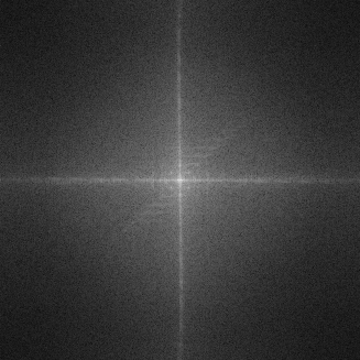
Figure 3: Magnitude of the $2$-D Fourier transform of the Haar-Riesz Memorial plaque in Fig. 2.

An approach for obtaining a better localization is to introduce a notion of “scale” in the image observation. This has been performed very early in image and signal processing by either windowing or introducing scales in the Fourier transform [36, 37] or observing a well-known diffusion process like the heat dynamics governed by the famous Heat equation. The idea relies on considering the image as an initial configuration of heat that is diffused with a time variable $\tau>0$ and in interpreting this time parameter as the “scale”. Indeed, in this dynamic diffusion, small image structures will be smoothed early at small evolution time while larger ones persist for a larger duration. Interestingly, this diffusion is equivalently described by a filtering process: the convolution of the image by a Gaussian function $G_{\sigma}$ of width $\sigma=\sqrt{2\tau}$ [38, 39, 40]. This image unfolding into a scale-space domain has led to many new image processing techniques such as edge, ridge and feature detection [41, 42]. This is illustrated in Fig. 4, where the original image is convolved with three different Gaussian kernels in dyadic progression. Large objects such as the white rectangular plaques persist across all scales, while brick and grid textures vanish in Fig. 4(c). The overall redundancy of the Gaussian pyramid is given by the number of smoothing kernels. Taking advantage of the resolution loss, the redundancy factor may be reduced by sub-sampling, leading to the “Gaussian pyramid” construction.

(a)

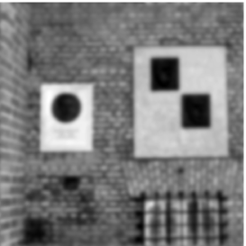
(b)

(c)

Figure 4: Gaussian scale-space decomposition of the Haar-Riesz Memorial plaque at three different scales.

The scale content of the image can be decomposed further by computing, for instance, differences between two filterings performed at two different scales. This led to the famous Littlewood-Paley decomposition, or to the (invertible) Laplacian pyramid conveniently combining multiple sub-sampled low-pass filterings of images, creating a pyramidal scale hierarchy [43]. Interestingly, the resulting decomposition represented in Fig. 5 is a complete image representation that can advantageously be processed before reconstructing a new “restored” image (e.g., in image denoising). Additionally, image singularities are enhanced at fine scales, with low activity regions associated with coefficients being close to zero. Fast implementations of deformable (steerable or scalable) decompositions [44] are available for instance with recursive filters [45] or efficient multirate filter banks [46, 47, 48, 49].

Figure 5: Laplacian pyramid decomposition of the Haar-Riesz Memorial plaque.

Remarkably, the notion of Scale-Space has been defined and “axiomatized” more than 50 years ago by the Japanese mathematicians Iijima and Otsu, as presented in [50]. As we will realize throughout this paper, this scale-space representation (refer to [51] for a recent overview and axiomatic generalization) was the starting point of many new ways to represent images.

2.2 Isotropic Continuous Wavelet Transform

The continuous wavelet transform somehow generalizes the previous scale-space formalism driven by the Gaussian kernel to any “function” with enough regularity. The continuous wavelet transform was initially developed for the transformation of $1$-D signals [52] and further extended in $2$-D first with isotropic wavelets. The case of non-isotropic (directional) wavelets was defined later [53] (see Sec. 3.2.3).

In one dimension, a wavelet $\psi$ is an integrable and well-localized function of $\mathbb{L}^{2}(\mathbb{R})$, generally described as locally oscillating, i.e., $\int_{\mathbb{R}}\psi(t){\rm d}t=0$. It may be dilated or contracted by a scale factor $a>0$ and translated to a position $b\in\mathbb{R}$: $\psi_{(b,a)}(t)=\tfrac{1}{\sqrt{a}}\,\psi(\tfrac{t-b}{a})$.

The continuous wavelet transform of a signal $f\in\mathbb{L}^{2}(\mathbb{R})$ probes its content with a “lens” $\psi_{(b,a)}$ of zoom factor $a$ and location $b$. Mathematically,

$$W_{f}(b,a)\ =\ \int_{\mathbb{R}}\ f(t)\ \tfrac{1}{\sqrt{a}}\,\psi^{*}(\tfrac{t-b}{a})\ {\rm d}t\ =\ \langle\psi_{(b,a)},f\rangle.$$ (3)

Interestingly, provided that $\psi$ is admissible, i.e., when the two constants $c^{\pm}_{\psi}=2\pi\int_{0}^{+\infty}\tfrac{|\hat{\psi}(\pm\omega)|^{2}}{\omega}{\rm d}\omega<\infty$ are finite and equal, that is, $c^{+}_{\psi}=c^{-}_{\psi}=c_{\psi}<\infty$, the signal $f$ may be recovered from the coefficients $W_{f}(b,a)$:

$$f(t)\ =\ \tfrac{1}{c_{\psi}}\int_{0}^{+\infty}\!\!\!\int_{\mathbb{R}}\ W_{f}(b,a)\ \psi_{(b,a)}(t)\ {\rm d}b\,\tfrac{{\rm d}a}{a^{2}}.$$ (4)

This integral representation involves wavelets at every location and all positive dilations, i.e., $f$ is decomposed on the continuous set of functions $\{\psi_{(b,a)}:a\in\mathbb{R}^{*}_{+},\,b\in\mathbb{R}\}$. Many different kinds of (admissible) wavelets may be selected. We may cite the derivatives of Gaussian (DoG), the Morlet and the Cauchy wavelets, etc. Their selection is driven by the features to be elucidated in the data, e.g., frequency content with the Morlet wavelet or singularities with DoGs (Fig. 6(a)) as illustrated in Fig. 6(b).

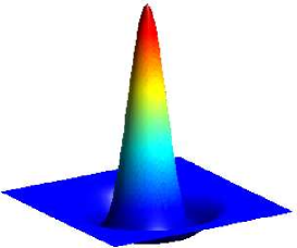
(a)

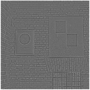
(b)

Figure 6: (a) The Marr wavelet (or Mexican hat). (b) Marr Wavelet singularity detector of the Haar-Riesz Memorial plaque.

In two dimensions, the most natural extension of the $1$-D-CWT is obtained by considering isotropic wavelets, i.e., wavelets $\psi\in\mathbb{L}^{2}(\mathbb{R}^{2})$ such that $\psi(\boldsymbol{x})=\psi_{\rm rad}(\|\boldsymbol{x}\|)$, with $\boldsymbol{x}=(x_{1},x_{2})$, for some radial function $\psi_{\rm rad}:\mathbb{R}_{+}\to\mathbb{R}$. In that case, the wavelet family is generated by $2$-D dilations and translations, i.e., we work with $\psi_{(\boldsymbol{b},a)}(\boldsymbol{x})={\textstyle\frac{1}{a}}\psi(\tfrac{\boldsymbol{x}-\boldsymbol{b}}{a})$ that are copies of $\psi$ translated to $\boldsymbol{b}=(b_{1},b_{2})\in\mathbb{R}^{2}$ and dilated by $a>0$. The $2$-D CWT of the image $f\in\mathbb{L}^{2}(\mathbb{R}^{2})$ is then simply $W_{f}(\boldsymbol{b},a)=\langle\psi_{(\boldsymbol{b},a)},f\rangle$ and the reconstruction of $f$ is guaranteed by

$$f(\boldsymbol{x})\ =\ \tfrac{2\pi}{c_{\psi}}\int_{0}^{+\infty}\!\!\!\int_{\mathbb{R}^{2}}\ W_{f}(\boldsymbol{b},a)\ \psi_{(\boldsymbol{b},a)}(\boldsymbol{x})\ {\rm d}^{2}\boldsymbol{b}\,\tfrac{{\rm d}a}{a^{3}},$$ (5)

if $c_{\psi}=(2\pi)^{2}\int_{\mathbb{R}^{2}}|\hat{\psi}(\boldsymbol{k})|^{2}/\|\boldsymbol{k}\|^{2}\ {\rm d}^{2}\boldsymbol{k}<\infty$. The isotropic CWT is a useful analysis tool for edge detection in images. For instance, by taking the (admissible) Marr Wavelet $\psi(\boldsymbol{x})=\Delta[\exp-{\textstyle\frac{1}{2}}\|\boldsymbol{x}\|^{2}]$ (with $\Delta$ the $2$-D Laplacian) also called Laplacian of Gaussian or Mexican Hat (see Fig. 6(a)), the CWT of an image $f$ acts as a multiscale edge detector. The topic of $1$-D and $2$-D continuous wavelet transforms is covered in more details in [52, 53, 54, 55, 33].

2.3 Discrete Scale-Space Representations

Numerical computation requires that continuous expansions such as (3) and (5) be discretized. In this section, we detail some parameter samplings, such as dyadic or translation invariant grids. Together with a suitable choice of the wavelet function, they lead to stable representations where the original signal can be perfectly reconstructed from its coefficients.

2.3.1 Multiresolution Analysis (MRA)

In the context of a dyadic sampling where $a=2^{j}$ and $b=n2^{j}$ for $j,n\in\mathbb{Z}$, the canonical way to design a suitable wavelet function $\psi$ in $1$-D makes use of a multi-resolution analysis (MRA). It is defined as a nested sequence of closed vector subspaces $\left(V_{j}\right)_{j\in\mathbb{Z}}$ in $\mathbb{L}^{2}(\mathbb{R})$ verifying standard properties [56]. Multiresolution analysis of a signal $f$ consists of successively projecting the signal onto subspaces $V_{j}$ in a series of increasingly coarser approximations as $j$ grows. The difference between two successive approximations represents detail information. It amounts to the information loss between two consecutive scales, which lies in the subspace $W_{j}$, the orthogonal complement of $V_{j}$ in $V_{j-1}$ such that:

$$V_{j-1}=V_{j}\oplus W_{j}.$$

Then, with additional stability properties, there exists a wavelet $\psi\in\mathbb{L}^{2}(\mathbb{R})$ such that $\mathcal{B}=\{2^{-j/2}\psi(2^{-j}x-n):n\in\mathbb{N}\}$ is an orthonormal basis for $W_{j}$.

2.3.2 Separable Orthogonal Wavelets

A $2$-D orthogonal wavelet basis $\mathcal{B}=\{\psi_{\boldsymbol{m}}\}_{\boldsymbol{m}}$ of $\mathbb{L}^{2}(\mathbb{R}^{2})$ for $\boldsymbol{m}=(j,\boldsymbol{n},k)$ is parameterized by a scale $2^{j}$ ($j\in\mathbb{Z}$), a translation $2^{j}\boldsymbol{n}=2^{j}(n_{1},n_{2})$ ($\boldsymbol{n}\in\mathbb{Z}^{2}$) and one of three possible orientations $k\in\{V,H,D\}$, loosely denoting the vertical, horizontal and (bi) diagonal directions, the latter being poorly representative. Wavelet atoms are defined by dyadic scalings and translations $\psi_{\boldsymbol{m}}(\boldsymbol{x})=2^{-j}\psi^{k}(2^{-j}\boldsymbol{x}-\boldsymbol{n})$ of three tensor-product $2$-D wavelets

$$\psi^{V}(\boldsymbol{x})=\psi(x_{1})\phi(x_{2}),\quad\psi^{H}(\boldsymbol{x})=\phi(x_{1})\psi(x_{2}),\quad\text{and}\quad\psi^{D}(\boldsymbol{x})=\psi(x_{1})\psi(x_{2}),$$

where $\phi$ and $\psi$ are respectively $1$-D orthogonal scaling and wavelet functions, see [54, 57, 33]. When the scale interval is limited to $j<J$ for some $J\in\mathbb{Z}$, the basis $\mathcal{B}$ is completed by the functional set $\mathcal{A}=\{\phi_{(J,\boldsymbol{n})}\}_{\boldsymbol{n}}$, with the $2$-D separable scaling function $\phi(\boldsymbol{x})=\phi(x_{1})\phi(x_{2})$. This set gathers all the coarse scale wavelet atoms with $j\geqslant J$. The standard cascade image is depicted in Fig. 7. It is now critically sampled, i.e., free from redundancy (compare Fig. 5 and 6(b)). The approximation coefficients in $\mathcal{A}$, a coarse image approximation at scale $J$, are represented in the bottom-left square of Fig. 7. The other squares in this picture, associated to the “bands” $\{V,H,D\}$ for $j<J$, exhibit some sparsity (few important coefficients), and horizontal and vertical edges are relatively well captured.

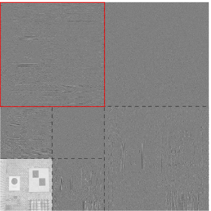
Figure 7: Dyadic wavelet decomposition of the Haar-Riesz Memorial plaque.

A non-linear approximation $f_{M}=H_{T}(f,\mathcal{B})$ in an orthogonal separable wavelet basis is efficient for smooth images or images with point-wise singularities. The approximation of a piecewise smooth image with edges of finite length decays like $\|f-f_{M}\|^{2}=O(M^{-1})$. This result extends to functions with bounded variations [58], and is asymptotically optimal. This decay is nevertheless not improved when the edges are smooth curves, because of the fixed ratio between the horizontal and the vertical sizes of the orthogonal wavelet support.

2.3.3 Fast Algorithms for Finite Images

A finite discretized image $f\in\mathbb{C}^{N_{1}\times N_{2}}$ of $N=N_{1}N_{2}$ pixels fits into the MRA framework by assuming that the pixel values of $f_{\boldsymbol{n}}$ on $\boldsymbol{n}=(n_{1},n_{2})$ are the coefficients $\langle\phi_{(J,\boldsymbol{n})},\tilde{f}\rangle$ of some continuous function $\tilde{f}\in\mathbb{L}^{2}(\mathbb{R}^{2})$ at a fixed resolution $V_{J}$, where $2^{2J}=N$.

The coefficients $\langle\psi_{j,\boldsymbol{n}}^{k},\,f\rangle$ of $\tilde{f}$ for $j\geqslant J$ are computed from the discrete image $f$ alone. This computation is performed using a cascade of filters interleaved with downsampling operators [56]. For compactly supported wavelets, this requires $O(N)$ operations. Symmetric bi-orthogonal wavelet bases with compact support ease the implementation of non-periodic boundary conditions [59]. For infinite impulse response (IIR) wavelet filters, computations in the Fourier domain require $O(N\log(N))$ operations [60], while recursive implementations [61] allow signal-adaptive implementation.

While separable wavelets are not optimal for approximating generic edges, they lie at the heart of early state-of-the-art methods for compression and denoising. The JPEG 2000 coding standard [62] performs an embedded quantization of wavelet coefficients, and uses an adaptive entropic coding scheme that takes into account the local dependencies across wavelet coefficients. The sub-optimality of wavelets for the sparse representation of edges can be alleviated using block thresholding of groups of wavelet coefficients [63], that gives improvements over scalar thresholding. Advanced statistical modeling of wavelet coefficients leads to denoising methods close to the state-of-the-art, see for instance [64, 65, 66].

2.3.4 Translation Invariant Wavelets

Given a discrete frame $\mathcal{B}=\{\psi_{\boldsymbol{m}}\}_{m}$ of $\mathbb{C}^{N}$, $\mathcal{B}$ is translation invariant if $\psi(\cdot-\tau)\in\mathcal{B}$ for any $\psi\in\mathcal{B}$ and any integer translation $\tau$. This property tends to reduce artifacts in image restoration problems like denoising, since, for such invariant frame, the thresholding operator $H_{T}(f,\mathcal{B})$ becomes itself translation invariant. Discrete orthogonal wavelet bases described in the previous sections are not translation invariant and many authors have worked on recovering this useful capability.

For instance, cycle spinning, proposed by Coifman and Donoho in [67], reduces wavelet artifacts by averaging the denoising result of all possible translates of the image, thus resulting in a translation invariant processing. For an orthogonal basis $\mathcal{B}=\{\psi_{\boldsymbol{m}}\}_{\boldsymbol{m}}$, this is equivalent to considering a tight frame which is the union of all translated bases $\{\psi_{\boldsymbol{m}}(\cdot-\tau)\}_{\boldsymbol{m},\tau}$. For a generic basis, this frame has up to $N^{2}$ atoms. For a wavelet basis, the frame has $O(N\log(N))$ atoms, and the coefficients are computed with the fast “à trous” algorithm in $O(N\log(N))$ [60, 68]. The translation invariant paradigm additionally draws a connection between the scale-space formalism (Sec. 2.1) [69] and thresholding (Sec. 1.3.2). Several $2$-D design described in the next sections attempt to (approximately) address invariance (translation/rotation) without sacrificing computational efficiency.

3 Oriented and Geometrical Multiscale Representations

The variety of oriented and geometric multiscale representations proposed over the last few years requires broad grouping, arranged as follows: Sec. 3.1 presents directional methods closely related to $1$-D decompositions. In Sec. 3.2, the directionality is addressed with diverse non-separable schemes. Finally, in Sec. 3.3, directionality is attained by an anisotropic scaling of the atoms that yields various efficient edge and curve representations.

3.1 Directional Outcrops from Separable Representations

3.1.1 Improved Separable Selectivity by Relaxing Constraints

As discussed in Sec. 2.3.1, discrete orthogonal wavelets may be viewed as a peculiar instance of orthogonal filter banks [70]. A well-known limitation in $1$-D is that orthogonality (hence non-redundant), realness, symmetry and finite support properties cannot coexist with pairs of low- and high-pass filters, except for the Haar wavelet.

We decide to briefly mention here some of the early steps taken to tackle this limitation. These have also been employed in more genuine non-separable transforms, as seen later, typically relaxing one of the aforementioned properties, such as using infinite-support filters [71], semi- or biorthogonal decompositions [59] or complex filter banks [72].

For instance, instead of a two-band filter bank, $M$-band wavelets [73] with $M>2$ provide alternatives where symmetry, orthogonality and realness are compatible with finitely supported atoms. In this setting, the approximation and the $M$-band detail spaces are $V_{j}$ and $(W^{m}_{j})_{m\in{\mathbb{N}}^{\star}_{M}}$ related through $V_{j-1}=V_{j}\oplus\bigoplus_{m=1}^{M-1}W^{m}_{j}$ for a resolution level $j$. This versatile design provides filters that suffer less aliasing artifacts with increased regularity. Their finer subband decomposition is also beneficial for detecting orientations in a more subtle fashion than with the $\{V,H,D\}$ quadrants obtained with standard wavelets (Sec. 2.3.2). Yet, more general $M$-adic MRAs are possible, for instance with a rational $M=p/q,M>1$ [74, 75, 76, 77, 78]. Note that for specific purposes such as compression, $M$-band filter banks with $M=2^{J},J\in\mathbb{N}$ may be treated like a $J$-level dyadic tree and combined in a hierarchical transform [79, 80]. Satisfying the MRA axioms is not necessary in practice in order to yield high performance results. This is suggested by recent image and video coders focusing on “simpler” transforms, closer to ancient Walsh-Hadamard transforms than to more involved wavelets [81].

Alternatively, the $1$-D decomposition on rows and columns of images may be performed in a more anisotropic manner, as in [82, 83]. An additional relaxation comes from lifting the critically sampled scheme, yielding oversampled, translation-invariant (see Sec. 4.2.3) multiscale wavelets, wavelet/cosine packets or frames [67, 84, 85, 86, 87, 88]. Multidimensional oversampled filter banks in n$-D$ with limited redundancy may be designed as well [89, 90, 91, 92, 93].

3.1.2 Pyramid-related wavelets

Notably influenced by [94, 95], Unser and Van de Ville propose a slightly redundant transform [96] based on a pyramid-like wavelet analysis. This decomposition constitutes a wavelet frame with mild redundancy, which is nevertheless not steerable. Subsequently, the same authors propose a steerable analysis [97] based on polyharmonic $B$-splines [98] and the Maar-like [5, 99] wavelet pyramid. Such multiresolution analysis can easily be implemented via filter banks as detailed in [97] and the total redundancy of this decomposition is $8/3$ (a redundancy of $4/3$ is introduced by the pyramid structure and the complex nature of the coefficients increases the redundancy by a factor of $2$). A similar approach based on Riesz-Laplace wavelets is proposed in [100]. The latter constructions are related to Hilbert and Riesz transforms.

3.1.3 Complexifying Discrete Wavelets with Hilbert and Riesz

Different kinds of complexification are indeed a possible option in order to tackle the problem of poor directionality with classical wavelet transforms. The common basic idea leans toward analytic wavelets and their combination to improve the $2$-D directionality. Behind a generic notion of complex wavelets reside different approaches detailed hereafter, which require the definition of some basic tools.

We first introduce the Hilbert transform, termed “complex signal” in [101] and exhaustively mapped in [102]. While the $1$-D Hilbert transform is unambiguously defined, there exists multidimensional extensions, often obtained by tensor products, thus leading to approximations. In order to increase the directionality property, other multidimensional constructions (discussed in [103]) have also been proposed.

• The $1$-D Hilbert transform $\mathcal{H}$ of a signal $f$ is easily expressed in the Fourier domain as

  $$\mathcal{H}\{f\}(\omega)=-{\rm i}\operatorname{sign}(\omega)\widehat{f}(\omega).$$ (6)

• The $1$-D fractional Hilbert transform $\mathcal{H}_{\theta}$ of $f$ is similarly defined in [104] by

  $$\mathcal{H}_{\theta}\{f\}(\omega)=\exp({\rm i}\pi\theta\operatorname{sign}(\omega))\widehat{f}(\omega).$$ (7)

• The $2$-D directional Hilbert transform $\mathcal{H}_{\theta}$ of $f$ is one of the $2$-D extensions defined in [104] as

  $$\mathcal{H}_{\theta}\{f\}(\omega_{1},\omega_{2})=-{\rm i}\operatorname{sign}\big{(}\cos(\theta)\omega_{1}+\sin(\theta)\omega_{2}\big{)}\widehat{f}(\omega_{1},\omega_{2}).$$ (8)

  See also [105].

The Hilbert transform was already associated with wavelets for transient detection by Abry et al. [106]. Others early connections between wavelets and the Hilbert transform are drawn in [107, 108, 109]. At the end of the 1990’s, Kingsbury proposed the dual-tree transform based on even and odd filters [110, 111]. An alternative construction is given by Selesnick [112]. It amounts to performing two discrete classical wavelet transforms in parallel, the wavelets generated by the trees forming Hilbert pairs. An atom of the corresponding basis (here the diagonal wavelet) and its corresponding frequency plane tiling are depicted in Fig. 9. The corresponding dual-tree of wavelet coefficients is represented in Fig. 8, which clearly shows the separation of oriented structures with different orientations. The resulting oriented wavelet dictionary has a small redundancy and is also computationally efficient. The corresponding wavelet is approximately shift invariant, see [113] for more details. It is extended to the $M$-band setting by Chaux et al. [114] and to wavelet packets in [115, 116]. In Fig. 10, one subband of the wavelet transform (red square in Fig. 7), two subbands (primal+dual) of the dyadic dual-tree transform (red squares in Fig. 8), as well as the corresponding eight subbands (4 primal+4 dual) of the $4$-band dual-tree wavelet decomposition are depicted. In Fig. 10(c), the fine oriented textures from the left side of the image are (slightly) better separated in some non-horizontal subbands. The wavelet/frequency tiling corresponding to the $4$-band dual-tree wavelet decomposition are depicted in Fig. 11. The main advantage of this decomposition is that it achieves a directional image analysis with a small redundancy of a factor $2$ ($4$ for the complex transform).

Gopinath [117, 118] has designed phaselets which is an extension of the dyadic dual-tree wavelet transform [110, 119]. They aim at improving translation invariance with a given redundancy, and are built by carefully observing the effects of shifts in a discrete wavelet transform. $2$-D phaselets are easily obtained by tensor products.

More recently, the shiftability of the dual-tree transform has been studied by Chaudhury et al. [104] by introducing the fractional Hilbert transform (7). A $2$-D extension has been proposed in [120] and the construction of Hilbert transform pairs of wavelet bases can be found in [121]. Note that previous works dealing with multidimensional extensions have been first reported for instance in [122] and then in [123, 124] using the notion of hypercomplex wavelets.

Numerous extension to multidimensional signals have been proposed, see for instance [125, 126]. They, for instance, use the Riesz transform $\mathcal{R}$, which is defined in the frequency domain as follows:

$$\widehat{\mathcal{R}}\{f\}=(\widehat{\mathcal{R}}_{1}\{f\},\dots,\widehat{\mathcal{R}}_{N}\{f\}).$$ (9)

where

$$\forall n\in\{1,\,\cdots,N\},\qquad\widehat{\mathcal{R}}_{n}\{f\}(\boldsymbol{\omega})=-{\rm i}\frac{\omega_{n}}{\|\boldsymbol{\omega}\|}\widehat{f}(\boldsymbol{\omega}).$$ (10)

Other recent extensions of multidimensional oriented wavelets are based on the notion of monogenic signal/wavelet [127, 128, 129]. We finally mention that other methods have been developed in order to achieve directional analytic wavelets such as softy space projections [130, 131, 132, 133, 134] or the Daubechies complex wavelets [135, 136, 137]. Complex wavelets have also been shown to provide robust image similarity measures [138, 139].

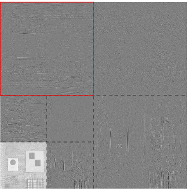
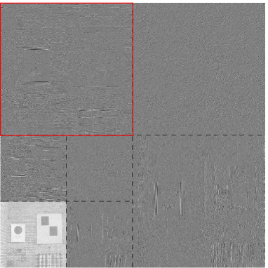
Figure 8: Dyadic dual-tree wavelet decomposition of the Haar-Riesz Memorial plaque.

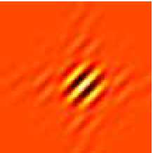
(a)

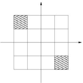
(b)

Figure 9: The dyadic dual-tree wavelet. (a) Example of atom (diagonal wavelet). (b) Associated frequency partitioning.

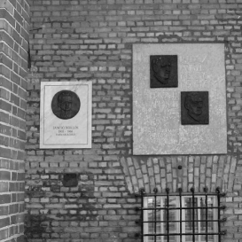
(b)

(a)

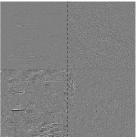
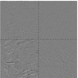
(c)

Figure 10: The original image (a) and the horizontal subband(s) at first resolution level for (b) Dyadic wavelet transform, (c) Dyadic dual-tree transform (primal+dual) and (d) $M$-band dual-tree wavelet decomposition (primal+dual) of the Haar-Riesz Memorial plaque.

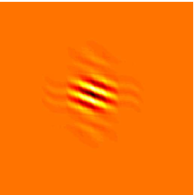
(a)

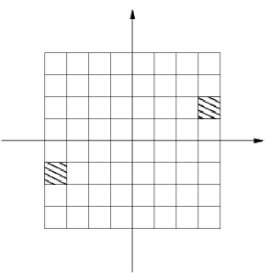
(b)

Figure 11: The $M$-band dual-tree wavelet. (a) Example of atom. (b) Frequency partinioning.

3.2 Non-Separable Directionality

3.2.1 Non-separable Decomposition Schemes

In contrast to the separable constructions detailed in Sec. 3.1.1 where $n$-D representations are composed of $1$-D transforms applied separately along each dimension (sometimes recombined, as in the dual-tree wavelet case or in [140]), non-separable constructions are directly performed in $n$-D. Since the literature on this topic is large, this section is focussed on a limited number of references dealing with directional multiscale decompositions.

These works are often related to non-diagonal subsampling operators, non-rectangular lattices (e.g., quincunx grids or integer lattices) [141, 142], or non-separable $n$-D windows [143, 144]. Complementary standard references can be found in [70, p. 558 sq.] or [145, 146, 147]. Some of these constructions are defined using the lifting scheme, see Sec. 4.3 and 5.3 for more details. While directional filter banks do not provide a multiscale representation in general, $2$-band [148, 149, 150] or even $M$-band non-redundant directional discrete wavelets [151] have been proposed. Non-separable schemes are used for instance as building blocks for multiscale geometric decompositions such as:

• directional filter banks in [152], and their combination with a Laplacian pyramid in contourlets [153, 154] or surfacelets [155],

• (pseudo-) polar fast Fourier transform (FFT) [156] in first generation curvelets described in Sec. 3.3.2, or the loglets in [157] that exhibit a polar separability.

In order to overcome the limited efficiency of the standard $2$-D separable DWT for representing non-horizontally or vertically directed edges (see Sec. 2.3.2), several authors have adapted $1$-D concepts for local edge representation. Reissell [158] develops, for instance, a pseudo-coiflet scheme that addresses numerically efficient interpolation for a parametric wavelet representation of curves. Moreover, for digital images it would be beneficial to follow contours on more appropriate discrete paths (see [159] for an early application) such as discrete lines [160, 161, 162]. While discrete lines are adapted to digital ridgelets in [163], Velisavljević et al. propose multidirectional anisotropic directionlets [164], based on skewed lattices, with directional vanishing moments along direction with rational slopes, still relying on a simple separable implementation. This approach is refined in [165] by taking lifting steps of $1$-D wavelets along an explicit orientation map defined on a quincunx multiresolution sampling grid, and in [166] with a more efficient representation for sharp features. A combination of $2$-D filter banks and $1$-D directional filter bank is devised in [167, 168]. Similar ideas have been recently applied to edge detection in [169]. In [170], non-adaptive directional wavelet frames are constructed with Haar wavelets and a finite collection of “shear” matrices. Krommweh also proposes tetrolets, an adaptive variation (akin to digital wedgelets) of Haar-like wavelets on compact tetrominoes (geometric shapes composed of four squares, connected orthogonally, see [171]). These last constructions may further sparkle the growing interest of the association of multiscale analysis and discrete geometry [172].

3.2.2 Steerable Filters

Steerable filters [173, 174, 175] were developed in order to achieve more precise feature detectors adapted to image edge junctions (often termed “X”, “T” and “L” junctions). Their construction allows one to compute multiscale derivatives at any orientation (steerability) from a linear combination of a small number of fixed filters. In [174], the construction starts from a bidimensional Gaussian $G(\boldsymbol{x})=\exp(-\frac{1}{2}\|\boldsymbol{x}\|^{2})$ for $\boldsymbol{x}=(x_{1},x_{2})$ with associated base (differential) filters ${\mathcal{G}}^{0}(\boldsymbol{x})=\tfrac{\partial}{\partial x_{1}}G(\boldsymbol{x})$ and ${\mathcal{G}}^{\pi/2}(\boldsymbol{x})=\tfrac{\partial}{\partial x_{2}}G(\boldsymbol{x})$.

From the properties of the directional derivative, filters “steered” at angle $\theta\in[0,2\pi)$ are then built from

$${\mathcal{G}}^{\theta}(\boldsymbol{x})\ =\ \cos(\theta)\,{\mathcal{G}}^{0}(\boldsymbol{x})\ +\ \sin(\theta)\,{\mathcal{G}}^{\pi/2}(\boldsymbol{x}).$$ (11)

where $\cos(\theta)$ and $\sin(\theta)$ may be interpreted as interpolators. Since the convolution is linear, the resulting steered decomposition arises from a combination of images that underwent ${\mathcal{G}}^{0}$ or ${\mathcal{G}}^{\pi/2}$ filters. A larger class of asymmetric oriented filters is proposed in [176]. Their angular parts are derived from even and odd functions:

$$\forall\varphi\in[0,2\pi),\qquad h_{e}(\varphi)=\sum_{n=1}^{N}w_{n}\cos(n\varphi)\qquad\mbox{and}\qquad h_{o}(\varphi)=\sum_{n=1}^{N}w_{n}\sin(n\varphi),$$ (12)

which form Hilbert transform pairs (see Sec. 3.1.3), unlike the resulting spatial filters. An angle $\theta$ rotation is obtained through:

$$h_{e}(\varphi-\theta)=\boldsymbol{k}_{e}(\theta)^{T}\boldsymbol{f}(\varphi)\qquad\mbox{and}\qquad h_{o}(\varphi-\theta)=\boldsymbol{k}_{o}(\theta)^{T}\boldsymbol{f}(\varphi),$$ (13)

where $\boldsymbol{k}_{e}(\theta)$ and $\boldsymbol{k}_{o}(\theta)$ are interpolating vectors and $\boldsymbol{f}(\varphi)$ is a weighted Fourier vector, namely:

$$\boldsymbol{k}_{e}(\theta) =\big{[}\,\phantom{-}\cos\theta,\sin\theta,\phantom{-}\cos(2\theta),\sin(2\theta),\ \cdots\ ,\phantom{-}\cos(N\theta),\sin(N\theta)\big{]}^{T},$$

$$\boldsymbol{k}_{o}(\theta) =\big{[}-\sin\theta,\cos\theta,-\sin(2\theta),\cos(2\theta),\ \cdots\ ,-\sin(N\theta),\cos(N\theta)\big{]}^{T},$$

$$\boldsymbol{f}(\varphi) =\big{[}\,w_{1}\cos\varphi,w_{1}\sin\varphi,w_{2}\cos(2\varphi),w_{2}\sin(2\varphi),\cdots,w_{N}\cos(N\varphi),w_{N}\sin(N\varphi)\big{]}^{T}\!\!.$$

If we set $\theta=\theta_{n}=2\pi n/N$ for $1\leqslant n\leqslant N$, filters $h_{e}(\cdot-\theta)$ and $h_{o}(\cdot-\theta)$ may be rewritten as a linear combination of $h_{e}(\cdot-\theta_{n})$ and $h_{o}(\cdot-\theta_{n}),\,1\leqslant n\leqslant N$. An example of decomposition with four orientations and two scales is represented in Fig. 12, with corresponding projection atoms in Fig. 13. Steerable filters may be combined with discrete wavelets to improve their radial properties [177, 178].

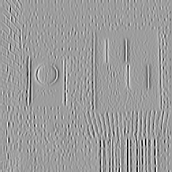
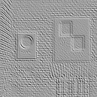
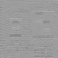
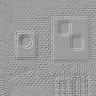
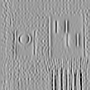
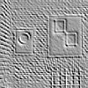
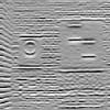
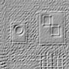
Figure 12: Steerable pyramid decomposition of the Haar-Riesz Memorial plaque, over two scales, with four orientations.

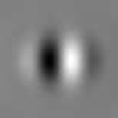
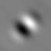
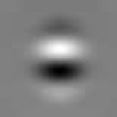
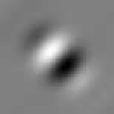
Figure 13: Example of steerable pyramid atoms with four orientations.

3.2.3 Directional Wavelets and Frames

In Sec. 2.2, the two-dimensional Continuous Wavelet Transform ($2$-D CWT) was defined as a straightforward extension of the $1$-D CWT using isotropic wavelets. It is however possible to make use of more complicated group actions to drive the CWT parameterization in the plane, such as rotations or the similitude group SIM$(2)$, see [147].

Consequently, given a mother function $\psi\in\mathbb{L}^{2}(\mathbb{R}^{2})$ that is well localized and oriented, we write

$$\psi_{(\boldsymbol{b},a,\theta)}(\boldsymbol{x})\ =\ {\textstyle\frac{1}{a}}\,\psi({\textstyle\frac{1}{a}}\,R_{\theta}^{-1}\big{(}\boldsymbol{x}-\boldsymbol{b})\big{)},$$

where $R_{\theta}$ stands for the $2\times 2$ rotation matrix. For a function $f\in\mathbb{L}^{2}(\mathbb{R}^{2})$, the 2-D CWT (non-isotropic) is thus

$$W_{f}(\boldsymbol{b},a,\theta)\ =\ \langle\psi_{(\boldsymbol{b},a,\theta)},f\rangle.$$

If the wavelet is admissible, i.e., if $c_{\psi}=(2\pi)^{2}\int_{\mathbb{R}^{2}}|\hat{\psi}(\boldsymbol{\omega})|^{2}/\|\boldsymbol{\omega}\|^{2}\ {\rm d}^{2}\boldsymbol{\omega}<\infty$, then, the CWT may be inverted through

$$f(\boldsymbol{x})\ =\ c^{-1}_{\psi}\int_{0}^{\infty}\!\!\!\tfrac{{\rm d}a}{a^{3}}\int_{0}^{2\pi}\!\!\!{\rm d}\theta\int_{\mathbb{R}^{2}}\!\!\!{\rm d}^{2}\boldsymbol{b}\quad W_{f}(\boldsymbol{b},a,\theta)\ \psi_{(\boldsymbol{b},a,\theta)}(\boldsymbol{x}),$$

the equality being valid almost everywhere on $\mathbb{R}^{2}$.

The selectivity power of the wavelet, that is, its ability to distinguish two close orientations in an image, may be measured in the Fourier domain. Typically, a good directional wavelet is thus a function whose Fourier transform is essentially or exactly contained in a cone with apex on the origin: the narrower the cone, the more selective the wavelet transform using that wavelet [147].

Practically, it is not satisfactory to manipulate a continuum of wavelets parameterized by continuous parameters. The question is therefore to know if it is possible to decompose and reconstruct an image from a discretized set of parameters, i.e., on the family $\mathcal{G}=\{\psi_{(\boldsymbol{b},a,\theta)}:\boldsymbol{b}\in\mathcal{P},a\in\mathcal{A},\theta\in\Theta\}$ with $\mathcal{P}\subset\mathbb{R}^{2}$, $\mathcal{A}\subset\mathbb{R}^{*}_{+}$ and $\theta\subset[0,2\pi)$ all discrete (countable) sets. As explained in Sec. 1.3.2, this question amounts to ask when $\mathcal{G}$ is a frame of $\mathbb{L}^{2}(\mathbb{R}^{2})$.

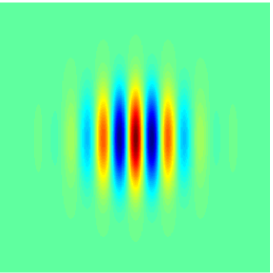
(a)

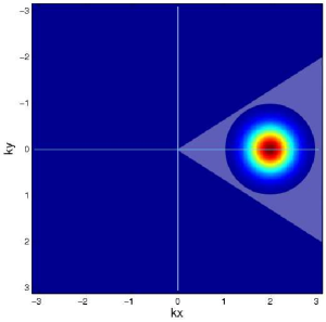
(b)

Figure 14: The Morlet Wavelet. (a) Spatial representation (real part). (b) Fourier representation. Supporting cone and frequency axes are drawn for illustration.

Such frames have been built for the Morlet (or Gabor) wavelet [179, 180]:

$$\psi(\boldsymbol{x})=G_{\sigma_{0}}(\boldsymbol{x})\ e^{{\rm i}\boldsymbol{\omega}_{0}\cdot\boldsymbol{x}}=e^{-\|\boldsymbol{x}\|^{2}/2\sigma_{0}^{2}}\ e^{{\rm i}\boldsymbol{\omega}_{0}\,\boldsymbol{x}},\quad\hat{\psi}(\boldsymbol{\omega})\propto G_{1/\sigma_{0}}(\boldsymbol{\omega}-\boldsymbol{\omega}_{0})=e^{-\sigma_{0}^{2}\|\boldsymbol{\omega}-\boldsymbol{\omega}_{0}\|^{2}/2},$$

where $\boldsymbol{\omega}_{0}\in\mathbb{R}^{2}$ defines the cone axis and $\sigma_{0}>0$ is related to the cone aperture, as represented in Fig. 14. Notice that approximate quadrature filters exist to accelerate the computation of the wavelet coefficients [181]. The Conic (or Cauchy) wavelet, whose spectral support is exactly contained into a cone, can also be used in order to define a frame [105].

Finally, a multiresolution structure can also be put on the angular dependency of the conic wavelets in the frequency domain to define multiselective wavelets [182]. This generates a redundant basis that may represent jointly a large spectrum of features ranging from highly directional ones (e.g., edges) to isotropic elements (e.g., spots, corners) and including intermediate directional structures such as textures.

3.3 Directionality in Anisotropic Scaling

3.3.1 Ridgelets

Ridgelets [183, 184] and wavelet X-ray transforms [185] appear as a combination of a $1$-D wavelet transform and the Radon transform [186]. They are designed for efficient representation of discontinuities over straight lines. A bivariate ridgelet transform is constant along parameterized lines $x_{1}\cos(\theta)+x_{2}\sin(\theta)=b$ and defined for $a>0$, $b\in\mathbb{R}$ and $\theta\in[0,2\pi)$, by

$$\forall{\boldsymbol{x}}=(x_{1},x_{2})\in\mathbb{R}^{2},\qquad\psi_{(\boldsymbol{b},a,\theta)}({\boldsymbol{x}})=a^{-1/2}\,\psi((x_{1}\cos(\theta)+x_{2}\sin(\theta)-b)/a).$$ (14)

Ridgelet coefficients for the image $f$ are given by

$$\mathcal{R}_{f}(b,a,\theta) =\int\psi_{(\boldsymbol{b},a,\theta)}({\boldsymbol{x}})\,f({\boldsymbol{x}})\,{\rm d}^{2}{\boldsymbol{x}}$$

$$=\int\mathfrak{R}_{f}(\theta,t)\,a^{-1/2}\psi((t-b)/a)\,{\rm d}t,$$ (15)

where $\mathfrak{R}_{f}(\theta,t)$ represents the Radon transform of $f$ defined by:

$$\mathfrak{R}_{f}(\theta,t)=\int\int f(x_{1},x_{2})\,\delta(x_{1}\cos(\theta)+x_{2}\sin(\theta)-t)\,{\rm d}x_{1}{\rm d}x_{2},$$ (16)

with $\delta$ denoting the Dirac distribution. The ridgelet transform may be interpreted as a $1$-D wavelet transform of Radon slices where the angle $\theta$ is constant and $t$ varies. Several implementations and variations exist in order to overcome the issues raised by the Radon transform discretization, such as the finite ridgelet transform [187], the approximate digital ridgelet transform [188] or the discrete analytical ridgelet transform [189]. Their multiscale implementation [16] is the basis for the first generation curvelets described in Sec. 3.3.2. A ridgelet decomposition [190] of the Haar-Riesz Memorial plaque is given in Fig. 15, with a typical atom along with a synthetic description of its implementation in Fig. 16.

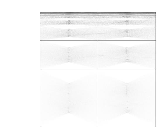
Figure 15: Ridgelet decomposition (square root scale) of the Haar-Riesz Memorial plaque.

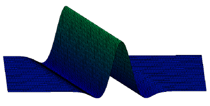
(a)

(b)

Figure 16: The Ridgelet transform. (a) Example of atoms. (b) Synthetic implementation description.

3.3.2 Curvelets

The curvelet representation, introduced by Candès and Donoho [16, 191], improves the approximation of cartoon images with $\text{C}^{2}$ edges with respect to wavelets. We review here the second generation of curvelets, as introduced in [191].

Continuous Curvelet Transform

A curvelet atom, with scale $s$, orientation $\theta\in[0,\pi)$, position ${\boldsymbol{y}}\in[0,1]^{2}$ is defined as

$$\psi_{s,{\boldsymbol{y}},\theta}({\boldsymbol{x}})=\psi_{s}(R_{\theta}^{-1}({\boldsymbol{x}}-{\boldsymbol{y}}))$$ (17)

where $\psi_{s}({\boldsymbol{x}})\approx s^{-3/4}\,\psi(s^{-1/2}x_{1},s^{-1}x_{2})$ is approximately a parabolic stretch of a curvelet function $\psi$ with vanishing moments in the vertical direction. At scale $s$, a curvelet atom is thus a needle oriented in the direction $\theta$ whose envelope is a specified ridge of effective length $s^{1/2}$ and width $s$, and which displays an oscillatory behavior transverse to the ridge.

A curvelet atom thus benefits from a parabolic scaling property $width=length^{2}$ that is a major departure from oriented wavelets. Fig. 17 presents an example of a curvelet atom, together with its Fourier transform, for the second generation of curvelets. The resulting curvelet Fourier tiling resembles that of the Cortex transform [192].

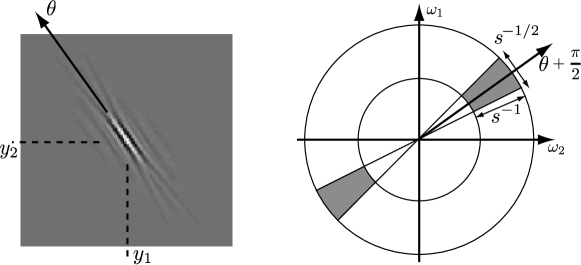
Figure 17: Left: Example of a curvelet $\psi({\boldsymbol{x}},s,{\boldsymbol{y}},\theta)$. Right: the frequency support of $\hat{\psi}(\omega,s,{\boldsymbol{y}},\theta)$ is a wedge.

The continuous curvelet transform computes the set of inner products $\langle\psi_{s,{\boldsymbol{y}},\theta}(\cdot),\,f\rangle$ for all possible $(s,{\boldsymbol{y}},\theta)$. A careful design of $\psi_{s}$ [191] enables a conservation of energy and a simple reconstruction formula. The decay of the curvelet transform as $s$ decreases allows one to detect the position and orientation of contours [193].

Curvelet Frame

The continuous curvelet representation is sampled in order to obtain a curvelet frame $\mathcal{B}=\{\psi_{\boldsymbol{m}}\}_{\boldsymbol{m}}$, [191], see also [194] for the description of a complex curvelet tight frame.

A curvelet atom, with scale $2^{j}$, orientation $\theta_{\ell}\in[0,\pi)$, position ${\boldsymbol{x}}_{n}\in[0,1]^{2}$ is defined from the continuous atom (17)

$$\psi_{\boldsymbol{m}}({\boldsymbol{x}})=\psi_{2^{j},\theta_{\ell},{\boldsymbol{x}}_{n}}({\boldsymbol{x}})\quad\text{where}\quad m=(j,n,\ell)$$

where the sampling locations are

$$\theta_{\ell}=\ell\pi 2^{\lfloor j/2\rfloor-1}\in[0,\pi)\quad\text{and}\quad{\boldsymbol{x}}_{n}=R_{\theta_{\ell}}(2^{j/2}n_{1},2^{j}n_{2})\in[0,1]^{2}.$$

The curvelet parameters are sampled using an increasing number of orientations at finer scales. This sampling is the key ingredient to ensure the tight frame property [191], which provides a simple reconstruction formula.

A fast discrete curvelet transform computes the set of inner products $\{\langle\psi_{\boldsymbol{m}},\,f\rangle\}_{\boldsymbol{m}}$ in $O(N\log(N))$ operations for an image with $N$ pixels, see [195]. The coronae and rotations of the continuous settings are replaced by their discrete Cartesian counterparts, i.e. concentric squares and shears. Figure 18 shows an example of curvelets decomposition.

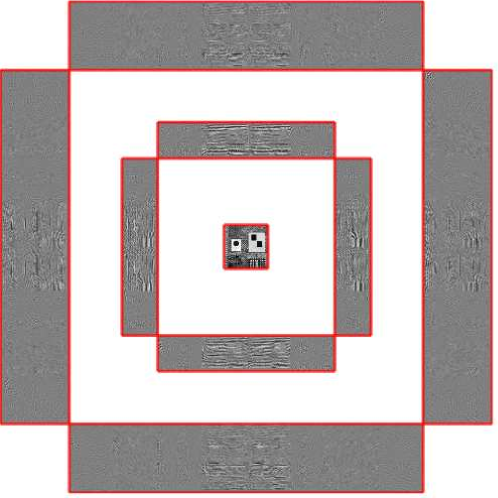
Figure 18: Curvelet decomposition of the Haar-Riesz Memorial plaque. The layout of the coefficients follows the frequency localization of curvelet atoms.

Candès and Donoho prove [196] that the curvelet non-linear approximation $f_{M}=H_{T}(f,\mathcal{B})$, where $H_{T}$ is defined in (2), ensures an approximation error decay $\|f-f_{M}\|^{2}=O(M^{-2}\log^{3}(M))$ for a $\text{C}^{2}$ regular image outside $\text{C}^{2}$ regular edge curves. This is a significant improvement over the $O(M^{-1})$ error decay of a wavelet approximation described in Sec. 2.3.2, and is achieved with a fast $O(N\log(N))$ algorithm for discrete images. This asymptotic error decay is optimal (up to logarithmic factor) for the class of images that are $\text{C}^{2}$ regular outside $\text{C}^{2}$ regular edge curves, see [196]. Monogenic curvelets are proposed in [197] to obtain additional advantages over monogenic wavelets, described in Section 3.1.3.

Shearlet atoms [198, 199] are built similarly to curvelets, but they replace, in their continuous formulation, rotation and anisotropic stretch with anisotropic shears. The discrete shearlet transform [200, 201] is thus implemented similarly to the discret curvelet transform [195] using discrete shears. It provides the same approximation properties as curvelets, albeit with a different directional sensitivity (e.g., the number of orientations doubles at each scale). Recently a type-I ripplet transform [202] has been proposed as an extension to curvelets with alternative scaling laws.

3.3.3 Contourlets

Contourlets [153] are sometimes considered a low-redundancy discrete approximation of curvelets. Actually, they are designed in the spatial domain (instead of the frequency plane), aiming at a close-to-critical directional representation. Their construction is based on a Laplacian Pyramid [43] (see Fig. 5). The low-pass part of the pyramid is further decomposed with a biorthogoal 9/7 DWT. Each difference image obtained from the pyramid is subject to directional filter bank (see Sec. 3.2) (initially from [141], [203] proposes a simpler implementation based only on a quincunx structure). A contourlet decomposition is illustrated in Fig. 19. The resulting frequency plane tiling is represented in Fig. 20(c). The contourlet inherits its redundancy of $4/3$ from the pyramidal scheme. Its approximation rate is similar to that of curvelets (Sec. 3.3.2). At one end of the redundancy spectrum, [204] proposes a critically sampled version. At the other end, the constraints thus laid on the basis functions (Figs. 20(a)-20(b)) are relaxed by the design of a more redundant [154] version, based on non-subsampled (Sec. 3.1.1 )pyramid and directional filters.

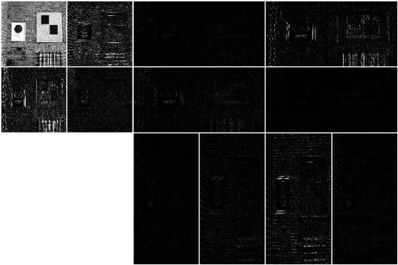
Figure 19: Contourlet decomposition of the Haar-Riesz Memorial plaque.

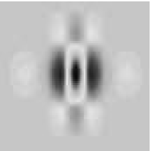
(a)

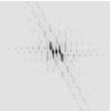
(b)

(c)

Figure 20: The contourlet transform. (a)-(b) Two typical atoms; (c) Frequency tiling.

3.3.4 Frames for Oscillating Textures.

While curvelets, contourlets and shearlets are optimized for the processing of edges, they are not tailored for the processing of oscillating textures, because of their poor frequency localization. Generic oscillating patterns can be captured using a local Fourier analysis on a regular segmentation of the image in squares. This corresponds to an expansion in a Gabor frame, see for instance [33]. The spatial segmentation can be optimized using a decomposition in a best cosine packet dictionary as described in Section 4.2.

Wavelet packets, detailed in Section 4.2, have been used to process and compress oscillating textures such as fingerprints. Brushlets [205], introduced by Meyer and Coifman, improve the frequency localization of wavelet packets.

Wave atoms [206] better capture geometric textures using an anisotropic scaling. The wavelength of wave-atom oscillations is proportional to the square of their diameter. This scaling allows a thresholding in a wave atom frame to optimally approximate textures obtained by a smooth warping of a sinusoidal profile, see [206].

4 Redundancy and Adaptivity

Highly redundant representations allow us to improve the representation of complicated images with edges and textures. However, as described hereafter, computing efficient image representations in such dictionaries sometimes requires approximations.

4.1 Pursuits in Redundant Dictionaries

An approximation $f_{M}$ of an image $f$ with $M$ atoms from a highly redundant dictionary $\mathcal{B}=\{\psi_{\boldsymbol{m}_{j}}:1\leqslant j\leqslant P\}$ is written

$$f_{M}=\Psi a=\sum_{j}\ a_{j}\,\psi_{\boldsymbol{m}_{j}},\quad\text{with}\quad\|a\|_{0}=\#\left\{j\,:\;a_{j}\neq 0\right\}\leqslant M.$$

Computing the $M$-sparse coefficients $a$ that produce the smallest error $\|f-f_{M}\|$ in a generic dictionary is NP-hard [207]. Furthermore, the $M$-terms approximation $f_{M}=H_{T}(f,\mathcal{B})$ computed by thresholding (2) might be quite far from the best $M$-terms approximation. One thus has to use approximate schemes in order to compute an efficient approximation in a reasonable time.

4.1.1 Matching Pursuits

Matching pursuit [208] computes $f_{M}$ from $f_{M-1}$ by choosing the atom $\psi_{\boldsymbol{m}}$ that minimizes the correlation $|\langle\psi_{\boldsymbol{m}},\,f-f_{M-1}\rangle|$. Orthogonal matching pursuit [33, 209] further reduces the approximation error by projecting $f$ on the $M$ chosen atoms to compute $f_{M}$.

Under restrictive conditions on the dictionary $\mathcal{B}$, these greedy algorithms compute an approximation $f_{M}$ that is close to the best $M$-term approximation, see for instance [210, 211]. These conditions typically require the correlation $|\langle\psi_{\boldsymbol{m}},\,\psi_{\boldsymbol{m}^{\prime}}\rangle|$ to be small for $\boldsymbol{m}\neq\boldsymbol{m}^{\prime}$, which is not applicable to highly redundant dictionaries typically used in image processing.

4.1.2 Basis Pursuit

A sparse approximation is obtained by convexifying the $\ell^{0}_{N}$ pseudo norm, and solving the following basis pursuit denoising convex problem [212]

$$f_{M}=\Psi a=\sum_{j}a_{j}\psi_{\boldsymbol{m}_{j}}\quad\text{where}\quad a\in\underset{\tilde{a}\,\in\,\mathbb{R}^{P}}{\operatorname{argmin}}\;{\textstyle\frac{1}{2}}\|f-\sum_{j}\tilde{a}_{j}\psi_{\boldsymbol{m}_{j}}\|^{2}+\mu\|\tilde{a}\|_{1},$$ (18)

where $\mu>0$ is adapted so that $\|a\|_{0}=M$. This problem (18) is minimized, for instance, using iterative thresholding methods [213, 214]. Algorithmic solutions to its generalized form as sums of convex functions (a common formulation to many data processing problems) may be solved with great flexibility in the framework of proximity operators [215].

Similarly to matching pursuit algorithms, this $\ell^{1}_{N}$ approximation can be shown to be close to the best $M$-term approximation if the atoms of $\mathcal{B}$ are not too correlated, see for instance [216, 211].

4.1.3 Pursuits in Parametric Dictionaries

Parametric dictionaries are obtained from basic operations (like rotation, translation, dilation, shearing, modulation, etc.) applied to a continuous mother function. Even if such dictionaries also define redundant bases similar to those introduced earlier, they deserve a separate description since their parametric nature provides them with some particular properties. They are generally created to provide a very rich and dense family of functions built from the geometrical features of the analyzed image. They have applications in image and video coding [217], multi-modal signal analysis (e.g., video plus audio) [218], and also for signal decomposition on non-Euclidean spaces [219].

Formally, given a set of $S$ transformations $T^{i}_{m_{i}}$ for $1\leqslant i\leqslant S$ parameterized by $m_{i}\in\Lambda_{i}\subset\mathbb{R}^{n_{i}}$, the parametric dictionary is related to a certain discretization of $\Lambda^{{\rm d}}\subset\Lambda=\Lambda_{1}\times\cdots\times\Lambda_{S}$, i.e.,

$$\mathcal{B}\ =\ \{\psi_{\boldsymbol{m}}({\boldsymbol{x}})=[T^{1}_{m_{1}}\cdots T^{S}_{m_{S}}\psi]({\boldsymbol{x}})\in\mathbb{L}^{2}(\mathbb{R}^{2}):\ \boldsymbol{m}=(m_{1},\cdots,m_{S})\in\Lambda^{{\rm d}}\}.$$

The directional wavelets described in Sec. 3.2.3 and the subsequent frames built from them are actually an example of parametric dictionaries with the translations $T^{1}_{m_{1}}T^{2}_{m_{2}}=T^{1}_{b_{1}}T^{2}_{b_{2}}$, the rotation $T^{3}_{m_{3}}=R_{\theta}$ and the dilation $T^{4}_{m_{4}}=D_{a}$ operations. For these wavelets, the decomposition/reconstruction methods are relatively easy to formulate, due to the continuous inversion formula or using the frame condition.

However, checking the frame condition may sometimes become tedious. In addition, more transformations of the mother function may be added in order to enlarge the family of functions, further worsening the frame bounds.

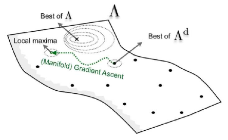
Figure 21: Explanation of the optimization in $\Lambda$ starting from a point in $\Lambda^{\rm d}$.

Fortunately, as described in Sec. 4.1 it is still possible to find good description of images in very general family of functions. Most of the time, since the Parametric Dictionaries are much larger than other dictionaries of controlled redundancy, the (Orthogonal) Matching Pursuit decomposition (Sec. 4.1.1) is used to find a sparse representation of signals.

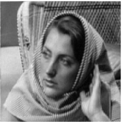
(a)

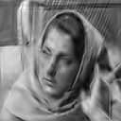
(b)

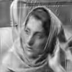
(c)

Figure 22: (a) Original image. (b) Reconstruction with 300 atoms for a rich parametric dictionary containing $5\times 5$ anisotropic scales, 8 orientations, and $N$ translations. PSNR : $26.63$ dB (CT: 4634s). (c) Optimized Reconstruction at 300 atoms starting from a dictionary with only $3\times 3$ scales, 4 directions and $N$ translations, PSNR : $26.68$ dB (CT: 949s).

Interestingly, thanks to the parametric nature of $\mathcal{B}$, the dictionary discretization can be refined during the Matching Pursuit iterations. Indeed, since $\mathcal{B}$ is the discretization of the continuous manifold $\mathcal{M}=\{\psi_{\boldsymbol{m}}:\boldsymbol{m}\in\Lambda\}\subset\mathbb{L}^{2}(\mathbb{R}^{2})$ generated by all the transformations of $\psi$, at each iteration of MP in the decomposition of a signal $f\in\mathbb{L}^{2}(\mathbb{R}^{2})$ the refinement is performed as follows. As illustrated on Fig. 21, given the best atom $\psi_{\boldsymbol{m}}$ found in $\mathcal{B}$, a gradient ascent respecting the (Riemannian) geometry of $\mathcal{M}$ is run on $\Lambda$ to maximize the correlation $S(\boldsymbol{m}^{\prime})=|\langle\psi_{\boldsymbol{m}^{\prime}},R^{n}_{f}\rangle|$ between the current MP residual $R^{n}_{f}=f-f^{n}$ at step $n$ and the atom $\psi_{\boldsymbol{m}^{\prime}}$. A new parameter $\boldsymbol{m}^{*}$ is then used instead of $\boldsymbol{m}$ in the signal representation and the next iteration is realized on the residual $R^{n+1}_{f}=R^{n}_{f}-\langle\psi_{\boldsymbol{m}^{*}},R^{n}_{f}\rangle\,\psi_{\boldsymbol{m}^{*}}$ [220] .

Fig. 22 presents the result of such an improvement for two different decompositions of the Barbara image (with $N=128^{2}$ pixels) with similar qualities (expressed using the Peak Signal-to-Noise Ratio - PSNR). The first one (Fig. 22(b)) is obtained by a rich parametric dictionary defined by anisotropic dilations, rotations, and translations of a $2$-D second order directional derivative of a Gaussian. The second decomposition uses a poorer dictionary with the same parameterization and mother function but with a manifold optimization on the atom parameters. The interest of the latter method is to provide a similar quality for a smaller Computational Time (CT).

4.1.4 Processing with Highly Redundant Dictionaries

Compression with Sparse Expansions

Dictionaries with oriented atoms have proven to be successful for improving the JPEG 2000 compression standard at low bit rates [221, 222]. The approximation of the image is computed using the matching pursuit algorithm. Matching pursuit in Gabor dictionaries, i.e., dictionaries made of Gabor wavelets (Sec. 3.2.3), have been used for coding the motion residual in video compression schemes [223].

Inverse Problem Regularization

Data acquisition devices usually only acquire $S$ noisy low resolution measurements $y=\Phi f_{0}+w\in\mathbb{R}^{S}$ of a high resolution image $f_{0}\in\mathbb{R}^{N}$ of $N\gg S$ pixels. The linear operator $\Phi$ models the acquisition and might include some blurring and sub-sampling of the high resolution data.

Recovering a good approximation $f\in\mathbb{R}^{N}$ of $f_{0}$ from these measurements $y$ corresponds to solving a difficult ill-posed inverse problem, that requires the use of efficient priors to model the regularity of the image. Early priors include the Sobolev prior that enforces smoothness of the image, and the non-linear total variation [224] that can produce sharper edges.

More recently, $\ell^{1}_{N}$ sparse priors in redundant dictionaries $\mathcal{B}$ have been proved to be efficient in order to solve several ill-posed problems, see for instance [33] and references therein. In this setting, one computes the coefficients $a$ of $f=\Psi a=\sum_{j}a_{j}\psi_{\boldsymbol{m}_{j}}$ in a frame $\mathcal{B}$ of $P$ atoms by solving a $\ell^{1}_{N}$ augmented Lagrangian form

$$a\in\underset{\tilde{a}\in\mathbb{R}^{P}}{\operatorname{argmin}}\;{\textstyle\frac{1}{2}}\|y-\Phi\Psi\tilde{a}\|^{2}+\mu\|\tilde{a}\|_{1}\quad\text{where}\quad\Psi\tilde{a}=\sum_{j}\tilde{a}_{j}\psi_{\boldsymbol{m}_{j}}$$ (19)

where $\mu$ should be adapted to the noise level $\|w\|$ that is supposed to be known. This minimization problem corresponds to computing the basis pursuit approximation (18) of the measurements $y$ in the highly redundant dictionary $\{\Phi\psi_{\boldsymbol{m}_{j}}:1\leqslant j\leqslant P\}$ of $\mathbb{R}^{S}$. It can thus be solved using the same algorithms.

Figure 23 shows the use of this sparse regularization method when solving a deconvolution problem. In this application, the operator is a convolution $\Phi f=f\star G_{\sigma}$ with a Gaussian kernel $G_{\sigma}$ as defined in Sec. 1.3.1. The redundant dictionary $\mathcal{B}$ is a translation invariant wavelet frame.

(a)

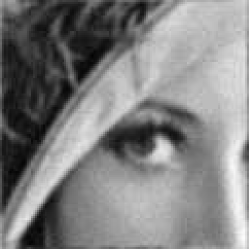
(b)

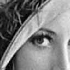
(c)

Figure 23: Example of deconvolution using $\ell^{1}_{N}$ regularization in a frame of translation invariant wavelets. (a) Original $f_{0}$. (b) Observation $y=\Phi f_{0}+w$. (c) Deconvolution $f$.

4.1.5 Source Separation

Sparse representations can be used to separate sources that are known to be sparse in different dictionaries. This corresponds to the morphological component analysis (MCA) of Starck et al. [225]. In its simplest setting, it can be used to separate a single noisy image $y$ into a sum $y=f_{G}+f_{T}+w$ of a cartoon-like component $f_{G}$ (or geometric component), a texture component $f_{T}$ and residual noise $w$. One can use a dictionary $\mathcal{B}=\mathcal{B}_{G}\cup\mathcal{B}_{T}$ union of wavelets ($\mathcal{B}_{G}$) and local cosine ($\mathcal{B}_{T}$), and compute a sparse approximation $f$ of $y$

$$f=\Psi a=\Psi_{G}a_{G}+\Psi_{T}a_{T}$$ (20)

where $a=[a_{G};a_{T}]$ is the solution of the $\ell^{1}_{N}$ basis pursuit (18) applied to $y$. The separation, obtained using $f_{G}=\Psi_{G}a_{G}$ and $f_{T}=\Psi_{T}a_{T}$, is illustrated in Fig. 24.

The modeling of natural images as a sum of a cartoon layer and an oscillating texture layer has been initiated by Y. Meyer in his book [12]. Beside sparsity-based approaches such as (20), other variational methods have been proposed, see for instance the work of J.-F. Aujol et al. [13].

(a)

(b)

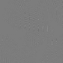
(c)

Figure 24: Example of cartoon+texture decomposition using the MCA algorithm. (a) Original $y$. (b) Geometry layer $f_{G}$. (c) Texture layer $f_{T}$.

4.2 Tree-structured Best Basis Representations

Pursuit algorithms are quite slow and face difficulties in order to compute provably efficient approximations when the dictionary is too redundant. In order to avoid these bottlenecks, one needs to consider more structured representations, that allow one to use fast and provably efficient approximation strategies. The structuring of the representation can be implemented by computing an adapted basis $\mathcal{B}^{\lambda}$ parameterized by a geometric parameter $\lambda$ that captures the local direction of edges or textures. This section details best basis schemes: they introduce the desired adaptivity together with fast algorithms employing the hierarchical structure of parameters $\lambda$.

4.2.1 Quadtree-based Dictionaries

A dictionary of orthonormal bases is a set $\mathcal{D}_{\Lambda}=\{\mathcal{B}^{\lambda}\}_{\lambda\in\Lambda}$ of orthonormal bases $\mathcal{B}^{\lambda}=\{\psi_{\boldsymbol{m}}^{\lambda}\}_{\boldsymbol{m}}$ of $\mathbb{R}^{N}$, where $N$ is the number of pixels in the image. Instead of using an a priori fixed basis such as the wavelet or Fourier basis, one chooses a parameter $\lambda^{\star}\in\Lambda$ adapted to the structure of the image to process and then uses the optimized basis $\mathcal{B}^{\lambda^{\star}}$.

In order to enable the fast optimization of a parameter $\lambda^{\star}$ adapted to a given signal or image $f$ to process, each $\lambda\in\Lambda$ is constrained to be a quadtree. The quadtree $\lambda$ that parameterizes a basis $\mathcal{B}^{\lambda}$ defines a dyadic segmentation of the square $[0,1]^{2}=\bigcup_{(j,i)\in L(\lambda)}S_{j,i}$, where $L(\lambda)$ are the leaves of the trees, as shown on Fig. 25. Each square $S_{j,i}$ is recursively split into four sub-squares $S_{j+1,4i+k}$ for $k=0,\,\cdots,\,3$. In order to enrich the representation parameterized by a quadtree, we attach to each leave of the tree a geometric token, and denote as $\tau$ the number of tokens. A token indicates the direction of the image geometry in a square of the segmentation.

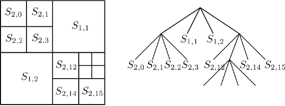
Figure 25: Left: example of dyadic subdivision of $[0,1]^{2}$ in squares $S_{j,i}$ ; right: corresponding quad-tree $\lambda$.

4.2.2 Best Basis Selection

Given a number $M$ of coefficients, the best basis $\mathcal{B}^{\lambda^{\star}}\in\mathcal{D}_{\Lambda}$ adapted to $f\in\mathbb{R}^{N}$ minimizes the best $M$-terms approximation error. This can be equivalently obtained by minimizing a penalized Lagrangian that weights the approximation error with the number of coefficients

$$\lambda^{\star}\in\underset{\lambda\in\Lambda}{\operatorname{argmin}}\;\mathcal{L}(f,\mathcal{B}^{\lambda},T)=\|f-f_{M}^{\lambda}\|^{2}+M^{\lambda}T^{2},$$ (21)

where $f_{M}^{\lambda}$ is the best $M^{\lambda}$-term approximation in $\mathcal{B}^{\lambda}$ computed by thresholding at $T>0$

$$f_{M}^{\lambda}=H_{T}(f,\mathcal{B}^{\lambda},T)=\sum_{|\langle\psi_{\boldsymbol{m}}^{\lambda},\,f\rangle|>T}\langle\psi_{\boldsymbol{m}}^{\lambda},\,f\rangle\psi_{\boldsymbol{m}}^{\lambda}\quad\text{and}\quad M^{\lambda}=\#\left\{\boldsymbol{m}\,:\;|\langle\psi_{\boldsymbol{m}}^{\lambda},\,f\rangle|>T\right\},$$ (22)

since $\mathcal{B}^{\lambda}$ is orthonormal. This Lagrangian can be re-written as a sum over each coefficient in the basis

$$\mathcal{L}(f,\mathcal{B}^{\lambda},T)=\sum_{\boldsymbol{m}}\max(|\langle\psi_{\boldsymbol{m}}^{\lambda},\,f\rangle|^{2},T^{2}).$$ (23)

This kind of Lagrangian can be efficiently optimized using a dynamic search algorithm, originally presented by Coifman et al. [226], which is a particular instance of the Classification and Regression Tree (CART) algorithm of Breiman et al. [227] as explained by Donoho [228]. It is possible to consider other criteria for best basis selection, such as for instance the entropy of the coefficients. This leads different Lagrangians that can be minimized with the same method [226].

The complexity of the algorithm is proportional to the complexity of computing the whole set of inner products $\left\{\langle\psi_{\boldsymbol{m}}^{\lambda},\,f\rangle\,:\;\lambda\in\Lambda\right\}$ in the dictionary. For several dictionaries, such as those considered in this section, a fast algorithm performs this computation in $O(P)$ operations, where $P$ is the total number of atoms in $\mathcal{D}_{\Lambda}$. For tree-structured dictionaries, this complexity is thus $O(\tau N\log_{2}(N))$, where $\tau$ is the number of tokens associated to each leaf of the tree. This is much smaller than the total number of basis $\mathcal{B}^{\lambda}$ in $\mathcal{D}_{\Lambda}$, that grows exponentially with $N$.

4.2.3 Wavelet and Cosine Packets

A basis $\mathcal{B}^{\lambda}$ with oscillating atoms is defined using a separable cosine basis over each square of the dyadic segmentation. In this case no geometry is used, the oscillation of the atoms does not follow the geometry of the image, and $\tau=1$. An approximation in an adapted cosine basis $\mathcal{B}^{\lambda}$ allows one to capture the spatial variations of a texture [33].

A wavelet packet basis $\mathcal{B}^{\lambda}$ defines a dyadic subdivision of the $2$-D frequency domain [229]. The projection of an image on the atoms of $\mathcal{B}^{\lambda}$ is computed through a pyramidal decomposition that generalizes the orthogonal wavelet transform, adding flexibility to overcome its dyadic frequency decomposition. Uniform dyadic wavelet packet decompositions generate a subset of $M$-band wavelets with equal-span frequency subbands obtained from $J$ decomposition levels, with $M=2^{J}$. In order to adapt to the specific frequency content of the image, the resulting tree is parsed through a best basis selection procedure [226], reminiscent of the subdivision in Fig. 25.

This construction is generalized by considering non-stationary wavelet packets [230], that apply different quadrature mirror filters at each scale of the tree. A dynamic programming algorithm detailed in [231] computes an adapted non-stationary basis.

4.2.4 Adaptive Approximation

Wedgelets

A geometric approximation is obtained by considering for each node of the dyadic segmentation a collection of $\tau$ different low-dimensional discontinuous approximation spaces [232]. For each node of the quadtree, a token indicates the local direction and position of the edge. The low-dimensional approximation spaces are piecewise polynomials over each of the two wedges.

The wedgelets introduced by Donoho [232] rely on piecewise constant approximation. This scheme is efficient when approximating a piecewise constant image $f$ whose edges are $\text{C}^{2}$ curves. For such cartoon images, the approximation error decays like $\|f-f_{M}\|^{2}=M^{-2}$, see [232, 21]. It is also possible to consider approximation spaces with higher-order polynomials in order to capture arbitrary cartoon images [233], see also [234] for a related construction. The computation of the low-dimensional projection can be significantly accelerated, see [235].

The piecewise constant model for images being relatively simplistic, wedgelets have been upgraded to platelets [236] and surflets [237]. They aim at improving the management of smooth intensity variations, since they rely on planar or even smoother approximation on dyadic square or wedge based grids.

Bandlets

For coding, orthogonal expansions are preferred over low-dimensional approximations as considered by wedgelets. Switching to non-linear approximation in bases also better handles directional textures that do not correspond to a fixed low-dimensional space parameterized by a wedge.

The bandlet bases dictionary is introduced by Le Pennec and Mallat [238]. Bandlets perform an efficient adaptive approximation of images with geometric singularities. An anisotropic basis with a preferred orientation is defined over each square of the dyadic segmentation. Fig. 26 (a) shows an example of bandlet atom. The orientation is parameterized with the token stored in the leaf of tree. Keeping only a few bandlet coefficients and setting the others to zero performs an approximation of the original image that follows the local orientation indicated by the token.

(a)

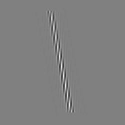
(b)

Figure 26: Example of a bandlet atom. (a) Atom in the spatial domain. (b) Wavelet-bandelet atom.

Adaptive Approximation over the Wavelet Domain

Applying such an adaptive geometric approximation directly on the image leads to unpleasant visual artifacts. In order to overcome this issue, one applies a tree-structured approximation or a best basis computation on the discrete set of wavelet coefficients. The wedgeprint of Wakin et al. [239] uses a vector quantization to extend the wedgelet scheme to the wavelet domain. The second generation bandlets of Peyré and Mallat [240] use an adaptive bandlet basis for each scale of the wavelet transform. All these methods benefit from the same approximation error decay as their single scale predecessors, but work better in practice.

Fig. 26 shows how a bandlet atom (a) is mapped to a wavelet-bandlet atom (b). Decomposing an image over a bandlet basis composed of atoms of type (b) is equivalent to applying first a wavelet transform, and then decomposing the wavelet coefficients over atoms of type (a).

Another adaptive approximation relying on the processing of the wavelet domain is the easy path wavelet transform (EPWT) [241]. It provides a hybrid and adaptive approach exploiting the local correlations of images along path vectors through index subsets in the Wavelet domain.

4.2.5 Adaptive Tree-structured Processing

For compression and denoising applications, one computes the best basis $\mathcal{B}^{\lambda^{\star}}$ adapted to the image $f$ to compress or denoise by minimizing the corresponding Lagrangian (23). The coefficients $\langle\psi_{\boldsymbol{m}}^{\lambda},\,f\rangle$ are then binary coded (for compression) or thresholded (for denoising). The resulting improvement of the best basis approximation error over wavelets translates into improvement in the rate distortion (for compression) or average risk (for denoising) of the best basis method, see for instance [239, 240].

One can also use best bases to recover an image from noisy low-dimensional measurements $y=\Phi f+w$ where $\Phi$ is an ill-conditioned linear mapping. For some problems such as inpainting, small missing regions or light blur removal, the best basis $\lambda$ can be estimated directly from the observation $y$.

An example of inverse problem where sparsity in a best basis significantly improves over sparsity in a fixed basis is compressed sensing. Compressed sensing is a new data sampling strategy, where the measurement operator $\Phi$ of size $P\times N$ is generally the realization of some random matrix ensemble. The sampling operations $y=\Phi f+w\in\mathbb{R}^{P}$ allows one to acquire a high resolution signal $f\in\mathbb{R}^{N}$ directly in a compressed format of $P<N$ measurements. Compressed sensing theory ensures that if the number of measurements $P$ is large enough with respect to the sparsity $K$ of the signal $f$ in a basis $\mathcal{B}$, typically, $P=O(K\log N/K)$ for Gaussian random matrix $\Phi$, one recovers a good approximation of the signal using a $\ell^{1}_{N}$ sparse regularization as in (19). It can be shown that the quality of the reconstruction depends both on the sensing noise power $\|w\|$ and on the “compressibility” of $f$, that is, its deviation from the strictly sparse case. We refer to the review paper of Candès [242] and the references therein for more details. Fig. 27 shows a comparison of compressed sensing recovery from $P=N/6$ measurements using a redundant frame $\mathcal{B}$ of translation invariant wavelets, and a best bandlet basis. In this last result, it is necessary to use an iterative algorithm that progressively improves the quality of the estimated geometry, see [243]. As explained in this last reference, the same technique can be used for inpainting large holes in images.

Figure 27: (a,a’) original image ; (b) compressed sensing reconstruction using a translation invariant wavelet frame (PSNR=37.1dB) ; (c) reconstruction using a best bandlet basis (PSNR=39.3dB). (b’) wavelet frame, PSNR=22.1dB, (c’) bandlet basis, PSNR=23.9dB.

4.2.6 Adaptive Segmentations and Triangulations

In order to enhance the quality of the representation, it is possible to consider tree-structured segmentations $[0,1]^{2}=\bigcup_{\beta\in\lambda}\beta$ of the image where the boundaries of the sub-domains $\beta\in\lambda$ are not restricted to be axis-aligned. The advantage is that such an adaptive segmentation defines regions $\beta\in\lambda$ with arbitrary complicated boundaries. Unfortunately, the combinatorial explosion of the set of all possible $\lambda$ forbids the search for an optimal segmentation with a fast algorithm. One has thus to use a greedy scheme that selects at each step a split to reduce the approximation error.

Recursive Splitting and Approximation Spaces

A greedy scheme computes an embedded segmentation $\lambda=\{\lambda_{j}\}_{j}$, where $\lambda_{j+1}\subset\lambda_{j}$ is obtained by splitting a region $\beta\in\lambda_{j}$. The full segmentation $\lambda$ can thus be represented and coded using a binary tree. This defines multiresolution spaces $V_{\lambda_{j+1}}\subset V_{\lambda_{j}}$ where $V_{\lambda_{j}}$ is composed, for instance, of piecewise polynomial functions on each region $\beta\in\lambda_{j}$.

It is possible to compute a single-scale orthogonal projection $f_{M}=P_{V_{\lambda_{j}}}(f)$ of an image $f$ on a fixed resolution space $V_{\lambda_{j}}$ in order to perform image approximation or compression. It is also possible to define a detail space $V_{\lambda_{j+1}}=V_{\lambda_{j}}\oplus W_{\lambda_{j}}$. A wavelet basis $\mathcal{B}^{\lambda}$ can be built by considering a basis for each $W_{\lambda_{j}}$. A non-linear thresholding approximation $f_{M}=H_{T}(f,\mathcal{B}^{\lambda},T)$ provides an additional degree of adaptivity and reduces the approximation error $\|f-f_{M}\|$. Wavelet bases on adaptive segmentations also enable a progressive coding of the coefficients by decaying $T$, which is important for image compression applications.

Adaptive Segmentation

A popular splitting rule is the binary space tiling, that splits a region $\beta\in\lambda_{j}$ according to a straight line, see for instance [244].

Other popular approaches restrict the regions $\beta\in\lambda_{j}$ to triangles, so that $\lambda_{j}$ is a triangulation of the domain $[0,1]^{2}$. It is possible to refine the triangulation by adding new vertices, or on the contrary to remove vertices to go from $\lambda_{j+1}$ to $\lambda_{j}$. These vertex-based schemes do not satisfy $\lambda_{j+1}\subset\lambda_{j}$, so one cannot build a wavelet basis using such triangulations. These vertex refinement methods generate a single scale approximation $P_{V_{\lambda_{j}}}(f)$ and lead to efficient image coders, see for instance [245].

To generate embedded approximation spaces $\lambda_{j+1}\subset\lambda_{j}$, one needs to split the triangles $\beta\in\lambda_{j}$. Regular split of orthogonal triangles leads to isotropic adaptive triangulations [246]. Splitting triangles according to a well chosen median leads to anisotropic triangulations that exhibit optimal aspect ratio for smooth images, see [247]. More complicated, non-linear coding schemes are possible, for instance using normal meshes [248], that treat an image as an height field.

4.3 Lifting Representations

To enhance the wavelet representation, the wavelet filters can be adapted to the image content. The lifting scheme, popularized by Sweldens [249] and latent in earlier works [250, 251, 252], is an unifying framework to design adaptive biorthogonal wavelets, through the use of spatially varying local interpolations. While it can typically reduce the computation of the wavelet transform by a factor of about two in $1$-D, it also guarantees perfect reconstruction for arbitrary filters, and can be used (Sec. 5.3) on non-translation invariant grids to build wavelets on surfaces, see Sec. 5.

4.3.1 Lifting Scheme

At each scale $j$, the scaling coefficients $a_{j-1}$ are evenly split into two groups $a_{j}^{o}$ and $d_{j}^{o}$. The wavelet coefficients $d_{j}$ and the coarse scale coefficients $a_{j}$ are obtained by applying linear operators $P_{j}^{\lambda_{j}}$ and $U_{j}^{\lambda_{j}}$ parameterized by ${\lambda_{j}}$

$$d_{j}=d_{j}^{o}-P_{j}^{\lambda_{j}}a_{j}^{o}\quad\text{and}\quad a_{j}=a_{j}^{o}+U_{j}^{\lambda_{j}}d_{j}.$$ (24)

The resulting lifted wavelet coefficients $\{d_{j}\}_{j}$ are thresholded or quantized to achieve denoising or compression. These two lifting or ladder steps are easily inverted by reverting the order of the operations. The predictor $P_{j}^{\lambda_{j}}$ interpolates the sub-sampled values $a_{j}^{o}$ in order to reduce the amplitude of the wavelet coefficients $d_{j}$, while the update mapping $U_{j}^{\lambda_{j}}$ stabilizes the transform by maintaining certain quantities such as the mean of the scaling coefficients. By applying sequentially several predict and one update operators, one can recover arbitrary biorthogonal wavelets on uniform $1$-D grid [253], speeding up the wavelet decomposition algorithm by a factor of about two in $1$-D. The lifting structure in Fig. 28(a) corresponds to the 5/3 lifted wavelet. Such structures may furthermore adapt to non-linear filters and morphological operations [254, 255]. An example of lifting based quincunx scheme example from [256, 257] is displayed in Fig. 28(b).

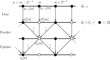
(a)

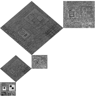
(b)

Figure 28: (a) Predict and update lifting steps (b) MaxMin lifting of the Haar-Riesz Memorial plaque.

4.3.2 Adaptive Predictions

It is possible to design the set of parameter $\lambda=\{\lambda_{j}\}_{j}$ to adapt the transform to the geometry of the image. We call $\lambda_{j}$ an association field, since it typically links a coefficient of $a_{j}^{o}$ to a few neighboring coefficients in $d_{j}^{o}$. Each association is optimized to reduce, as much as possible, the magnitude of wavelet coefficients $d_{j}$, and should thus follow the geometric structures in the image. One can compute these associations to reduce the length of the wavelet filter near the edges, using the information from the coarser scale [258]. Locally adaptive schemes have proven efficient in stereo and video coding [259, 260, 261, 262].

Such schemes are related to adaptive non-linear subdivision [263]. To further reduce the distortion of geometric images, the orientations of the association fields $\{\lambda_{j}\}_{j}$ can be optimized though the scales. Because of the lack of structure of the set of bases $\mathcal{B}^{\lambda}$, computing the field $\lambda_{j}$ that produces the best non-linear approximation is intractable. These flows are thus usually computed using heuristics to detect the local orientation of edges, see for instance [264, 265, 165, 266]. These adaptive lifting schemes are extended to perform adaptive video transforms where the lifting steps operate in time by following the optical flow $\lambda_{j}$, see for instance [267, 268].

4.3.3 Grouplets

A difficulty with lifted transforms is that they do not guarantee the orthogonality of the resulting wavelet frame. The stability of the transform thus tends to degrade for complicated association fields $\{\lambda_{j}\}_{j}$. The grouplet transform, introduced by Mallat [269], also makes use of association fields, but it replaces the lifting computation of wavelet coefficients by an extended Haar transform, where coefficients in $d_{j}^{o}$ are processed in sequential order to maintain orthogonality.

Grouplets defined over each scale of the wavelet transform have been used to perform image denoising, super-resolution [269] and inpainting [270] by solving a $\ell^{1}_{N}$ regularization similar to (19). Grouplets can also be used to solve computer graphics problems such as texture synthesis. Classical approaches to texture synthesis use statistical models over a fixed representation such as a wavelet basis, see for instance [271, 272]. Building similar statistical models over a grouplet basis [270] allows one to better synthesize the geometry of some textures, and gives results similar to state of the art computer graphics approaches such as texture quilting [273]. Furthermore, the explicit parameterization of the geometry though the association fields $\lambda$ allows the user to modify this geometry and synthesize dynamic textures. A comparison of these different approaches on one texture synthesis example is given in Fig. 29.

(a)

(b)

(c)

(d)

Figure 29: Example of texture synthesis by statistical modeling of grouplet coefficients. (a) Exemplar. (b) Wavelet [272]. (c) Quilting [273]. (d) Grouplets [270].

5 Transformations on Non-Euclidean Geometries

In this section we describe how the concepts of frequency, scale and even directionality have been extended to the processing of data on non-euclidean geometries like the sphere and other manifolds.

5.1 Data Processing on the Sphere

The unit sphere $S^{2}=\{\boldsymbol{x}\in\mathbb{R}^{3}:\|\boldsymbol{x}\|=1\}\subset\mathbb{R}^{3}$ is one of the most natural non-Euclidean spaces. Very early, possibly due to influences for astronomy and geosciences, many data processing techniques have been developed for this surface. Many filtering, multiscale, directional and hierarchical methods have been designed, either in the spherical frequency domain induced by the spherical harmonics basis — often following the spirit of some Euclidean techniques exposed in the previous sections — or on the sphere itself thanks to some geometrical tools such as the stereographic dilation or the lifting schemes for wavelet analysis.

5.1.1 Filtering

As for the plane, filtering operations may be defined on $S^{2}$. Given the common two-angle spherical parameterization $\boldsymbol{\xi}=(\theta,\varphi)\in S^{2}$ with the co-latitude $\theta\in[0,\pi]$ and longitude $\varphi\in[0,2\pi)$, this operation is realized through spherical convolution evaluated on ${\rm SO}(3)$ (the group of rotations in $\mathbb{R}^{3}$). For a function $f\in\mathbb{L}^{2}(S^{2})=\{g:\|g\|^{2}_{2}=\int_{S^{2}}|g|^{2}<\infty\}$ and a filter $h\in\mathbb{L}^{2}(S^{2})$, the convolution is

$$(f\star h)(\boldsymbol{\rho})\ =\ \int_{S^{2}}\ h(\boldsymbol{\rho}\,\boldsymbol{\xi})f(\boldsymbol{\xi})\ {\rm d}\mu(\boldsymbol{\xi}),$$

where $\boldsymbol{\rho}\in{\rm SO}(3)$ is a rotation (driven by three angles) applied to the point $\boldsymbol{\xi}\in S^{2}$ and ${\rm d}\mu(\boldsymbol{\xi})=\sin\theta{\rm d}\theta{\rm d}\varphi$. For an axisymmetric filter, i.e., if $h(\boldsymbol{\xi})=h(\theta)$, the convolution reduces to $(f\ast h)(\boldsymbol{\xi}^{\prime})\ =\ \int_{S^{2}}\ h(\boldsymbol{\xi}^{\prime}\cdot\boldsymbol{\xi})f(\boldsymbol{\xi})\ {\rm d}\mu(\boldsymbol{\xi})$, where $\boldsymbol{\xi}^{\prime}\cdot\boldsymbol{\xi}$ is the common 3-D scalar product between $\boldsymbol{\xi}^{\prime}$ and $\boldsymbol{\xi}$ seen as unit vectors.

5.1.2 Fourier Transform

The Fourier transform of a function $f\in\mathbb{L}^{2}(S^{2})$ is defined by

$$\hat{f}_{\ell m}=\langle Y_{\ell m},f\rangle=\int_{S^{2}}Y_{\ell m}^{*}(\boldsymbol{\xi})\,f(\boldsymbol{\xi})\ {\rm d}\mu(\boldsymbol{\xi}),\quad f(\boldsymbol{\xi})=\sum_{\ell,m}\hat{f}_{\ell m}\,Y_{\ell m}(\boldsymbol{\xi})$$

with respect to orthonormal basis of spherical harmonics $\mathcal{Y}=\{Y_{\ell m}(\boldsymbol{\xi}):\ell\geqslant 0,|m|\leqslant\ell\}$, i.e., the eigenvectors of the spherical Laplacian [274].

The frequency content of $f$ is thus represented by the value of $\hat{f}_{\ell m}$ on the order $\ell\in\mathbb{N}$, which basically counts the number of oscillations on the latitudes, and the moment $m\in\{-\ell,\cdots,\ell\}$ counting longitude oscillations. Numerically, only certain discretizations of the sphere can provide perfect quadrature formulae to compute the Fourier coefficients of band-limited functions on the sphere, sometimes with very efficient algorithms [274, 275].

5.1.3 Spherical Scale-Space

Similarly to what happened for signals or images, the first notion of “scale” on the sphere was imported from the Heat Dynamic that is also known on this space. In that framework, if a spherical function $f\in\mathbb{L}^{2}(S^{2})$ is considered the initial heat configuration, the spherical heat dynamics smooth it with time $\tau>0$, conferring a scaling notion on this parameter.

Interestingly, as for Euclidean spaces, the solution at time $\tau>0$ of the heat equation initialized to some function $f\in\mathbb{L}^{2}(S^{2})$ is simply $f(\boldsymbol{\xi},\tau)=\sum_{\ell,m}\hat{f}_{\ell m}(\tau)Y_{\ell m}(\boldsymbol{\xi})$, with $\hat{f}_{\ell m}(\tau)=\hat{f}_{\ell m}\,e^{-\ell(\ell+1)\,\tau}$ and $f(\boldsymbol{\xi},0)=f(\boldsymbol{\xi})$. Alternatively, since for an axisymmetric filter $h$ we have the spherical convolution theorem

$$\widehat{(f\ast h)}_{\ell m}\ =\ \textstyle\sqrt{\tfrac{4\pi}{2\ell+1}}\,\hat{f}_{\ell m}\,\hat{h}_{l0},$$

the solution of the Heat Equation can also be obtained by a convolution by a specific kernel $G^{\circ}_{\tau}(\boldsymbol{\xi})$, coined spherical Gaussian of width ${\sqrt{\tau}}$. It is defined in frequency by $\widehat{(G^{\circ}_{\tau})}_{\ell m}=\sqrt{{(2\ell+1)}/{4\pi}}\,e^{-\ell(\ell+1)\,\tau}$.

The link between the heat dynamics and the spherical convolution with the axisymmetric filter $G^{\circ}_{\tau}$ has been exploited by Bülow [276] to develop several specific spherical filters for feature detection, such as the Laplacian of Gaussian or the directional derivative of Gaussian.

5.1.4 Spectral Wavelets

Freeden et al. [277, 278] have fully exploited the connection between convolution and frequency filtering on the sphere to develop a continuous wavelet transform on the sphere. This is done by introducing a family of axisymmetric functions $\psi_{a}(\boldsymbol{\xi})$, coined spherical wavelet, continuously indexed by $a>0$, and such that $\int_{\mathbb{R}_{+}}|\widehat{(\psi_{a})}_{\ell 0}|^{2}\ {\rm d}a/a=1$, $\widehat{(\psi_{a})}_{00}=0$, plus additional regularity conditions. The wavelet coefficients of a function $f\in\mathbb{L}^{2}(S^{2})$ are then defined as $W_{f}(a,\boldsymbol{\xi})=(f\ast\psi_{a})(\boldsymbol{\xi})$. The reconstruction is possible (almost everywhere) by

$$f(\boldsymbol{\xi}^{\prime})\ =\ \langle f\rangle\ +\ \int_{\mathbb{R}_{+}}\int_{S^{2}}\ W_{f}(a,\boldsymbol{\xi})\,\psi_{a}(\boldsymbol{\xi}^{\prime}\cdot\boldsymbol{\xi})\ \tfrac{{\rm d}a}{a}\,{\rm d}\boldsymbol{\xi},$$

with $\langle f\rangle={\textstyle\frac{1}{4\pi}}\int_{S^{2}}f(\boldsymbol{\xi})\,{\rm d}\mu(\boldsymbol{\xi})$.

In [277, 278], an MRA on the sphere is also built by defining Quadrature Mirror Filters in the frequency domain. A spatial sub-sampling of the different subspaces of the MRA can also decrease the redundancy of the basis hence created.

Following a similar approach, (isotropic) needlet frames introduced in [279, 280, 281] represent another example of spectral wavelets, i.e., wavelets shaped in the Fourier domain. Needlets additionaly offer relationships with quadrature formulae used to turn integrals of bandlimited functions into discrete summations.

5.1.5 Stereographic Wavelets

In the previous sections, the notion of scale in the processing of spherical data was always defined in the frequency domain, i.e., by dilating the frequency domain by a parameter, preventing a fine control of the spatial support of the filter.

An alternative approach introduced by Antoine and Vandergheynst [282, 283] defines the dilation directly in the spatial domain. The compactness of $S^{2}$ is respected, by introducing a stereographic dilation. As illustrated on Fig. 30-(a) for point dilation, the stereographic dilation $D_{a}$ of a function $g\in\mathbb{L}^{2}(S^{2})$ amounts to projecting $g$ on the plane tangent at the North Pole by the stereographic projection $\Pi$, to applying there a Euclidean dilation $d_{a}$ by a scale $a>0$, and to lifting the resulting function back to the sphere by $\Pi^{-1}$ [284]. Mathematically, $[D_{a}g](\theta,\varphi)=\lambda(a,\theta)\,g(\theta_{1/a},\varphi)$, with $\tan\theta_{\alpha}/2=\alpha\tan\theta/2$ and where $\lambda$ is a normalizing function such that $\|D_{a}g\|_{2}=\|g\|$.

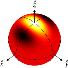
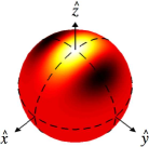
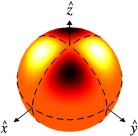
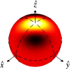
Figure 30: (a) Stereographic dilation on $S^{2}$. On the right, the (steerable) second directional derivative of Gaussian. The three images (b)-(d) are the basis elements, while the fourth in (e) is a linear combination of the first three yielding a rotation of $\pi/4$ around the North pole.

Given a mother wavelet $\psi\in\mathbb{L}^{2}(S^{2})$ centered on the North pole, the proposed approach considers the joint action of translations, i.e., rotation operators $R_{\boldsymbol{\rho}}$ in ${\rm SO}(3)$, and of the dilations $D_{a}$ on $\psi$. The wavelet transform of $f$ is therefore:

$$W_{f}(\boldsymbol{\rho},a)\ =\ \langle\psi_{(\boldsymbol{\rho},a)},f\rangle,\quad\boldsymbol{\rho}\in{\rm SO}(3),\ a>0,$$

with $\psi_{(\boldsymbol{\rho},a)}=R_{\boldsymbol{\rho}}D_{a}\psi$. If the wavelet is admissible, which is nearly equivalent to impose $\int_{S^{2}}\,{\rm d}\mu(\theta,\varphi)\ \tfrac{\psi(\theta,\varphi)}{1+\cos\theta}=0$, the reconstruction of $f$ is possible through

$$f(\boldsymbol{\xi})\ =\ \langle f\rangle\ +\ \int_{\mathbb{R}_{+}^{*}}\int_{{\rm SO}(3)}\tfrac{{\rm d}a{\rm d}\nu(\boldsymbol{\rho})}{a^{3}}\ W_{f}(\boldsymbol{\rho},a)\,[R_{\boldsymbol{\rho}}L_{\psi}^{-1}D_{a}\psi](\boldsymbol{\xi}),$$

where $\nu$ is the Lebesgue measure on ${\rm SO}(3)$ and $L_{\psi}$ is a multiplicative operator function of $\psi$ only and expressed in the Fourier domain [282]. For axisymmetric wavelets, this result simplifies by the fact that the action of $R_{\boldsymbol{\rho}}$ on $\psi$ is controlled by two angles only.

Many wavelets may be defined on the sphere since it has been proved in [284] that any admissible wavelet on the plane $\mathbb{L}^{2}(\mathbb{R}^{2})$ can be imported by inverse stereographic projection $\Pi^{-1}$. A Laplacian of Gaussian (LoG), difference of Gaussians (DoG), Morlet Wavelet, and many other are generally used [282, 285, 286]. Numerically, this spherical CWT is obtained thanks to the convolution theorem mentionned previously. This transform has been for instance intensively used in the analysis of the Cosmic Microwave Background (CMB), an astronomical signal remnant of some specific evolution phase of the Big Bang [287, 288, 289].

Wavelet frames can be developed in this theory by discretizing the scaling parameter $a$ [285]. These frames, that do not subsample the spherical positions, have successfully served for the construction of invertible filter banks on the 2-Sphere [290] even if the stereographic dilation is not really compatible with the frequency description of the wavelets.

5.1.6 Haar Transform on the Sphere

The constructions of spherical wavelets described in the previous section make use of the Fourier decomposition on the sphere. It is possible to define wavelets directly over the spherical domain without Fourier analysis, using for instance the lifting scheme method [291], see Sec. 5.3. This allows one to define spherical wavelets with a compact support, although the stability of the resulting transform is more difficult to control than over the planar domain.

Inspired by this lifting scheme [291], one can easily define a Haar basis on the sphere by considering a family $\{\mathcal{M}^{j}\}_{J\leqslant j\leqslant 0}$ of embedded spherical triangulations that approximate a sphere [292]. These triangulations are obtained by a regular 1:4 refinement rule starting from an initial regular polyhedron $\mathcal{M}^{0}$, and the edges are projected on the sphere to define spherical triangles.

The corresponding spherical multiresolution defines $V_{j}\subset\mathbb{L}^{2}(S^{2})$ as the set of functions that are constant on each triangle of $\mathcal{M}^{j}$. Figure 31 shows the linear projection of a spherical function on some of these multiresolution spaces.

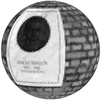
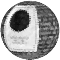
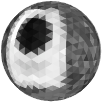
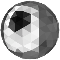
$j=5$	$j=4$	$j=3$	$j=2$

Figure 31: Projection on the spherical Haar multiresolution.

Following the usual definition (Sec. 2.3.1), a Haar wavelet basis $\{\psi_{j,n}\}_{n}$ is an orthogonal basis of the detail space $W_{j}$ such that $V_{j+1}=V_{j}\oplus W_{j}$. The wavelet coefficients $\langle\psi_{j,n},\,f\rangle$ are computed using a pyramid algorithm that mimics the usual Haar transform, except that for each triangle, one gathers three detail coefficients and one coarse scale coefficient. Figure 32 shows these Haar coefficients together with a comparison between spherical and planar non-linear approximations $H_{T}(f)$.

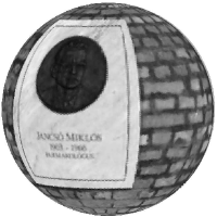
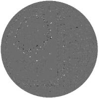
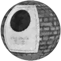
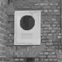
$f$	$\{\langle\psi_{j,n},\,f\rangle\}_{j,n}$	$H_{T}(f)$ (spherical)	$H_{T}(f)$ (planar)

Figure 32: Comparison of spherical and planar Haar approximations. The threshold $T$ is adjusted so that $H_{T}(f)$ is an approximation with a number of coefficients equal to $5\%$ of the number of pixels in the high resolution planar image.

5.1.7 Steerable Wavelets on the Sphere

Finally, the sphere is compatible with the definition of steerable filters similarly to those defined in Sec. 3.2.2 for the plane. In particular, using the stereographic projection $\Pi$ introduced in the previous section, steerability on the sphere is also imported from the plane. This fact has been used in [284, 293, 294] to define differential and steerable filters useful to detect directional features in the Cosmic Microwave Background. An example of a steerable wavelet is given in Fig. 30(b-e). Spherical steerability may also be directly studied in the frequency domain with spectral dilation [295].

5.1.8 Other Constructions

It is impossible to cite the vast literature on multiscale decomposition on the sphere. Let us just quote some of them. Wavelets, ridgelets and curvelets have been translated on the sphere by Starck et al. [296] by using a particular spherical sampling, called HEALPix, locally similar to a square discretization. Locally supported biorthogonal wavelet bases have been also realized thanks to some radial projections of the planar faces of a cube on $S^{2}$ in [297].

5.2 Wavelets on General 2-Manifolds

Given a two-dimensional manifold $\mathcal{M}$, i.e., locally isomorphic to $\mathbb{R}^{2}$, authors in [298] describe how to define a Continuous Wavelet Transform (CWT) for function $f:\mathcal{M}\to\mathbb{C}$.

Similarly to the way the stereographic dilation is defined for the sphere, the local dilation of a function $\psi$ around the point $\boldsymbol{\xi}\in\mathcal{M}$ relies on the knowledge of a local and invertible projection $\Pi_{\boldsymbol{\xi}}$ between $\mathcal{M}$ and its tangent plane $T_{\boldsymbol{\xi}}\mathcal{M}$ on $\boldsymbol{\xi}$. The desired dilation of scale $a>0$ therefore factorizes as $D_{(\boldsymbol{\xi},a)}=\Pi_{\boldsymbol{\xi}}^{-1}d_{a}\Pi_{\boldsymbol{\xi}}$ with $d_{a}$ the common Euclidean dilation of function in $T_{\boldsymbol{\xi}}\mathcal{M}\simeq\mathbb{R}^{2}$.

Given the Hilbert space $\mathcal{H}=\mathbb{L}^{2}(\mathcal{M},{\rm d}\mu)$ of square integrable function on $\mathcal{M}$, for a proper measure ${\rm d}\mu$, the CWT of a function $f$ on $\mathcal{M}$ is then formally defined by correlating $f$ with a set of prototype wavelets $\psi_{(\boldsymbol{\xi})}\in\mathcal{H}$ localized around any $\boldsymbol{\xi}\in\mathcal{M}$, i.e.,

$$W_{f}(\boldsymbol{\xi},a)\ =\ \langle\psi_{(\boldsymbol{\xi},a)},f\rangle_{\mathcal{H}}\ \triangleq\ \int_{\mathcal{M}}\,{\rm d}\mu(\boldsymbol{\xi}^{\prime})\ f(\boldsymbol{\xi}^{\prime})\,\psi_{(\boldsymbol{\xi},a)}(\boldsymbol{\xi}^{\prime}),\qquad\psi_{(\boldsymbol{\xi},a)}=D_{(\boldsymbol{\xi},a)}\psi_{(\boldsymbol{\xi})}.$$

The theoretical invertibility of this transform has however to be studied specifically in each case, i.e., given $\mathcal{M}$ and $\Pi_{\boldsymbol{\xi}}$. Results exist for instance for the two-sheeted hyperboloid and the paraboloid in $\mathbb{R}^{3}$ [299].

5.3 Lifting Scheme Wavelets on Meshed Surfaces

The lifting scheme of Sweldens [300], described in Sec. 4.3, can be used to define wavelets on non-translation invariant geometries, including surfaces with complicated topologies. Lifted wavelets on surfaces are usually built on a semi-regular mesh grid, was first considered by Lounsbery et al. [301], and then refined within the lifting framework by Schröder and Sweldens [291].

Semi-regular meshes $\{\mathcal{M}^{j}\}_{J\leqslant j\leqslant 0}$ are obtained by a regular 1:4 refinement rule starting from an arbitrary control mesh $\mathcal{M}^{0}$. Each edge of $\mathcal{M}^{j}$ is split into two sub-edges by vertex insertion to obtain the refined mesh $\mathcal{M}^{j-1}$. The fine mesh $\mathcal{M}^{J}$ is the sampling grid that stores the position of the surface points in space, and a signal $f$ sampled at each grid point. Fig. 33, top row, shows an example of such a multiresolution mesh, obtained by a semi-regular remeshing of a high resolution input mesh.

The lifting scheme described in Sec. 4.3 can be applied by storing the scaling coefficients $a_{j}$ on the grid point of the mesh $\mathcal{M}^{j}$, while the detail coefficients are stored on the complementary detail grid $\mathcal{D}^{j}$ where $\mathcal{M}^{j-1}=\mathcal{M}^{j}\cup\mathcal{D}^{j}$. The splitting of $a_{j-1}$ into $a_{j}^{o}$ and $d_{j}^{o}$ corresponds to assigning the values stored in $\mathcal{M}^{j-1}$ to either $\mathcal{M}^{j}$ or $\mathcal{D}^{j}$. The predict operator $P_{j}$ used to compute the wavelet coefficients $d_{j}$ stored in $\mathcal{D}^{j}$ is a local polynomial interpolator on a triangulation grid. The update operator $U_{j}$ is computed by solving a linear system, to impose that moments of low orders, such as the mean, are preserved when moving from $a_{j-1}$ to $a_{j}$.

This lifting wavelet transform computes the coefficients $d_{j}[\boldsymbol{n}]=\langle\psi_{(j,\boldsymbol{n})},\,f\rangle$ for all scales $0<j<J$ and grid points $\boldsymbol{n}\in\mathcal{D}^{j}$. It corresponds to the projection of the signal $f$ defined on the triangulated surface $\mathcal{M}^{j}$ onto a discrete biorthogonal wavelet frame $\mathcal{B}=\{\psi_{(j,\boldsymbol{n})}\}_{j,\boldsymbol{n}}$. These coefficients can be thresholded, and inverting the lifting steps creates an approximated signal $f_{M}$ with $M$ non-zero coefficients. Although this approach works well in practice, the frame bounds of the resulting wavelet frame $\mathcal{B}$ are difficult to control, and $f_{M}$ might be far from the best $M$-terms approximation. It is also difficult to guarantee the convergence of the wavelet atoms $\psi_{(j,\boldsymbol{n})}$ to smooth functions, when $J$ tends to $-\infty$, and the mesh $\mathcal{M}^{J}$ approximates a smooth surface.

To perform surface approximation, one defines the signal $a_{J}$ at the finest scale as the position of the nodes on the surface. Each coefficient $a_{J}[\boldsymbol{n}]\in\mathbb{R}^{3}$ is thus a point in 3D space. The lifting transform can be applied to this vector-valued signal. Thresholding the resulting wavelet coefficients allows one to approximate the surface using few coefficients, as shown on Fig. 33, bottom row. If the lifting operators $P_{j}$ and $U_{j}$ do not depend on the position of the points on the surface, the resulting lifting wavelets can be used to perform 3D mesh compression [301, 291].

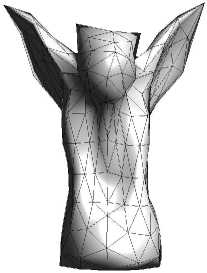
(a)

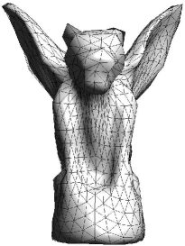
(b)

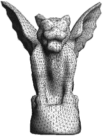
(c)

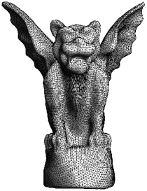
(d)

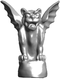
(e)

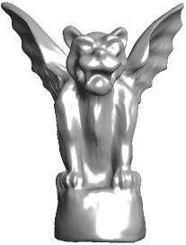
(f)

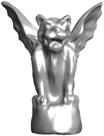
(g)

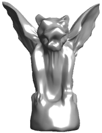
(h)

Figure 33: Top row: example of semi-regular mesh $\{\mathcal{M}^{j}\}_{j}$. Bottom row: example of surface approximation $f_{M}$ obtained by thresholding the lifted wavelets coefficients, where $N$ is the number of vertices in $\mathcal{M}^{J}$. (a) $\mathcal{M}^{j},j=-4$. (b) $\mathcal{M}^{j},j=-5$. (c) $\mathcal{M}^{j},j=-6$. (d) $\mathcal{M}^{j},j=-7$. (e) $M/N=100\%$. (f) $M/N=10\%$. (g) $M/N=5\%$ (h) $M/N=2\%$.

5.4 Wavelets on Graphs

Let us finally mention that wavelet transform has been extended to functions defined on the vertices of an arbitrary finite weighted graph. The latter may for instance generalize standard picture definition by describing two-dimensional pixel adjacencies. Maggioni et al. introduced “diffusion wavelets” [302], a general theory for wavelet decompositions based on compressed representations of powers of a diffusion operator such as the graph Laplacian. The constructed wavelet basis is made orthogonal by combining graph subsampling and Gram-Schmidt orthogonalization on each subsampled space.

More recently, Hammond et al. [303] developed a general wavelet frame theory on such graphs thanks to the graph analogue of the Fourier domain, namely the spectral decomposition of the discrete graph Laplacian. Wavelets are defined in this frequency domain by dilating an “admissible” generating kernel. The final representation is redundant but wavelets can be shaped by changing the generating kernel. Moreover, for sparse graph Laplacian matrix, a fast wavelet transform avoiding the Laplacian spectral decomposition is developed.

6 Conclusion

A century after the discovery by Alfréd Haar, and twenty years after the emergence of wavelets as genuine processing tools, major advances have been made in the improvement of natural images representations, aiming at enhanced understanding.

Their common characteristic resides in uncovering multiscale and oriented features of natural images, through projections on a specific set of elongated atoms. The resulting dictionaries are thus often redundant, and may be coupled with sparsity enforcing priors, or adaptivity. They reveal a striking similarity with low level vision, where similar strategies are used to build powerful processing architectures.

The availability of such a large number of transformations, that potentially extend the standard wavelet framework, leaves open the question of the best representation to process a given image. This choice is unfortunately data dependent, since the geometry of edges and textures varies significantly from natural to seismic or medical images. Selection of a representation, as well as its parameterization (number of scales, span of orientations, support in space or frequency), is also application dependent, and applications to inverse problems or pattern recognition typically impose strong design requirements on the dictionary. Their exhaustive comparison thus remains out of reach, with traditional methods from image processing or approximation theory only providing a partial answer.

As a humble contribution to a subjective comparison, additional materials, full scale decomposition images, related links and associated toolboxes necessary to reproduce illustrations provided in this paper are available at [26]. Oddly enough, a common etymology of Szeged resides in an old Hungarian word for corner (szeg). At a turn in a wavelet century, A. Haar and F. Riesz might not have foreseen the harvest from their mathematical seeds. Image understanding is at the beginning of reaping their fruits.

References

- [1] J. G. Daugman. Uncertainty relation for resolution in space, spatial frequency, and orientation optimized by twodimensional visual cortical filters. J. Opt. Soc. Amer. A, 2(7):1160–1169, 1985.
- [2] R. L. De Valois, D. G. Albrecht, and L. G. Thorell. Spatial frequency selectivity of cells in macaque visual cortex. Vis. Res., 22(5):545–559, 1982.
- [3] E. C. Hildreth. Implementation of a theory of edge detection. Technical Report AITR-579, MIT, Artificial Intelligence Lab, Apr. 1980.
- [4] D. Marr and T. Poggio. A computational theory of human stereo vision. Proc.Roy. Soc. Lond. B Biol. Sci., 204(1156):301–328, May 1979.
- [5] D. Marr and E. Hildreth. Theory of edge detection. Proc. Roy. Soc. Lond. B Biol. Sci., 207(1167):187–217, Feb. 1980.
- [6] P. Massopust. Fractal Functions, Fractal Surfaces, and Wavelets. Academic Press, Boston, 1994.
- [7] G. Wornell. Signal Processing with Fractals: A Wavelet Based Approach. Prentice Hall, 1995.
- [8] B. A. Olshausen and D. J. Field. Sparse coding with an overcomplete basis set: A strategy employed by V1? Vis. Res., 37(23):3311–3325, 1997.
- [9] J. M. Shapiro. Embedded image coding using zerotrees of wavelet coefficients. IEEE Trans. Signal Process., 41:3445–3462, Dec. 1993.
- [10] G. Davis and A. Nosratinia. Wavelet-based image coding: An overview. In B. N. Datta, editor, Applied and Computational Control, Signals, and Circuits, volume 1, chapter 8, pages 369–434. Birkhäuser, 1998.
- [11] P. N. Topiwala, editor. Wavelet image and video compression. Kluwer Academic, 1998.
- [12] Y. Meyer. Oscillating patterns in image processing and nonlinear evolution equations. In The Fifteenth Dean Jacqueline B. Lewis Memorial Lectures, Univ. Lect. Ser. Amer. Math. Soc., 2001.
- [13] J.-F. Aujol, G. Aubert, L. Blanc-Feraud, and A. Chambolle. Image decomposition into a bounded variation component and an oscillating component. J. Math. Imaging Vis., 22(1):71–88, Jan. 2005.
- [14] L. Duval. WITS: Where Is The Starlet? http://www.laurent-duval.eu/siva-wits-where-is-the-starlet.html.
- [15] J. Daugman. Two-dimensional spectral analysis of cortical receptive field profile. Vis. Res., 20:847–856, 1980.
- [16] E. J. Candès and D. L. Donoho. Curvelets — a surprisingly effective nonadaptive representation for objects with edges. In A. Cohen C. Rabut and L. L. Schumaker, editors, Curves and Surfaces, pages 105–120. Vanderbilt University Press, Nashville, TN, USA, 1999.
- [17] R. Rubinstein, A. M. Bruckstein, and M. Elad. Dictionaries for sparse representation modeling. Proc. IEEE, 98(6):1045–1057, Jun. 2010.
- [18] G. Welland, editor. Beyond wavelets. Number 10 in Studies in Computational Mathematics. Academic Press, Sep. 2003.
- [19] J. Romberg. Multiscale geometric image processing. PhD thesis, Rice university, Jul. 2003.
- [20] A. Lisowska. Geometrical wavelets and their generalizations in digital image coding and processing. PhD thesis, Univ. Silesia, Sosnowiec, Poland, 2005.
- [21] H. Führ, L. Demaret, and F. Friedrich. Beyond wavelets: New image representation paradigms. In M. Barni, editor, Document and Image Compression. CRC Press, 2006.
- [22] J. Ma and G. Plonka. The curvelet transform — a review of recent applications. IEEE Signal Process. Mag., 27(2):118–133, Mar. 2010.
- [23] J. M. Fadili and J.-L. Starck. Curvelets and ridgelets. In Encyclopedia of Complexity and Systems Science, volume 3, pages 1718–1738. Springer, New York, 2009.
- [24] J.-L. Starck, F. Murtagh, and J. M. Fadili. Sparse Image and Signal Processing: Wavelets, Curvelets, Morphological Diversity. Cambridge University Press, 2010.
- [25] K. Szatmáry and J. Vinkó. Periodicities of the light curve of the semiregular variable star Y Lyncis. Mon. Not. Roy. Astron. Soc., 256:321–328, 1992.
- [26] L. Jacques, L. Duval, C. Chaux, and G. Peyré. Addendum to “A panorama on multiscale geometric representations, intertwining spatial, directional and frequency selectivity”, 2011. http://www.laurent-duval.eu/siva-panorama-multiscale-geometric-representations.html.
- [27] A. Haar. Zur Theory der orthogalen Funktionen Systeme. Math. Annalen, 69:331–371, 1910.
- [28] O. Christensen. Frames, Riesz bases, and discrete Gabor/wavelet expansions. Bull. Amer. Math. Soc., 38:273–291, 2001.
- [29] R. Duffin and A. Schaeffer. A class of non-harmonic Fourier series. Trans. Amer. Math. Soc., 72:341–366, 1952.
- [30] P. G. Casazza. The art of frame theory. Taiwanese J. of Math., 15(4):129–201, 2000.
- [31] J. Kovačević and A. Chebira. Life beyond bases: The advent of frames (part I). IEEE Signal Process. Mag., pages 86–104, Jul. 2007.
- [32] J. Kovačević and A. Chebira. Life beyond bases: The advent of frames (part II). IEEE Signal Process. Mag., pages 115–125, Sep. 2007.
- [33] S. Mallat. A wavelet tour of signal processing: the sparse way. Academic Press, San Diego, CA, USA, 3rd edition, 2009.
- [34] R. N. Bracewell. The Fourier transform and its applications. McGraw-Hill, New York, NY, 2nd edition, 1986.
- [35] P. Brémaud. Mathematical principles of signal processing: Fourier and wavelet analysis. Springer-Verlag, New York, USA, 2002.
- [36] J. Allen. Short-term spectral analysis, synthesis, and modification by discrete Fourier transform. IEEE Trans. Acous., Speech Signal Process., 25(3):235–238, Jun. 1977.
- [37] R. Wilson, A. D. Calway, and E. R. S. Pearson. A generalized wavelet transform for Fourier analysis: the multiresolution Fourier transform and its application to image and audio signal analysis. IEEE Trans. Inform. Theory, 38(2):674–690, mar. 1992.
- [38] A. P. Witkin. Scale-space filtering: A new approach to multi-scale description. In Proc. Int. Conf. Acoust. Speech Signal Process., volume 9, pages 150–153, Mar. 1984.
- [39] J. Babaud, A. P. Witkin, M. Baudin, and R. O. Duda. Uniqueness of the Gaussian kernel for scale-space filtering. IEEE Trans. Patt. Anal. Mach. Int., 8(1):26–33, Jan. 1986.
- [40] K. Bredies, D. A. Lorenz, and P. Maass. Mathematical concepts of multiscale smoothing. Appl. Comp. Harm. Analysis, 19(2):141–161, 2005.
- [41] T. Lindeberg. Discrete derivative approximations with scale-space properties: A basis for low-level feature extraction. J. Math. Imaging Vis., 3(4):349–379, 1993.
- [42] L. Florack and A. Kuijper. The topological structure of scale-space images. Technical report, NL, 1998.
- [43] P. J. Burt and E. H. Adelson. The Laplacian pyramid as a compact image code. IEEE Trans. Commun., 31(4):532–540, Apr. 1983.
- [44] S. Treitel and J. L. Shanks. The design of multistage separable planar filters. IEEE Trans. Geosci. Electron., 9(1):106–27, Jan. 1971.
- [45] R. Deriche. Recursively implementing the Gaussian and its derivative. Technical report, INRIA, Apr. 1993.
- [46] R. Manduchi, P. Perona, and D. Shy. Efficient deformable filter banks. IEEE Trans. Signal Process., 46(4):1168–1173, Apr. 1998.
- [47] E. H. Adelson, C. H. Anderson, J. R. Bergen, P. J. Burt, and J. M. Ogden. Pyramid method in image processing. RCA Eng., 29(6):33–41, 1984.
- [48] J. M. Ogden, E. H. Adelson, J. R. Bergen, and P. J. Burt. Pyramid-based computer graphics. RCA Eng., 30(5):4–15, 1985.
- [49] M. N. Do and M. Vetterli. Framing pyramids. IEEE Trans. Signal Process., 51(9):2329–2342, Sep. 2003.
- [50] J. Weickert, S. Ishikawa, and A. Imiya. Scale-space has been discovered in Japan. Technical Report DIKU-TR-97/18, University of Copenhagen, 1997.
- [51] T. Lindeberg. Generalized gaussian scale-space axiomatics comprising linear scale-space, affine scale-space and spatio-temporal scale-space. J. Math. Imaging Vis., 40:36–81, May 2011.
- [52] A. Grossman and J. Morlet. Decompositions of functions into wavelets of constant shape, and related transforms, 1984. ”Mathematics and Physics, Lectures on recent results”, L. Streit, ed., World Scientific Publishing Co., Singapore.
- [53] J.-P. Antoine, P. Carrette, R. Murenzi, and B. Piette. Image analysis with two-dimensional continuous wavelet transform. Signal Process., 31(3):241–272, Apr. 1993.
- [54] I. Daubechies. Ten Lectures on Wavelets. CBMS-NSF, SIAM Lecture Series, Philadelphia, PA, USA, 1992.
- [55] M. Holschneider. Wavelets, an analysis tool. Oxford Science Publications, 1995.
- [56] S. G. Mallat. A theory for multiresolution signal decomposition: the wavelet representation. IEEE Trans. Patt. Anal. Mach. Int., 11(7):674–693, Jul. 1989.
- [57] M. Vetterli and J. Kovačević. Wavelets and Subband Coding. Prentice-Hall, Englewood Cliffs, 1995.
- [58] A. Cohen, R. de Vore, P. Petrushev, and H. Xu. Non linear approximation and the space . Am. J. Math., 121:587–628, 1999.
- [59] A. Cohen, I. Daubechies, and J.-C. Feauveau. Biorthogonal bases of compactly supported wavelets. Commun. ACM, 45(5):485–560, 1992.
- [60] O. Rioul and P. Duhamel. Fast algorithms for discrete and continuous wavelet transforms. IEEE Trans. Inform. Theory, 38(2):569–586, Mar. 1992.
- [61] M. J. T. Smith and W. C.-L. Chung. Recursive time-varying filter banks for subband image coding. IEEE Trans. Image Process., 4(7):885–895, July 1995.
- [62] D. S. Taubman and M. W. Marcellin. JPEG2000: Image Compression Fundamentals, Standards and Practice. Kluwer Academic, 2002.
- [63] T. Cai. Adaptive wavelet estimation: A block thresholding and oracle inequality approach. Ann. Stat., 27:898–924, 1999.
- [64] P. Müller and B. Vidakovic, editors. Bayesian Inference in Wavelet Based Models, volume 141 of Lecture Notes in Computer Science. Springer Verlag, 1st edition, 1999.
- [65] J. Portilla, V. Strela, M. J. Wainwright, and E. P. Simoncelli. Image denoising using scale mixtures of Gaussians in the wavelet domain. IEEE Trans. Image Process., 12(11):1338–1351, Nov. 2003.
- [66] C. Chaux, L. Duval, A. Benazza-Benyahia, and J.-C. Pesquet. A nonlinear Stein based estimator for multichannel image denoising. IEEE Trans. Signal Process., 56(8):3855–3870, Aug. 2008.
- [67] R. Coifman and D. Donoho. Translation-invariant de-noising. In A. Antoniadis and G. Oppenheim, editors, Wavelets and Statistics, volume 103 of Lecture Notes in Statistics, pages 125–150. Springer, New York, NY, USA, 1995.
- [68] M. J. Shensa. The discrete wavelet transform: wedding the à trous and Mallat algorithms. IEEE Trans. Signal Process., 40(10):2464–2482, Oct. 1992.
- [69] A. Chambolle and B. J. Lucier. Interpreting translation-invariant wavelet shrinkage as a new image smoothing scale space. IEEE Trans. Image Process., 10(7):993–1000, Jul. 2001.
- [70] P. P. Vaidyanathan. Multirate systems and filter banks. Prentice Hall, Englewoods Cliffs, NJ, USA, 1993.
- [71] T. Blu and M. Unser. The fractional spline wavelet transform: Definition and implementation. In Proc. Int. Conf. Acoust. Speech Signal Process., volume I, pages 512–515, Istanbul, Turkey, Jun. 5-9, 2000.
- [72] X.-P. Zhang, M. D. Desai, and Y.-N. Peng. Orthogonal complex filter banks and wavelets: some properties and design. IEEE Trans. Signal Process., 47(4):1039–1048, Apr. 1999.
- [73] P. Steffen, P. N. Heller, R. A. Gopinath, and C. S. Burrus. Theory of regular -band wavelet bases. IEEE Trans. Signal Process., 41(12):3497–3511, Dec. 1993.
- [74] P. Auscher. Wavelet bases for with rational dilation factor. In Wavelets and their applications, pages 439–452. Jones and Bartlett, Boston, MA, USA, 1992.
- [75] T. Blu. Iterated filter banks with rational rate changes connection with discrete wavelet transforms. IEEE Trans. Acous., Speech Signal Process., 41(12):3232–3244, Dec. 1993.
- [76] T. Blu. A new design algorithm for two-band orthonormal rational filterbanks and orthonormal rational wavelets. IEEE Trans. Acous., Speech Signal Process., 46(6):1494–1504, Jun. 1998.
- [77] A. Baussard, F. Nicolier, and F. Truchetet. Rational multiresolution analysis and fast wavelet transform: application to wavelet shrinkage denoising. Signal Process., 84(10):1735–1747, 2004.
- [78] İ. Bayram and I. W. Selesnick. Frequency-domain design of overcomplete rational-dilation wavelet transforms. IEEE Trans. Signal Process., 57(8):2957–2972, Aug. 2009.
- [79] Z. Xiong, O. G. Guleryuz, and M. T. Orchard. A DCT-based embedded image coder. Signal Process. Lett., 3(11):289–290, Nov. 1996.
- [80] H. S. Malvar. Fast progressive image coding without wavelets. In Proc. Data Compression Conf., pages 243–252, Snowbird, UT, USA, Mar. 28-30, 2000.
- [81] H. S. Malvar, A. Hallapuro, M. Karczewicz, and L. Kerofsky. Low-complexity transform and quantization in H.264/AVC. IEEE Trans. Circ. Syst. Video Tech., 13(7):598–603, Jul. 2003.
- [82] C. P. Rosiene and T. Q. Nguyen. Tensor-product wavelet vs. Mallat decomposition: a comparative analysis. In Proc. Int. Symp. Circuits Syst., volume 3, pages 431–434, Jul. 1999.
- [83] D. Xu and M. N. Do. Anisotropic 2D wavelet packets and rectangular tiling: theory and algorithms. In Proc. SPIE, Wavelets: Appl. Signal Image Process., pages 619–630, 2003.
- [84] G. P. Nason and B. W. Silverman. The stationary wavelet transform and some statistical applications. In A. Antoniadis and G. Oppenheim, editors, Wavelets and Statistics, volume 103 of Lecture Notes in Statistics, pages 281–300. Springer Verlag, New York, NY, USA, 1995.
- [85] J.-C. Pesquet, H. Krim, and H. Carfantan. Time-invariant orthogonal wavelet representations. IEEE Trans. Signal Process., 44(8):1964–1970, Aug. 1996.
- [86] I. Cohen, S. Raz, and D. Malah. Orthonormal shift-invariant adaptive local trigonometric decomposition. Signal Process., 57(1):43–64, 1997.
- [87] C. K. Chui, W. He, and J. Stöckler. Compactly supported tight and sibling frames with maximum vanishing moments. Appl. Comp. Harm. Analysis, 13(3):224–262, 2002.
- [88] I. Daubechies, B. Han, A. Ron, and Z. Shen. Framelets: MRA-based constructions of wavelet frames. Appl. Comp. Harm. Analysis, 14(1):1–46, 2003.
- [89] T. Aach and D. Kunz. A lapped directional transform for spectral image analysis and its application to restoration and enhancement. Signal Process., 80(11):2347–2364, Nov. 2000.
- [90] T. Tanaka and Y. Yamashita. The generalized lapped pseudo-biorthogonal transform: Oversampled linear-phase perfect reconstruction filter banks with lattice structures. IEEE Trans. Signal Process., 52(2):434–446, Feb. 2004.
- [91] J. Zhou and M. N. Do. Multidimensional oversampled filter banks. In M. Papadakis, A. F. Laine, and M. A. Unser, editors, Proc. SPIE, Wavelets: Appl. Signal Image Process., volume 5914, pages 591424.1–591424.12, San Diego, CA, USA, Jul. 31-Aug. 3, 2005.
- [92] T. Tanaka. A direct design of oversampled perfect reconstruction FIR filter banks of 50%-overlapping filters. IEEE Trans. Signal Process., 54(8):3011–3022, Aug. 2006.
- [93] J. Gauthier, L. Duval, and J.-C. Pesquet. Optimization of synthesis oversampled complex filter banks. IEEE Trans. Signal Process., 57(10):3827–3843, Oct. 2009.
- [94] E. P. Simoncelli, W. T. Freeman, E. H. Adelson, and D. J. Heeger. Shiftable multi-scale transforms. IEEE Trans. Inform. Theory, 38(2):587–607, Mar. 1992. Special Issue on Wavelets.
- [95] E. P. Simoncelli and W. T. Freeman. The steerable pyramid: a flexible architecture for multiscale derivative computation. In Proc. Int. Conf. Image Process., pages 444–447, 1995.
- [96] M. Unser and D. Van De Ville. The pairing of a wavelet basis with a mildly redundant analysis via subband regression. IEEE Trans. Image Process., 17(11):2040–2052, Nov. 2008.
- [97] D. Van De Ville and M. Unser. Complex wavelet bases, steerability, and the Marr-like pyramid. IEEE Trans. Image Process., 17(11):2063–2080, Nov. 2008.
- [98] B. Forster, T. Blu, D. Van De Ville, and M. Unser. Shift-invariant spaces from rotation-covariant functions. Appl. Comp. Harm. Analysis, 25(2):240–265, Sep. 2008.
- [99] D. Marr. Vision: A Computational Investigation into the Human Representation and Processing of Visual Information. W. H. Freeman, San Francisco, 1982.
- [100] M. Unser, N. Chenouard, and D. Van De Ville. Steerable pyramids and tight wavelet frames in . IEEE Trans. Image Process., 2011. Preprint, in press.
- [101] D. Gabor. Theory of communication. J. IEE, 93(26):429–457, 1946. Part. III.
- [102] F. W. King. Hilbert Transforms, volume 125 of Encyclopedia Of Mathematics And Its Applications. Cambridge University Press, 2009.
- [103] S. L. Hahn. Multidimensional complex signals with single-orthant spectra. Proc. IEEE, 80(8):1287–1300, Aug. 1992.
- [104] K. N. Chaudhury and M. Unser. On the shiftability of dual-tree complex wavelet transforms. IEEE Trans. Signal Process., 58(1):221–232, Jan. 2010.
- [105] J.-P. Antoine, R. Murenzi, and P. Vandergheynst. Directional wavelets revisited: Cauchy wavelets and symmetry detection in patterns. Appl. Comp. Harm. Analysis, 6(3):314–345, 1999.
- [106] P. Abry and P. Flandrin. Multiresolution transient detection. In Proc. Int. Symp. on Time-Freq. and Time-Scale Analysis, pages 225–228, Philadelphia, PA, USA, Oct. 1994.
- [107] G. Beylkin and B. Torrésani. Transformation de Hilbert et bancs de filtres. In Colloque temps-fréquence, ondelettes et multirésolution : théorie, modèles et applications, volume 25, pages 1–4, Lyon, France, Mar. 9-11, 1994.
- [108] J. Weiss. The Hilbert transform of wavelets are wavelets. Technical report, Applied Mathematics Group, 1995.
- [109] G. Beylkin and B. Torrésani. Implementation of operators via filter banks: Autocorrelation shell and Hardy wavelets. Appl. Comp. Harm. Analysis, 3:164–185, 1996.
- [110] N. G. Kingsbury. The dual-tree complex wavelet transform: a new technique for shift invariance and directional filters. In Proc. IEEE Digital Signal Process. Workshop, Bryce Canyon, UT, USA, Aug. 9-12, 1998.
- [111] N. G. Kingsbury. Image processing with complex wavelets. Phil. Trans. Roy. Soc. Lond. A, 357:2543–2560, 1999.
- [112] I. W. Selesnick. Hilbert transform pairs of wavelet bases. Signal Process. Lett., 8(6):170–173, Jun. 2001.
- [113] I. W. Selesnick, R. G. Baraniuk, and N. G. Kingsbury. The dual-tree complex wavelet transform. IEEE Signal Process. Mag., 22(6):123–151, Nov. 2005.
- [114] C. Chaux, L. Duval, and J.-C. Pesquet. Image analysis using a dual-tree -band wavelet transform. IEEE Trans. Image Process., 15(8):2397–2412, Aug. 2006.
- [115] A. Jalobeanu, N. Kingsbury, and J. Zerubia. Image deconvolution using hidden Markov tree modeling of complex wavelet packets. In Proc. Int. Conf. Image Process., volume 1, pages 201–204, Thessaloniki, Greece, 2001.
- [116] İ. Bayram and I. W. Selesnick. On the dual-tree complex wavelet packet and -band transforms. IEEE Trans. Signal Process., 56(6):2298–2310, Jun. 2008.
- [117] R. A. Gopinath. The phaselet transform — an integral redundancy nearly shift-invariant wavelet transform. IEEE Trans. Signal Process., 51(7):1792–1805, Jul. 2003.
- [118] R. A. Gopinath. Phaselets of framelets. IEEE Trans. Signal Process., 53(5):1794–1806, May 2005.
- [119] I. W. Selesnick. The characterization and design of Hilbert transform pairs of wavelet bases. In Proc. Conf. Inform. Sciences Syst., Baltimore, USA, Mar. 2001.
- [120] K. N. Chaudhury and M. Unser. Gabor wavelet analysis and the fractional Hilbert transform. In Proc. SPIE, Wavelets: Appl. Signal Image Process., volume 7446, pages 74460T–1–74460T–7, San Diego CA, USA, Aug. 2-6, 2009.
- [121] K. N. Chaudhury and M. Unser. Construction of Hilbert transform pairs of wavelet bases and Gabor-like transforms. IEEE Trans. Signal Process., 57(9):3411–3425, Sep. 2009.
- [122] T. Bülow and G. Sommer. Hypercomplex signals — a novel extension of the analytic signal to the multidimensional case. IEEE Trans. Signal Process., 49(11):2844–2852, Nov. 2001.
- [123] W. Chan, H. Choi, and R. G. Baraniuk. Directional hypercomplex wavelets for multidimensional signal analysis and processing. In Proc. Int. Conf. Acoust. Speech Signal Process., volume 3, pages 996–999, May 2004.
- [124] J. Wedekind, B. P. Amavasai, and K. Dutton. Steerable filters generated with the hypercomplex dual-tree wavelet transform. In Proc. IEEE Int. Conf. Signal Process. Commun. (ICSPC), pages 1291–1294, Dubai, United Arab Emirates, Nov. 24-27, 2007.
- [125] M. Unser, D. Sage, and D. Van De Ville. Multiresolution monogenic signal analysis using the Riesz-Laplace wavelet transform. IEEE Trans. Image Process., 18(11):2402–2418, Nov. 2009.
- [126] M. Unser and D. Van De Ville. Higher-order Riesz transforms and steerable wavelet frames. In Proc. Int. Conf. Image Process., pages 3757–3760, Cairo, Egypt, Nov. 7-10 2009.
- [127] M. Felsberg. Low-level image processing with the structure multivector. Technical Report Bericht Nr. 0203, Christian-Albrechts-Universität, Kiel, Germany, Mar. 15, 2002.
- [128] S. C. Olhede and G. Metikas. The monogenic wavelet transform. IEEE Trans. Signal Process., 57(9):3426–3441, Sep. 2009.
- [129] S. Held, M. Storath, P. Massopust, and B. Forster. Steerable wavelet frames based on the Riesz transform. IEEE Trans. Image Process., 19(3):653–667, Mar. 2010.
- [130] R. van Spaendonck, F. Fernandes, M. Coates, and C. Burrus. Non-redundant, directionally selective, complex wavelets. In Proc. Int. Conf. Image Process., volume 2, pages 379–382, Istanbul, Turkey, Sep. 2000.
- [131] F. C. A. Fernandes, R. L. C. van Spaendonck, and C. S. Burrus. A directional, shift insensitive, low-redundancy, wavelet transform. In Proc. Int. Conf. Image Process., volume 1, pages 618–621, Thessaloniki, Greece, Oct. 2001.
- [132] F. C. A. Fernandes, R. L. C. van Spaendonck, and C. S. Burrus. A new framework for complex wavelet transforms. IEEE Trans. Signal Process., 51(7):1825–1837, Jul. 2003.
- [133] F. C. A. Fernandes, M. Wakin, and R. Baraniuk. Non-redundant, linear-phase, semi-orthogonal, directional complex wavelets. In Proc. Int. Conf. Acoust. Speech Signal Process., Montréal, Québec, Canada, May 2004.
- [134] F. C. A. Fernandes, R. L. C. van Spaendonck, and C. S. Burrus. Multidimensional, mapping-based complex wavelet transforms. IEEE Trans. Image Process., 14(1):110–124, Jan. 2005.
- [135] L. Gagnon, J.-M. Lina, and B. Goulard. Sharpening enhancement of digitized mammograms with complex symmetric Daubechies wavelets. In Proc. EMBS, 1995.
- [136] B. Belzer, J.-M. Lina, and J. Villasenor. Complex, linear-phase filters for efficient image coding. IEEE Trans. Signal Process., 43(10):2425–2427, Oct. 1995.
- [137] D. Clonda, J.-M. Lina, and B. Goulard. Complex Daubechies wavelets: properties and statistical image modelling. Signal Process., 84(1):1–23, Jan. 2004.
- [138] Z. Wang and E. P. Simoncelli. Translation insensitive image similarity in complex wavelet domain. In Proc. Int. Conf. Acoust. Speech Signal Process., volume 2, pages 573–576, Philadelphia, PA, USA, Mar. 19-23, 2005.
- [139] M. P. Sampat, Z. Wang, S. Gupta, A. C. Bovik, and M. K. Markey. Complex wavelet structural similarity: A new image similarity index. IEEE Trans. Image Process., 18(11):2402–2418, Nov. 2009.
- [140] L. Shen, M. Papadakis, I. A. Kakadiaris, I. Konstantinidis, D. Kouri, and D. Hoffman. Image denoising using a tight frame. IEEE Trans. Image Process., 15(5):1254–1263, May 2006.
- [141] R. H. Bamberger and M. J. T. Smith. A filter bank for the directional decomposition of images: theory and design. IEEE Trans. Signal Process., 40(4):882–893, Apr. 1992.
- [142] M. J. T. Smith and T. P. Barnwell. A procedure for designing exact reconstruction filter banks for tree structured subband coders. In Proc. Int. Conf. Acoust. Speech Signal Process., volume 9, pages 421–424, San Diego, CA, USA, Mar. 19-21 1984.
- [143] X. G. Xia and B. W. Suter. A familly of two-dimensional nonseparable Malvar wavelets. Appl. Comp. Harm. Analysis, 2:243–256, 1995.
- [144] S. Coulombe and E. Dubois. Multidimensional windows over arbitrary lattices and their application to FIR filter design. In Proc. Int. Conf. Acoust. Speech Signal Process., volume 4, pages 2383–2386, Atlanta, GA, USA, May 1996.
- [145] J. Kovačević and M. Vetterli. Nonseparable multidimensional perfect reconstruction filters banks and wavelets bases for . IEEE Trans. Inform. Theory, 38(2):533–555, Mar. 1992.
- [146] J. Kovačević and M. Vetterli. Nonseparable two- and three-dimensional wavelets. IEEE Trans. Signal Process., 43(5):1269–1273, May 1995.
- [147] J.-P. Antoine, R. Murenzi, P. Vandergheynst, and S. Twareque Ali. Two-dimensional wavelets and their relatives. Cambridge University Press, 2004.
- [148] J. C. Feauveau. Analyse multirésolution pour les images avec un facteur de résolution . Trait. Signal, 7(2):117–128, 1990.
- [149] J.-C. Faugère, F. Moreau de Saint-Martin, and F. Rouillier. Design of regular nonseparable bidimensional wavelets using Gröbner basis techniques. IEEE Trans. Signal Process., 46(4):845–856, Apr. 1998.
- [150] A. Ayache. Some methods for constructing nonseparable, orthonormal, compactly supported wavelet bases. Appl. Comp. Harm. Analysis, 10(1):99–111, 2001.
- [151] S. Durand. -band filtering and nonredundant directional wavelets. Appl. Comp. Harm. Analysis, 22:124–139, 2007.
- [152] T. T. Nguyen and S. Oraintara. A class of multiresolution directional filter banks. IEEE Trans. Signal Process., 55(3):949–961, Mar. 2007.
- [153] M. N. Do and M. Vetterli. The contourlet transform: an efficient directional multiresolution image representation. IEEE Trans. Image Process., 14(12):2091–2106, Dec. 2005.
- [154] A. L. Cunha, J. Zhou, and M. N. Do. The nonsubsampled contourlet transform: theory, design, and applications. IEEE Trans. Image Process., 15(10):3089–3101, Oct. 2006.
- [155] Y. M. Lu and M. N. Do. Multidimensional directional filter banks and surfacelets. IEEE Trans. Image Process., 16(4):918–931, Apr. 2007.
- [156] A. Averbuch, R. R. Coifman, D. L. Donoho, M. Elad, and M. Israeli. Fast and accurate polar Fourier transform. Appl. Comp. Harm. Analysis, 21:145–167, 2006.
- [157] H. Knutsson and M. Andersson. Implications of invariance and uncertainty for local structure analysis filter sets. Signal Process. Image Comm., 20:569–581, 2005.
- [158] L.-M. Reissell. Wavelet multiresolution representation of curves and surfaces. Graph. Model. Image Process., 58(3):198–217, May 1996.
- [159] D. Taubman and A. Zakhor. Orientation adaptive subband coding of images. IEEE Trans. Image Process., 3(4):421–437, Jul. 1994.
- [160] J. E. Bresenham. Algorithm for computer control of a digital plotter. IBM Syst. J., 4(1):25–30, 1965.
- [161] A. Rosenfeld and R. Klette. Digital straightness. Electron. Notes Theor. Comput. Sci., 46:1–32, 2001. 8th Int. Workshop on Combinatorial Image Analysis (IWCIA).
- [162] X. Daragon, M. Couprie, and G. Bertrand. Discrete frontiers. In Discrete geometry for computer imagery, volume 2886 of LNCS, pages 236–245. Springer Verlag, 2003.
- [163] E. Andres and P. Carré. Ridgelet transform based on Reveillès discrete lines. In Proc. IAPR Int. Conf. Discrete Geom. Comput. Imagery (DGCI), volume 2301 of Lecture Notes in Computer Science, pages 417–427, Apr. 2002.
- [164] V. Velisavljević, B. Beferull-Lozano, M. Vetterli, and P. L. Dragotti. Directionlets: Anisotropic multi-directional representation with separable filtering. IEEE Trans. Image Process., 15(7):1916–1933, July 2006.
- [165] V. Chappelier and C. Guillemot. Oriented wavelet transform for image compression and denoising. IEEE Trans. Image Process., 15(10):2892–2903, Oct. 2006.
- [166] C.-L. Chang and B. Girod. Direction-adaptive discrete wavelet transform for image compression. IEEE Trans. Image Process., 16(5):1289–1302, May 2007.
- [167] Y. Tanaka, M. Ikehara, and T. Q. Nguyen. Multiresolution image representation using combined 2-D and 1-D directional filter banks. IEEE Trans. Image Process., 18(2):269–280, Feb. 2009.
- [168] Y. Tanaka, M. Hasegawa, S. Kato, M. Ikehara, and T. Q. Nguyen. Adaptive directional wavelet transform based on directional prefiltering. IEEE Trans. Image Process., 19(4):934–945, Apr. 2010.
- [169] Z. Zhang, S. Ma, H. Liu, and Y. Gong. An edge detection approach based on directional wavelet transform. Comput. Math. Appl., 57(8):1265–1271, 2009.
- [170] J. Krommweh and G. Plonka. Directional Haar wavelet frames on triangles. Appl. Comp. Harm. Analysis, 27(2):215–234, 2009.
- [171] S. Golomb. Polyominoes. Princeton University Press, Princeton, 2nd edition, 1994.
- [172] M. Said, J.-O. Lachaud, and F. Feschet. Multiscale discrete geometry. In Proc. IAPR Int. Conf. Discrete Geom. Comput. Imagery (DGCI), Lecture Notes in Computer Science, pages 118–131, Montréal, Québec Canada, 2009. Springer.
- [173] W. T. Freeman and E. H. Adelson. Steerable filters for early vision, image analysis and wavelet decomposition. In Proc. IEEE Int. Conf. Comput. Vis., pages 406–415, 1990.
- [174] W. T. Freeman and E. H. Adelson. The design and use of steerable filters. IEEE Trans. Patt. Anal. Mach. Int., 13(9):891–906, Sep. 1991.
- [175] W. T. Freeman. Steerable Filters and Local Analysis of Image Structure. PhD thesis, Massachusetts Institute of Technology, 1992.
- [176] E. P. Simoncelli and H. Farid. Steerable wedge filters for local orientation analysis. IEEE Trans. Image Process., 5(9):1377–1382, Sep. 1996.
- [177] A. A. Bharath and J. Ng. A steerable complex wavelet construction and its application to image denoising. IEEE Trans. Image Process., 14(7):948–959, Jul. 2005.
- [178] X. Shi, A. L. Ribeiro Castro, R. Manduchi, and R. Montgomery. Rotational invariant operators based on steerable filter banks. Signal Process. Lett., 13(11), Nov. 2006.
- [179] T. S. Lee. Image representation using 2D Gabor wavelets. IEEE Trans. Patt. Anal. Mach. Int., 18(10):959–971, Oct. 1996.
- [180] O. Nestares, R. Navarro, J. Portilla, and A. Tabernero. Efficient spatial domain implementation of a multiscale image representation based on Gabor functions. J. Electronic Imaging, 7(1):166–173, 1998.
- [181] P. Vandergheynst and J.-F. Gobbers. Directional dyadic wavelet transforms: design and algorithms. IEEE Trans. Image Process., 11(4):363–372, Apr. 2002.
- [182] L. Jacques and J.-P. Antoine. Multiselective pyramidal decomposition of images: wavelets with adaptive angular selectivity. Int. J. Wavelets Multidim. Inform. Proc., 5(5):785–814, 2007.
- [183] E. J. Candès and D. L. Donoho. Ridgelets: a key to higher-dimensional intermittency? Phil. Trans. R. Soc. Lond. A, 357:2495–2509, 1999.
- [184] D. L. Donoho. Tight frames of k-plane ridgelets and the problem of representing objects that are smooth away from d-dimensional singularities in . Proc. Nat. Acad. Sci. U.S.A., 96(5):1828–1833, 1999.
- [185] Rob A. Zuidwijk. Directional and time-scale wavelet analysis. SIAM J. Math. Anal., 31(2):416–430, 2000.
- [186] S. R. Deans. The Radon transform and some of its applications. John Wiley & Sons, New York, 1983.
- [187] M. N. Do and M. Vetterli. The finite ridgelet transform for image representation. IEEE Trans. Image Process., 12(1):16–28, Jan. 2003.
- [188] J.-L. Starck, E. J. Candès, and D. L. Donoho. The curvelet transform for image denoising. IEEE Trans. Image Process., 11(6):670–685, Jun. 2002.
- [189] D. Helbert, P. Carré, and É. Andrès. 3-D discrete analytical ridgelet transform. IEEE Trans. Image Process., 15(12):3701–3714, 2006.
- [190] D. L. Donoho and A. G. Flesia. Digital ridgelet transform based on true ridge functions. In G. Wellands, editor, Beyond Wavelets, volume 10 of Studies in Computational Mathematics, pages 1–30. Academic Press, 2003.
- [191] E. J. Candès and D. L. Donoho. New tight frames of curvelets and optimal representations of objects with piecewise singularities. Comm. Pure Applied Math., 57(2):219–266, 2003.
- [192] A. B. Watson. The cortex transform: rapid computation of simulated neural images. Comput. Vision Graph. Image Process., 39(3):311–327, 1987.
- [193] E. J. Candès and D. L. Donoho. Continuous curvelet transform: I. resolution of the wavefront set. Appl. Comp. Harm. Analysis, 19:162–197, 2003.
- [194] E. J. Candès and D. L. Donoho. Continuous curvelet transform: II. discretization and frames. Appl. Comp. Harm. Analysis, 19:198–222, 2003.
- [195] E. J. Candès, L. Demanet, D. L. Donoho, and L. Ying. Fast discrete curvelet transforms. Multiscale Model. Simul., 5(3):861–899, Mar. 2006.
- [196] E. J. Candès and D. L. Donoho. New tight frames of curvelets and optimal representations of objects with piecewise singularities. Comm. Pure Applied Math., 57(2):219–266, 2004.
- [197] M. Storath. Directional multiscale amplitude and phase decomposition by the monogenic curvelet transform. SIAM J. Imaging Sci., 4(1):57–78, 2011.
- [198] K. Guo and D. Labate. Optimally sparse multidimensional representation using shearlets. SIAM J. Math. Anal., 39:298–318, 2007.
- [199] P. Kittipoom, G. Kutyniok, and W.-Q. Lim. Irregular shearlet frames: Geometry and approximation properties. J. Fourier Anal. Appl., pages 1–36, 2010.
- [200] G. Kutyniok and D. Labate. The construction of regular and irregular shearlet frames. J. Wavelet Theory Appl., 1:1–10, 2007.
- [201] W.-Q. Lim. The discrete shearlet transform: A new directional transform and compactly supported shearlet frames. IEEE Trans. Image Process., 19(5):1166–1180, May 2010.
- [202] J. Xu, L. Yang, and D. Wu. Ripplet: A new transform for image processing. J. Vis. Comm. Image Repr., 21(7):627–639, Oct. 2010.
- [203] M. N. Do and M. Vetterli. Contourlets. In G. V. Welland, editor, Beyond Wavelets. Academic Press, 2003.
- [204] Y. Lu and M. N. Do. CRISP contourlets: a critically sampled directional multiresolution image representation. In Proc. SPIE, Wavelets: Appl. Signal Image Process., volume 5207, pages 655–665, 2003.
- [205] F. G. Meyer and R. R. Coifman. Brushlets: A tool for directional image analysis and image compression. Appl. Comp. Harm. Analysis, 4(2):147–187, 1997.
- [206] L. Demanet and L. Ying. Wave atoms and sparsity of oscillatory patterns. Appl. Comp. Harm. Analysis, 23(3):368–387, 2007.
- [207] B. K. Natarajan. Sparse approximate solutions to linear systems. SIAM J. Comp., 24(2):227–234, 1995.
- [208] S. Mallat and Z. Zhang. Matching pursuits with time-frequency dictionaries. IEEE Trans. Signal Process., 41(12):3397–3415, Dec. 1993.
- [209] Y. C. Pati, R. Rezaifar, and P. S. Krishnaprasa. Orthogonal matching pursuit: recursive function approximation with applications to wavelet decomposition. In Proc. Asilomar Conf. Signal, Syst. Comput., Nov. 1993.
- [210] J. A. Tropp. Greed is good: algorithmic results for sparse approximation. IEEE Trans. Inform. Theory, 50(10):2231–2242, Oct. 2004.
- [211] D. L. Donoho, M. Elad, and V. N. Temlyakov. Stable recovery of sparse overcomplete representations in the presence of noise. IEEE Trans. Inform. Theory, 52(1):6–18, Jan. 2006.
- [212] S. S. Chen, D. L. Donoho, and M. A. Saunders. Atomic decomposition by basis pursuit. SIAM J. Sci. Comput., 20(1):33–61, 1998.
- [213] I. Daubechies, R. DeVore, M. Fornasier, and S. Güntürk. Iteratively re-weighted least squares minimization for sparse recovery. Comm. Pure Applied Math., 63:1–38, 2010.
- [214] P. L. Combettes and V. R. Wajs. Signal recovery by proximal forward-backward splitting. Multiscale Model. Simul., 4(4):1168–1200, Nov. 2005.
- [215] P. L. Combettes and J.-C. Pesquet. Proximal splitting methods in signal processing. In H. H. Bauschke, R. Burachik, P. L. Combettes, V. Elser, D. R. Luke, and H. Wolkowicz, editors, Fixed-point algorithms for inverse problems in science and engineering. Springer Verlag, 2010.
- [216] J. A. Tropp. Just relax: convex programming methods for identifying sparse signals in noise. IEEE Trans. Inform. Theory, 52(3):1030–1051, Mar. 2006.
- [217] P. Vandergheynst and P. Frossard. Image coding using redundant dictionaries. In M. Barni, editor, Document and image compression. CRC Press, 2006.
- [218] G. Monaci, Ò. D. Escoda, and P. Vandergheynst. Analysis of multimodal sequences using geometric video representations. Signal Process., 86(12):3534–3548, Dec. 2006.
- [219] R. Sala Llonch, E. Kokiopoulou, I. Tošić, and P. Frossard. 3D face recognition with sparse spherical representations. Pattern Recogn., 43(3):824–834, Mar. 2010.
- [220] L. Jacques and C. D. Vleeschouwer. A geometrical study of matching pursuit parametrization. IEEE Trans. Image Process., 56(7):2835–2848, Jul. 2008.
- [221] F. Bergeaud and S. Mallat. Matching pursuit: Adaptive representations of images and sounds. Comput. Appl. Math., 15(2):97–109, 1996.
- [222] R. Figueras i Ventura, P. Vandergheynst, and P. Frossard. Low rate and flexible image coding with redundant representations. IEEE Trans. Image Process., 15(3):726–739, Mar. 2006.
- [223] R. Neff and A. Zakhor. Very-low bit-rate video coding based on matching pursuits. IEEE Trans. Circ. Syst. Video Tech., 7(1):158–171, Feb. 1997.
- [224] L. I. Rudin, S. Osher, and E. Fatemi. Nonlinear total variation based noise removal algorithms. Physica D, 60(1-4):259–268, Nov. 1992.
- [225] J.-L. Starck, M. Elad, and D. L. Donoho. Redundant multiscale transforms and their application for morphological component analysis. Adv. Imag. Electron Phys., 132:287–348, 2004.
- [226] R. R. Coifman and M. V. Wickerhauser. Entropy-based algorithms for best-basis selection. IEEE Trans. Inform. Theory, 38(2):713–718, Mar. 1992.
- [227] L. Breiman, J. H. Friedman, R. A. Olshen, and C. J. Stone. Classification and Regression Trees. Wadsworth, Belmont, CA, USA, 1984.
- [228] D. L. Donoho. CART and best-ortho-basis: A connection. Ann. Stat., 25(5):1870–1911, 1997.
- [229] M. V. Wickerhauser. INRIA lectures on wavelet packet algorithms. Lecture notes, INRIA, 1991.
- [230] A. Cohen and N. Dyn. Nonstationary subdivision schemes, multiresolution analysis, and wavelet packets. In Y. Zeevi and R. Coifman, editors, Signal and image representation in combined spaces, volume 7 of Wavelet analysis and its applications, pages 189–200. Academic Press, 1998.
- [231] N. Ouarti and G. Peyré. Best basis search in a non-stationary wavelet packets dictionary. In Proc. Int. Conf. Image Process., Cairo, Egypt, Nov. 7-11, 2009.
- [232] D. L. Donoho. Wedgelets: nearly minimax estimation of edges. Ann. Stat., 27(3):859–897, 1999.
- [233] R. Shukla, P. L. Dragotti, M. N. Do, and M. Vetterli. Rate-distorsion optimized tree-structured compression algorithms for piecewise polynomial images. IEEE Trans. Image Process., 14(3):343–359, Mar. 2005.
- [234] A. A. Kassim, W. S. Lee, and D. Zonoobi. Hierarchical segmentation-based image coding using hybrid quad-binary trees. IEEE Trans. Image Process., 18(6):1284–291, Jun. 2009.
- [235] F. Friedrich, L. Demaret, H. Fuhr, and K. Wicker. Efficient moment computation over polygonal domains with an application to rapid wedgelet approximation. SIAM J. Sci. Comput., 29(2):842–863, 2007.
- [236] R. M. Willett and R. D. Nowak. Platelets: a multiscale approach for recovering edges and surfaces in photon-limited medical imaging. IEEE Trans. Med. Imag., 22(3):332–350, Mar. 2003.
- [237] V. Chandrasekaran, M. B. Wakin, D. Baron, and R. G. Baraniuk. Representation and compression of multidimensional piecewise functions using surflets. IEEE Trans. Inform. Theory, 55(1):374–400, Jan. 2009.
- [238] E. Le Pennec and S. Mallat. Bandelet image approximation and compression. Multiscale Model. Simul., 4(3):992–1039, 2005.
- [239] M. Wakin, J. Romberg, H. Choi, and R. Baraniuk. Wavelet-domain approximation and compression of piecewise smooth images. IEEE Trans. Image Process., 15(5):1071–1087, May 2006.
- [240] G. Peyré and S. Mallat. Orthogonal bandlet bases for geometric images approximation. Comm. Pure Applied Math., 61(9):1173–1212, Sep. 2008.
- [241] G. Plonka. The easy path wavelet transform: A new adaptive wavelet transform for sparse representation of two-dimensional data. Multiscale Model. Simul., 7(3):1474–1496, 2009.
- [242] E. J. Candès. Compressive sampling. In Proc. Int. Congr. Mathematicians, volume 3, pages 1433–1452, Madrid, Spain, 2006.
- [243] G. Peyré. Best basis compressed sensing. IEEE Trans. Signal Process., 58(5):2613–2622, May 2010.
- [244] S. Dekel and D. Leviatan. Adaptive multivariate approximation using binary space partitions and geometric wavelets. SIAM J. Numer. Anal., 43(2):707–732, 2005.
- [245] L. Demaret, N. Dyn, and A. Iske. Image compression by linear splines over adaptive triangulations. Signal Process., 86(7):1604–1616, 2006.
- [246] R. Distasi, M. Nappi, and S. Vitulano. Image compression by B-tree triangular coding. IEEE Trans. Commun., 45(9):1095–1100, Sep. 1997.
- [247] A. Cohen, N. Dyn, F. Hecht, and J.-M. Mirebeau. Adaptive multiresolution analysis based on anisotropic triangulations. Math. Comput., 2011. Preprint, submitted, http://arxiv.org/abs/1101.1512.
- [248] M. Jansen, R. G. Baraniuk, and S. Lavu. Multiscale approximation of piecewise smooth two-dimensional function using normal triangulated meshes. Appl. Comp. Harm. Analysis, 19(1):92–130, Jul. 2005.
- [249] W. Sweldens. The lifting scheme: a construction of second generation wavelets. SIAM J. Math. Anal., 29(2):511–546, 1997.
- [250] N. Dyn, J. A. Gregory, and D. Levin. A four-point interpolatory subdivision scheme for curve design. Comput. Aided Geomet. Des., 4:257–268, 1987.
- [251] F. A. M. L. Bruekers and A. W. M. van den Enden. New networks for perfect inversion and perfect reconstruction. IEEE J. Selected Areas Comm., 10(1):129–137, Jan. 1992.
- [252] F. J. Hampson and J.-C. Pesquet. -band nonlinear subband decompositions with perfect reconstruction. IEEE Trans. Image Process., 7(11):1547–1560, Nov. 1998.
- [253] I. Daubechies and W. Sweldens. Factoring wavelet transforms into lifting steps. J. Fourier Anal. Appl., 4(3):245–267, 1998.
- [254] D. Taubman. Adaptive, non-separable lifting transforms for image compression. In Proc. Int. Conf. Image Process., volume 3, pages 772–776, Kobe, Japan, Oct. 24-28 1999.
- [255] O. Egger, W. Li, and M. Kunt. High compression image coding using an adaptive morphological subband decomposition. Proc. IEEE, 83(2):272–287, Feb. 1995.
- [256] J. Goutsias and H. J. A. M. Heijmans. Nonlinear multiresolution signal decomposition schemes. i. Morphological pyramids. IEEE Trans. Image Process., 9(11):1862–1876, Nov. 2000.
- [257] H. J. A. M. Heijmans and J. Goutsias. Nonlinear multiresolution signal decomposition schemes. ii. Morphological wavelets. IEEE Trans. Image Process., 9(11):1897–1913, Nov. 2000.
- [258] R. L. Claypoole, G. M. Davis, W. Sweldens, and R. G. Baraniuk. Nonlinear wavelet transforms for image coding via lifting. IEEE Trans. Image Process., 12(12):1449–1459, Dec. 2003.
- [259] A. Gouze, M. Antonini, M. Barlaud, and B. Macq. Design of signal-adapted multidimensional lifting scheme for lossy coding. IEEE Trans. Image Process., 13(12):1589–1603, Dec. 2004.
- [260] M. Kâaniche, A. Benazza-Benyahia, B. Pesquet-Popescu, and J.-C. Pesquet. Vector lifting schemes for stereo image coding. IEEE Trans. Image Process., 18(11):2463–2475, Nov. 2009.
- [261] G. Quellec, M. Lamard, G. Cazuguel, B. Cochener, and C. Roux. Adaptive nonseparable wavelet transform via lifting and its application to content-based image retrieval. IEEE Trans. Image Process., 19(1):25–35, Jan. 2010.
- [262] M. Kâaniche, A. Benazza-Benyahia, B. Pesquet-Popescu, and J.-C. Pesquet. Non separable lifting scheme with adaptive update step for still and stereo image coding. Signal Process., 2011. In press.
- [263] A. Cohen and B. Matei. Nonlinear subdivision schemes: applications to image processing. In A. Iske, E. Quak, and M. S. Floater, editors, Tutorials on Multiresolution in Geometric Modelling, pages 93–97. Springer Verlag, Munich Univ. Technol., Germany, 2002. Europ. summer school on principles of multiresolution in geometric modelling.
- [264] O. N. Gerek and A. E. Cetin. Adaptive polyphase subband decomposition structures for image compression. IEEE Trans. Image Process., 9(10):1649–1660, Oct. 2000.
- [265] B. C. Yin, X. Li, Y. H. Shi, F .Z. Zhang, and N. Zhang. Directional lifting-based wavelet transform for multiple description image coding. Signal Process. Image Comm., 23(1):42–57, Jan. 2008.
- [266] H. J. A. M. Heijmans, B. Pesquet-Popescu, and G. Piella. Building nonredundant adaptive wavelets by update lifting. Appl. Comp. Harm. Analysis, 18(3):252–281, May 2005.
- [267] B. Pesquet-Popescu and V. Bottreau. Three-dimensional lifting schemes for motion compensated video compression. In Proc. Int. Conf. Acoust. Speech Signal Process., volume 3, pages 1793–1796, Washington, DC, USA, May 7-11, 2001.
- [268] A. Secker and D. Taubman. Lifting-based invertible motion adaptive transform (LIMAT) framework for highly scalable video compression. IEEE Trans. Image Process., 12(12):1530–1542, Dec. 2003.
- [269] S. Mallat. Geometrical grouplets. Appl. Comp. Harm. Analysis, 26(2):161–180, Mar. 2009.
- [270] G. Peyré. Texture processing with grouplets. IEEE Trans. Patt. Anal. Mach. Int., 32(4):733–746, Apr. 2009.
- [271] D. J. Heeger and J. R. Bergen. Pyramid-based texture analysis/synthesis. In Robert Cook, editor, Proc. SIGGRAPH Int. Conf. Comput. Graph. Interactive Tech., pages 229–238, Aug. 1995.
- [272] J. Portilla and E. P. Simoncelli. A parametric texture model based on joint statistics of complex wavelet coefficients. Int. J. Comp. Vis., 40:49–71, Oct. 2000.
- [273] A. A. Efros and W. T. Freeman. Image quilting for texture synthesis and transfer. In Proc. SIGGRAPH Int. Conf. Comput. Graph. Interactive Tech., pages 341–346, Aug. 12-17 2001.
- [274] D. M. Healy, D. N. Rockmore, P. J. Kostelec, and S. Moore. FFTs for the 2-sphere — improvements and variations. J. Fourier Anal. Appl., 9(4):341–385, 2003.
- [275] J. R. Driscoll and D. M. Healy. Computing Fourier transforms and convolutions on the 2-sphere. Adv. Appl. Math., 15(2):202–250, Jun. 1994.
- [276] T. Bülow. Multiscale image processing on the sphere. In Proc. DAGM Symp. Patt. Recogn., Lecture Notes in Computer Science, pages 609–617. Springer, 2002.
- [277] W. Freeden and U. Windheuser. Spherical wavelet transform and its discretization. Adv. Appl. Math., 5(1):51–94, 1996.
- [278] W. Freeden, T. Maier, and S. Zimmermann. A survey on wavelet methods for (geo)applications. Rev. Matemática Complutense, 16(1):277–310, 2003.
- [279] F. J. Narcowich, P. Petrushev, and J. D. Ward. Localized tight frames on spheres. SIAM J. Math. Anal., 38(2):574–594, 2006.
- [280] G. Kerkyacharian, P. Petrushev, D. Picard, and T. Willer. Needlet algorithms for estimation in inverse problems. Electron. J. Stat., 1:30–76, 2007.
- [281] F. Guilloux, G. Faÿ, and J.-F. Cardoso. Practical wavelet design on the sphere. Appl. Comp. Harm. Analysis, 26(2):143–160, 2009.
- [282] J.-P. Antoine and P. Vandergheynst. Wavelets on the 2-sphere: A group-theoretical approach. Appl. Comp. Harm. Analysis, 7(3):262–291, 1999.
- [283] J.-P. Antoine, L. Demanet, L. Jacques, and P. Vandergheynst. Wavelets on the sphere: implementation and approximations. Appl. Comp. Harm. Analysis, 13(3):177–200, 2002.
- [284] Y. Wiaux, L. Jacques, and P. Vandergheynst. Correspondence principle between spherical and Euclidean wavelets. Astrophys J., 632(1):15–28, Oct. 2005.
- [285] I. Bogdanova, P. Vandergheynst, J.-P. Antoine, L. Jacques, and M. Morvidone. Stereographic wavelet frames on the sphere. Appl. Comp. Harm. Analysis, 19(2):223–252, Sep. 2005.
- [286] L. Demanet and P. Vandergheynst. Gabor wavelets on the sphere. In M. A. Unser, A. Aldroubi, and A. F. Laine, editors, Proc. SPIE, Wavelets: Appl. Signal Image Process., volume 5207, pages 208–215, San Diego, CA, USA, Aug. 4-8, 2003.
- [287] L. Cayón, J. L. Sanz, R. B. Barreiro, E. Martínez-González, P. Vielva, L. Toffolatti, J. Silk, J. M. Diego, and F. Argüeso. Isotropic wavelets: a powerful tool to extract point sources from cosmic microwave background maps. Mon. Not. Roy. Astron. Soc., 315(4):757–761, Jul. 2000.
- [288] P. Abrial, Y. Moudden, J.-L. Starck, J. Bobin, B. Afeyan, and M. K. Nguyen. Morphological component analysis and inpainting on the sphere: Application in physics and astrophysics. J. Fourier Anal. Appl., 13(6):729–748, Oct. 2007. Special issue: ”Analysis on the Sphere’”.
- [289] Y. Wiaux, P. Vielva, R. B. Barreiro, E. Martínez-González, and P. Vandergheynst. Non-Gaussianity analysis on local morphological measures of WMAP data. Mon. Not. Roy. Astron. Soc., 385(2):939–947, Apr. 2008.
- [290] B. T. T. Yeo, W. Ou, and P. Golland. On the construction of invertible filter banks on the 2-sphere. IEEE Trans. Image Process., 17(3):283–300, Mar. 2008.
- [291] P. Schröder and W. Sweldens. Spherical wavelets: efficiently representing functions on the sphere. In Proc. SIGGRAPH Int. Conf. Comput. Graph. Interactive Tech., pages 161–172, 1995.
- [292] C. Lessig and Fiu E. SOHO: Orthogonal and symmetric Haar wavelets on the sphere. ACM Trans. Graph., 27(1):4:1–4:11, Mar. 2008.
- [293] Y. Wiaux, L. Jacques, P. Vielva, and P. Vandergheynst. Fast directional correlation on the sphere with steerable filters. Astrophys J., 652(1):820–832, Nov. 2006.
- [294] P. Vandergheynst and Y. Wiaux. Wavelets on the sphere. In P. Massoput and B. Forster-Heinlein, editors, Four short courses in harmonic analysis: wavelets, frames, time-frequency methods, and applications to signal and image analysis. Birkhäuser, Boston, 2010.
- [295] Y. Wiaux, J. D. McEwen, P. Vandergheynst, and O. Blanc. Exact reconstruction with directional wavelets on the sphere. Mon. Not. Roy. Astron. Soc., 388(2):770–788, Aug. 2008.
- [296] J.-L. Starck, Y. Moudden, P. Abrial, and M. Nguyen. Wavelets, ridgelets and curvelets on the sphere. Astron. Astrophys., 446:1191–1204, Feb. 2006.
- [297] D. Roşca. Wavelet bases on the sphere obtained by radial projection. J. Fourier Anal. Appl., 13(4):421–434, 2007.
- [298] J.-P. Antoine, D. Roşca, and P. Vandergheynst. Wavelet transform on manifolds: Old and new approaches. Appl. Comp. Harm. Analysis, 28(2):189–202, 2010. Special Issue on Continuous Wavelet Transform in Memory of Jean Morlet, Part I.
- [299] J.-P. Antoine, I. Bogdanova, and P. Vandergheynst. The continuous wavelet transform on conic sections. Int. J. Wavelets Multidim. Inform. Proc., 6(2):137–156, 2008.
- [300] W. Sweldens. The lifting scheme: a custom-design construction of biorthogonal wavelets. Appl. Comp. Harm. Analysis, 3(2):186–200, Apr. 1996.
- [301] M. Lounsbery, T. D. DeRose, and J. Warren. Multiresolution analysis for surfaces of arbitrary topological type. ACM Trans. Graph., 16(1):34–73, Jan. 1997.
- [302] R. R. Coifman and M. Maggioni. Diffusion wavelets. Appl. Comp. Harm. Analysis, 21(1):53–94, 2006.
- [303] D. K. Hammond, P. Vandergheynst, and R. Gribonval. Wavelets on graphs via spectral graph theory. Appl. Comp. Harm. Analysis, 30(2):129–150, Mar. 2011.