Computation approach for CMB bispectrum from primordial magnetic fields

Abstract

We present a detailed calculation of our previous short paper [M. Shiraishi, D. Nitta, S. Yokoyama, K. Ichiki, and K. Takahashi, Phys. Rev. D 82, 121302 (2010).] in which we have investigated a constraint on the magnetic field strength through comic microwave background temperature bispectrum of vector modes induced from primordial magnetic fields. By taking into account full angular dependence of the bispectrum with spin spherical harmonics and Wigner symbols, we explicitly show that the cosmic microwave background bispectrum induced from the statistical-isotropic primordial vector fluctuations can be also described as an angle-averaged form in the rotationally invariant way. We also study the cases with different spectral indices of the power spectrum of the primordial magnetic fields.

I Introduction

Recent observational consequences have shown the existence of ${\cal O}(10^{-6}){\rm G}$ magnetic fields in galaxies and clusters of galaxies at redshift $z\sim 0.7-2.0$ Bernet et al. (2008); Wolfe et al. (2008); Kronberg et al. (2008). One of the scenarios to realize this is an amplification of the magnetic fields by the galactic dynamo mechanism (e.g. Widrow (2002)), which requires ${\cal O}(10^{-20}){\rm G}$ seed fields prior to the galaxy formation. A variety of studies have suggested the possibility of generating the seed fields at the inflationary epoch Martin and Yokoyama (2008); Bamba and Sasaki (2007), the cosmic phase transitions Stevens and Johnson (2010); Kahniashvili et al. (2009), and cosmological recombination Ichiki et al. (2006); Maeda et al. (2009); Fenu et al. (2010) and also there have been many studies about the constraint on the strength of primordial magnetic fields (PMFs) through the impact on the cosmic microwave background (CMB) anisotropies, in particular, the CMB power spectrum sourced from the PMFs Subramanian and Barrow (1998a); Durrer et al. (1998); Mack et al. (2002); Lewis (2004a); Paoletti et al. (2009); Shaw and Lewis (2010).

Recently, in Refs. Brown and Crittenden (2005); Seshadri and Subramanian (2009); Caprini et al. (2009); Cai et al. (2010); Trivedi et al. (2010), the authors investigated the contribution to the bispectrum of the CMB temperature fluctuations from the scalar mode PMFs and roughly estimated the limit on the amplitude of the PMFs. Because the temperature fluctuations induced by the PMFs have the highly non-Gaussian statistics, the bispectrum of such fluctuations should have nonzero value. As is well known, PMFs excite not only the scalar fluctuation but also the vector and tensor fluctuations. In particular, it has been known that the vector contribution may dominate over the scalar one on small scales by the Doppler effect in the CMB power spectrum (e.g. Mack et al. (2002); Lewis (2004a)). Hence, the future CMB experiments, for example, Planck satellite [Planck Collaboration] (2006), are expected to give a tighter constraint on the amplitude of the PMFs from the vector contribution induced from the magnetic fields. With this motivation, in Ref. Shiraishi et al. (2010a), we have presented a CMB angle-averaged bispectrum of the vector perturbations induced from the PMFs and also a forecast of upper limit for the strength of PMFs smoothed on $1{\rm Mpc}$ scale as $B_{\rm 1Mpc}<10{\rm nG}$. However, there we could not show the details of calculation for the limit of pages. Hence, in this paper, we focus on the derivation of the CMB bispectrum of vector modes induced from PMFs without neglecting the full angular dependence on the wave number vectors. In this paper, we also show that the CMB vector bispectrum induced from the statistical-isotropic PMFs can be described as the angle-averaged form like the scalar mode Komatsu and Spergel (2001) in the rotationally invariant way .

This paper is organized as follows. In the next section, we formulate the CMB vector bispectrum induced from PMFs by following the procedure of Ref. Shiraishi et al. (2011). In Sec. III, we analytically expand the CMB bispectrum with help from some numerical evaluations. In Sec. IV, we show our result of the CMB bispectrum from the PMFs and estimate the limit of the amplitude of the magnetic fields. In addition, we also discuss the shape of the bispectrum. The final section is devoted to summary and discussion of this paper.

Through this paper, we assume the universe is spatially flat and use the definition of Fourier transformation:

$$f({\bf x})\equiv\int\frac{d^{3}{\bf k}}{(2\pi)^{3}}{f}({\bf k})e^{i{\bf k}\cdot{\bf x}}~{}.$$ (1)

II Formulation of the vector bispectrum induced from PMFs

Let us consider the stochastic PMFs $B^{b}({\bf x},\tau)$ on the homogeneous background Universe which is characterized by the Friedmann-Robertson-Walker metric,

$$ds^{2}=a(\tau)^{2}\left[-d\tau^{2}+\delta_{bc}dx^{b}dx^{c}\right]~{},$$ (2)

where $\tau$ is a conformal time and $a(\tau)$ is a scale factor. The expansion of the Universe makes the amplitude of the magnetic fields decay as $1/a^{2}$ and hence we can draw off the time dependence as $B^{b}({\bf x},\tau)=B^{b}({\bf x})/a^{2}$. The Fourier components of the spatial parts of the PMFs’ energy momentum tensor (EMT) are described as

$$\begin{split}T^{b}_{~{}c}({\bf k},\tau)&\equiv{\rho_{\gamma}}(\tau)\left[\delta^{b}_{~{}c}\Delta_{B}({\bf k})+\Pi_{Bc}^{b}({\bf k})\right]~{},\\ \Delta_{B}({\bf k})&={1\over 8\pi\rho_{\gamma,0}}\int\frac{d^{3}{\bf k}^{\prime}}{(2\pi)^{3}}B^{b}({\bf k^{\prime}})B_{b}({\bf k}-{\bf k^{\prime}})~{},\\ \Pi^{b}_{Bc}({\bf k})&=-{1\over 4\pi\rho_{\gamma,0}}\int\frac{d^{3}{\bf k^{\prime}}}{(2\pi)^{3}}B^{b}({\bf k^{\prime}})B_{c}({\bf k}-{\bf k^{\prime}})~{},\end{split}$$ (3)

where we have introduced the photon energy density $\rho_{\gamma}$ in order to include the time dependence of $a^{-4}$ and $\rho_{\gamma,0}$ denotes the present energy density of photons. In the following discussion, for simplicity of calculation, we ignore the trivial time-dependence. Hence, the index is lowered by $\delta_{bc}$ and the summation is implied for repeated indices.

Assuming that $B^{a}({\bf x})$ is a Gaussian field, the statistically isotropic power spectrum of the PMFs $P_{B}(k)$ is defined by

$$\langle B_{a}({\bf k})B_{b}({\bf p})\rangle=(2\pi)^{3}{P_{B}(k)\over 2}P_{ab}(\hat{\bf k})\delta({\bf k}+{\bf p})~{},$$ (4)

with a projection tensor

$$P_{ab}(\hat{\bf k})\equiv\sum_{\sigma=\pm 1}\epsilon^{(\sigma)}_{a}(\hat{\bf k})\epsilon^{(-\sigma)}_{b}(\hat{\bf k})=\delta_{ab}-\hat{k}_{a}\hat{k}_{b}~{},$$ (5)

which comes from the divergence free nature of the PMFs. Here $\hat{\bf k}$ denotes a unit vector and $\epsilon_{a}^{(\pm 1)}$ is a normalized divergenceless polarization vector which satisfies the orthogonal condition; $\hat{k}^{a}\epsilon_{a}^{(\pm 1)}=0$. The details of the relations and conventions of the polarization vector are described in the Appendix in our previous paper Shiraishi et al. (2011). Although the form of the power spectrum $P_{B}(k)$ is strongly dependent on the production mechanism, we assume a simple power law shape given by

$$P_{B}(k)=A_{B}k^{n_{B}}~{},$$ (6)

where $A_{B}$ and $n_{B}$ denote the amplitude and the spectral index of the power spectrum of magnetic fields, respectively. In order to parametrize the strength of PMFs, we smooth the magnetic fields with a conventional Gaussian filter on a comoving scale $r$:

$$B_{r}^{2}\equiv\int_{0}^{\infty}\frac{k^{2}dk}{2\pi^{2}}e^{-k^{2}r^{2}}P_{B}(k)~{},$$ (7)

then, $A_{B}$ is calculated as

$${A}_{B}={\left(2\pi\right)^{n_{B}+5}B_{r}^{2}\over\Gamma(\frac{n_{B}+3}{2})k_{r}^{n_{B}+3}}~{},$$ (8)

where $\Gamma(x)$ is the Gamma function and $k_{r}\equiv 2\pi/r$.

We focus on the vector contribution induced from the PMFs, which comes from the anisotropic stress of the EMT, i.e., $\Pi_{Bab}$. Using the polarization vector, the vector anisotropic stress fluctuation is given by

$$\Pi_{Bv}^{(\pm 1)}({\bf k})=\hat{k}_{a}\epsilon_{b}^{(\mp 1)}(\hat{\bf k})\Pi_{Bab}({\bf k})~{}.$$ (9)

In the magnetic case, this acts as a source of the CMB fluctuations of vector modes.

II.1 Bispectrum of the vector anisotropic stress fluctuations

As we have mentioned above, the PMF $B^{b}$ is assumed to have Gaussian statistics. Hence one can easily find that the statistics of the vector anisotropic stress fluctuation given by Eq. (9) are highly non-Gaussian and the bispectrum (3-point function) of that has a finite value.

Using Eq. (4) and the Wick’s theorem, the bispectrum of $\Pi_{Bv}^{(\pm 1)}({\bf k})$ is calculated as

$$\Braket{\prod_{n=1}^{3}\Pi_{Bv}^{(\lambda_{n})}({\bf k_{n}})} = \Braket{\Pi_{Bab}({\bf k_{1}})\Pi_{Bcd}({\bf k_{2}})\Pi_{Bef}({\bf k_{3}})}\hat{k_{1}}_{a}\epsilon^{(-\lambda_{1})}_{b}(\hat{\bf k_{1}})\hat{k_{2}}_{c}\epsilon^{(-\lambda_{2})}_{d}(\hat{\bf k_{2}})\hat{k_{3}}_{e}\epsilon^{(-\lambda_{3})}_{f}(\hat{\bf k_{3}})~{},$$ (10)

$$\Braket{\Pi_{Bab}({\bf k_{1}})\Pi_{Bcd}({\bf k_{2}})\Pi_{Bef}({\bf k_{3}})} = \left(-4\pi\rho_{\gamma,0}\right)^{-3}\left[\prod_{n=1}^{3}\int\frac{d^{3}{\bf k_{n}^{\prime}}}{(2\pi)^{3}}\right]$$ (11)

$$\times\Braket{B_{a}({\bf k_{1}^{\prime}})B_{b}({\bf k_{1}}-{\bf k_{1}^{\prime}})B_{c}({\bf k_{2}^{\prime}})B_{d}({\bf k_{2}}-{\bf k_{2}^{\prime}})B_{e}({\bf k_{3}^{\prime}})B_{f}({\bf k_{3}}-{\bf k_{3}^{\prime}})}$$

$$= \left(-4\pi\rho_{\gamma,0}\right)^{-3}\left[\prod_{n=1}^{3}\int_{0}^{k_{D}}k_{n}^{\prime 2}dk_{n}^{\prime}P_{B}(k_{n}^{\prime})\int d^{2}\hat{\bf k_{n}^{\prime}}\right]$$

$$\times\delta({\bf k_{1}}-{\bf k_{1}^{\prime}}+{\bf k_{3}^{\prime}})\delta({\bf k_{2}}-{\bf k_{2}^{\prime}}+{\bf k_{1}^{\prime}})\delta({\bf k_{3}}-{\bf k_{3}^{\prime}}+{\bf k_{2}^{\prime}})$$

$$\times\frac{1}{8}[P_{ad}(\hat{\bf k_{1}^{\prime}})P_{be}(\hat{\bf k_{3}^{\prime}})P_{cf}(\hat{\bf k_{2}^{\prime}})+\{a\leftrightarrow b\ {\rm or}\ c\leftrightarrow d\ {\rm or}\ e\leftrightarrow f\}]~{},$$

where $\lambda_{n}$ denotes the helicity of the vector mode as $\lambda_{n}=\pm 1$ and $k_{D}$ is the Alfvén-wave damping length scale Jedamzik et al. (1998); Subramanian and Barrow (1998b) as $k_{D}^{-1}\sim{\cal O}(0.1)\rm Mpc$ and the curly bracket denotes the symmetric $7$ terms under the permutations of indices: $a\leftrightarrow b$, $c\leftrightarrow d$, or $e\leftrightarrow f$. Note that we express in a more symmetric form than that of Ref. Brown and Crittenden (2005) to perform the angular integrals which will be described in Sec. III. To avoid the divergence of $\Braket{\Pi_{Bab}({\bf k_{1}})\Pi_{Bcd}({\bf k_{2}})\Pi_{Bef}({\bf k_{3}})}$ in the IR limit, the value range of the spectral index is limited as $n_{B}>-3$.

II.2 CMB all-sky bispectrum

The CMB temperature and polarization fluctuations are expanded into (spin-weighted) spherical harmonics Zaldarriaga and Seljak (1997); Lewis (2004a); Hu and White (1997). Then the angle-averaged bispectrum formed by their coefficient $a^{(Z)}_{X,\ell m}$ can be defined as Komatsu and Spergel (2001); Shiraishi et al. (2011)

$$B^{(Z_{1}Z_{2}Z_{3})}_{X_{1}X_{2}X_{3},\ell_{1}\ell_{2}\ell_{3}} \equiv \sum_{m_{1}m_{2}m_{3}}\left(\begin{array}[]{ccc}\ell_{1}&\ell_{2}&\ell_{3}\\ m_{1}&m_{2}&m_{3}\\ \end{array}\right)\Braket{\prod_{n=1}^{3}a^{(Z_{n})}_{X_{n},\ell_{n}m_{n}}}~{},$$ (14)

where the matrix is the Wigner-$3j$ symbol, $Z=S,V$ or $T$ is corresponding to the scalar, vector or tensor-mode perturbation respectively, and $X=I,E$ or $B$ means intensity, $E$-mode or $B$-mode polarization, respectively.

Let us consider $B^{(VVV)}_{III,\ell_{1}\ell_{2}\ell_{3}}$ induced from $\Pi_{Bv}^{(\lambda)}$. In the same manner as in Refs. Shiraishi et al. (2010b); Shiraishi et al. (2011), $a^{(V)}_{I,\ell m}$ sourced from PMF is given by

$$a^{(V)}_{I,\ell m} = 4\pi(-i)^{\ell}\int_{0}^{\infty}{k^{2}dk\over(2\pi)^{3}}\mathcal{T}^{(V)}_{I,\ell}(k)\sum\limits_{\lambda=\pm 1}\lambda\Pi_{Bv,\ell m}^{(\lambda)}(k)~{},$$ (15)

$$\Pi_{Bv,\ell m}^{({\pm 1})}(k) \equiv \int d^{2}\hat{\bf k}\Pi_{Bv}^{({\pm 1})}({\bf k}){}_{\mp 1}Y^{*}_{\ell m}(\hat{\bf k})~{}.$$ (16)

Here $\mathcal{T}^{(V)}_{I,\ell}$ denotes the radiation transfer function of the temperature fluctuation from magnetic vector mode as calculated in Appendix A, and ${}_{\mp 1}Y_{\ell m}(\hat{\bf k})$ is the spin-$1$ spherical harmonic function. By making use of these equations, we obtain the CMB temperature bispectrum induced from the vector anisotropic stress $\Pi_{Bv}^{({\pm 1})}$ which is given by

$$\begin{split}B^{(VVV)}_{III,\ell_{1}\ell_{2}\ell_{3}}&=\left[\prod\limits^{3}_{n=1}4\pi(-i)^{\ell_{n}}\int_{0}^{\infty}{k_{n}^{2}dk_{n}\over(2\pi)^{3}}\mathcal{T}^{(V)}_{I,\ell_{n}}(k_{n})\right](2\pi)^{3}\sum\limits_{\lambda_{1},\lambda_{2},\lambda_{3}=\pm 1}\lambda_{1}\lambda_{2}\lambda_{3}{\cal F}^{\lambda_{1}\lambda_{2}\lambda_{3}}_{\ell_{1}\ell_{2}\ell_{3}}(k_{1},k_{2},k_{3})~{},\\ {\cal F}^{\lambda_{1}\lambda_{2}\lambda_{3}}_{\ell_{1}\ell_{2}\ell_{3}}(k_{1},k_{2},k_{3})&\equiv(2\pi)^{-3}\sum\limits_{m_{1}m_{2}m_{3}}\left(\begin{array}[]{ccc}\ell_{1}&\ell_{2}&\ell_{3}\\ m_{1}&m_{2}&m_{3}\\ \end{array}\right)\Braket{\prod_{n=1}^{3}\Pi_{Bv,\ell_{n}m_{n}}^{(\lambda_{n})}(k_{n})}~{}.\end{split}$$ (17)

These equations are corresponding to Eqs. (2.9) and (2.7) of Ref. Shiraishi et al. (2011).

In the next section, we will derive an explicit form of $B^{(VVV)}_{III,\ell_{1}\ell_{2}\ell_{3}}$ by calculating the complicated angular dependencies on the wave number vectors, which are implied by Eqs. (10), (16) and (17), with the spin-weighted spherical harmonics and the Wigner symbols. In the calculation, we will see that the dependence on the azimuthal quantum numbers ($m_{1},m_{2}$ and $m_{3}$) in the bispectrum of $\Pi^{(\pm 1)}_{Bv,\ell m}$ is confined only in the same form as the Wigner-$3j$ symbol in Eq. (14), which implies the rotational invariance of the CMB bispectrum from the vector anisotropic stress of PMFs Shiraishi et al. (2010a).

III Analytic calculation of the CMB temperature bispectrum

In this section, we derive the explicit form of Eq. (17) by calculating the full-angular dependence which has never been considered in the previous studies Seshadri and Subramanian (2009); Caprini et al. (2009); Cai et al. (2010); Trivedi et al. (2010); Kahniashvili and Lavrelashvili (2010). The following procedures are based on the calculation rules discussed in Ref. Shiraishi et al. (2011). Note that we use some colors in the following equations for readers to follow the complex equations more easily.

III.1 Exact expression of ${\cal F}^{\lambda_{1}\lambda_{2}\lambda_{3}}_{\ell_{1}\ell_{2}\ell_{3}}$

Let us consider an exact expression of ${\cal F}^{\lambda_{1}\lambda_{2}\lambda_{3}}_{\ell_{1}\ell_{2}\ell_{3}}$, by expanding all the angular dependencies with spin-weighted spherical harmonics and rewriting the angular integrals with summations of angular and/or azimuthal quantum numbers. Substituting the expression of the bispectrum of $\Pi_{Bv}^{({\pm 1})}({\bf k})$ (Eq. (11)) and Eq. (16) into Eq. (17), we can obtain

$${\cal F}^{\lambda_{1}\lambda_{2}\lambda_{3}}_{\ell_{1}\ell_{2}\ell_{3}}(k_{1},k_{2},k_{3}) = \sum\limits_{m_{1}m_{2}m_{3}}\left(\begin{array}[]{ccc}\ell_{1}&\ell_{2}&\ell_{3}\\ m_{1}&m_{2}&m_{3}\\ \end{array}\right)\left[\prod_{n=1}^{3}\int d^{2}\hat{\bf k_{n}}{}_{-\lambda_{n}}Y_{\ell_{n}m_{n}}^{*}(\hat{\bf k_{n}})\int^{k_{D}}_{0}k_{n}^{\prime 2}dk_{n}^{\prime}P_{B}(k_{n}^{\prime})\int d^{2}\hat{\bf k_{n}^{\prime}}\right]$$ (21)

$$\times\delta({\bf k_{1}}-{\bf k_{1}^{\prime}}+{\bf k_{3}^{\prime}})\delta({\bf k_{2}}-{\bf k_{2}^{\prime}}+{\bf k_{1}^{\prime}})\delta({\bf k_{3}}-{\bf k_{3}^{\prime}}+{\bf k_{2}^{\prime}})\hat{k_{1}}_{a}\epsilon^{(-\lambda_{1})}_{b}(\hat{\bf k_{1}})\hat{k_{2}}_{c}\epsilon^{(-\lambda_{2})}_{d}(\hat{\bf k_{2}})\hat{k_{3}}_{e}\epsilon_{f}^{(-\lambda_{3})}(\hat{\bf k_{3}})$$

$$\times\frac{1}{8}\left[P_{ad}(\hat{\bf k_{1}^{\prime}})P_{be}(\hat{\bf k_{3}^{\prime}})P_{cf}(\hat{\bf k_{2}^{\prime}})+\{a\leftrightarrow b\ {\rm or}\ c\leftrightarrow d\ {\rm or}\ e\leftrightarrow f\}\right](-8\pi^{2}\rho_{\gamma,0})^{-3}~{}.$$

At first, we focus on the first term of permutations.

In the first step, in order to perform all angular integrals, we expand each function of the wave number vector with the spin-weighted spherical harmonics. By this concept, three delta functions are rewritten as Shiraishi et al. (2011); Shiraishi et al. (2010b)

$$\begin{split}\delta({\bf k_{1}}-{\bf k_{1}^{\prime}}+{\bf k_{3}^{\prime}})&=8\int_{0}^{\infty}A^{2}dA\sum_{\begin{subarray}{c}L_{1}L_{2}L_{3}\\ M_{1}M_{2}M_{3}\end{subarray}}(-1)^{\frac{L_{1}+3L_{2}+L_{3}}{2}}I_{L_{1}L_{2}L_{3}}^{0~{}0~{}0}j_{L_{1}}(k_{1}A)j_{L_{2}}(k_{1}^{\prime}A)j_{L_{3}}(k_{3}^{\prime}A)\\ &\quad\times Y_{L_{1}M_{1}}^{*}(\hat{\bf k_{1}})Y_{L_{2}M_{2}}(\hat{\bf k_{1}^{\prime}})Y_{L_{3}M_{3}}^{*}(\hat{\bf k_{3}^{\prime}})(-1)^{M_{2}}\left(\begin{array}[]{ccc}L_{1}&L_{2}&L_{3}\\ M_{1}&-M_{2}&M_{3}\end{array}\right)~{},\\ \delta({\bf k_{2}}-{\bf k_{2}^{\prime}}+{\bf k_{1}^{\prime}})&=8\int_{0}^{\infty}B^{2}dB\sum_{\begin{subarray}{c}L_{1}^{\prime}L_{2}^{\prime}L_{3}^{\prime}\\ M_{1}^{\prime}M_{2}^{\prime}M_{3}^{\prime}\end{subarray}}(-1)^{\frac{L_{1}^{\prime}+3L_{2}^{\prime}+L_{3}^{\prime}}{2}}I_{L^{\prime}_{1}L^{\prime}_{2}L^{\prime}_{3}}^{0~{}0~{}0}j_{L^{\prime}_{1}}(k_{2}B)j_{L^{\prime}_{2}}(k_{2}^{\prime}B)j_{L^{\prime}_{3}}(k_{1}^{\prime}B)\\ &\quad\times Y_{L^{\prime}_{1}M^{\prime}_{1}}^{*}(\hat{\bf k_{2}})Y_{L^{\prime}_{2}M^{\prime}_{2}}(\hat{\bf k_{2}^{\prime}})Y_{L^{\prime}_{3}M^{\prime}_{3}}^{*}(\hat{\bf k_{1}^{\prime}})(-1)^{M^{\prime}_{2}}\left(\begin{array}[]{ccc}L^{\prime}_{1}&L^{\prime}_{2}&L^{\prime}_{3}\\ M^{\prime}_{1}&-M^{\prime}_{2}&M^{\prime}_{3}\end{array}\right)~{},\\ \delta({\bf k_{3}}-{\bf k_{3}^{\prime}}+{\bf k_{2}^{\prime}})&=8\int_{0}^{\infty}C^{2}dC\sum_{\begin{subarray}{c}L_{1}^{\prime\prime}L_{2}^{\prime\prime}L_{3}^{\prime\prime}\\ M_{1}^{\prime\prime}M_{2}^{\prime\prime}M_{3}^{\prime\prime}\end{subarray}}(-1)^{\frac{L^{\prime\prime}_{1}+3L^{\prime\prime}_{2}+L^{\prime\prime}_{3}}{2}}I_{L^{\prime\prime}_{1}L^{\prime\prime}_{2}L^{\prime\prime}_{3}}^{0~{}0~{}0}j_{L^{\prime\prime}_{1}}(k_{3}C)j_{L^{\prime\prime}_{2}}(k_{3}^{\prime}C)j_{L^{\prime\prime}_{3}}(k_{2}^{\prime}C)\\ &\quad\times Y_{L^{\prime\prime}_{1}M^{\prime\prime}_{1}}^{*}(\hat{\bf k_{3}})Y_{L^{\prime\prime}_{2}M^{\prime\prime}_{2}}(\hat{\bf k_{3}^{\prime}})Y_{L^{\prime\prime}_{3}M^{\prime\prime}_{3}}^{*}(\hat{\bf k_{2}^{\prime}})(-1)^{M^{\prime\prime}_{2}}\left(\begin{array}[]{ccc}L^{\prime\prime}_{1}&L^{\prime\prime}_{2}&L^{\prime\prime}_{3}\\ M^{\prime\prime}_{1}&-M^{\prime\prime}_{2}&M^{\prime\prime}_{3}\end{array}\right)~{},\end{split}$$ (22)

where

$$I^{s_{1}s_{2}s_{3}}_{\ell_{1}\ell_{2}\ell_{3}}\equiv\sqrt{\frac{(2\ell_{1}+1)(2\ell_{2}+1)(2\ell_{3}+1)}{4\pi}}\left(\begin{array}[]{ccc}\ell_{1}&\ell_{2}&\ell_{3}\\ s_{1}&s_{2}&s_{3}\end{array}\right)~{}.$$ (25)

The other functions in Eq. (21), which depend on the angles of the wave number ${\bf k}_{n}$, can be also expanded in terms of the spin-weighted spherical harmonics as

$$\begin{split}\hat{k_{1}}_{a}\epsilon^{(-\lambda_{2})}_{d}(\hat{\bf k_{2}})P_{ad}(\hat{\bf k_{1}^{\prime}})&=\hat{k_{1}}_{a}\epsilon^{(-\lambda_{2})}_{d}(\hat{\bf k_{2}})\sum_{\sigma=\pm 1}\epsilon^{(\sigma)}_{a}(\hat{\bf k_{1}^{\prime}})\epsilon^{(-\sigma)}_{d}(\hat{\bf k_{1}^{\prime}})\\ &=\sum_{\sigma=\pm 1}\sum_{m_{a},m_{d}}\left(\frac{4\pi}{3}\right)^{2}(-\lambda_{2})Y_{1m_{a}}(\hat{\bf k_{1}}){}_{-\lambda_{2}}Y_{1m_{d}}(\hat{\bf k_{2}}){}_{-\sigma}Y^{*}_{1m_{a}}(\hat{\bf k_{1}^{\prime}}){}_{\sigma}Y^{*}_{1m_{d}}(\hat{\bf k_{1}^{\prime}})~{},\\ \hat{k_{2}}_{c}\epsilon_{f}^{(-\lambda_{3})}(\hat{\bf k_{3}})P_{cf}(\hat{\bf k_{2}^{\prime}})&=\sum_{\sigma^{\prime\prime}=\pm 1}\sum_{m_{c},m_{f}}\left(\frac{4\pi}{3}\right)^{2}(-\lambda_{3})Y_{1m_{c}}(\hat{\bf k_{2}}){}_{-\lambda_{3}}Y_{1m_{f}}(\hat{\bf k_{3}}){}_{-\sigma^{\prime\prime}}Y^{*}_{1m_{c}}(\hat{\bf k_{2}^{\prime}}){}_{\sigma^{\prime\prime}}Y^{*}_{1m_{f}}(\hat{\bf k_{2}^{\prime}})~{},\\ \hat{k_{3}}_{e}\epsilon^{(-\lambda_{1})}_{b}(\hat{\bf k_{1}})P_{be}(\hat{\bf k_{3}^{\prime}})&=\sum_{\sigma^{\prime}=\pm 1}\sum_{m_{b},m_{e}}\left(\frac{4\pi}{3}\right)^{2}(-\lambda_{1})Y_{1m_{e}}(\hat{\bf k_{3}}){}_{-\lambda_{1}}Y_{1m_{b}}(\hat{\bf k_{1}}){}_{-\sigma^{\prime}}Y^{*}_{1m_{e}}(\hat{\bf k_{3}^{\prime}}){}_{\sigma^{\prime}}Y^{*}_{1m_{b}}(\hat{\bf k_{3}^{\prime}})~{},\end{split}$$ (26)

where we have used Eq. (5) and the notations of a unit vector $\hat{\bf n}$ and a divergenceless unit vector $\epsilon_{a}^{(\pm 1)}$ as Shiraishi et al. (2011)

$$\begin{split}\hat{n}_{a}&=\sum_{m}\alpha_{a}^{m}Y_{1m}(\hat{\bf n})~{},\\ \epsilon_{a}^{(\pm 1)}(\hat{\bf n})&=\epsilon_{a}^{(\mp 1)*}(\hat{\bf n})=\mp\sum_{m}\alpha_{a}^{m}{}_{\pm 1}Y_{1m}(\hat{\bf n})~{},\\ \alpha_{a}^{m}\alpha_{a}^{m^{\prime}}&=\frac{4\pi}{3}(-1)^{m}\delta_{m,-m^{\prime}}~{}.\end{split}$$ (27)

In the second step, let us consider performing all angular integrals and replacing them with the Wigner-$3j$ symbols. Three angular integrals with respect to $\hat{\bf k_{1}^{\prime}},\hat{\bf k_{2}^{\prime}}$ and $\hat{\bf k_{3}^{\prime}}$ are given as

$$\begin{split}\int d^{2}\hat{\bf k_{1}^{\prime}}{}_{-\sigma}Y^{*}_{1m_{a}}Y_{L_{2}M_{2}}{}_{\sigma}Y^{*}_{1m_{d}}Y^{*}_{L^{\prime}_{3}M^{\prime}_{3}}&=\sum_{LM}\sum_{S=\pm 1}(-1)^{\sigma+m_{a}}I_{L_{3}^{\prime}1L}^{0-\sigma-S}I_{L_{2}1L}^{0-\sigma-S}\left(\begin{array}[]{ccc}L^{\prime}_{3}&1&L\\ M^{\prime}_{3}&m_{d}&M\end{array}\right)\left(\begin{array}[]{ccc}L_{2}&1&L\\ M_{2}&-m_{a}&M\end{array}\right)~{},\\ \int d^{2}\hat{\bf k_{2}^{\prime}}{}_{-\sigma^{\prime\prime}}Y^{*}_{1m_{c}}Y_{L^{\prime}_{2}M^{\prime}_{2}}{}_{\sigma^{\prime\prime}}Y^{*}_{1m_{f}}Y^{*}_{L^{\prime\prime}_{3}M^{\prime\prime}_{3}}&=\sum_{L^{\prime}M^{\prime}}\sum_{S^{\prime}=\pm 1}(-1)^{\sigma^{\prime\prime}+m_{c}}I_{L_{3}^{\prime\prime}1L^{\prime}}^{0-\sigma^{\prime\prime}-S^{\prime}}I_{L^{\prime}_{2}1L^{\prime}}^{0-\sigma^{\prime\prime}-S^{\prime}}\left(\begin{array}[]{ccc}L^{\prime\prime}_{3}&1&L^{\prime}\\ M^{\prime\prime}_{3}&m_{f}&M^{\prime}\end{array}\right)\left(\begin{array}[]{ccc}L^{\prime}_{2}&1&L^{\prime}\\ M^{\prime}_{2}&-m_{c}&M^{\prime}\end{array}\right)~{},\\ \int d^{2}\hat{\bf k_{3}^{\prime}}{}_{-\sigma^{\prime}}Y^{*}_{1m_{e}}Y_{L^{\prime\prime}_{2}M^{\prime\prime}_{2}}{}_{\sigma^{\prime}}Y^{*}_{1m_{b}}Y^{*}_{L_{3}M_{3}}&=\sum_{L^{\prime\prime}M^{\prime\prime}}\sum_{S^{\prime\prime}=\pm 1}(-1)^{\sigma^{\prime}+m_{e}}I_{L_{3}1L^{\prime\prime}}^{0-\sigma^{\prime}-S^{\prime\prime}}I_{L^{\prime\prime}_{2}1L^{\prime\prime}}^{0-\sigma^{\prime}-S^{\prime\prime}}\left(\begin{array}[]{ccc}L_{3}&1&L^{\prime\prime}\\ M_{3}&m_{b}&M^{\prime\prime}\end{array}\right)\left(\begin{array}[]{ccc}L^{\prime\prime}_{2}&1&L^{\prime\prime}\\ M^{\prime\prime}_{2}&-m_{e}&M^{\prime\prime}\end{array}\right)~{},\end{split}$$ (28)

where we have used a property of spin-weighted spherical harmonics given by Hu (2001); Shiraishi et al. (2011)

$$\prod_{n=1}^{2}{}_{s_{n}}Y_{l_{n}m_{n}} = \sum_{l_{3}m_{3}s_{3}}{}_{s_{3}}Y^{*}_{l_{3}m_{3}}I^{-s_{1}-s_{2}-s_{3}}_{l_{1}~{}l_{2}~{}l_{3}}\left(\begin{array}[]{ccc}l_{1}&l_{2}&l_{3}\\ m_{1}&m_{2}&m_{3}\end{array}\right)~{},$$ (31)

$${}_{s}Y_{lm}^{*} = (-1)^{s+m}{}_{-s}Y_{l-m}~{}.$$ (32)

We can also perform the angular integrals with respect to $\hat{\bf k_{1}},\hat{\bf k_{2}}$ and $\hat{\bf k_{3}}$ as

$$\begin{split}\int d^{2}\hat{\bf k_{1}}{}_{-\lambda_{1}}Y_{1m_{b}}Y_{1m_{a}}{}_{-\lambda_{1}}Y^{*}_{\ell_{1}m_{1}}Y^{*}_{L_{1}M_{1}}&=\sum_{L_{k}M_{k}}\sum_{S_{k}=\pm 1}I_{L_{1}\ell_{1}L_{k}}^{0\lambda_{1}-S_{k}}I_{11L_{k}}^{0\lambda_{1}-S_{k}}\left(\begin{array}[]{ccc}L_{1}&\ell_{1}&L_{k}\\ M_{1}&m_{1}&M_{k}\end{array}\right)\left(\begin{array}[]{ccc}1&1&L_{k}\\ m_{a}&m_{b}&M_{k}\end{array}\right)~{},\\ \int d^{2}\hat{\bf k_{2}}{}_{-\lambda_{2}}Y_{1m_{d}}Y_{1m_{c}}{}_{-\lambda_{2}}Y^{*}_{\ell_{2}m_{2}}Y^{*}_{L^{\prime}_{1}M^{\prime}_{1}}&=\sum_{L_{p}M_{p}}\sum_{S_{p}=\pm 1}I_{L^{\prime}_{1}\ell_{2}L_{p}}^{0\lambda_{2}-S_{p}}I_{11L_{p}}^{0\lambda_{2}-S_{p}}\left(\begin{array}[]{ccc}L^{\prime}_{1}&\ell_{2}&L_{p}\\ M^{\prime}_{1}&m_{2}&M_{p}\end{array}\right)\left(\begin{array}[]{ccc}1&1&L_{p}\\ m_{c}&m_{d}&M_{p}\end{array}\right)~{},\\ \int d^{2}\hat{\bf k_{3}}{}_{-\lambda_{3}}Y_{1m_{f}}Y_{1m_{e}}{}_{-\lambda_{3}}Y^{*}_{\ell_{3}m_{3}}Y^{*}_{L^{\prime\prime}_{1}M^{\prime\prime}_{1}}&=\sum_{L_{q}M_{q}}\sum_{S_{q}=\pm 1}I_{L^{\prime\prime}_{1}\ell_{3}L_{q}}^{0\lambda_{3}-S_{q}}I_{11L_{q}}^{0\lambda_{3}-S_{q}}\left(\begin{array}[]{ccc}L^{\prime\prime}_{1}&\ell_{3}&L_{q}\\ M^{\prime\prime}_{1}&m_{3}&M_{q}\end{array}\right)\left(\begin{array}[]{ccc}1&1&L_{q}\\ m_{e}&m_{f}&M_{q}\end{array}\right)~{}.\end{split}$$ (33)

At this point, all the angular integrals in Eq. (21) have been reduced into the Wigner-$3j$ symbols.

Then, in the third step, we consider summing up the Wigner-$3j$ symbols in terms of the azimuthal quantum numbers and replacing them with the Wigner-$6j$ and $9j$ symbols, which denote Clebsch-Gordan coefficients between two other eigenstates coupled to three and four individual momenta Hu (2001); Gurau (2008); Jahn and Hope (1954); Shiraishi et al. (2011). Using these properties, we can express the summation of five Wigner-$3j$ symbols with a Wigner-$9j$ symbol:

$$\begin{split}&\sum_{\begin{subarray}{c}M_{1}M_{2}M_{3}\\ M_{k}m_{a}m_{b}\end{subarray}}(-1)^{M_{2}+m_{a}}\left(\begin{array}[]{ccc}L_{1}&L_{2}&L_{3}\\ M_{1}&-M_{2}&M_{3}\end{array}\right)\left(\begin{array}[]{ccc}1&1&L_{k}\\ m_{a}&m_{b}&M_{k}\end{array}\right)\left(\begin{array}[]{ccc}L_{3}&1&L^{\prime\prime}\\ M_{3}&m_{b}&M^{\prime\prime}\end{array}\right)\left(\begin{array}[]{ccc}L_{2}&1&L\\ M_{2}&-m_{a}&M\end{array}\right)\left(\begin{array}[]{ccc}L_{1}&\ell_{1}&L_{k}\\ M_{1}&m_{1}&M_{k}\end{array}\right)\\ &\qquad\qquad=(-1)^{M+\ell_{1}+L_{3}+L+1}\left(\begin{array}[]{ccc}L^{\prime\prime}&L&\ell_{1}\\ M^{\prime\prime}&-M&m_{1}\end{array}\right)\left\{\begin{array}[]{ccc}L^{\prime\prime}&L&\ell_{1}\\ L_{3}&L_{2}&L_{1}\\ 1&1&L_{k}\end{array}\right\}~{},\\ &\sum_{\begin{subarray}{c}M^{\prime}_{1}M^{\prime}_{2}M^{\prime}_{3}\\ M_{p}m_{c}m_{d}\end{subarray}}(-1)^{M^{\prime}_{2}+m_{c}}\left(\begin{array}[]{ccc}L^{\prime}_{1}&L^{\prime}_{2}&L^{\prime}_{3}\\ M^{\prime}_{1}&-M^{\prime}_{2}&M^{\prime}_{3}\end{array}\right)\left(\begin{array}[]{ccc}1&1&L_{p}\\ m_{c}&m_{d}&M_{p}\end{array}\right)\left(\begin{array}[]{ccc}L^{\prime}_{3}&1&L\\ M^{\prime}_{3}&m_{d}&M\end{array}\right)\left(\begin{array}[]{ccc}L^{\prime}_{2}&1&L^{\prime}\\ M^{\prime}_{2}&-m_{c}&M^{\prime}\end{array}\right)\left(\begin{array}[]{ccc}L^{\prime}_{1}&\ell_{2}&L_{p}\\ M^{\prime}_{1}&m_{2}&M_{p}\end{array}\right)\\ &\qquad\qquad=(-1)^{M^{\prime}+\ell_{2}+L^{\prime}_{3}+L^{\prime}+1}\left(\begin{array}[]{ccc}L&L^{\prime}&\ell_{2}\\ M&-M^{\prime}&m_{2}\end{array}\right)\left\{\begin{array}[]{ccc}L&L^{\prime}&\ell_{2}\\ L^{\prime}_{3}&L^{\prime}_{2}&L^{\prime}_{1}\\ 1&1&L_{p}\end{array}\right\}~{},\\ &\sum_{\begin{subarray}{c}M^{\prime\prime}_{1}M^{\prime\prime}_{2}M^{\prime\prime}_{3}\\ M_{q}m_{e}m_{f}\end{subarray}}(-1)^{M^{\prime\prime}_{2}+m_{e}}\left(\begin{array}[]{ccc}L^{\prime\prime}_{1}&L^{\prime\prime}_{2}&L^{\prime\prime}_{3}\\ M^{\prime\prime}_{1}&-M^{\prime\prime}_{2}&M^{\prime\prime}_{3}\end{array}\right)\left(\begin{array}[]{ccc}1&1&L_{q}\\ m_{e}&m_{f}&M_{q}\end{array}\right)\left(\begin{array}[]{ccc}L^{\prime\prime}_{3}&1&L^{\prime}\\ M^{\prime\prime}_{3}&m_{f}&M^{\prime}\end{array}\right)\left(\begin{array}[]{ccc}L^{\prime\prime}_{2}&1&L^{\prime\prime}\\ M^{\prime\prime}_{2}&-m_{e}&M^{\prime\prime}\end{array}\right)\left(\begin{array}[]{ccc}L^{\prime\prime}_{1}&\ell_{3}&L_{q}\\ M^{\prime\prime}_{1}&m_{3}&M_{q}\end{array}\right)\\ &\qquad\qquad=(-1)^{M^{\prime\prime}+\ell_{3}+L^{\prime\prime}_{3}+L^{\prime\prime}+1}\left(\begin{array}[]{ccc}L^{\prime}&L^{\prime\prime}&\ell_{3}\\ M^{\prime}&-M^{\prime\prime}&m_{3}\end{array}\right)\left\{\begin{array}[]{ccc}L^{\prime}&L^{\prime\prime}&\ell_{3}\\ L^{\prime\prime}_{3}&L^{\prime\prime}_{2}&L^{\prime\prime}_{1}\\ 1&1&L_{q}\end{array}\right\}~{}.\end{split}$$ (34)

Furthermore, we can also sum up the renewed Wigner-$3j$ symbols arising in the above equations over $M,M^{\prime}$ and $M^{\prime\prime}$ with the Wigner-$6j$ symbol as mat

$$\sum_{MM^{\prime}M^{\prime\prime}}(-1)^{M+M^{\prime}+M^{\prime\prime}}\left(\begin{array}[]{ccc}L^{\prime\prime}&L&\ell_{1}\\ M^{\prime\prime}&-M&m_{1}\end{array}\right)\left(\begin{array}[]{ccc}L&L^{\prime}&\ell_{2}\\ M&-M^{\prime}&m_{2}\end{array}\right)\left(\begin{array}[]{ccc}L^{\prime}&L^{\prime\prime}&\ell_{3}\\ M^{\prime}&-M^{\prime\prime}&m_{3}\end{array}\right)$$ (41)

$$\qquad\qquad=(-1)^{L+L^{\prime}+L^{\prime\prime}}\left(\begin{array}[]{ccc}\ell_{1}&\ell_{2}&\ell_{3}\\ m_{1}&m_{2}&m_{3}\end{array}\right)\left\{\begin{array}[]{ccc}\ell_{1}&\ell_{2}&\ell_{3}\\ L^{\prime}&L^{\prime\prime}&L\end{array}\right\}~{}.$$ (46)

With this prescription, one can find that the three azimuthal numbers are confined only in the Wigner-$3j$ symbol as $\left(\begin{array}[]{ccc}\ell_{1}&\ell_{2}&\ell_{3}\\ m_{1}&m_{2}&m_{3}\end{array}\right)$. This $3j$ symbol arises from the bispectrum of $\Pi^{(\pm 1)}_{Bv,\ell m}$ and exactly ensures the rotational invariance of the CMB bispectrum as pointed out above.

So far, we have considered only the first term of permutations in Eq. (21). Hence, finally, we have to consider the contribution of the other $7$ permutations. For example, in the calculation of the $\{a\leftrightarrow b\}$ part, $m_{a}$ and $m_{b}$ of Eq. (28) replace each other and the summation over $m_{a}$ and $m_{b}$ in Eq. (34) changes as

$$\sum_{\begin{subarray}{c}M_{1}M_{2}M_{3}\\ M_{k}m_{b}m_{a}\end{subarray}}(-1)^{M_{2}+m_{b}}\left(\begin{array}[]{ccc}L_{1}&L_{2}&L_{3}\\ M_{1}&-M_{2}&M_{3}\end{array}\right)\left(\begin{array}[]{ccc}1&1&L_{k}\\ m_{a}&m_{b}&M_{k}\end{array}\right)\left(\begin{array}[]{ccc}L_{3}&1&L^{\prime\prime}\\ M_{3}&m_{a}&M^{\prime\prime}\end{array}\right)\left(\begin{array}[]{ccc}L_{2}&1&L\\ M_{2}&-m_{b}&M\end{array}\right)\left(\begin{array}[]{ccc}L_{1}&\ell_{1}&L_{k}\\ M_{1}&m_{1}&M_{k}\end{array}\right)$$ (57)

$$\qquad\qquad=(-1)^{M+\ell_{1}+L_{3}+L+1+L_{k}}\left(\begin{array}[]{ccc}L^{\prime\prime}&L&\ell_{1}\\ M^{\prime\prime}&-M&m_{1}\end{array}\right)\left\{\begin{array}[]{ccc}L^{\prime\prime}&L&\ell_{1}\\ L_{3}&L_{2}&L_{1}\\ 1&1&L_{k}\end{array}\right\}~{},$$ (63)

hence, the extra factor $(-1)^{L_{k}}$ arises. In the same manner, we can find the extra factor $(-1)^{L_{p}}$ or $(-1)^{L_{q}}$ in the $\{c\leftrightarrow d\}$ or the $\{e\leftrightarrow f\}$ part, respectively.

Using the above expansions and the orthogonality of the Wigner-$3j$ symbols given by

$$\displaystyle\sum_{m_{1}m_{2}m_{3}}\left(\begin{array}[]{ccc}\ell_{1}&\ell_{2}&\ell_{3}\\ m_{1}&m_{2}&m_{3}\end{array}\right)^{2}=1~{},$$ (66)

and performing the summations over $L_{k},L_{p}$ and $L_{q}$ such as

$$\sum_{L_{k}}I_{L_{1}\ell L_{k}}^{0\lambda-\lambda}I_{11L_{k}}^{0\lambda-\lambda}\frac{1+(-1)^{L_{k}}}{2}\left\{\begin{array}[]{ccc}L^{\prime\prime}&L&\ell\\ L_{3}&L_{2}&L_{1}\\ 1&1&L_{k}\end{array}\right\}=-\frac{3}{2\sqrt{2\pi}}I_{L_{1}\ell 2}^{0\lambda-\lambda}\left\{\begin{array}[]{ccc}L^{\prime\prime}&L&\ell\\ L_{3}&L_{2}&L_{1}\\ 1&1&2\end{array}\right\}~{},$$ (73)

we can obtain an exact form of ${\cal F}^{\lambda_{1}\lambda_{2}\lambda_{3}}_{\ell_{1}\ell_{2}\ell_{3}}$ given by

$${\cal F}^{\lambda_{1}\lambda_{2}\lambda_{3}}_{\ell_{1}\ell_{2}\ell_{3}}(k_{1},k_{2},k_{3}) = (-8\pi^{2}\rho_{\gamma,0})^{-3}\left[\prod_{n=1}^{3}\int_{0}^{k_{D}}k_{n}^{\prime 2}dk_{n}^{\prime}P_{B}(k_{n}^{\prime})\right]$$ (76)

$$\times\sum_{LL^{\prime}L^{\prime\prime}}\sum_{S,S^{\prime},S^{\prime\prime}=\pm 1}\left\{\begin{array}[]{ccc}\ell_{1}&\ell_{2}&\ell_{3}\\ L^{\prime}&L^{\prime\prime}&L\end{array}\right\}f^{S^{\prime\prime}S\lambda_{1}}_{L^{\prime\prime}L\ell_{1}}(k_{3}^{\prime},k_{1}^{\prime},k_{1})f^{SS^{\prime}\lambda_{2}}_{LL^{\prime}\ell_{2}}(k_{1}^{\prime},k_{2}^{\prime},k_{2})f^{S^{\prime}S^{\prime\prime}\lambda_{3}}_{L^{\prime}L^{\prime\prime}\ell_{3}}(k_{2}^{\prime},k_{3}^{\prime},k_{3}),$$

where

$$f^{S^{\prime\prime}S\lambda}_{L^{\prime\prime}L\ell}(r_{3},r_{2},r_{1}) = \frac{2(8\pi)^{3/2}}{3}\sum_{L_{1}L_{2}L_{3}}\int_{0}^{\infty}A^{2}dAj_{L_{3}}(r_{3}A)j_{L_{2}}(r_{2}A)j_{L_{1}}(r_{1}A)$$ (80)

$$\times\lambda(-1)^{\ell+L_{2}+L_{3}}(-1)^{\frac{L_{1}+L_{2}+L_{3}}{2}}I^{0~{}0~{}0}_{L_{1}L_{2}L_{3}}I^{0S^{\prime\prime}-S^{\prime\prime}}_{L_{3}1L^{\prime\prime}}I^{0S-S}_{L_{2}1L}I_{L_{1}\ell 2}^{0\lambda-\lambda}\left\{\begin{array}[]{ccc}L^{\prime\prime}&L&\ell\\ L_{3}&L_{2}&L_{1}\\ 1&1&2\end{array}\right\}~{}.$$

This expression is one of our results in this paper. The above analytic expression of ${\cal F}^{\lambda_{1}\lambda_{2}\lambda_{3}}_{\ell_{1}\ell_{2}\ell_{3}}$ seems to be quite useful to calculate the CMB bispectrum of vector modes induced from PMFs with the full angular dependence. However, it is still too hard to calculate numerically, because the full expression of the bispectrum has six integrals and summations over the helicities as

$$B^{(VVV)}_{III,\ell_{1}\ell_{2}\ell_{3}} = \left(-\frac{8(2\pi)^{1/2}}{3\rho_{\gamma,0}}\right)^{3}\sum_{LL^{\prime}L^{\prime\prime}}\left\{\begin{array}[]{ccc}\ell_{1}&\ell_{2}&\ell_{3}\\ L^{\prime}&L^{\prime\prime}&L\end{array}\right\}$$ (94)

$$\times\sum_{\begin{subarray}{c}L_{1}L_{2}L_{3}\\ L^{\prime}_{1}L^{\prime}_{2}L^{\prime}_{3}\\ L^{\prime\prime}_{1}L^{\prime\prime}_{2}L^{\prime\prime}_{3}\end{subarray}}(-1)^{\sum_{i=1}^{3}\frac{L_{i}+L^{\prime}_{i}+L^{\prime\prime}_{i}+2\ell_{i}}{2}}I^{0~{}0~{}0}_{L_{1}L_{2}L_{3}}I^{0~{}0~{}0}_{L^{\prime}_{1}L^{\prime}_{2}L^{\prime}_{3}}I^{0~{}0~{}0}_{L^{\prime\prime}_{1}L^{\prime\prime}_{2}L^{\prime\prime}_{3}}\left\{\begin{array}[]{ccc}L^{\prime\prime}&L&\ell_{1}\\ L_{3}&L_{2}&L_{1}\\ 1&1&2\end{array}\right\}\left\{\begin{array}[]{ccc}L&L^{\prime}&\ell_{2}\\ L^{\prime}_{3}&L^{\prime}_{2}&L^{\prime}_{1}\\ 1&1&2\end{array}\right\}\left\{\begin{array}[]{ccc}L^{\prime}&L^{\prime\prime}&\ell_{3}\\ L^{\prime\prime}_{3}&L^{\prime\prime}_{2}&L^{\prime\prime}_{1}\\ 1&1&2\end{array}\right\}$$

$$\times\left[\prod\limits^{3}_{i=1}4\pi(-i)^{\ell_{i}}\int_{0}^{\infty}{k_{i}^{2}dk_{i}\over(2\pi)^{3}}\mathcal{T}^{(V)}_{I,\ell_{i}}(k_{i})\right]\int_{0}^{\infty}A^{2}dAj_{L_{1}}(k_{1}A)\int_{0}^{\infty}B^{2}dBj_{L^{\prime}_{1}}(k_{2}B)\int_{0}^{\infty}C^{2}dCj_{L^{\prime\prime}_{1}}(k_{3}C)$$

$$\times\int_{0}^{k_{D}}k_{1}^{\prime 2}dk_{1}^{\prime}P_{B}(k_{1}^{\prime})j_{L_{2}}(k_{1}^{\prime}A)j_{L^{\prime}_{3}}(k_{1}^{\prime}B)\int_{0}^{k_{D}}k_{2}^{\prime 2}dk_{2}^{\prime}P_{B}(k_{2}^{\prime})j_{L^{\prime}_{2}}(k_{2}^{\prime}B)j_{L^{\prime\prime}_{3}}(k_{2}^{\prime}C)$$

$$\times\int_{0}^{k_{D}}k_{3}^{\prime 2}dk_{3}^{\prime}P_{B}(k_{3}^{\prime})j_{L^{\prime\prime}_{2}}(k_{3}^{\prime}C)j_{L_{3}}(k_{3}^{\prime}A)$$

$$\times\sum_{S,S^{\prime},S^{\prime\prime}=\pm 1}(-1)^{L_{2}+L^{\prime}_{2}+L^{\prime\prime}_{2}+L_{3}+L^{\prime}_{3}+L^{\prime\prime}_{3}}I^{0S-S}_{L^{\prime}_{3}1L}I^{0S-S}_{L_{2}1L}I^{0S^{\prime}-S^{\prime}}_{L^{\prime\prime}_{3}1L^{\prime}}I^{0S^{\prime}-S^{\prime}}_{L^{\prime}_{2}1L^{\prime}}I^{0S^{\prime\prime}-S^{\prime\prime}}_{L_{3}1L^{\prime\prime}}I^{0S^{\prime\prime}-S^{\prime\prime}}_{L^{\prime\prime}_{2}1L^{\prime\prime}}$$

$$\times\sum_{\lambda_{1},\lambda_{2},\lambda_{3}=\pm 1}I^{0\lambda_{1}-\lambda_{1}}_{L_{1}\ell_{1}2}I^{0\lambda_{2}-\lambda_{2}}_{L^{\prime}_{1}\ell_{2}2}I^{0\lambda_{3}-\lambda_{3}}_{L^{\prime\prime}_{1}\ell_{3}2}~{}.$$

In the following subsection, we introduce an approximation, the so-called, thin last scattering surface (LSS) approximation to reduce the integrals and perform the summations over the helicities based on the selection rules for Wigner-$3$j symbols.

III.2 Thin LSS approximation

Let us consider the parts of the integrals with respect to $A,B,C,k^{\prime},p^{\prime}$ and $q^{\prime}$ in the full expression of the bispectrum (Eq.(94)). In the computation of the CMB bispectrum, the integral in terms of $k$ (, $p$ and $q$) appears in the form as $\int k^{2}dk{\cal T}^{(V)}_{I,\ell_{1}}(k)j_{L_{1}}(kA)$. We find that this integral is sharply-peaked at $A\simeq\tau_{0}-\tau_{*}$, where $\tau_{0}$ is the present conformal time and $\tau_{*}$ is the conformal time of the recombination epoch. According to Ref. Mack et al. (2002); Lewis (2004a), the vorticity of subhorizon scale sourced by magnetic fields around the recombination epoch mostly contributes to generate the CMB vector perturbation. On the other hand, since the vector mode in the metric decays after neutrino decoupling, the integrated Sachs-Wolfe effect after recombination is not observable. Such a behavior of the transfer function would be understood based on the calculation in Appendix A and we expect ${\cal T}^{(V)}_{I,\ell_{1}}(k)\propto j_{\ell_{1}}(k(\tau_{0}-\tau_{*}))$, and the $k$-integral behaves like $\delta(A-(\tau_{0}-\tau_{*}))$. By the numerical computation, we found that

$$\int^{\infty}_{0}A^{2}dA\int_{0}^{\infty}k_{1}^{2}dk_{1}{\cal T}^{(V)}_{I,\ell_{1}}(k_{1})j_{L_{1}}(k_{1}A)\simeq(\tau_{0}-\tau_{*})^{2}\left({\tau_{*}\over 5}\right)\int k_{1}^{2}dk_{1}{\cal T}^{(V)}_{I,\ell_{1}}(k_{1})j_{\ell_{1}}(k_{1}(\tau_{0}-\tau_{*}))~{},$$ (95)

is a good approximation for $L_{1}=\ell_{1}\pm 2,\ell_{1}$ as described in Fig. 1. Note that only the cases $L_{1}=\ell_{1}\pm 2,\ell_{1}$ should be considered due to the selection rules for Wigner-3j symbols as we shall see later. From this figure, we can find that the approximation (the right-handed term of Eq. (95)) has less than $20\%$ uncertainty for $\ell_{1}\simeq L_{1}\gtrsim 100$, and therefore this approximation leads to only less than $10\%$ uncertainty in the bound on the strength of PMFs if we place the constraint from the bispectrum data at $\ell_{1},\ell_{2},\ell_{3}\gtrsim 100$ .

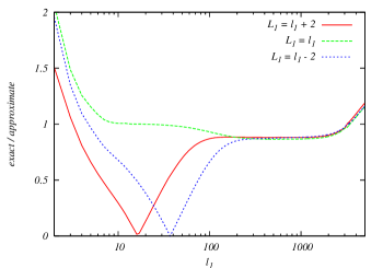
Figure 1: (color online). The ratio of the left-hand side (exact solution) to the right-hand side (approximate solution) in Eq. (95). The lines correspond to the case for $L_{1}=\ell_{1}+2$ (red solid line), for $L_{1}=\ell_{1}$ (green dashed line), and for $L_{1}=\ell_{1}-2$ (blue dotted line).

Using this approximation, namely $A=B=C\rightarrow\tau_{0}-\tau_{*}$ and $\int dA=\int dB=\int dC\rightarrow\tau_{*}/5$, the integrals with respect to $A,B,C,k^{\prime},p^{\prime}$ and $q^{\prime}$ are estimated as

$$\left[\prod\limits^{3}_{n=1}4\pi(-i)^{\ell_{n}}\int_{0}^{\infty}{k_{n}^{2}dk_{n}\over(2\pi)^{3}}\mathcal{T}^{(V)}_{I,\ell_{n}}(k_{n})\right]\int_{0}^{\infty}A^{2}dAj_{L_{1}}(k_{1}A)\int_{0}^{\infty}B^{2}dBj_{L^{\prime}_{1}}(k_{2}B)\int_{0}^{\infty}C^{2}dCj_{L^{\prime\prime}_{1}}(k_{3}C)$$

$$\qquad\qquad\times\int_{0}^{k_{D}}k_{1}^{\prime 2}dk_{1}^{\prime}P_{B}(k_{1}^{\prime})j_{L_{2}}(k_{1}^{\prime}A)j_{L^{\prime}_{3}}(k_{1}^{\prime}B)\int_{0}^{k_{D}}k_{2}^{\prime 2}dk_{2}^{\prime}P_{B}(k_{2}^{\prime})j_{L^{\prime}_{2}}(k_{2}^{\prime}B)j_{L^{\prime\prime}_{3}}(k_{2}^{\prime}C)$$

$$\qquad\qquad\times\int_{0}^{k_{D}}k_{3}^{\prime 2}dk_{3}^{\prime}P_{B}(k_{3}^{\prime})j_{L^{\prime\prime}_{2}}(k_{3}^{\prime}C)j_{L_{3}}(k_{3}^{\prime}A)$$

$$\qquad\simeq\left[\prod\limits^{3}_{n=1}4\pi(-i)^{\ell_{n}}\int_{0}^{\infty}{k_{n}^{2}dk_{n}\over(2\pi)^{3}}\mathcal{T}^{(V)}_{I,\ell_{n}}(k_{n})j_{\ell_{n}}(k_{n}(\tau_{0}-\tau_{*}))\right]$$

$$\qquad\qquad\qquad\times A_{B}^{3}(\tau_{0}-\tau_{*})^{6}\left(\frac{\tau_{*}}{5}\right)^{3}\mathcal{K}_{L_{2}L^{\prime}_{3}}^{-(n_{B}+1)}(\tau_{0}-\tau_{*})\mathcal{K}_{L^{\prime}_{2}L^{\prime\prime}_{3}}^{-(n_{B}+1)}(\tau_{0}-\tau_{*})\mathcal{K}_{L^{\prime\prime}_{2}L_{3}}^{-(n_{B}+1)}(\tau_{0}-\tau_{*})~{}.$$ (96)

Here the function ${\cal K}^{N}_{ll^{\prime}}$ is defined as

$$\mathcal{K}_{ll^{\prime}}^{N}(y) \equiv \int_{0}^{\infty}dkk^{1-N}j_{l}(ky)j_{l^{\prime}}(ky)$$ (97)

$$= \frac{\pi}{2y}\frac{y^{N-1}}{2^{N}}\frac{\Gamma(N)\Gamma(\frac{l+l^{\prime}+2-N}{2})}{\Gamma(\frac{l-l^{\prime}+1+N}{2})\Gamma(\frac{-l+l^{\prime}+1+N}{2})\Gamma(\frac{l+l^{\prime}+2+N}{2})}\ ({\rm for}\ y,N,l+l^{\prime}+2-N>0)~{},$$

which behaves asymptotically as ${\cal K}_{ll^{\prime}}^{N}(y)\propto l^{-N}$ for $l\sim l^{\prime}\gg 1$. Here we have evaluated the $k^{\prime}$ integrals by setting $k_{D}\rightarrow\infty$. This is also a good approximation because the integrands are suppressed enough for $k^{\prime},p^{\prime},q^{\prime}<k_{D}\sim{\cal O}(10)\rm Mpc^{-1}$.

III.3 Selection rules of the Wigner-$3j$ symbol

Next we consider performing the summations with respect to the helicities of vector modes. By considering the selection rules of the Wigner-$3j$ symbol, the summations over $S$, $S^{\prime}$ and $S^{\prime\prime}$ (red part in Eq. (94)) are performed as

$$\sum_{S,S^{\prime},S^{\prime\prime}=\pm 1}(-1)^{L_{2}+L^{\prime}_{2}+L^{\prime\prime}_{2}+L_{3}+L^{\prime}_{3}+L^{\prime\prime}_{3}}I^{0S-S}_{L^{\prime}_{3}1L}I^{0S-S}_{L_{2}1L}I^{0S^{\prime}-S^{\prime}}_{L^{\prime\prime}_{3}1L^{\prime}}I^{0S^{\prime}-S^{\prime}}_{L^{\prime}_{2}1L^{\prime}}I^{0S^{\prime\prime}-S^{\prime\prime}}_{L_{3}1L^{\prime\prime}}I^{0S^{\prime\prime}-S^{\prime\prime}}_{L^{\prime\prime}_{2}1L^{\prime\prime}}$$

$$\qquad\quad=\begin{cases}8I_{L^{\prime}_{3}1L}^{01-1}I_{L_{2}1L}^{01-1}I_{L^{\prime\prime}_{3}1L^{\prime}}^{01-1}I_{L^{\prime}_{2}1L^{\prime}}^{01-1}I_{L_{3}1L^{\prime\prime}}^{01-1}I_{L^{\prime\prime}_{2}1L^{\prime\prime}}^{01-1}&{\rm for\ }L_{3}^{\prime}+L_{2},L_{3}^{\prime\prime}+L_{2}^{\prime},L_{3}+L_{2}^{\prime\prime}={\rm even}\\ 0&{\rm otherwise}\end{cases}~{}.$$ (98)

By the same token, the summations over $\lambda_{1},\lambda_{2}$ and $\lambda_{3}$ (green part in Eq. (94)) are given by

$$\sum_{\lambda_{1},\lambda_{2},\lambda_{3}=\pm 1}I^{0\lambda_{1}-\lambda_{1}}_{L_{1}\ell_{1}2}I^{0\lambda_{2}-\lambda_{2}}_{L^{\prime}_{1}\ell_{2}2}I^{0\lambda_{3}-\lambda_{3}}_{L^{\prime\prime}_{1}\ell_{3}2}=\begin{cases}8I_{L_{1}\ell_{1}2}^{01-1}I_{L_{1}^{\prime}\ell_{2}2}^{01-1}I_{L_{1}^{\prime\prime}\ell_{3}2}^{01-1}&{\rm for\ }L_{1}+\ell_{1},L_{1}^{\prime}+\ell_{2},L_{1}^{\prime\prime}+\ell_{3}={\rm even}\\ 0&{\rm otherwise}\end{cases}~{}.$$ (99)

Then, using the function ${\cal K}^{N}_{ll^{\prime}}$ and the above equations, the CMB bispectrum of Eq. (17) can be written as

$$B^{(VVV)}_{III,\ell_{1}\ell_{2}\ell_{3}} \simeq \left(-\frac{32(2\pi)^{1/2}}{3\rho_{\gamma,0}}\right)^{3}\left[\prod\limits^{3}_{n=1}4\pi\int_{0}^{\infty}{k_{n}^{2}dk_{n}\over(2\pi)^{3}}\mathcal{T}^{(V)}_{I,\ell_{n}}(k_{n})j_{\ell_{n}}(k_{n}(\tau_{0}-\tau_{*}))\right]$$ (112)

$$\times\sum_{L_{1}L_{1}^{\prime}L_{1}^{\prime\prime}}I_{L_{1}\ell_{1}2}^{01-1}I_{L_{1}^{\prime}\ell_{2}2}^{01-1}I_{L_{1}^{\prime\prime}\ell_{3}2}^{01-1}\sum_{LL^{\prime}L^{\prime\prime}}\left\{\begin{array}[]{ccc}\ell_{1}&\ell_{2}&\ell_{3}\\ L^{\prime}&L^{\prime\prime}&L\end{array}\right\}$$

$$\times\sum_{\begin{subarray}{c}L_{2}L^{\prime}_{2}L^{\prime\prime}_{2}\\ L^{\prime}_{3}L^{\prime\prime}_{3}L_{3}\end{subarray}}A_{B}^{3}(\tau_{0}-\tau_{*})^{6}\left({\tau_{*}\over 5}\right)^{3}\mathcal{K}_{L_{2}L^{\prime}_{3}}^{-(n_{B}+1)}(\tau_{0}-\tau_{*})\mathcal{K}_{L^{\prime}_{2}L^{\prime\prime}_{3}}^{-(n_{B}+1)}(\tau_{0}-\tau_{*})\mathcal{K}_{L^{\prime\prime}_{2}L_{3}}^{-(n_{B}+1)}(\tau_{0}-\tau_{*})$$

$$\times(-1)^{\sum_{i=1}^{3}\frac{\ell_{i}+L_{i}+L^{\prime}_{i}+L^{\prime\prime}_{i}}{2}}I^{0~{}0~{}0}_{L_{1}L_{2}L_{3}}I^{0~{}0~{}0}_{L^{\prime}_{1}L^{\prime}_{2}L^{\prime}_{3}}I^{0~{}0~{}0}_{L^{\prime\prime}_{1}L^{\prime\prime}_{2}L^{\prime\prime}_{3}}I_{L^{\prime}_{3}1L}^{01-1}I_{L_{2}1L}^{01-1}I_{L^{\prime\prime}_{3}1L^{\prime}}^{01-1}I_{L^{\prime}_{2}1L^{\prime}}^{01-1}I_{L_{3}1L^{\prime\prime}}^{01-1}I_{L^{\prime\prime}_{2}1L^{\prime\prime}}^{01-1}$$

$$\times\left\{\begin{array}[]{ccc}L^{\prime\prime}&L&\ell_{1}\\ L_{3}&L_{2}&L_{1}\\ 1&1&2\end{array}\right\}\left\{\begin{array}[]{ccc}L&L^{\prime}&\ell_{2}\\ L^{\prime}_{3}&L^{\prime}_{2}&L^{\prime}_{1}\\ 1&1&2\end{array}\right\}\left\{\begin{array}[]{ccc}L^{\prime}&L^{\prime\prime}&\ell_{3}\\ L^{\prime\prime}_{3}&L^{\prime\prime}_{2}&L^{\prime\prime}_{1}\\ 1&1&2\end{array}\right\}~{}.$$

Here from the selection rules of the Wigner symbols Shiraishi et al. (2011), we can further limit the summation range of the multipoles as

$$\begin{split}&|\ell_{1}-\ell_{2}|\leq\ell_{3}\leq\ell_{1}+\ell_{2}~{},\\ &L_{1}=|\ell_{1}\pm 2|,~{}\ell_{1}~{},\ \ L^{\prime}_{1}=|\ell_{2}\pm 2|,~{}\ell_{2}~{},\ \ L^{\prime\prime}_{1}=|\ell_{3}\pm 2|,~{}\ell_{3}~{},\\ &|L-\ell_{2}|\leq L^{\prime}\leq L+\ell_{2}~{},\ \ {\rm Max}[|L-\ell_{1}|,|L^{\prime}-\ell_{3}|]\leq L^{\prime\prime}\leq{\rm Min}[L+\ell_{1},L^{\prime}+\ell_{3}]~{},\\ &(L_{2},L^{\prime}_{3})=(|L-1|,|L\pm 1|),~{}(L,L),~{}(L+1,|L\pm 1|)~{},\\ &(L^{\prime}_{2},L^{\prime\prime}_{3})=(|L^{\prime}-1|,|L^{\prime}\pm 1|),~{}(L^{\prime},L^{\prime}),~{}(L^{\prime}+1,|L^{\prime}\pm 1|)~{},\\ &(L^{\prime\prime}_{2},L_{3})=(|L^{\prime\prime}-1|,|L^{\prime\prime}\pm 1|),~{}(L^{\prime\prime},L^{\prime\prime}),~{}(L^{\prime\prime}+1,|L^{\prime\prime}\pm 1|)~{},\\ &L_{1}+L_{2}+L_{3}={\rm even}~{},\ \ L^{\prime}_{1}+L^{\prime}_{2}+L^{\prime}_{3}={\rm even}~{},\ \ L^{\prime\prime}_{1}+L^{\prime\prime}_{2}+L^{\prime\prime}_{3}={\rm even}~{},\\ &|L_{1}-L_{2}|\leq L_{3}\leq L_{1}+L_{2}~{},\ \ |L^{\prime}_{1}-L^{\prime}_{2}|\leq L^{\prime}_{3}\leq L^{\prime}_{1}+L^{\prime}_{2}~{},\ \ |L^{\prime\prime}_{1}-L^{\prime\prime}_{2}|\leq L^{\prime\prime}_{3}\leq L^{\prime\prime}_{1}+L^{\prime\prime}_{2}~{}.\end{split}$$ (113)

and from the above restrictions the multipoles in the bispectrum, $\ell_{1},\ell_{2}$ and $\ell_{3}$, are also limited as

$$\begin{split}&\ell_{1}+\ell_{2}+\ell_{3}={\rm even}~{}.\end{split}$$ (114)

Therefore, these selection rules significantly reduce the number of calculation. In these ranges, while $L^{\prime}$ and $L^{\prime\prime}$ are limited by $L$, only $L$ has no upper bound. However, we can show that the summation of $L$ is suppressed at $\ell_{1}\sim\ell_{2}\sim\ell_{3}\ll L$ as follows. When the summations with respect to $L,L^{\prime}$ and $L^{\prime\prime}$ are evaluated at large $L,L^{\prime}$ and $L^{\prime\prime}$, namely $\ell_{1},\ell_{2},\ell_{3}\ll L\sim L^{\prime}\sim L^{\prime\prime},L_{2}\sim L^{\prime}_{3}\sim L,L^{\prime}_{2}\sim L^{\prime\prime}_{3}\sim L^{\prime}$ and $L^{\prime\prime}_{2}\sim L_{3}\sim L^{\prime\prime}$, we get

$$\sum_{LL^{\prime}L^{\prime\prime}}\left\{\begin{array}[]{ccc}\ell_{1}&\ell_{2}&\ell_{3}\\ L^{\prime}&L^{\prime\prime}&L\end{array}\right\}\sum_{\begin{subarray}{c}L_{2}L^{\prime}_{2}L^{\prime\prime}_{2}\\ L^{\prime}_{3}L^{\prime\prime}_{3}L_{3}\end{subarray}}\mathcal{K}_{L_{2}L^{\prime}_{3}}^{-(n_{B}+1)}(\tau_{0}-\tau_{*})\mathcal{K}_{L^{\prime}_{2}L^{\prime\prime}_{3}}^{-(n_{B}+1)}(\tau_{0}-\tau_{*})\mathcal{K}_{L^{\prime\prime}_{2}L_{3}}^{-(n_{B}+1)}(\tau_{0}-\tau_{*})$$ (117)

$$\qquad\qquad\times(-1)^{\sum_{i=1}^{3}\frac{L_{i}+L_{i}^{\prime}+L^{\prime\prime}_{i}}{2}}I^{0~{}0~{}0}_{L_{1}L_{2}L_{3}}I^{0~{}0~{}0}_{L^{\prime}_{1}L^{\prime}_{2}L^{\prime}_{3}}I^{0~{}0~{}0}_{L^{\prime\prime}_{1}L^{\prime\prime}_{2}L^{\prime\prime}_{3}}I_{L^{\prime}_{3}1L}^{01-1}I_{L_{2}1L}^{01-1}I_{L^{\prime\prime}_{3}1L^{\prime}}^{01-1}I_{L^{\prime}_{2}1L^{\prime}}^{01-1}I_{L_{3}1L^{\prime\prime}}^{01-1}I_{L^{\prime\prime}_{2}1L^{\prime\prime}}^{01-1}$$

$$\qquad\qquad\times\left\{\begin{array}[]{ccc}L^{\prime\prime}&L&\ell_{1}\\ L_{3}&L_{2}&L_{1}\\ 1&1&2\end{array}\right\}\left\{\begin{array}[]{ccc}L&L^{\prime}&\ell_{2}\\ L^{\prime}_{3}&L^{\prime}_{2}&L^{\prime}_{1}\\ 1&1&2\end{array}\right\}\left\{\begin{array}[]{ccc}L^{\prime}&L^{\prime\prime}&\ell_{3}\\ L^{\prime\prime}_{3}&L^{\prime\prime}_{2}&L^{\prime\prime}_{1}\\ 1&1&2\end{array}\right\}$$ (127)

$$\qquad\propto\sum_{LL^{\prime}L^{\prime\prime}}(LL^{\prime}L^{\prime\prime})^{n_{B}+4/3}~{}.$$ (128)

Therefore, we may obtain a stable result with the summations over a limited number of $L$ when we consider the magnetic power spectrum is as red as $n_{B}\sim-2.9$, because the summations of $L^{\prime}$ and $L^{\prime\prime}$ are limited by $L$. Here, we use the analytic formulas of the $I$ symbols which are given by

$$\left\{\begin{array}[]{ccc}\ell_{1}&\ell_{2}&\ell_{3}\\ L^{\prime}&L^{\prime\prime}&L\end{array}\right\}\propto(LL^{\prime}L^{\prime\prime})^{-1/6}~{},\ \ {\cal K}_{L_{2}L^{\prime}_{3}}^{-(n_{B}+1)}\propto L^{n_{B}+1}~{},\ \ \left\{\begin{array}[]{ccc}L^{\prime\prime}&L&\ell_{1}\\ L_{3}&L_{2}&L_{1}\\ 1&1&2\end{array}\right\}\propto(L^{\prime\prime}L)^{-1/2}~{},$$ (134)

as described in detail in Appendix B.

Using the approximation and the summation rules described above, we can perform the computation of the CMB bispectrum containing full-angular dependence in a reasonable time.

IV Results

Now we show the result of the CMB temperature bispectrum induced from the vector anisotropic stress $\Pi_{Bv}^{(\lambda)}$. In order to compute numerically, we insert Eq. (112) into the Boltzmann code for anisotropies in the microwave background (CAMB) Lewis (2004a); Lewis et al. (2000). We use the transfer function of magnetic-compensated modes calculated as Refs. Shaw and Lewis (2010); Lewis (2004b), which is shown in Appendix A. In the calculation of the Wigner-$3j,6j$ and 9j symbols, we use a common mathematical library called SLATEC sla and analytical expressions in Appendix B.

In Fig. 2, we show the reduced bispectra of the temperature fluctuation induced by the PMFs defined as Komatsu and Spergel (2001)

$$b^{(VVV)}_{III,\ell_{1}\ell_{2}\ell_{3}}\equiv\left(I^{0~{}0~{}0}_{\ell_{1}\ell_{2}\ell_{3}}\right)^{-1}B^{(VVV)}_{III,\ell_{1}\ell_{2}\ell_{3}}~{},$$ (135)

for $\ell_{1}=\ell_{2}=\ell_{3}$. Red solid and green dashed lines correspond to the bispectrum given by Eq. (112) with the spectral index of the power spectrum of PMFs fixed as $n_{B}=-2.9$ and $-2.8$, respectively. One can see that the peak of each bispectrum is located at $\ell\sim 1500$ and the position is similar to that of the angular power spectrum $C^{(V)}_{I,\ell}$ induced from the vector mode as calculated in Appendix C. At small scales, the vector mode contributes to the CMB power spectrum through the Doppler effect. Thus we can easily find that through this Doppler effect the vector mode can also enhance the CMB bispectrum. In our related paper Shiraishi et al. (2010a), we have also shown that the contribution from the vector mode dominates over that from the scalar mode at the scales around $\ell\sim 1500$ in the CMB bispectrum induced from the PMFs, as in the CMB power spectrum.

As for the amplitude of the CMB bispectrum of the vector mode induced from the PMFs, one can expect $b_{III,\ell\ell\ell}^{(VVV)}\sim C_{I,\ell}^{(V)3/2}$ by using the amplitude of the CMB power spectrum of the vector mode induced from the PMFs. However, in Fig. 2 we find that the amplitude of $b_{III,\ell\ell\ell}^{(VVV)}$ is smaller than the above expectation. This is because the configuration of multipoles, corresponding to the angles of wave number vectors, is limited to the conditions placed by the Wigner symbols.

We can understand this by considering the scaling relation with respect to $\ell$. If the magnetic power spectrum given by Eq. (4) is close to the scale-invariant shape, the configuration that satisfies $L\sim L^{\prime\prime}\sim\ell$ and $L^{\prime}\sim 1$ contributes dominantly in the summations. Furthermore, the other multipoles are evaluated as

$$L_{1}\sim L^{\prime}_{1}\sim L^{\prime\prime}_{1}\sim\ell~{},\ \ L_{2}\sim L^{\prime\prime}_{2}\sim L_{3}\sim L^{\prime}_{3}\sim\ell~{},\ \ L^{\prime}_{2}\sim L^{\prime\prime}_{3}\sim 1~{},$$ (136)

from the triangle conditions described in Appendix B. Then we can find $b^{(VVV)}_{III,\ell\ell\ell}\propto\ell^{2n_{B}+4}$ for $\ell\lesssim 1000$, where we have also used the following relations

$$\begin{split}&\int k^{2}dk\mathcal{T}^{(V)}_{I,\ell_{i}}(k)j_{\ell_{i}}(k(\tau_{0}-\tau_{*}))\propto\ell~{},\ \ \left\{\begin{array}[]{ccc}\ell_{1}&\ell_{2}&\ell_{3}\\ L^{\prime}&L^{\prime\prime}&L\end{array}\right\}\propto\ell^{-1}~{},\ \ {\cal K}_{L_{2}L^{\prime}_{3}}^{-(n_{B}+1)}\sim{\cal K}_{L^{\prime\prime}_{2}L_{3}}^{-(n_{B}+1)}\propto\ell^{n_{B}+1}~{},\\ &\left\{\begin{array}[]{ccc}L^{\prime\prime}&L&\ell_{1}\\ L_{3}&L_{2}&L_{1}\\ 1&1&2\end{array}\right\}\propto\ell^{-3/2}~{},\ \ \left\{\begin{array}[]{ccc}L&L^{\prime}&\ell_{1}\\ L^{\prime}_{3}&L^{\prime}_{2}&L_{1}^{\prime}\\ 1&1&2\end{array}\right\}\sim\left\{\begin{array}[]{ccc}L^{\prime}&L^{\prime\prime}&\ell_{1}\\ L^{\prime\prime}_{3}&L^{\prime\prime}_{2}&L^{\prime\prime}_{1}\\ 1&1&2\end{array}\right\}\propto\ell^{-1}~{},\end{split}$$ (137)

which, except for the first relation, are also coming from the triangle conditions of the Wigner $3$-j symbols. Therefore, combining with the scaling relation of the CMB power spectrum mentioned in Appendix C, we find that $b^{(VVV)}_{III,\ell\ell\ell}$ is suppressed by a factor $\ell^{(n_{B}-1)/2}$ from $C^{(V)3/2}_{I,\ell}$. This is the reason why our constraint on the PMF from the vector bispectrum is not so much stronger than expected from the scalar counterpart.

From this figure, we also find that the CMB bispectrum becomes steeper if $n_{B}$ becomes larger, which is similar to the case of the power spectrum. This will lead to another constraint on the strength of the PMFs. In particular, as shown in Refs. Shiraishi et al. (2010a); Brown and Crittenden (2005); Seshadri and Subramanian (2009); Caprini et al. (2009); Cai et al. (2010); Trivedi et al. (2010), although the CMB bispectrum induced from the PMFs is dominated by the contribution from the scalar mode on large scales, such contribution becomes small on small scales. Therefore, it will be important to consider not only the contribution from the scalar mode induced from the PMFs on large scales but also that from the vector mode on small scales to obtain the constraint on the amplitude and the spectral index of the PMFs’ power spectrum simultaneously.

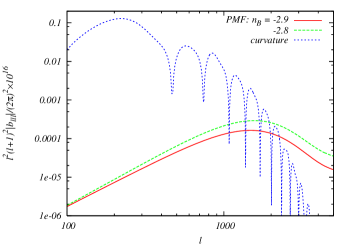
Figure 2: (color online). Absolute values of the normalized reduced bispectra of temperature fluctuation for a configuration $\ell_{1}=\ell_{2}=\ell_{3}$. The lines correspond to the spectra generated from vector anisotropic stress for $n_{B}=-2.9$ (red solid line) and $-2.8$ (green dashed line), and primordial non-Gaussianity with $f^{\rm local}_{\rm NL}=5$ (blue dotted line). The strength of PMFs is fixed to $B_{1{\rm Mpc}}=4.7{\rm nG}$ and the other cosmological parameters are fixed to the mean values limited from WMAP-7yr data reported in Ref. Komatsu et al. (2010).

In Fig. 3, we show the reduced bispectrum $b_{III,\ell_{1}\ell_{2}\ell_{3}}$ with respect to $\ell_{3}$ with setting $\ell_{1}=\ell_{2}$. From this figure we can see that the normalized reduced bispectrum of the vector mode induced from the PMFs for $\ell_{1},\ell_{2},\ell_{3}\gtrsim 100$ is nearly flat and given as

$$\ell_{1}(\ell_{1}+1)\ell_{3}(\ell_{3}+1)|b^{(VVV)}_{III,\ell_{1}\ell_{2}\ell_{3}}|\sim 2\times 10^{-19}\left(\frac{B_{1\rm Mpc}}{4.7\rm nG}\right)^{6}.$$

(138)

It is seen that $b^{(VVV)}_{III,\ell_{1}\ell_{2}\ell_{3}}$ for $n_{B}\simeq-3$ dominates in $\ell_{1}=\ell_{2}\gg\ell_{3}$. This means that the shape of the CMB bispectrum generated from the vector anisotropic stress of the PMF is close to the so-called local-type configuration if the power spectrum of the PMF is nearly scale invariant. We can understand this by the analytical evaluation as follows. As mentioned above, in the summations of Eq. (112), the configuration that $L\sim\ell_{1},L^{\prime}\sim 1$ and $L^{\prime\prime}\sim\ell_{3}$ contributes dominantly. By using this and the approximations that

$$L_{1}\sim\ell_{1}~{},\ \ L^{\prime}_{1}\sim\ell_{2}~{},\ \ L^{\prime\prime}_{1}\sim\ell_{3}~{},\ \ L_{2}\sim L^{\prime}_{3}\sim L~{},\ \ L^{\prime}_{2}\sim L^{\prime\prime}_{3}\sim L^{\prime}~{},\ \ L^{\prime\prime}_{2}\sim L_{3}\sim L^{\prime\prime}~{},$$ (139)

which again come from the triangle conditions from the Wigner symbols, the scaling relation of $\ell_{3}$ at large scale is evaluated as $b^{(VVV)}_{III,\ell_{1}\ell_{2}\ell_{3}}\propto\ell_{3}^{n_{B}+1}$. From this estimation we can find that $\ell_{1}(\ell_{1}+1)\ell_{3}(\ell_{3}+1)b^{(VVV)}_{III,\ell_{1}\ell_{2}\ell_{3}}\propto\ell_{3}^{0.1}$, for $n_{B}=-2.9$, and $\ell_{3}^{0.2}$ for $n_{B}=-2.8$, respectively, which match the behaviors of the bispectra in Fig.  3.

In order to obtain a valid constraint on the magnitude of the PMF, we compare the bispectrum induced from the PMF with that from the local-type primordial non-Gaussianity in the curvature perturbations, which is typically estimated as Riotto (2008)

$$\ell_{1}(\ell_{1}+1)\ell_{3}(\ell_{3}+1)b_{\ell_{1}\ell_{2}\ell_{3}}\sim 4\times 10^{-18}f^{\rm local}_{\rm NL}~{}.$$ (140)

By comparing this with Eq. (138), the relation between the magnitudes of the PMF with the nearly scale-invariant power spectrum and $f^{\rm local}_{\rm NL}$ is derived as

$$\left(\frac{B_{1\rm Mpc}}{1\rm nG}\right)\sim 7.74~{}|f^{{\rm local}}_{\rm NL}|^{1/6}\ \ ({\rm for~{}n_{B}\sim-3})~{}.$$ (141)

By making use of the above relation, we can place the upper bound of strength of the PMF. If we assume $|f^{\rm local}_{\rm NL}|<100$ as considered in Ref. Seshadri and Subramanian (2009), we can translate this to the constraint on the PMF amplitude as $B_{1\rm Mpc}<17{\rm nG}$, which is stronger by a factor of 2 than estimated in Ref. Seshadri and Subramanian (2009). On the other hand, from the current observational lower bound from WMAP 7-yr data mentioned in Sec. I, namely $f_{\rm NL}^{\rm local}>-10$, we derive $B_{1\rm Mpc}<11{\rm nG}$. If we use $|f_{\rm NL}^{\rm local}|<5$ which is expected from Planck experiment [Planck Collaboration] (2006), we will meet a tight constraint as $B_{1\rm Mpc}<10{\rm nG}$.

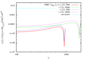
Figure 3: (color online). Absolute values of the normalized reduced bispectra of temperature fluctuation given by Eq. (112) and generated by primordial non-Gaussianity given by Eq. (140) as a function of $\ell_{3}$ with $\ell_{1}$ and $\ell_{2}$ fixed to some value as indicated. Each parameter is fixed to the same value defined in Fig. 2.

V Summary and Discussion

In this paper, we present a calculation method of the bispectrum of CMB temperature fluctuation induced from the vector mode of the PMFs as described in Ref. Shiraishi et al. (2010b), by taking into account the full angular dependence of the bispectrum of magnetic fields. We expand all the angular dependence with the spin spherical harmonics and convert them to the summations of the Wigner symbols. In the radial integrals and timelike integrals, we use only one approximation that the interval of the timelike integrals is confined to the moment of the recombination, which corresponds to neglecting the vector mode ISW effect. This approximation is valid because the radiation transfer function of the vector magnetic mode has a sharp peak around $k\sim\ell/(\tau_{0}-\tau_{*})$ which comes from the Doppler effect of the baryon vorticity induced from the magnetic field. We checked that the errors by the approximation are less than $10\%$.

As the results, it is found that the CMB bispectrum from the magnetic vector mode dominates at small scales compared to that from the magnetic scalar mode which has been calculated in the literature. It is also found that the bispectrum has significant signals on the squeezed limit, namely the local-type configuration, if the magnetic field power spectrum is nearly scale invariant. This is understood by considering the asymptotic scaling relation of the CMB bispectrum. We also investigate the dependence of the spectral index of the power spectrum of the PMFs on the CMB bispectrum and we find that the CMB bispectrum of the vector mode induced from the PMFs is more sensitive to the spectral index of the PMFs’ power spectrum than that of the scalar mode. Hence, we conclude that it is important to consider not only the contribution from the scalar mode of the PMFs on large scales, but also that from the vector mode on small scales to obtain the constraint on the amplitude and the spectral index of the PMFs’ power spectrum simultaneously.

By translating the current bound on the local-type non-Gaussianity from the CMB bispectrum into the bound on the amplitude of the magnetic fields, we obtain a new limit: $B_{1\rm Mpc}<11{\rm nG}$. This is a rough estimate and a tighter constraint is expected if one considers the full $\ell$ contribution by using an appropriate estimator of the CMB bispectrum induced from the primordial magnetic fields.

Because of the complicated discussions and mathematical manipulations, here we restrict our attention to the temperature bispectrum from the vector mode of the PMFs. However, one will be able to apply this methodology to the bispectra of CMB temperature and polarization from the scalar, vector and tensor modes.

Appendix A CMB temperature fluctuations induced from vector anisotropic stresses

In Refs. Mack et al. (2002); Kahniashvili and Lavrelashvili (2010), it is discussed that the temperature fluctuations are generated via Doppler and integrated Sachs-Wolfe effects on the CMB vector modes. Based on them, we derive the transfer function of the vector magnetic mode as follows.

When we decompose the metric perturbations into vector components as

$$\delta g_{0c} = \delta g_{c0}=a^{2}A_{c}~{},$$ (142)

$$\delta g_{cd} = a^{2}(\partial_{c}h^{(V)}_{d}+\partial_{d}h^{(V)}_{c})~{},$$ (143)

we can construct two gauge-invariant variables, namely a vector perturbation of the extrinsic curvature and a vorticity, as

$${\bf V} \equiv {\bf A}-{\bf h}^{\prime}~{},$$ (144)

$${\bf\Omega} \equiv {\bf v}-{\bf A}~{},$$ (145)

where ${\bf v}$ is the spatial part of the four-velocity perturbation of a stationary fluid element and a dash denotes a partial derivative of the conformal time $\tau$. Here, choosing a gauge as ${\bf h}^{\prime}=0$, we can express the Einstein equation

$${\bf V}^{\prime}+2\frac{a^{\prime}}{a}{\bf V}=-\frac{16\pi G\rho_{\gamma,0}({\bf\Pi_{\gamma}^{(V)}}+{\bf\Pi_{\nu}^{(V)}}+{\bf\Pi_{B}^{(V)}})}{a^{2}k}~{},$$ (146)

and the Euler equations for photons and baryons

$${\bf\Omega_{\gamma}}^{\prime}+\tau_{c}^{\prime}({\bf v_{\gamma}}-{\bf v_{b}}) = 0~{},$$ (147)

$${\bf\Omega_{b}}^{\prime}+\frac{a^{\prime}}{a}{\bf\Omega_{b}}-\frac{\tau_{c}^{\prime}}{R}({\bf v_{\gamma}}-{\bf v_{b}}) = \frac{k\rho_{\gamma,0}{\bf\Pi_{B}^{(V)}}}{a^{4}(\rho_{b}+p_{b})}~{}.$$ (148)

Here $\Pi^{(V)}_{a}=-i\hat{k}_{b}P_{ac}\Pi_{bc}$, $p$ is the isotropic pressure, the indices $\gamma,\nu$ and $b$ denote the photon, neutrino and baryon, $\tau_{c}$ is the optical depth, and $R\equiv(\rho_{b}+p_{b})/(\rho_{\gamma}+p_{\gamma})$. In the tight-coupling limit as ${\bf v_{\gamma}}\simeq{\bf v_{b}}$, the photon vorticity is comparable to the baryon one: ${\bf\Omega_{\gamma}}\simeq{\bf\Omega_{b}}\equiv{\bf\Omega}$. Then, the Euler equations (147) and (148) are combined into

$$(1+R){\bf\Omega}^{\prime}+R\frac{a^{\prime}}{a}{\bf\Omega}=\frac{k\rho_{\gamma,0}{\bf\Pi_{B}^{(V)}}}{a^{4}(\rho_{\gamma}+p_{\gamma})}~{},$$ (149)

and this solution is given by

$${\bf\Omega}({\bf k},\tau) \simeq \beta(k,\tau){\bf\Pi_{B}^{(V)}(k)}~{},$$ (150)

$$\beta(k,\tau) = \begin{cases}\frac{k\tau\rho_{\gamma,0}}{(1+R)(\rho_{\gamma,0}+p_{\gamma,0})}&{\rm for}\ k<k_{S}\\ \frac{5\tau_{c}^{\prime}\rho_{\gamma,0}}{k(\rho_{\gamma,0}+p_{\gamma,0})}&{\rm for}\ k>k_{S}\end{cases}~{},$$ (151)

where $k_{S}$ means the Silk damping scale.

As mentioned above, the CMB temperature anisotropies of vector modes are produced through Doppler and integrated Sachs-Wolfe effect as

$$\frac{\Delta T(\hat{\bf n})}{T} = -{\bf v_{\gamma}}\cdot\hat{\bf n}|^{\tau_{0}}_{\tau_{*}}+\int_{\tau_{*}}^{\tau_{0}}d\tau{\bf V}^{\prime}\cdot\hat{\bf n}~{},$$ (152)

where $\tau_{0}$ is today and $\tau_{*}$ is the recombination epoch in conformal time, $\mu_{k,n}\equiv\hat{\bf k}\cdot\hat{\bf n}$, $x\equiv k(\tau_{0}-\tau)$, and $\hat{\bf n}$ is an unit vector along the line-of-sight direction. Because of compensation of the anisotropic stresses, a solution of the Einstein equation (146) expresses the decaying signature as ${\bf V}\propto a^{-2}$ after neutrino decoupling. Therefore, in an integrated Sachs-Wolfe effect term, the contribution around the recombination epoch is dominant. Furthermore, neglecting dipole contribution due to ${\bf v}$ today, we can form the coefficient of anisotropies as

$$a_{\ell m} \equiv \int d^{2}\hat{\bf n}\frac{\Delta T(\hat{\bf n})}{T}Y^{*}_{\ell m}(\hat{\bf n})$$

$$\simeq \int\frac{d^{3}{\bf k}}{(2\pi)^{3}}\int d^{2}\hat{\bf n}[{\bf\Pi_{B}^{(V)}}({\bf k})\cdot\hat{\bf n}]Y^{*}_{\ell m}(\hat{\bf n})\beta(k,\tau_{*})e^{-i\mu_{k,n}x_{*}}~{}.$$

In the transformation $\hat{\bf n}\rightarrow(\mu_{k,n},\phi_{k,n})$, the functions are rewritten as

$${\bf\Pi_{B}^{(V)}(\bf k)}\cdot\hat{\bf n} \rightarrow -i\sqrt{\frac{1-\mu_{k,n}^{2}}{2}}\sum_{\lambda=\pm 1}\Pi^{(\lambda)}_{Bv}({\bf k})e^{i\lambda\phi_{k,n}}~{},$$ (153)

$$Y^{*}_{\ell m}(\hat{\bf n}) \rightarrow \sum_{m^{\prime}}D^{(\ell)}_{mm^{\prime}}\left(S(\hat{\bf k})\right)Y^{*}_{\ell m^{\prime}}(\Omega_{k,n})~{},$$ (154)

$$d^{2}\hat{\bf n} \rightarrow d\Omega_{k,n}~{},$$ (155)

where we use the relation: $\displaystyle\Pi^{(V)}_{a}=\sum_{\lambda=\pm 1}-i\Pi_{Bv}^{(\lambda)}\epsilon_{a}^{(\lambda)}$ and the Wigner $D$ matrix under the rotational transformation of an unit vector parallel to $z$ axis into $\hat{\bf k}$ corresponding to Eq. (A7) of Ref. Shiraishi et al. (2010b). Therefore, performing the integration over $\Omega_{k,n}$ in the same manner as Ref. Shiraishi et al. (2010b) , we can obtain the explicit form of $a_{\ell m}$ and express the radiation transfer function introduced in Eq. (15) as

$${\cal T}^{(V)}_{I,\ell}(k)\simeq\left[\frac{(\ell+1)!}{(\ell-1)!}\right]^{1/2}\frac{\beta(k,\tau_{*})}{\sqrt{2}}\frac{j_{\ell}(x_{*})}{x_{*}}~{}.$$ (156)

This is consistent with the results presented in Refs. Lewis (2004a, b).

Appendix B Analytic expressions of the Wigner symbols

The Wigner-$3j,6j$ and $9j$ symbols express Clebsch-Gordan coefficients between two other eigenstates coupled to two three, and four individual momenta Hu (2001); Gurau (2008); Jahn and Hope (1954). Their selection rules and several properties are reviewed in Ref. mat ; Shiraishi et al. (2011). Here, using their knowledge, we show the analytical formulas of the Wigner symbols which appear in the CMB bispectrum of Eq. (112).

The $I$ symbols, which are defined as $I^{s_{1}s_{2}s_{3}}_{l_{1}l_{2}l_{3}}\equiv\sqrt{\frac{(2l_{1}+1)(2l_{2}+1)(2l_{3}+1)}{4\pi}}\left(\begin{array}[]{ccc}l_{1}&l_{2}&l_{3}\\ s_{1}&s_{2}&s_{3}\end{array}\right)$, are expressed as

$$I_{l_{1}l_{2}l_{3}}^{0~{}0~{}0} = \sqrt{\frac{\prod_{i=1}^{3}(2l_{i}+1)}{4\pi}}(-1)^{\sum_{i=1}^{3}\frac{-l_{i}}{2}}$$ (157)

$$\times\frac{\left(\sum_{i=1}^{3}\frac{l_{i}}{2}\right)!\sqrt{(-l_{1}+l_{2}+l_{3})!}\sqrt{(l_{1}-l_{2}+l_{3})!}\sqrt{(l_{1}+l_{2}-l_{3})!}}{\left(\frac{-l_{1}+l_{2}+l_{3}}{2}\right)!\left(\frac{l_{1}-l_{2}+l_{3}}{2}\right)!\left(\frac{l_{1}+l_{2}-l_{3}}{2}\right)!\sqrt{(\sum_{i=1}^{3}l_{i}+1)!}}\ \ ({\rm for\ }l_{1}+l_{2}+l_{3}={\rm even})$$

$$= 0\ \ ({\rm for\ }l_{1}+l_{2}+l_{3}={\rm odd})~{},$$ (158)

$$I_{l_{1}~{}l_{2}~{}l_{3}}^{0~{}1~{}-1} = \sqrt{\frac{5}{8\pi}}(-1)^{l_{2}+1}\sqrt{\frac{(l_{2}-1)(l_{2}+1)}{l_{2}-1/2}}\ \ ({\rm for\ }l_{1}=l_{2}-2,l_{3}=2)$$ (159)

$$= \sqrt{\frac{15}{16\pi}}(-1)^{l_{2}}\sqrt{\frac{l_{2}+1/2}{(l_{2}-1/2)(l_{2}+3/2)}}\ \ ({\rm for\ }l_{1}=l_{2},l_{3}=2)$$ (160)

$$= \sqrt{\frac{5}{8\pi}}(-1)^{l_{2}}\sqrt{\frac{l_{2}(l_{2}+2)}{l_{2}+3/2}}\ \ ({\rm for\ }l_{1}=l_{2}+2,l_{3}=2)$$ (161)

$$= \sqrt{\frac{3}{8\pi}}(-1)^{l_{3}+1}\sqrt{l_{3}+1}\ \ ({\rm for\ }l_{1}=l_{3}-1,l_{2}=1)$$ (162)

$$= \sqrt{\frac{3}{4\pi}}(-1)^{l_{3}+1}\sqrt{l_{3}+1/2}\ \ ({\rm for\ }l_{1}=l_{3},l_{2}=1)$$ (163)

$$= \sqrt{\frac{3}{8\pi}}(-1)^{l_{3}+1}\sqrt{l_{3}}\ \ ({\rm for\ }l_{1}=l_{3}+1,l_{2}=1)~{}.$$ (164)

Three Wigner-$9j$ symbols in Eq. (112) are calculated as

$$\left\{\begin{array}[]{ccc}l_{1}&l_{2}&l_{3}\\ l_{4}&l_{5}&l_{6}\\ 1&1&2\end{array}\right\} = \sqrt{\frac{2(l_{3}\pm 1)+1}{5}}\left\{\begin{array}[]{ccc}l_{1}&l_{4}&1\\ l_{3}\pm 2&l_{3}\pm 1&l_{5}\end{array}\right\}\left\{\begin{array}[]{ccc}l_{2}&l_{5}&1\\ l_{3}\pm 1&l_{3}&l_{1}\end{array}\right\}\ \ ({\rm for\ }l_{6}=l_{3}\pm 2)$$ (172)

$$= \sqrt{\frac{(2l_{3}-1)(2l_{3}+2)(2l_{3}+3)}{30(2l_{3})(2l_{3}+1)}}\left\{\begin{array}[]{ccc}l_{1}&l_{4}&1\\ l_{3}&l_{3}-1&l_{5}\end{array}\right\}\left\{\begin{array}[]{ccc}l_{2}&l_{5}&1\\ l_{3}-1&l_{3}&l_{1}\end{array}\right\}$$ (187)

$$+\sqrt{\frac{2(2l_{3}-1)(2l_{3}+1)(2l_{3}+3)}{15(2l_{3})(2l_{3}+2)}}\left\{\begin{array}[]{ccc}l_{1}&l_{4}&1\\ l_{3}&l_{3}&l_{5}\end{array}\right\}\left\{\begin{array}[]{ccc}l_{2}&l_{5}&1\\ l_{3}&l_{3}&l_{1}\end{array}\right\}$$

$$+\sqrt{\frac{(2l_{3}-1)(2l_{3})(2l_{3}+3)}{30(2l_{3}+1)(2l_{3}+2)}}\left\{\begin{array}[]{ccc}l_{1}&l_{4}&1\\ l_{3}&l_{3}+1&l_{5}\end{array}\right\}\left\{\begin{array}[]{ccc}l_{2}&l_{5}&1\\ l_{3}+1&l_{3}&l_{1}\end{array}\right\}\ \ ({\rm for\ }l_{6}=l_{3})~{},$$

where these Wigner-$6j$ symbols are analytically given by

$$\left\{\begin{array}[]{ccc}l_{1}&l_{2}&1\\ l_{4}&l_{5}&l_{6}\end{array}\right\} = (-1)^{l_{1}+l_{4}+l_{6}+1}\sqrt{\frac{{}_{l_{1}+l_{4}+l_{6}+2}P_{2}~{}{}_{l_{1}+l_{4}-l_{6}+1}P_{2}}{{}_{2l_{4}+3}P_{3}~{}{}_{2l_{1}+1}P_{3}}}\ \ ({\rm for\ }l_{2}=l_{1}-1,l_{5}=l_{4}+1)$$ (191)

$$= (-1)^{l_{1}+l_{4}+l_{6}+1}\sqrt{\frac{2(l_{1}+l_{4}+l_{6}+2)(l_{1}+l_{4}-l_{6}+1)(-l_{1}+l_{4}+l_{6}+1)(l_{1}-l_{4}+l_{6})}{{}_{2l_{4}+3}P_{3}~{}{}_{2l_{1}+2}P_{3}}}$$

$$\qquad\qquad\qquad\qquad\qquad\qquad\qquad\qquad\qquad\qquad\qquad({\rm for\ }l_{2}=l_{1},l_{5}=l_{4}+1)$$

$$= (-1)^{l_{1}+l_{4}+l_{6}+1}\sqrt{\frac{{}_{-l_{1}+l_{4}+l_{6}+1}P_{2}~{}{}_{l_{1}-l_{4}+l_{6}+1}P_{2}}{{}_{2l_{4}+3}P_{3}~{}{}_{2l_{1}+3}P_{3}}}\ \ ({\rm for\ }l_{2}=l_{1}+1,l_{5}=l_{4}+1)$$ (195)

$$= (-1)^{l_{1}+l_{4}+l_{6}+1}\left[l_{4}(l_{4}+1)+l_{1}(l_{1}-1)(l_{4}+1)-l_{6}(l_{6}+1)-l_{1}(l_{1}+1)l_{4}\right]$$

$$\times\sqrt{\frac{2(l_{1}+l_{4}+l_{6}+1)(l_{1}+l_{4}-l_{6})}{(-l_{1}+l_{4}+l_{6}+1)(l_{1}-l_{4}+l_{6}){}_{2l_{4}+2}P_{3}~{}{}_{2l_{1}+1}P_{3}}}\ \ ({\rm for\ }l_{2}=l_{1}-1,l_{5}=l_{4})$$

$$= 2(-1)^{l_{1}+l_{4}+l_{6}+1}\frac{l_{4}(l_{4}+1)+l_{1}(l_{1}+1)(l_{4}+1)-l_{6}(l_{6}+1)-l_{1}(l_{1}+1)l_{4}}{\sqrt{{}_{2l_{4}+2}P_{3}~{}{}_{2l_{1}+2}P_{3}}}$$

$$\qquad\qquad\qquad\qquad\qquad\qquad\qquad\qquad\qquad\qquad\qquad({\rm for\ }l_{2}=l_{1},l_{5}=l_{4})$$

$$= (-1)^{l_{1}+l_{4}+l_{6}+1}\left[l_{4}(l_{4}+1)+(l_{1}+1)(l_{1}+2)(l_{4}+1)-l_{6}(l_{6}+1)-l_{1}(l_{1}+1)l_{4}\right]$$

$$\times\sqrt{\frac{2(-l_{1}+l_{4}+l_{6})(l_{1}-l_{4}+l_{6}+1)}{(l_{1}+l_{4}+l_{6}+2)(l_{1}+l_{4}-l_{6}+1){}_{2l_{4}+2}P_{3}~{}{}_{2l_{1}+3}P_{3}}}\ \ ({\rm for\ }l_{2}=l_{1}+1,l_{5}=l_{4})~{}.$$

Using these analytical formulas, one can reduce the time cost involved with calculating the bispectrum of Eq. (112).

Appendix C CMB all-sky power spectrum of vector modes generated from PMFs

In this section, we derive CMB power spectrum of vector modes sourced from PMFs in the same manner as presented previously and check the validity of our original approach.

From Eq. (15), the CMB power spectrum of the intensity mode induced from $\Pi_{Bv,\ell m}^{(\pm 1)}$ is formulated as

$$\Braket{a^{(V)}_{I,\ell_{1}m_{1}}a^{(V)*}_{I,\ell_{2}m_{2}}} = \left[\prod_{n=1}^{2}4\pi\int_{0}^{\infty}{k_{n}^{2}dk_{n}\over(2\pi)^{3}}\mathcal{T}^{(V)}_{I,\ell_{n}}(k_{n})\right](-i)^{\ell_{1}}i^{\ell_{2}}\sum\limits_{\lambda_{1},\lambda_{2}=\pm 1}\lambda_{1}\lambda_{2}\Braket{\Pi_{Bv,\ell_{1}m_{1}}^{(\lambda_{1})}(k_{1})\Pi_{Bv,\ell_{2}m_{2}}^{(\lambda_{2})*}(k_{2})}$$ (196)

$$\equiv C^{(V)}_{I,\ell_{1}}\delta_{\ell_{1},\ell_{2}}\delta_{m_{1},m_{2}}~{}.$$

Therefore, we should simplify the initial power spectrum of $\Pi_{Bv,\ell m}^{(\pm 1)}$ as

$$\Braket{\Pi^{(\lambda_{1})}_{Bv,\ell_{1}m_{1}}(k_{1})\Pi^{(\lambda_{2})*}_{Bv,\ell_{2}m_{2}}(k_{2})} = (-4\pi\rho_{\gamma,0})^{-2}\int d^{2}{\hat{\bf k_{1}}}\int d^{2}\hat{\bf k_{2}}{}_{-\lambda_{1}}Y^{*}_{\ell_{1}m_{1}}(\hat{\bf k_{1}}){}_{-\lambda_{2}}Y_{\ell_{2}m_{2}}(\hat{\bf k_{2}})$$ (197)

$$\times\int_{0}^{k_{D}}k_{1}^{\prime 2}dk^{\prime}{P}_{B}(k_{1}^{\prime})\int_{0}^{k_{D}}k_{2}^{\prime 2}dk_{2}^{\prime}{P}_{B}(k_{2}^{\prime})\int d^{2}\hat{\bf k_{1}^{\prime}}\int d^{2}\hat{\bf k_{2}^{\prime}}\delta({\bf k_{1}}-{\bf k_{1}^{\prime}}-{\bf k_{2}^{\prime}})\delta({\bf k_{2}}-{\bf k_{2}^{\prime}}-{\bf k_{1}^{\prime}})$$

$$\times\frac{1}{4}\hat{k_{1}}_{a}\epsilon_{b}^{(-\lambda_{1})}(\hat{\bf k_{1}})\hat{k_{2}}_{c}\epsilon_{d}^{(\lambda_{2})}(\hat{\bf k_{2}})\left[P_{ad}(\hat{\bf k_{1}^{\prime}})P_{bc}({\hat{\bf k_{2}^{\prime}}})+P_{ac}({\hat{\bf k_{1}^{\prime}}})P_{bd}({\hat{\bf k_{2}^{\prime}}})\right]~{}.$$

For the first part in two permutations, we calculate $\delta$-functions and the summations with respect to $a,b,c,d$:

$$\begin{split}\delta({\bf k_{1}}-{\bf k_{1}^{\prime}}-{\bf k_{2}^{\prime}})&=8\int_{0}^{\infty}A^{2}dA\sum_{\begin{subarray}{c}L_{1}L_{2}L_{3}\\ M_{1}M_{2}M_{3}\end{subarray}}(-1)^{\frac{L_{1}+3L_{2}+3L_{3}}{2}}I_{L_{1}L_{2}L_{3}}^{0~{}0~{}0}j_{L_{1}}(k_{1}A)j_{L_{2}}(k_{1}^{\prime}A)j_{L_{3}}(k_{2}^{\prime}A)\\ &\qquad\times Y_{L_{1}M_{1}}^{*}(\hat{\bf k_{1}})Y_{L_{2}M_{2}}(\hat{\bf k_{1}^{\prime}})Y_{L_{3}-M_{3}}^{*}(\hat{\bf k_{2}^{\prime}})(-1)^{M_{2}}\left(\begin{array}[]{ccc}L_{1}&L_{2}&L_{3}\\ M_{1}&-M_{2}&-M_{3}\end{array}\right)~{},\\ \delta({\bf k_{2}}-{\bf k_{2}^{\prime}}-{\bf k_{1}^{\prime}})&=8\int_{0}^{\infty}B^{2}dB\sum_{\begin{subarray}{c}L_{1}^{\prime}L_{2}^{\prime}L_{3}^{\prime}\\ M_{1}^{\prime}M_{2}^{\prime}M_{3}^{\prime}\end{subarray}}(-1)^{\frac{L^{\prime}_{1}+3L^{\prime}_{2}+3L^{\prime}_{3}}{2}}I_{L^{\prime}_{1}L^{\prime}_{2}L^{\prime}_{3}}^{0~{}0~{}0}j_{L^{\prime}_{1}}(k_{2}B)j_{L^{\prime}_{2}}(k_{2}^{\prime}B)j_{L^{\prime}_{3}}(k_{1}^{\prime}B)\\ &\qquad\times Y_{L^{\prime}_{1}M^{\prime}_{1}}^{*}(\hat{\bf k_{2}})Y_{L^{\prime}_{2}M^{\prime}_{2}}(\hat{\bf k_{2}^{\prime}})Y_{L^{\prime}_{3}-M^{\prime}_{3}}^{*}(\hat{\bf k_{1}^{\prime}})(-1)^{M^{\prime}_{2}}\left(\begin{array}[]{ccc}L^{\prime}_{1}&L^{\prime}_{2}&L^{\prime}_{3}\\ M^{\prime}_{1}&-M^{\prime}_{2}&-M^{\prime}_{3}\end{array}\right)~{},\\ \hat{k_{1}}_{a}\epsilon_{d}^{(\lambda_{2})}(\hat{\bf k_{2}})P_{ad}(\hat{\bf k_{1}^{\prime}})&=\sum_{\sigma=\pm 1}\sum_{m_{a},m_{d}=\pm 1,0}\left(\frac{4\pi}{3}\right)^{2}\lambda_{2}Y_{1m_{a}}(\hat{\bf k_{1}}){}_{\lambda_{2}}Y_{1m_{d}}(\hat{\bf k_{2}}){}_{-\sigma}Y^{*}_{1m_{a}}(\hat{\bf k_{1}^{\prime}}){}_{\sigma}Y^{*}_{1m_{d}}(\hat{\bf k_{1}^{\prime}})~{},\\ \hat{k_{2}}_{c}\epsilon_{b}^{(-\lambda_{1})}(\hat{\bf k_{1}})P_{bc}({\hat{\bf k_{2}^{\prime}}})&=\sum_{\sigma^{\prime}=\pm 1}\sum_{m_{c},m_{b}=\pm 1,0}\left(\frac{4\pi}{3}\right)^{2}(-\lambda_{1})Y_{1m_{c}}(\hat{\bf k_{2}}){}_{-\lambda_{1}}Y_{1m_{b}}(\hat{\bf k_{1}}){}_{-\sigma^{\prime}}Y^{*}_{1m_{c}}(\hat{\bf k_{2}^{\prime}}){}_{\sigma^{\prime}}Y^{*}_{1m_{b}}(\hat{\bf k_{2}^{\prime}})~{},\end{split}$$ (198)

perform the angular integrals of the spin spherical harmonics:

$$\begin{split}\int d^{2}\hat{\bf k_{1}^{\prime}}{}_{-\sigma}Y^{*}_{1m_{a}}Y_{L_{2}M_{2}}{}_{\sigma}Y^{*}_{1m_{d}}Y^{*}_{L^{\prime}_{3}-M^{\prime}_{3}}&=\sum_{LMS}(-1)^{\sigma+m_{a}}I_{L_{3}^{\prime}1L}^{0-\sigma-S}I_{L_{2}1L}^{0-\sigma-S}\left(\begin{array}[]{ccc}L^{\prime}_{3}&1&L\\ -M^{\prime}_{3}&m_{d}&M\end{array}\right)\left(\begin{array}[]{ccc}L_{2}&1&L\\ M_{2}&-m_{a}&M\end{array}\right)~{},\\ \int d^{2}\hat{\bf k_{2}^{\prime}}{}_{-\sigma^{\prime}}Y^{*}_{1m_{c}}Y_{L^{\prime}_{2}M^{\prime}_{2}}{}_{\sigma^{\prime}}Y^{*}_{1m_{b}}Y^{*}_{L_{3}-M_{3}}&=\sum_{L^{\prime}M^{\prime}S^{\prime}}(-1)^{\sigma^{\prime}+m_{c}}I_{L_{3}1L^{\prime}}^{0-\sigma^{\prime}-S^{\prime}}I_{L^{\prime}_{2}1L^{\prime}}^{0-\sigma^{\prime}-S^{\prime}}\left(\begin{array}[]{ccc}L_{3}&1&L^{\prime}\\ -M_{3}&m_{b}&M^{\prime}\end{array}\right)\left(\begin{array}[]{ccc}L^{\prime}_{2}&1&L^{\prime}\\ M^{\prime}_{2}&-m_{c}&M^{\prime}\end{array}\right)~{},\\ \int d^{2}\hat{\bf k_{1}}{}_{-\lambda_{1}}Y_{1m_{b}}Y_{1m_{a}}{}_{-\lambda_{1}}Y^{*}_{\ell_{1}m_{1}}Y^{*}_{L_{1}M_{1}}&=\sum_{L_{k}M_{k}S_{k}}I_{L_{1}\ell_{1}L_{k}}^{0\lambda_{1}-S_{k}}I_{11L_{k}}^{0\lambda_{1}-S_{k}}\left(\begin{array}[]{ccc}L_{1}&\ell_{1}&L_{k}\\ M_{1}&m_{1}&M_{k}\end{array}\right)\left(\begin{array}[]{ccc}1&1&L_{k}\\ m_{a}&m_{b}&M_{k}\end{array}\right)~{},\\ \int d^{2}\hat{\bf k_{2}}{}_{\lambda_{2}}Y_{1m_{d}}Y_{1m_{c}}{}_{-\lambda_{2}}Y_{\ell_{2}m_{2}}Y^{*}_{L^{\prime}_{1}M^{\prime}_{1}}&=\sum_{L_{p}M_{p}S_{p}}(-1)^{m_{2}+\lambda_{2}}I_{L^{\prime}_{1}\ell_{2}L_{p}}^{0\lambda_{2}-S_{p}}I_{11L_{p}}^{0\lambda_{2}-S_{p}}\left(\begin{array}[]{ccc}L^{\prime}_{1}&\ell_{2}&L_{p}\\ -M^{\prime}_{1}&m_{2}&M_{p}\end{array}\right)\left(\begin{array}[]{ccc}1&1&L_{p}\\ -m_{c}&-m_{d}&M_{p}\end{array}\right)~{},\end{split}$$ (199)

sum up the Wigner-$3j$ symbols over the azimuthal quantum numbers:

$$\begin{split}&\sum_{\begin{subarray}{c}M_{1}M_{2}M_{3}\\ M_{k}m_{a}m_{b}\end{subarray}}(-1)^{M_{2}+m_{a}}\left(\begin{array}[]{ccc}1&1&L_{k}\\ m_{a}&m_{b}&M_{k}\end{array}\right)\left(\begin{array}[]{ccc}L_{1}&L_{2}&L_{3}\\ M_{1}&-M_{2}&-M_{3}\end{array}\right)\left(\begin{array}[]{ccc}L_{3}&1&L^{\prime}\\ -M_{3}&m_{b}&M^{\prime}\end{array}\right)\left(\begin{array}[]{ccc}L_{2}&1&L\\ M_{2}&-m_{a}&M\end{array}\right)\left(\begin{array}[]{ccc}L_{1}&\ell_{1}&L_{k}\\ M_{1}&m_{1}&M_{k}\end{array}\right)\\ &\qquad\qquad=(-1)^{M+\ell_{1}+L_{3}+L+1}\left(\begin{array}[]{ccc}L^{\prime}&L&\ell_{1}\\ M^{\prime}&-M&m_{1}\end{array}\right)\left\{\begin{array}[]{ccc}L^{\prime}&L&\ell_{1}\\ L_{3}&L_{2}&L_{1}\\ 1&1&L_{k}\end{array}\right\}~{},\\ &\sum_{\begin{subarray}{c}M^{\prime}_{1}M^{\prime}_{2}M^{\prime}_{3}\\ M_{p}m_{c}m_{d}\end{subarray}}(-1)^{M^{\prime}_{2}+m_{c}}\left(\begin{array}[]{ccc}1&1&L_{p}\\ -m_{c}&-m_{d}&M_{p}\end{array}\right)\left(\begin{array}[]{ccc}L^{\prime}_{1}&L^{\prime}_{2}&L^{\prime}_{3}\\ M^{\prime}_{1}&-M^{\prime}_{2}&-M^{\prime}_{3}\end{array}\right)\left(\begin{array}[]{ccc}L^{\prime}_{2}&1&L^{\prime}\\ M^{\prime}_{2}&-m_{c}&M^{\prime}\end{array}\right)\left(\begin{array}[]{ccc}L^{\prime}_{3}&1&L\\ -M^{\prime}_{3}&m_{d}&M\end{array}\right)\left(\begin{array}[]{ccc}L^{\prime}_{1}&\ell_{2}&L_{p}\\ -M^{\prime}_{1}&m_{2}&M_{p}\end{array}\right)\\ &\qquad\qquad=(-1)^{M^{\prime}+\ell_{2}+L^{\prime}_{2}+L+1+L_{p}}\left(\begin{array}[]{ccc}L^{\prime}&L&\ell_{2}\\ M^{\prime}&-M&m_{2}\end{array}\right)\left\{\begin{array}[]{ccc}L^{\prime}&L&\ell_{2}\\ L^{\prime}_{2}&L^{\prime}_{3}&L^{\prime}_{1}\\ 1&1&L_{p}\end{array}\right\}~{},\end{split}$$ (200)

and sum up the Wigner-$3j$ symbols over $M,M^{\prime}$:

$$\sum_{MM^{\prime}}(-1)^{M+M^{\prime}}\left(\begin{array}[]{ccc}L^{\prime}&L&\ell_{1}\\ M^{\prime}&-M&m_{1}\end{array}\right)\left(\begin{array}[]{ccc}L^{\prime}&L&\ell_{2}\\ M^{\prime}&-M&m_{2}\end{array}\right)=\frac{(-1)^{m_{2}}}{2\ell_{1}+1}\delta_{\ell_{1},\ell_{2}}\delta_{m_{1},m_{2}}~{}.$$ (205)

Following the same procedures in the other permutation and calculating the summation over $L_{p}$ as

$$\sum_{L_{p}}I^{0\lambda_{2}-\lambda_{2}}_{L^{\prime}_{1}\ell_{2}L_{p}}I^{0\lambda_{2}-\lambda_{2}}_{11L_{p}}\frac{1+(-1)^{L_{p}}}{2}\left\{\begin{array}[]{ccc}L^{\prime}&L&\ell_{2}\\ L^{\prime}_{2}&L^{\prime}_{3}&L^{\prime}_{1}\\ 1&1&L_{p}\end{array}\right\}=-\frac{3}{2\sqrt{2\pi}}I_{L^{\prime}_{1}\ell_{2}2}^{0\lambda_{2}-\lambda_{2}}\left\{\begin{array}[]{ccc}L^{\prime}&L&\ell_{2}\\ L^{\prime}_{3}&L^{\prime}_{2}&L^{\prime}_{1}\\ 1&1&2\end{array}\right\}~{},$$ (212)

we can obtain the exact solution of Eq. (197) as

$$\Braket{\Pi^{(\lambda_{1})}_{Bv,\ell_{1}m_{1}}(k_{1})\Pi^{(\lambda_{2})*}_{Bv,\ell_{2}m_{2}}(k_{2})} = -\frac{\sqrt{2\pi}}{3}\left(\frac{8(2\pi)^{1/2}}{3\rho_{\gamma,0}}\right)^{2}/(2\ell_{1}+1)\delta_{\ell_{1},\ell_{2}}\delta_{m_{1},m_{2}}$$ (220)

$$\times\sum_{LL^{\prime}}\sum_{\begin{subarray}{c}L_{1}L_{2}L_{3}\\ L^{\prime}_{1}L^{\prime}_{2}L^{\prime}_{3}\end{subarray}}(-1)^{\sum_{i=1}^{3}\frac{L_{i}+L^{\prime}_{i}}{2}}I^{0~{}0~{}0}_{L_{1}L_{2}L_{3}}I^{0~{}0~{}0}_{L^{\prime}_{1}L^{\prime}_{2}L^{\prime}_{3}}$$

$$\times\sum_{L_{k}}(-1)^{L^{\prime}_{2}+L_{3}}\left\{\begin{array}[]{ccc}L^{\prime}&L&\ell_{1}\\ L_{3}&L_{2}&L_{1}\\ 1&1&L_{k}\end{array}\right\}\left\{\begin{array}[]{ccc}L^{\prime}&L&\ell_{2}\\ L^{\prime}_{2}&L^{\prime}_{3}&L^{\prime}_{1}\\ 1&1&2\end{array}\right\}$$

$$\times\int_{0}^{\infty}A^{2}dAj_{L_{1}}(k_{1}A)\int_{0}^{\infty}B^{2}dBj_{L^{\prime}_{1}}(k_{2}B)$$

$$\times\int_{0}^{k_{D}}k_{1}^{\prime 2}dk_{1}^{\prime}{P}_{B}(k_{1}^{\prime})j_{L_{2}}(k_{1}^{\prime}A)j_{L^{\prime}_{3}}(k_{1}^{\prime}B)\int_{0}^{k_{D}}k_{2}^{\prime 2}dk_{2}^{\prime}{P}_{B}(k_{2}^{\prime})j_{L^{\prime}_{2}}(k_{2}^{\prime}B)j_{L_{3}}(k_{2}^{\prime}A)$$

$$\times\sum_{S,S^{\prime}=\pm 1}(-1)^{L_{2}+L_{2}^{\prime}+L_{3}+L^{\prime}_{3}}I^{0S-S}_{L^{\prime}_{3}1L}I^{0S-S}_{L_{2}1L}I^{0S^{\prime}-S^{\prime}}_{L_{3}1L^{\prime}}I^{0S^{\prime}-S^{\prime}}_{L^{\prime}_{2}1L^{\prime}}$$

$$\times\lambda_{1}\lambda_{2}I^{0\lambda_{1}-\lambda_{1}}_{L_{1}\ell_{1}L_{k}}I^{0\lambda_{1}-\lambda_{1}}_{11L_{k}}I^{0\lambda_{2}-\lambda_{2}}_{L^{\prime}_{1}\ell_{2}2}~{}.$$

Note that in this equation, the dependence on the azimuthal quantum number is included only in $\delta_{m_{1},m_{2}}$. In the similar discussion of the CMB bispectrum, this implies that the CMB vector-mode power spectrum generated from the magnetized anisotropic stresses is rotationally-invariant if the PMFs satisfy the statistical isotropy as Eq. (4).

Furthermore, using such evaluations as

$$\sum_{S,S^{\prime}=\pm 1}(-1)^{L_{2}+L^{\prime}_{2}+L_{3}+L^{\prime}_{3}}I^{0S-S}_{L^{\prime}_{3}1L}I^{0S-S}_{L_{2}1L}I^{0S^{\prime}-S^{\prime}}_{L_{3}1L^{\prime}}I^{0S^{\prime}-S^{\prime}}_{L^{\prime}_{2}1L^{\prime}}$$

$$\qquad\quad=\begin{cases}4I_{L^{\prime}_{3}1L}^{01-1}I_{L_{2}1L}^{01-1}I_{L_{3}1L^{\prime}}^{01-1}I_{L^{\prime}_{2}1L^{\prime}}^{01-1}&({\rm for\ }L_{3}^{\prime}+L_{2},L_{3}+L_{2}^{\prime}={\rm even})\\ 0&({\rm otherwise})\end{cases}~{},$$ (221)

$$\sum_{\lambda_{1},\lambda_{2}=\pm 1}I^{0\lambda_{1}-\lambda_{1}}_{L_{1}\ell_{1}L_{k}}I^{0\lambda_{1}-\lambda_{1}}_{11L_{k}}I^{0\lambda_{2}-\lambda_{2}}_{L^{\prime}_{1}\ell_{2}2}=\begin{cases}4I_{L_{1}\ell_{1}L_{k}}^{01-1}I_{11L_{k}}^{01-1}I_{L_{1}^{\prime}\ell_{2}2}^{01-1}&({\rm for\ }L_{1}+\ell_{1},L_{1}^{\prime}+\ell_{2}={\rm even})\\ 0&({\rm otherwise})\end{cases}~{},$$ (222)

$$\left[\prod_{n=1}^{2}4\pi\int_{0}^{\infty}{k_{n}^{2}dk_{n}\over(2\pi)^{3}}\mathcal{T}^{(V)}_{I,\ell_{n}}(k_{n})\right]\int_{0}^{\infty}A^{2}dAj_{L_{1}}(k_{1}A)\int_{0}^{\infty}B^{2}dBj_{L^{\prime}_{1}}(k_{2}B)$$

$$\qquad\qquad\times\int_{0}^{k_{D}}k_{1}^{\prime 2}dk_{1}^{\prime}{P}_{B}(k_{1}^{\prime})j_{L_{2}}(k_{1}^{\prime}A)j_{L^{\prime}_{3}}(k_{1}^{\prime}B)\int_{0}^{k_{D}}k_{2}^{\prime 2}dk_{2}^{\prime}{P}_{B}(k_{2}^{\prime})j_{L^{\prime}_{2}}(k_{2}^{\prime}B)j_{L_{3}}(k_{2}^{\prime}A)$$

$$\qquad\simeq\left[\prod_{n=1}^{2}4\pi\int_{0}^{\infty}{k_{n}^{2}dk_{n}\over(2\pi)^{3}}\mathcal{T}^{(V)}_{I,\ell_{n}}(k_{n})j_{\ell_{n}}(k_{n}(\tau_{0}-\tau_{*}))\right]$$

$$\qquad\qquad\qquad\times A_{B}^{2}(\tau_{0}-\tau_{*})^{4}\left(\frac{\tau_{*}}{5}\right)^{2}\mathcal{K}_{L_{2}L^{\prime}_{3}}^{-(n_{B}+1)}(\tau_{0}-\tau_{*})\mathcal{K}_{L^{\prime}_{2}L_{3}}^{-(n_{B}+1)}(\tau_{0}-\tau_{*})~{},$$ (223)

the CMB angle-averaged power spectrum is formulated as

$$C^{(V)}_{I,\ell} \simeq -\frac{\sqrt{2\pi}}{3}\left(\frac{32(2\pi)^{1/2}}{3\rho_{\gamma,0}}\right)^{2}/(2\ell+1)\left[4\pi\int_{0}^{\infty}{k^{2}dk\over(2\pi)^{3}}\mathcal{T}^{(V)}_{I,\ell}(k)j_{\ell}(k(\tau_{0}-\tau_{*}))\right]^{2}$$ (230)

$$\times\sum_{L_{1}L_{1}^{\prime}}\sum_{L_{k}}I_{L_{1}\ell L_{k}}^{01-1}I_{11L_{k}}^{01-1}I_{L_{1}^{\prime}\ell 2}^{01-1}\sum_{LL^{\prime}}\sum_{\begin{subarray}{c}L_{2}L^{\prime}_{2}\\ L^{\prime}_{3}L_{3}\end{subarray}}A_{B}^{2}(\tau_{0}-\tau_{*})^{4}\left({\tau_{*}\over 5}\right)^{2}\mathcal{K}_{L_{2}L^{\prime}_{3}}^{-(n_{B}+1)}(\tau_{0}-\tau_{*})\mathcal{K}_{L^{\prime}_{2}L_{3}}^{-(n_{B}+1)}(\tau_{0}-\tau_{*})$$

$$\times(-1)^{\sum_{i=1}^{3}\frac{L_{i}+L^{\prime}_{i}}{2}+L^{\prime}_{2}+L_{3}}I^{0~{}0~{}0}_{L_{1}L_{2}L_{3}}I^{0~{}0~{}0}_{L^{\prime}_{1}L^{\prime}_{2}L^{\prime}_{3}}I_{L^{\prime}_{3}1L}^{01-1}I_{L_{2}1L}^{01-1}I_{L_{3}1L^{\prime}}^{01-1}I_{L^{\prime}_{2}1L^{\prime}}^{01-1}\left\{\begin{array}[]{ccc}L^{\prime}&L&\ell\\ L_{3}&L_{2}&L_{1}\\ 1&1&L_{k}\end{array}\right\}\left\{\begin{array}[]{ccc}L^{\prime}&L&\ell\\ L^{\prime}_{2}&L^{\prime}_{3}&L^{\prime}_{1}\\ 1&1&2\end{array}\right\}~{}.$$

This has nonzero value in the configurations:

$$\begin{split}&(L_{k},L_{1})=(2,|\ell\pm 2|),(2,\ell),(1,\ell)~{},\ \ L^{\prime}_{1}=|\ell\pm 2|,\ell~{},\\ &|\ell-L|\leq L^{\prime}\leq\ell+L~{},\\ &(L_{2},L^{\prime}_{3})=(|L-1|,|L\pm 1|),(L,L),(L+1,|L\pm 1|)~{},\\ &(L^{\prime}_{2},L_{3})=(|L^{\prime}-1|,|L^{\prime}\pm 1|),(L^{\prime},L^{\prime}),(L^{\prime}+1,|L^{\prime}\pm 1|)~{},\\ &L_{1}+L_{2}+L_{3}={\rm even}~{},\ \ L_{1}^{\prime}+L_{2}^{\prime}+L_{3}^{\prime}={\rm even}~{},\\ &|L_{1}-L_{2}|\leq L_{3}\leq L_{1}+L_{2}~{},\ \ |L^{\prime}_{1}-L^{\prime}_{2}|\leq L^{\prime}_{3}\leq L^{\prime}_{1}+L^{\prime}_{2}~{}.\end{split}$$ (231)

This shape is described in Fig. 4. From this figure, we confirm that the amplitude and the overall behavior of the red solid line are in broad agreement with the previous studies (e.g. Lewis (2004a); Yamazaki et al. (2006); Paoletti et al. (2009); Shaw and Lewis (2010)). For $\ell\lesssim 2000$, using the scaling relations of the Wigner symbols at the dominant configuration $L\sim\ell,L^{\prime}\sim 1$ as discussed in Sec. IV, we analytically find that $C^{(V)}_{I,\ell}\propto\ell^{n_{B}+3}$. This traces our numerical results as shown by the green dashed line.

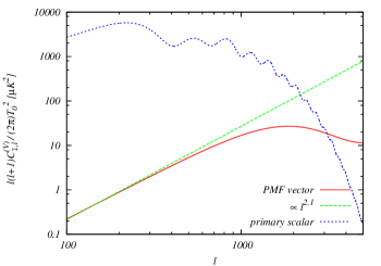
Figure 4: (color online). The CMB power spectra of temperature fluctuation. The lines correspond to the spectra generated from vector anisotropic stress of PMFs as Eq. (230) (red solid line) and primordial curvature perturbations (blue dotted line). The green dashed line express the asymptotic power of the red solid one. The PMF parameters are fixed to $n_{B}=-2.9$ and $B_{1{\rm Mpc}}=4.7{\rm nG}$, and the other cosmological parameters are fixed to the mean values limited from WMAP-7yr data reported in Ref. Komatsu et al. (2010).

References

- Bernet et al. (2008) M. L. Bernet, F. Miniati, S. J. Lilly, P. P. Kronberg, and M. Dessauges-Zavadsky, Nature 454, 302 (2008), eprint 0807.3347.
- Wolfe et al. (2008) A. M. Wolfe, R. A. Jorgenson, T. Robishaw, C. Heiles, and J. X. Prochaska, Nature 455, 638 (2008), eprint 0811.2408.
- Kronberg et al. (2008) P. P. Kronberg et al., Astrophys. J. 676, 70 (2008), eprint 0712.0435.
- Widrow (2002) L. M. Widrow, Rev. Mod. Phys. 74, 775 (2002), eprint astro-ph/0207240.
- Martin and Yokoyama (2008) J. Martin and J. Yokoyama, JCAP 0801, 025 (2008), eprint 0711.4307.
- Bamba and Sasaki (2007) K. Bamba and M. Sasaki, JCAP 0702, 030 (2007), eprint astro-ph/0611701.
- Stevens and Johnson (2010) T. Stevens and M. B. Johnson (2010), eprint 1001.3694.
- Kahniashvili et al. (2009) T. Kahniashvili, A. G. Tevzadze, and B. Ratra (2009), eprint 0907.0197.
- Ichiki et al. (2006) K. Ichiki, K. Takahashi, H. Ohno, H. Hanayama, and N. Sugiyama, Science. 311, 827 (2006), eprint astro-ph/0603631.
- Maeda et al. (2009) S. Maeda, S. Kitagawa, T. Kobayashi, and T. Shiromizu, Class. Quant. Grav. 26, 135014 (2009), eprint 0805.0169.
- Fenu et al. (2010) E. Fenu, C. Pitrou, and R. Maartens (2010), eprint 1012.2958.
- Lewis (2004a) A. Lewis, Phys. Rev. D70, 043011 (2004a), eprint astro-ph/0406096.
- Mack et al. (2002) A. Mack, T. Kahniashvili, and A. Kosowsky, Phys. Rev. D65, 123004 (2002), eprint astro-ph/0105504.
- Shaw and Lewis (2010) J. R. Shaw and A. Lewis, Phys. Rev. D81, 043517 (2010), eprint 0911.2714.
- Paoletti et al. (2009) D. Paoletti, F. Finelli, and F. Paci, Mon. Not. Roy. Astron. Soc. 396, 523 (2009), eprint 0811.0230.
- Subramanian and Barrow (1998a) K. Subramanian and J. D. Barrow, Phys. Rev. Lett. 81, 3575 (1998a), eprint astro-ph/9803261.
- Durrer et al. (1998) R. Durrer, T. Kahniashvili, and A. Yates, Phys. Rev. D58, 123004 (1998), eprint astro-ph/9807089.
- Brown and Crittenden (2005) I. Brown and R. Crittenden, Phys. Rev. D72, 063002 (2005), eprint astro-ph/0506570.
- Seshadri and Subramanian (2009) T. R. Seshadri and K. Subramanian, Phys. Rev. Lett. 103, 081303 (2009), eprint 0902.4066.
- Caprini et al. (2009) C. Caprini, F. Finelli, D. Paoletti, and A. Riotto, JCAP 0906, 021 (2009), eprint 0903.1420.
- Cai et al. (2010) R.-G. Cai, B. Hu, and H.-B. Zhang, JCAP 1008, 025 (2010), eprint 1006.2985.
- Trivedi et al. (2010) P. Trivedi, K. Subramanian, and T. R. Seshadri (2010), eprint 1009.2724.
- [Planck Collaboration] (2006) [Planck Collaboration] (2006), eprint astro-ph/0604069.
- Shiraishi et al. (2010a) M. Shiraishi, D. Nitta, S. Yokoyama, K. Ichiki, and K. Takahashi, Phys. Rev. D82, 121302 (2010a), eprint 1009.3632.
- Komatsu and Spergel (2001) E. Komatsu and D. N. Spergel, Phys. Rev. D63, 063002 (2001), eprint astro-ph/0005036.
- Kahniashvili and Lavrelashvili (2010) T. Kahniashvili and G. Lavrelashvili (2010), eprint 1010.4543.
- Kahniashvili (2011) T. Kahniashvili, private communication (2011).
- Shiraishi et al. (2011) M. Shiraishi, D. Nitta, S. Yokoyama, K. Ichiki, and K. Takahashi, Prog. Theor. Phys. 125, 795 (2011), eprint 1012.1079.
- Jedamzik et al. (1998) K. Jedamzik, V. Katalinic, and A. V. Olinto, Phys. Rev. D57, 3264 (1998), eprint astro-ph/9606080.
- Subramanian and Barrow (1998b) K. Subramanian and J. D. Barrow, Phys. Rev. D58, 083502 (1998b), eprint astro-ph/9712083.
- Hu and White (1997) W. Hu and M. J. White, Phys. Rev. D56, 596 (1997), eprint astro-ph/9702170.
- Zaldarriaga and Seljak (1997) M. Zaldarriaga and U. Seljak, Phys. Rev. D55, 1830 (1997), eprint astro-ph/9609170.
- Shiraishi et al. (2010b) M. Shiraishi, S. Yokoyama, D. Nitta, K. Ichiki, and K. Takahashi, Phys. Rev. D 82, 103505 (2010b).
- Hu (2001) W. Hu, Phys. Rev. D64, 083005 (2001), eprint astro-ph/0105117.
- Jahn and Hope (1954) H. A. Jahn and J. Hope, Phys. Rev. 93, 318 (1954).
- Gurau (2008) R. Gurau, Annales Henri Poincare 9, 1413 (2008), ISSN 1424-0637, eprint 0808.3533.
- (37) The wolfram function site, http://functions.wolfram.com/.
- Lewis et al. (2000) A. Lewis, A. Challinor, and A. Lasenby, Astrophys. J. 538, 473 (2000), eprint astro-ph/9911177.
- Lewis (2004b) A. Lewis, Phys. Rev. D 70, 043518 (2004b).
- (40) Slatec common mathematical library, http://www.netlib.org/slatec/.
- Komatsu et al. (2010) E. Komatsu et al. (2010), eprint 1001.4538.
- Riotto (2008) A. Riotto, in Inflationary Cosmology, edited by M. Lemoine, J. Martin, & P. Peter (2008), vol. 738 of Lecture Notes in Physics, Berlin Springer Verlag, pp. 305–+.
- Yamazaki et al. (2006) D. Yamazaki, K. Ichiki, T. Kajino, and G. J. Mathews, Astrophys. J. 646, 719 (2006), eprint astro-ph/0602224.