RI^′/SMOM scheme amplitudes for quark currents at two loops

Abstract. We determine the two loop corrections to the Green’s function of a quark current inserted in a quark $2$-point function at the symmetric subtraction point. The amplitudes for the scalar, vector and tensor currents are presented in both the $\overline{\mbox{MS}}$ and RI^′/SMOM renormalization schemes. The RI^′/SMOM scheme two loop renormalization for the scalar and tensor cases agree with previous work. The vector current renormalization requires special treatment as it must be consistent with the Slavnov-Taylor identity which we demonstrate. We also discuss the possibility of an alternative definition of the RI^′/SMOM scheme in the case of the tensor current.

LTH 906

1 Introduction.

Non-abelian quantum field theory underlies the strong nuclear force which binds quarks and gluons into hadrons. At high energy these quarks and gluons are asymptotically free, [1, 2], and so a good approximation to the physics of hadrons in deep inelastic scattering can be achieved by perturbation theory. When the coupling constant, $g$, is small then the only difficulty is the actual computation of a large number of Feynman diagrams which prevents one from obtaining precise estimates. However, the physics of the specific structure of hadrons resides in the non-perturbative or low energy régime where, because the coupling constant is large, then perturbation theory is not applicable. Instead one focuses on the computation of matrix elements involving the relevant operators for the hadrons or deep inelastic scattering process. In principle such matrix elements can be measured accurately by using a lattice regularization of the non-abelian gauge theory. If one has access to powerful enough computers then one can build a solid picture of the dependence of the matrix elements with momentum scales. One issue which arises in the lattice computations is that whilst concentrating on the low energy aspect, the resulting matrix elements must still match onto the high energy behaviour which one can calculate in perturbation theory. This is not a trivial exercise. For instance, the operators one has to consider undergo renormalization. In perturbation theory the anomalous dimensions of key operators are known to at least three loops. See, for instance, [3, 4, 5, 6, 7, 8, 9]. However, this is invariably in the standard (non-physical) renormalization scheme known as $\overline{\mbox{MS}}$. In this scheme essentially only the basic infinities with respect to the regularizing parameter are subtracted leaving the finite parts unsubtracted in the remaining part of the Green’s function. Invariably one uses dimensional regularization in $d$ $=$ $4$ $-$ $2\epsilon$ dimensions. Therefore, the finite parts of the matrix elements at high energy are a reflection of the scheme.

By contrast, the lattice uses various renormalization schemes which are different and physical. So to perform any matching in the overlap region requires knowledge of the matrix element in the same scheme whether this is $\overline{\mbox{MS}}$ or a lattice based scheme. The latter set of schemes are chosen primarily to reduce the financial cost of any numerical evaluation. For instance, derivatives within an operator or at any point require more computation. So the suite of lattice schemes are designed to minimize such complications. In earlier work the regularization invariant (RI) scheme and its modified version (RI^′) were defined in lattice computations, [10, 11], and later developed to three and four loops for the continuum in several articles, both for the Landau gauge, [12], and general linear covariant gauges, [13]. Indeed matrix elements for deep inelastic scattering operators were evaluated to three loops in RI^′ in [13, 14, 15]. More recently a variation on the RI^′ scheme has been developed, [16]. This is specifically related to matrix elements and designed to overcome a problem with potential infrared singularities. In essence the RI^′ scheme for $3$-point and higher Green’s functions involves subtracting the divergences at an exceptional momentum configuration. In other words the operator insertion is at zero momentum. To avoid this exceptional point and hence the related infrared issue, the RI^′/SMOM renormalization scheme was introduced, [16]. The annotation indicates that there is non nullification of any of the external momenta in a $3$-point function. Indeed the external momenta are non-zero and their squares are all fixed to be at the same value when the Green’s function is renormalized. Hence one refers to it as a symmetric subtraction point.

Initially this scheme was applied to the scalar, vector and tensor currents at one loop, [16], and to the scalar and tensor at two loops in [17, 18]. More recently it has been extended to various low moment operators used in deep inelastic scattering at one loop, [19]. However, the main focus of [17, 18] was the construction of the anomalous dimensions and thence the conversion functions from the RI^′/SMOM scheme to the $\overline{\mbox{MS}}$ one. These are central to any mapping of lattice results to the perturbative region for measurement comparisons. However, when one undertakes any measurement on the lattice the Green’s function with the operator insertion has free Lorentz indices and therefore it has to be written in terms of a set of basis tensors. Then different combinations of the free Lorentz indices can be determined and information on the associated scalar amplitudes extracted. Whilst [17, 18] concentrated on the operator renormalization, the explicit values of the individual two loop scalar amplitudes were not given which would be invaluable for lattice measurements. Therefore, it is the main purpose of this article to provide that information at two loops not only for the Green’s function with scalar and tensor current insertions to augment the work of [17, 18] but also for the vector current. This is partly because the latter has not been treated within the RI^′/SMOM formalism at two loops but mainly because it underlies the renormalization of the deep inelastic scattering operators considered at one loop in [19]. The amplitudes for those two sets of operators will be considered separately, [20]. The case of the vector current is special as its renormalization is connected with the Slavnov-Taylor identity as discussed in [16]. However, one feature of the tensor current is that the actual definition of the RI^′/SMOM scheme for such operators is not unique. This is because there is a relatively large set of basis tensors due to the free Lorentz indices. Therefore, a different basis choice would lead to different scheme definitions as we will indicate. In addition the way one projects out the part of the Green’s function whose finite part will be absorbed into the operator renormalization constant is also subject to a large degree of choice. As there is a range of ways of defining the RI^′/SMOM scheme for the tensor current we will give one alternative for illustration but will also present all the amplitudes for the currents considered here in the $\overline{\mbox{MS}}$ scheme too. So an interested reader has the liberty to toy with variations on the RI^′/SMOM scheme definition of [16, 17, 18].

The article is organized as follows. General aspects of the computations we perform as well as the techniques used to carry them out are given in section two. The three specific operators we consider and the details associated with each are discussed in the three subsequent sections. Aspects of the conversion functions are given in section six including that for the alternative scheme devised for the tensor current to allow one to contrast with that of [17, 18]. Our conclusions are given in section seven. The main results are presented in a series of Tables.

2 Preliminaries.

To start with we focus on the generalities of the computation we are interested in. The three basic quark currents are the scalar, vector and tensor currents and we use the compact notation introduced in [19, 21]

$$S~{}\equiv~{}\bar{\psi}\psi~{}~{}~{},~{}~{}~{}V~{}\equiv~{}\bar{\psi}\gamma^{\mu}\psi~{}~{}~{},~{}~{}~{}T~{}\equiv~{}\bar{\psi}\sigma^{\mu\nu}\psi$$ (2.1)

where $\sigma^{\mu\nu}$ $=$ $\mbox{\small{$\frac{1}{2}$}}[\gamma^{\mu},\gamma^{\nu}]$ is antisymmetric. Each of these operators, ${\cal O}$, is inserted into a quark $2$-point Green’s function where the two independent external momenta, $p$ and $q$, flow in through each external quark leg as illustrated in Figure $1$. As we will be concentrating on the renormalization of the operators and the consequent finite parts of the Green’s function of Figure $1$ at a symmetric renormalization point, we note that from here on we take, [16, 17, 18],

$$p^{2}~{}=~{}q^{2}~{}=~{}(p+q)^{2}~{}=~{}-~{}\mu^{2}$$ (2.2)

which implies

$$pq~{}=~{}\frac{1}{2}\mu^{2}$$ (2.3)

where $\mu$ is the mass scale associated with the renormalization point. At this point the Green’s function can be written in terms of a set of scalar amplitudes with respect to some basis of Lorentz tensors. Even though the scalar current has no free Lorentz indices there are two independent amplitudes as the two independent momenta lead to two independent structures deriving from the $\gamma$-matrices. This was discussed in [19] but we note that when either of the external momenta is nullified, equating to the RI^′ momentum configuration, then there is only one independent tensor in the basis. Therefore, in general we can write the Green’s function for each of our operators ${\cal O}^{i}_{\mu_{1}\ldots\mu_{n}}$ separately as

$$\left.\left\langle\psi(p){\cal O}^{i}_{\mu_{1}\ldots\mu_{n_{i}}}(-p-q)\bar{\psi}(q)\right\rangle\right|_{p^{2}=q^{2}=-\mu^{2}}~{}=~{}\sum_{k=1}^{n_{i}}{\cal P}^{i}_{(k)\,\mu_{1}\ldots\mu_{n_{i}}}(p,q)\,\Sigma^{{\cal O}^{i}}_{(k)}(p,q)$$ (2.4)

where $i$ is the label corresponding to the operator, which is either $S$, $V$ or $T$ here. The scalar amplitudes are denoted by $\Sigma^{{\cal O}^{i}}_{(k)}(p,q)$ with ${\cal P}^{i}_{(k)\,\mu_{1}\ldots\mu_{n_{i}}}(p,q)$ corresponding to the basis tensors. The latter were given in [19] and were derived by writing all the one loop Feynman diagrams in terms of a basic set of master tensor integrals. In other words each diagram was stripped of all features to leave purely basic integrals. These were evaluated by standard methods and then substituted back so that the computation could be completed by contracting the Lorentz indices with the stripped off $\gamma$-matrices. The reason for proceeding in this way was to ensure that no tensors contributing to the basis in the decompostion were omitted. Ordinarily one would construct the basis by building all possible tensors from the basic tensors such as $\eta_{\mu\nu}$, $\gamma$-matrices and independent momenta. Although here there are two momenta it turns out that even for simple currents the basis can be quite large. This is aside from the fact that we are only constructing the basis at the symmetric subtraction point where the values of $p^{2}$, $q^{2}$ and $(p+q)^{2}$ are all equal. Away from this point the basis of tensors will be significantly larger but we are not interested in the form of the amplitudes not at the symmetric point.

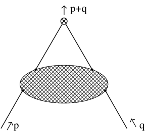
Figure 1: Momentum flow for the Green’s function, $\left\langle\psi(p){\cal O}^{i}_{\mu_{1}\ldots\mu_{n_{i}}}(-p-q)\bar{\psi}(q)\right\rangle$.

As the scalar amplitudes are the quantities we seek then it is possible to compute each individually via a projection onto the Green’s function itself. In other words

$$\Sigma^{{\cal O}^{i}}_{(k)}(p,q)~{}=~{}{\cal M}^{i}_{kl}{\cal P}^{i~{}\,\mu_{1}\ldots\mu_{n_{i}}}_{(l)}(p,q)\left.\left(\left\langle\psi(p){\cal O}^{i}_{\mu_{1}\ldots\mu_{n_{i}}}(-p-q)\bar{\psi}(q)\right\rangle\right)\right|_{p^{2}=q^{2}=-\mu^{2}}$$ (2.5)

where ${\cal M}^{i}_{kl}$ is a matrix of rational polynomials in $d$ with $k$ and $l$ labelling the different amplitudes relative to the ordering of the tensors in the basis, [19]. Thoughout we use dimensional regularization in $d$ $=$ $4$ $-$ $2\epsilon$ dimensions. This matrix is computed from the actual tensors themselves. First, if we define the matrix

$${\cal N}^{i}_{kl}~{}=~{}\left.{\cal P}^{i}_{(k)\,\mu_{1}\ldots\mu_{n_{i}}}(p,q){\cal P}^{i~{}\,\mu_{1}\ldots\mu_{n_{i}}}_{(l)}(p,q)\right|_{p^{2}=q^{2}=-\mu^{2}}$$ (2.6)

then ${\cal M}^{i}_{kl}$ is its inverse. Of course the choice of basis tensors is not unique and we use the one constructed for each operator at one loop. Whilst that involved stripping the spinor structure off all the Feynman graphs and then substituting the master tensor integrals, such an exercise would be too difficult and cumbersome to implement at two loops. Therefore, we use the projection of the Green’s function as outlined here. This was also used at one loop and reproduced the direct evaluation results of [19]. Therefore, we are confident that we have a complete basis. Though there are additional checks on the results such as agreement with the Slavnov-Taylor identity, in the case of the vector, as will be discussed later.

With our general decomposition of the Green’s function we can now discuss the renormalization and the method to define the RI^′/SMOM scheme renormalization constants. Of the set of scalar amplitudes, one or more will contain the poles in $\epsilon$. If we denote this amplitude, or set of amplitudes, by the label $0$ then the renormalization constant for the operator is defined by the condition, [16, 17, 18],

$$\left.\lim_{\epsilon\rightarrow 0}\left[Z^{\mbox{\footnotesize{RI${}^{\prime}$}}}_{\psi}Z^{\mbox{\footnotesize{RI${}^{\prime}$/SMOM}}}_{\cal O}\Sigma^{\cal O}_{(0)}(p,q)\right]\right|_{p^{2}\,=\,q^{2}\,=\,-\mu^{2}}~{}=~{}1~{}.$$ (2.7)

In other words there are no $O(a)$ corrections after renormalization where we set $a$ $=$ $g^{2}/(16\pi^{2})$ and $g$ is the coupling constant. In addition we note that the origin of the second aspect of this scheme definition is that the quark wave function renormalization is carried out in the RI^′ scheme. Briefly, this scheme is defined by ensuring that after renormalization there are no $O(a)$ corrections in $2$-point functions but for $3$-point functions and higher the renormalization is performed as one does in the $\overline{\mbox{MS}}$ scheme. This RI^′ scheme and its sister scheme, RI, were introduced in [10, 11] and examined in the continuum case at three and four loops, [12, 13, 14]. The latter work was for a linear covariant gauge fixing. Such computations are important when one is converting from schemes such as RI^′ or RI^′/SMOM to $\overline{\mbox{MS}}$ as one has to express the parameters of each scheme in terms of the same parameters of the other scheme. It transpires that the coupling constants are in direct correspondence, [13],

$$a_{\mbox{\footnotesize{RI${}^{\prime}$}}}~{}=~{}a_{\mbox{\footnotesize{$\overline{\mbox{MS}}$}}}~{}+~{}O\left(a_{\mbox{\footnotesize{$\overline{\mbox{MS}}$}}}^{5}\right)$$ (2.8)

to the order they were computed where we indicate the scheme to which the variables relate via the subscript. However, for a linear covariant gauge the gauge parameter, $\alpha$, is not in one-to-one correspondence except in the Landau gauge as, [13],

$$\alpha_{\mbox{\footnotesize{RI${}^{\prime}$}}} = \left[1+\left(\left(-9\alpha_{\mbox{\footnotesize{$\overline{\mbox{MS}}$}}}^{2}-18\alpha_{\mbox{\footnotesize{$\overline{\mbox{MS}}$}}}-97\right)C_{A}+80T_{F}N_{\!f}\right)\frac{a_{\mbox{\footnotesize{$\overline{\mbox{MS}}$}}}}{36}\right.$$ (2.9)

$$\left.~{}+~{}\left(\left(18\alpha_{\mbox{\footnotesize{$\overline{\mbox{MS}}$}}}^{4}-18\alpha_{\mbox{\footnotesize{$\overline{\mbox{MS}}$}}}^{3}+190\alpha_{\mbox{\footnotesize{$\overline{\mbox{MS}}$}}}^{2}-576\zeta(3)\alpha_{\mbox{\footnotesize{$\overline{\mbox{MS}}$}}}+463\alpha_{\mbox{\footnotesize{$\overline{\mbox{MS}}$}}}+864\zeta(3)-7143\right)C_{A}^{2}\right.\right.$$

$$\left.\left.~{}~{}~{}~{}~{}~{}~{}+~{}\left(-~{}320\alpha_{\mbox{\footnotesize{$\overline{\mbox{MS}}$}}}^{2}-320\alpha_{\mbox{\footnotesize{$\overline{\mbox{MS}}$}}}+2304\zeta(3)+4248\right)C_{A}T_{F}N_{\!f}\right.\right.$$

$$\left.\left.~{}~{}~{}~{}~{}~{}~{}+~{}\left(-~{}4608\zeta(3)+5280\right)C_{F}T_{F}N_{\!f}\right)\frac{a^{2}_{\mbox{\footnotesize{$\overline{\mbox{MS}}$}}}}{288}\right]\alpha_{\mbox{\footnotesize{$\overline{\mbox{MS}}$}}}~{}+~{}O\left(a^{3}_{\mbox{\footnotesize{$\overline{\mbox{MS}}$}}}\right)$$

to two loops. The full three loop result is given in [13]. These relations between the parameters of each scheme are required when converting the amplitudes. The group Casimirs are defined in the usual way by

$$T^{a}T^{a}~{}=~{}C_{F}~{}~{}~{},~{}~{}~{}f^{acd}f^{bcd}~{}=~{}C_{A}\delta^{ab}~{}~{}~{},~{}~{}~{}\mbox{Tr}\left(T^{a}T^{b}\right)~{}=~{}T_{F}\delta^{ab}$$ (2.10)

where $T^{a}$ are the generators of the colour group whose structure functions are $f^{abc}$. Throughout we work with $N_{\!f}$ massless quarks so that all our expressions for amplitudes are for the chiral limit. In principle quark masses could be included. However, the basic master scalar Feynman integrals at two loops with massive propagators are not known exactly for the symmetric point. So quark mass dependence for the scalar amplitudes of the Green’s function we are computing could only be determined in, say, the small quark mass limit. In connection with the relation of the parameters between schemes we should note that in [16] a different parameter mapping was chosen. There it was assumed that the gauge parameter was the same in both schemes in the same way that the coupling constants are. Here we will present all our results for the non-Landau schemes in what we regard as the full RI^′ context which led to (2.9).

The next aspect of (2.7) which we need to draw attention to is the way in which the operator renormalization constant is actually defined. For instance, in writing (2.7) we are making a basis dependent statement. The choice of the basis tensors is purely arbitrary and another choice with the same underlying criterion of having no $O(a)$ correction will clearly lead to a different numerical value of the corrections in the renormalization constant itself. Moreover, the amplitudes will also have the same degree of arbitrariness. This is not the same as scheme dependence. In that situation if one could compute the amplitudes to all orders the physics would not be affected by the renormalization scheme choice. However, as one has to truncate series in quantum field theory due to the limit of calculability it is clear that the construction of conversion functions, such as those of [16, 17, 18], could be affected by the basis choice. Though in [16, 17, 18] the approach used was to project the Green’s function with the appropriate Born term before rendering that projection to have no $O(a)$ part. This defined the RI^′/SMOM scheme for the scalar and tensor currents. However, once the full scalar amplitudes have been computed it is clear that there is in fact a sizeable number of ways of defining a so called RI^′/SMOM scheme. This was discussed in the one loop context in [19] where it is becomes a more important issue for the operators used in deep inelastic scattering. Therefore, we will discuss a possible variation on the scheme of [17, 18] for the tensor current at two loops. In addition, partly because of these general aspects we will provide all the amplitudes in the reference $\overline{\mbox{MS}}$ scheme. This is primarily for lattice computations where it is easier to convert to $\overline{\mbox{MS}}$ on the lattice before looking at the matching onto the ultraviolet part of the Green’s function where perturbation theory is valid.

Next we address some of the technical aspects of the computation. One feature of the basis of tensors is that they involve products of $\gamma$-matrices. This is because one can have contractions such as $p\!\!\!/$ and $q\!\!\!/$. Therefore, we have chosen to work with the generalized $\Gamma$-matrices of [22, 23, 24] which are denoted by $\Gamma_{(n)}^{\mu_{1}\ldots\mu_{n}}$. They are defined by

$$\Gamma_{(n)}^{\mu_{1}\ldots\mu_{n}}~{}=~{}\gamma^{[\mu_{1}}\ldots\gamma^{\mu_{n}]}$$ (2.11)

which is totally antisymmetric in all the Lorentz indices and the notation includes the overall factor of $1/n!$. So, for instance, $\sigma^{\mu\nu}$ $=$ $\Gamma_{(2)}^{\mu\nu}$. General properties are given in [25, 26]. One advantage of this choice for the tensor basis is that in $\Gamma$-space

$$\mbox{tr}\left(\Gamma_{(m)}^{\mu_{1}\ldots\mu_{m}}\Gamma_{(n)}^{\nu_{1}\ldots\nu_{n}}\right)~{}\propto~{}\delta_{mn}I^{\mu_{1}\ldots\mu_{m}\nu_{1}\ldots\nu_{n}}$$ (2.12)

where $I^{\mu_{1}\ldots\mu_{m}\nu_{1}\ldots\nu_{n}}$ is the unit matrix in this space. So there is a natural partition for the basis. The main tool to handle the tedious algebra for manipulating tensor projections is the symbolic manipulation language Form, [27]. The Feynman diagrams are generated with the Qgraf package, [28], and converted into Form notation whereby the colour and Lorentz indices are appended. For the Green’s function we are interested in with quark current insertions there are $1$ one loop graph and $13$ two loop graphs to be computed. These graphs are readily broken up into a set of tensor integrals where the external momenta swamp any free Lorentz index when we have multiplied by the appropriate tensor of the projection basis. As these integrals are in essence $3$-point functions evaluated at the symmetric point the next stage is to break them down into the known scalar master integrals. These are collected in [16] but were derived in various articles, [29, 30, 31, 32]. The engine room of this aspect of the computation is the Laporta algorithm, [33]. Briefly, that method allows one to build a redundant set of equations where basic Feynman graphs with irreducible numerators are all related by integration by parts and Lorentz identities. These can then be solved as a tower of equations with the master integrals being the foundation for the many sets of integrals in predefined sectors. There are a variety of computer packages available to build a Laporta system, [34, 35]. However, we have used Reduze, [36], which uses Ginac, [37], and involves C$++$ at its root. For the particular Green’s function we consider we need only build two topologies using the Reduze package since all the Feynman graphs are either based on a two loop ladder or the non-planar ladder. Once the system is built it can be converted into Form language and all the two loop tensor integrals for all the Feynman graphs at the symmetric subtraction point are written in terms of the known scalar master integrals listed in [18]. A check on the Reduze results is that we do reproduce the expressions given in [16, 17, 18]. Though the expressions we give at two loops for the amplitudes are new.

As was evident in [17, 18] the final forms for the two loop anomalous dimensions and associated conversion functions were surprisingly long. As we will be presenting a large number of amplitudes for the three currents in two renormalization schemes in order to save space we will collect the main results in Tables. To do this we have had to split the amplitudes by their colour group structure and so we have defined

$$\Sigma^{{\cal O}^{i}}_{(i)}(p,q) = \left(\sum_{n}c^{{\cal O}^{i},(1)}_{(i)\,n}a^{(1)}_{n}\right)C_{F}a~{}+~{}\left(\sum_{n}c^{{\cal O}^{i},(21)}_{(i)\,n}a^{(21)}_{n}\right)C_{F}T_{F}N_{\!f}a^{2}$$ (2.13)

$$+~{}\left(\sum_{n}c^{{\cal O}^{i},(22)}_{(i)\,n}a^{(22)}_{n}\right)C_{F}C_{A}a^{2}~{}+~{}\left(\sum_{n}c^{{\cal O}^{i},(23)}_{(i)\,n}a^{(23)}_{n}\right)C_{F}^{2}a^{2}~{}+~{}O(a^{3})$$

where the parameters are in either scheme. Here we will adapt the convention that all expressions are in the RI^′/SMOM scheme unless explicitly indicated to be in the $\overline{\mbox{MS}}$ scheme. The coupling constants are the same but the gauge parameters are not, (2.9). In (2.13) the entities $a_{n}^{(k)}$ denote the basis of numbers which appear in that specific part of anomalous dimension. This includes, for instance, the gauge parameter dependence and it is evident from the left hand column of each table what these numbers actually are for each colour structure. In essence they relate to the form of the scalar master integrals at the symmetric subtraction point. The other entities, $c^{{\cal O}^{i},(k)}_{(i)\,n}$, are the actual coefficients of the number basis. The summation label $n$ corresponds to the row of each table. The superscript $k$ annotates the loop order, as the first number, and at two loop the second number references the colour group structure. Although the exact expressions at two loop represent all the information on the scalar amplitudes which we seek, we have relegated the Tables to the end of the article as it is the numerical evaluation which is ultimately of practical use. These expressions will be provided for each operator in succession in the next few sections. Throughout the one loop amplitudes are in agreement with those of [16].

3 Scalar current.

In this section we concentrate on the scalar current. The aim for this and the other currents is to provide not only the anomalous dimensions in the full RI^′/SMOM scheme but also the finite parts of all the amplitudes. Previously in [17, 18] the two loop anomalous dimension and conversion function were given. However, in order to assist with the extraction of results from the lattice, measurements have to be made in different components of the Lorentz basis of tensors and therefore all the finite parts of the Green’s functions need to be known accurately. As the amplitudes for the scalar current have not been given at two loops we briefly report on this situation in this section first. The decomposition into the projection tensors involves two tensors which are

$${\cal P}^{S}_{(1)}(p,q)~{}=~{}\Gamma_{(0)}~{}~{}~{},~{}~{}~{}{\cal P}^{S}_{(2)}(p,q)~{}=~{}\frac{1}{\mu^{2}}\Gamma_{(2)}^{pq}$$ (3.1)

where we use the convention that if a momentum is contracted with a Lorentz index of $\Gamma_{(n)}^{\mu_{1}\ldots\mu_{n}}$ then we replace that index by the momentum to save space. The matrix used for constructing the explicit projection is given by, [19],

$${\cal M}^{S}~{}=~{}\frac{1}{12}\left(\begin{array}[]{cc}3&0\\ 0&-4\\ \end{array}\right)~{}.$$ (3.2)

This is a simple example of the partitioning of the matrix as a consequence of the choice of the $\Gamma_{(n)}$ basis. As noted previously to record the full two loop expressions for the amplitudes would be demanding on space. However, as there are only two amplitudes for the scalar case we present the results for both schemes in Tables $1$ to $4$. The notation of (2.13) is used with the convention that the $\overline{\mbox{MS}}$ scheme results are annotated explicitly. Otherwise the results are in the RI^′/SMOM scheme. For the scalar current the RI^′/SMOM scheme renormalization condition is to project the Green’s function with the Born term and then define the operator renormalization constant so that there is no $O(a)$ finite part, [16, 17, 18]. Since we are using the generalized $\Gamma$-matrix basis then for the scalar case this equates to ensuring that there are no $O(a)$ corrections to the channel $1$ amplitude. This is because of (2.12). Consequently there are no RI^′/SMOM scheme coefficients for channel $1$ in these Tables.

Throughout we use the standard basis for the numbers which appear in this symmetric subtraction point momentum configuration for this Green’s function, [17]. There $\psi(z)$ is the derivative of the logarithm of the Euler Gamma function,

$$s_{n}(z)~{}=~{}\frac{1}{\sqrt{3}}\Im\left[\mbox{Li}_{n}\left(\frac{e^{iz}}{\sqrt{3}}\right)\right]$$ (3.3)

where $\mbox{Li}_{n}(z)$ is the polylogarithm function, $\zeta(z)$ is the Riemann zeta function and $\Sigma$ is given by a combination of various harmonic polylogarithms, [17, 32],

$$\Sigma~{}=~{}{\cal H}^{(2)}_{31}~{}+~{}{\cal H}^{(2)}_{43}~{}.$$ (3.4)

Whilst the exact two loop expressions are the output from the Form computation, for practical purposes expressing the result in numerical form will be more pragmatic for users. Therefore, we record this in an explicit equation for the case of $SU(3)$ not only for the scalar operator but also for the other cases we consider later. For the $\overline{\mbox{MS}}$ scheme we have

$$\left.\Sigma^{S}_{(1)}(p,q)\right|_{\overline{\mbox{\footnotesize{MS}}}} = -~{}1~{}-~{}\left[1.1040618\alpha+0.6455188\right]a$$

$$-~{}\left[48.4885881+7.58534654\alpha+3.67844381\alpha^{2}-6.3468728N_{\!f}\right]a^{2}~{}+~{}O(a^{3})$$

$$\left.\Sigma^{S}_{(2)}(p,q)\right|_{\overline{\mbox{\footnotesize{MS}}}} = \left[1.0417366\alpha-1.0417366\right]a$$ (3.5)

$$-~{}\left[11.1668053-7.37922016\alpha-3.5592665\alpha^{2}-0.4629940N_{\!f}\right]a^{2}$$

$$+~{}O(a^{3})~{}.$$

Those for the RI^′/SMOM scheme are

$$\Sigma^{S}_{(1)}(p,q) = -~{}1~{}+~{}O(a^{3})$$

$$\Sigma^{S}_{(2)}(p,q) = \left[1.0417366\alpha-1.0417366\right]a$$ (3.6)

$$-~{}\left[10.4943447-16.2776049\alpha-3.97172981\alpha^{2}-0.7813024\alpha^{3}\right.$$

$$\left.~{}~{}~{}~{}+~{}\left[1.1574851\alpha-0.4629940\right]N_{\!f}\right]a^{2}~{}+~{}O(a^{3})~{}.$$

Throughout we use the numerical values

$$\zeta(3) = 1.20205690~{}~{},~{}~{}\Sigma~{}=~{}6.34517334~{}~{},~{}~{}\psi^{\prime}\left(\frac{1}{3}\right)~{}=~{}10.09559713$$

$$\psi^{\prime\prime\prime}\left(\frac{1}{3}\right) = 488.1838167~{}~{},~{}~{}s_{2}\left(\frac{\pi}{2}\right)~{}=~{}0.32225882~{}~{},~{}~{}s_{2}\left(\frac{\pi}{6}\right)~{}=~{}0.22459602$$

$$s_{3}\left(\frac{\pi}{2}\right) = 0.32948320~{}~{},~{}~{}s_{3}\left(\frac{\pi}{6}\right)~{}=~{}0.19259341~{}.$$ (3.7)

Clearly there is a weak dependence on the number of quarks in channel $2$. To reinforce an earlier point the gauge parameter $\alpha$ in these sets of expressions is the variable in the RI^′/SMOM scheme. Though the coupling constant, $a$, is in the same scheme it is an exact map of the $\overline{\mbox{MS}}$ variable. Moreover, as with other RI^′/SMOM scheme anomalous dimensions of gauge invariant operators the higher loop corrections will depend on the gauge parameter. This is because the scheme is a mass dependent one and not a mass independent one like $\overline{\mbox{MS}}$. Finally, we note that using (2.9) the RI^′/SMOM scheme anomalous dimension is

$$\left.\frac{}{}\gamma^{S}(a,\alpha)\right|_{\mbox{\footnotesize{RI${}^{\prime}$/SMOM}}} = -~{}3C_{F}a$$ (3.8)

$$+~{}\left[\left[(3\alpha^{2}+9\alpha+66)\psi^{\prime}(\mbox{\small{$\frac{1}{3}$}})-(2\alpha^{2}+6\alpha+44)\pi^{2}\right.\right.$$

$$\left.\left.~{}~{}~{}~{}~{}-~{}9\alpha^{2}-27\alpha-555\right]C_{A}~{}-~{}27C_{F}\right.$$

$$\left.~{}~{}~{}~{}+~{}\left[16\pi^{2}+156-24\psi^{\prime}(\mbox{\small{$\frac{1}{3}$}})\right]T_{F}N_{\!f}\right]\frac{C_{F}a^{2}}{18}~{}+~{}O(a^{3})$$

which agrees with [16, 17, 18] when $\alpha$ $=$ $0$ where we will annotate the anomalous dimensions with the scheme. The $\alpha$ dependent terms differ because of the different ways the renormalization of $\alpha$ is performed. We have chosen to define the $\alpha$ renormalization using the RI^′ scheme of [13] whereas in [17] the $\alpha$ renormalization is taken to be in the $\overline{\mbox{MS}}$ scheme. As ultimately lattice computations are in the Landau gauge this difference in definitions would only be important in non-Landau linear covariant gauges.

4 Vector current.

As the vector operator has not received attention at two loops, we devote this section to it in detail using the general notation discussed previously. First, the basis of tensors used to decompose the Green’s function at the symmetric subtraction point is, [19],

$${\cal P}^{V}_{(1)\mu}(p,q) = \gamma_{\mu}~{}~{}~{},~{}~{}~{}{\cal P}^{V}_{(2)\mu}(p,q)~{}=~{}\frac{{p}^{\mu}p\!\!\!/}{\mu^{2}}~{}~{}~{},~{}~{}~{}{\cal P}^{V}_{(3)\mu}(p,q)~{}=~{}\frac{{p}_{\mu}q\!\!\!/}{\mu^{2}}~{},$$

$${\cal P}^{V}_{(4)\mu}(p,q) = \frac{{q}_{\mu}p\!\!\!/}{\mu^{2}}~{}~{}~{},~{}~{}~{}{\cal P}^{V}_{(5)\mu}(p,q)~{}=~{}\frac{{q}_{\mu}q\!\!\!/}{\mu^{2}}~{}~{}~{},~{}~{}~{}{\cal P}^{V}_{(6)\mu}(p,q)~{}=~{}\frac{1}{\mu^{2}}\Gamma_{(3)\,\mu pq}~{},$$ (4.1)

where the matrix used to perform the projection into the various amplitudes is, [19],

$${\cal M}^{V}~{}=~{}\frac{1}{36(d-2)}\left(\begin{array}[]{cccccc}9&12&6&6&12&0\\ 12&16(d-1)&8(d-1)&8(d-1)&4(d+2)&0\\ 6&8(d-1)&4(4d-7)&4(d-1)&8(d-1)&0\\ 6&8(d-1)&4(d-1)&4(4d-7)&8(d-1)&0\\ 12&4(d+2)&8(d-1)&8(d-1)&16(d-1)&0\\ 0&0&0&0&0&-12\\ \end{array}\right)~{}.$$ (4.2)

With this setup we have applied the computational algorithm to extract the RI^′/SMOM renormalization constant. To do this for the RI^′/SMOM scheme requires a different approach compared to the other quark currents. The reason for this is that the vector current is a physical operator and therefore its renormalization is already determined by general considerations. Specifically as it is physical its anomalous dimension is zero which is widely known in the $\overline{\mbox{MS}}$ scheme. However, once it is accepted that the renormalization constant is unity in one scheme then it is unity in all other schemes, [38]. Underlying this is the Slavnov-Taylor identity which relates the renormalization of the Green’s function with the divergence of the operator to the renormalization of the quark $2$-point functions. Indeed this was discussed in [13] for the RI^′ scheme and demonstrated to be consistent to three loops. The situation for the RI^′/SMOM computation is more involved as there are two momenta flowing through the Green’s function with the operator insertion. Therefore, to reproduce the Slavnov-Taylor identity the Green’s function of Figure $1$ has to be contracted with the vector $(p+q)_{\mu}$. This is one reason why we have to decompose the Green’s function into a basis of projection tensors. Once we have established this then the contraction can proceed. For the case of the RI^′ scheme this aspect of the reconciliation with the Slavnov-Taylor identity is simplified significantly because there is only one momentum flowing through the Green’s function. Indeed put another way the contraction of the graph of Figure $1$ with $(p+q)_{\mu}$ will effectively become the renormalization condition for $Z^{V}$ but will naturally produce unity as expected from general theorems. Whilst we are focusing on this feature for the vector current in detail here it transpires that the same issue arises for operators which are used in deep inelastic scattering. This was discussed at one loop in [19] for the sets of operators labelled $W_{2}$ and $W_{3}$ in the notation of [21]. This is because the contraction of Lorentz indices of one of the operators in each set is equivalent to the divergence of the vector current. Therefore, the renormalization of those operators also has to be consistent with the Slavnov-Taylor identity.

To focus on the issue we concentrate on the $\overline{\mbox{MS}}$ renormalization first. The explicit results for each of the amplitudes is given in Tables $5$ to $8$. The numerical values for the amplitudes for $SU(3)$ are

$$\left.\Sigma^{V}_{(1)}(p,q)\right|_{\overline{\mbox{\footnotesize{MS}}}} = -~{}1~{}+~{}\left[1.6249301-0.5831936\alpha\right]a$$

$$+~{}\left[6.1248321-3.2229010\alpha-1.8119992\alpha^{2}+0.2362586N_{\!f}\right]a^{2}~{}+~{}O(a^{3})$$

$$\left.\Sigma^{V}_{(2)}(p,q)\right|_{\overline{\mbox{\footnotesize{MS}}}} = \left.\Sigma^{V}_{(5)}(p,q)\right|_{\overline{\mbox{\footnotesize{MS}}}}$$

$$= \left[1.4720824+0.3056953\alpha\right]a$$

$$+~{}\left[18.7974908+4.5957818\alpha+1.0954082\alpha^{2}-1.3299518N_{\!f}\right]a^{2}~{}+~{}O(a^{3})$$

$$\left.\Sigma^{V}_{(3)}(p,q)\right|_{\overline{\mbox{\footnotesize{MS}}}} = \left.\Sigma^{V}_{(4)}(p,q)\right|_{\overline{\mbox{\footnotesize{MS}}}}$$

$$= \left[1.7777778+1.1945842\alpha\right]a$$

$$+~{}\left[44.3805855+12.1090504\alpha+4.2805934\alpha^{2}-2.8641975N_{\!f}\right]a^{2}~{}+~{}O(a^{3})$$

$$\left.\Sigma^{V}_{(6)}(p,q)\right|_{\overline{\mbox{\footnotesize{MS}}}} = -~{}2.0834731a$$ (4.3)

$$-~{}\left[39.7873696+0.3484662\alpha+0.1736228\alpha^{3}-3.0094611N_{\!f}\right]a^{2}$$

$$+~{}O(a^{3})~{}.$$

As noted at one loop in [19] there is a degree of symmetry which is also evident at two loops. This is primarily due to the way in which we chose our basis of Lorentz tensors which is of course not unique. The fact that various channels pair off to two loops can be regarded as an internal check on both the construction of the projection matrix and the symbolic manipulation code used to perform the computation. In the tables for the vector case we do not reproduce columns for the channels $4$ and $5$ because of the above equalities which hold exactly to two loops. In order to see that the Slavnov-Taylor identity is satisfied to two loops in the $\overline{\mbox{MS}}$ scheme we have computed that combination of the amplitudes which correspond to the Green’s function of the insertion of the divergence of the vector current. With the contraction with $(p+q)_{\mu}$ there will be two terms. One will involve $p\!\!\!/$ and the other $q\!\!\!/$. For the former the combination gives

$$\left.\Sigma^{V}_{(1)}(p,q)\right|_{\overline{\mbox{\footnotesize{MS}}}}~{}-~{}\frac{1}{2}\left.\Sigma^{V}_{(2)}(p,q)\right|_{\overline{\mbox{\footnotesize{MS}}}}~{}-~{}\frac{1}{2}\left.\Sigma^{V}_{(5)}(p,q)\right|_{\overline{\mbox{\footnotesize{MS}}}}$$

$$=~{}-~{}1~{}-~{}\alpha C_{F}a~{}+~{}\left[\left[3\zeta(3)-\frac{41}{4}+3\zeta(3)\alpha-\frac{13}{2}\alpha-\frac{9}{8}\alpha^{2}\right]C_{A}+\frac{5}{8}C_{F}+\frac{7}{2}T_{F}N_{\!f}\right]C_{F}a^{2}$$

$$~{}~{}~{}~{}+~{}O(a^{3})$$ (4.4)

and that for the latter is a different combination of amplitudes but produces the same result. The right hand side of (4.4) is clearly the finite part of the quark $2$-point function after renormalizing in the $\overline{\mbox{MS}}$ scheme. Therefore, given the fact that the Green’s function is symmetric under interchange of $p$ and $q$ then this shows that the Slavnov-Taylor identity is correctly embedded within our computation with the vector current having a renormalization constant of unity.

The situation for the RI^′/SMOM scheme amplitudes is completely parallel to that of $\overline{\mbox{MS}}$. We have given the amplitudes for this case in Tables $9$ to $12$ where we have used

$$Z^{V}~{}=~{}1~{}+~{}O(a^{3})$$ (4.5)

for the renormalization of the vector current. As a brief summary the $SU(3)$ numerical values are

$$\Sigma^{V}_{(1)}(p,q) = -~{}1~{}+~{}\left[1.6249301+0.7501398\alpha\right]a$$

$$+~{}\left[31.5890381+12.2494724\alpha+2.8130241\alpha^{2}+0.5626048\alpha^{3}\right.$$

$$\left.~{}~{}~{}~{}-~{}\left[2.0970747+0.8334886\alpha\right]N_{\!f}\right]a^{2}~{}+~{}O(a^{3})$$

$$\Sigma^{V}_{(2)}(p,q) = \Sigma^{V}_{(5)}(p,q)$$

$$= \left[1.4720824+0.3056953\alpha\right]a$$

$$+~{}\left[18.7974908+5.1040424\alpha+1.1463575\alpha^{2}+0.2292715\alpha^{3}\right.$$

$$\left.~{}~{}~{}~{}-~{}\left[1.3299518+0.3396615\alpha\right]N_{\!f}\right]a^{2}~{}+~{}O(a^{3})$$

$$\Sigma^{V}_{(3)}(p,q) = \Sigma^{V}_{(4)}(p,q)$$

$$= \left[1.7777778+1.1945842\alpha\right]a$$

$$+~{}\left[44.3805855+19.3949024\alpha+4.4796908\alpha^{2}+0.8959382\alpha^{3}\right.$$

$$\left.~{}~{}~{}~{}-~{}\left[2.8641975+1.3273158\alpha\right]N_{\!f}\right]a^{2}~{}+~{}O(a^{3})$$

$$\Sigma^{V}_{(6)}(p,q) = -~{}2.0834731a$$ (4.6)

$$-~{}\left[39.7873696-2.4294979\alpha+0.1736228\alpha^{2}-3.0094611N_{\!f}\right]a^{2}$$

$$+~{}O(a^{3})~{}.$$

In order to see that the definition of $Z^{V}$ is consistent with the Slavnov-Taylor identity we have repeated the computation of (4.4) for the RI^′/SMOM amplitudes. In this case the piece involving $p\!\!\!/$ produces

$$\Sigma^{V}_{(1)}(p,q)~{}-~{}\frac{1}{2}\Sigma^{V}_{(2)}(p,q)~{}-~{}\frac{1}{2}\Sigma^{V}_{(5)}(p,q)~{}=~{}-~{}1~{}+~{}O(a^{3})~{}.$$ (4.7)

Here there are no corrections which is consistent with the RI^′/SMOM scheme since, [16], it uses the RI^′ quark wave function renormalization. This is chosen in such a way that the quark $2$-point function has no $O(a)$ corrections. In other words the finite part of that $2$-point function is absorbed into the finite part of the wave function renormalization constant. Therefore, the vector current anomalous dimension

$$\left.\frac{}{}\gamma^{V}(a,\alpha)\right|_{\mbox{\footnotesize{RI${}^{\prime}$/SMOM}}}~{}=~{}O(a^{3})$$ (4.8)

is consistent with the underlying Slavnov-Taylor identity. Whilst $\left.\frac{}{}\gamma^{V}(a,\alpha)\right|_{\mbox{\footnotesize{RI${}^{\prime}$/SMOM}}}$ is zero to all orders we include the order symbol merely to record the order to which we have explicitly verified this to.

5 Tensor current.

Next we record the parallel situation for the tensor operator noting only the points where there are differences from earlier work and discussions. The Lorentz tensor basis for the amplitude decomposition is, [19],

$${\cal P}^{T}_{(1)\mu\nu}(p,q) = \Gamma_{(2)\,\mu\nu}~{}~{}~{},~{}~{}~{}{\cal P}^{T}_{(2)\mu\nu}(p,q)~{}=~{}\frac{1}{\mu^{2}}\left[p_{\mu}q_{\nu}-p_{\nu}q_{\mu}\right]\Gamma_{(0)}~{},$$

$${\cal P}^{T}_{(3)\mu\nu}(p,q) = \frac{1}{\mu^{2}}\left[\Gamma_{(2)\,\mu p}p_{\nu}-\Gamma_{(2)\,\nu p}p_{\mu}\right]~{}~{}~{},~{}~{}~{}{\cal P}^{T}_{(4)\mu\nu}(p,q)~{}=~{}\frac{1}{\mu^{2}}\left[\Gamma_{(2)\,\mu p}q_{\nu}-\Gamma_{(2)\,\nu p}q_{\mu}\right]~{},$$

$${\cal P}^{T}_{(5)\mu\nu}(p,q) = \frac{1}{\mu^{2}}\left[\Gamma_{(2)\,\mu q}p_{\nu}-\Gamma_{(2)\,\nu q}p_{\mu}\right]~{}~{}~{},~{}~{}~{}{\cal P}^{T}_{(6)\mu\nu}(p,q)~{}=~{}\frac{1}{\mu^{2}}\left[\Gamma_{(2)\,\mu q}q_{\nu}-\Gamma_{(2)\,\nu q}q_{\mu}\right]~{},$$

$${\cal P}^{T}_{(7)\mu\nu}(p,q) = \frac{1}{\mu^{4}}\left[\Gamma_{(2)\,pq}p_{\mu}q_{\nu}-\Gamma_{(2)\,pq}p_{\nu}q_{\mu}\right]~{}~{}~{},~{}~{}~{}{\cal P}^{T}_{(8)\mu\nu}(p,q)~{}=~{}\frac{1}{\mu^{2}}\Gamma_{(4)\,\mu\nu pq}~{}.$$ (5.1)

The matrix to determine the explicit projection is defined as, [19],

$${\cal M}^{T}~{}=~{}\frac{1}{36(d-2)(d-3)}\left(\begin{array}[]{cc}{\cal M}^{T}_{11}&{\cal M}^{T}_{12}\\ {\cal M}^{T}_{21}&{\cal M}^{T}_{22}\\ \end{array}\right)$$ (5.2)

with the four submatrices given by

$${\cal M}^{T}_{11} = \left(\begin{array}[]{cccc}-9&0&-12&-6\\ 0&6(d-2)(d-3)&0&0\\ -12&0&-8(d-1)&-4(d-1)\\ -6&0&-4(d-1)&-4(2d-5)\\ \end{array}\right)~{},$$ (5.7)

$${\cal M}^{T}_{12} = \left(\begin{array}[]{cccc}-6&-12&-12&-6\\ 0&0&0&0\\ -4(d-1)&-2(d+5)&-8(d-1)&0\\ -2(d-1)&-4(d-1)&-4(d-1)&0\\ \end{array}\right)~{},$$ (5.12)

$${\cal M}^{T}_{21} = \left(\begin{array}[]{cccc}-6&0&-4(d-1)&-2(d-1)\\ -12&0&-2(d+5)&-4(d-1)\\ -12&0&-8(d-1)&-4(d-1)\\ 0&0&0&0\\ \end{array}\right)~{},$$ (5.17)

$${\cal M}^{T}_{22} = \left(\begin{array}[]{cccc}-4(2d-5)&-4(d-1)&-4(d-1)&0\\ -4(d-1)&-8(d-1)&-8(d-1)&0\\ -4(d-1)&-8(d-1)&-8(d-1)(d-2)&0\\ 0&0&0&12\\ \end{array}\right)~{}.$$ (5.22)

This produces the two loop $\overline{\mbox{MS}}$ numerical values for the amplitudes

$$\left.\Sigma^{T}_{(1)}(p,q)\right|_{\overline{\mbox{\footnotesize{MS}}}} = -~{}1~{}+~{}\left[0.0623253-0.0623253\alpha\right]a$$

$$+~{}\left[17.0099539+0.6409422\alpha+0.0544455\alpha^{2}-1.6001145N_{\!f}\right]a^{2}~{}+~{}O(a^{3})$$

$$\left.\Sigma^{T}_{(2)}(p,q)\right|_{\overline{\mbox{\footnotesize{MS}}}} = \left[3.1252097+1.0417366\alpha\right]a$$

$$+~{}\left[76.2022091+10.8541168\alpha+3.9065121\alpha^{2}-5.5559283N_{\!f}\right]a^{2}$$

$$+~{}O(a^{3})$$

$$\left.\Sigma^{T}_{(3)}(p,q)\right|_{\overline{\mbox{\footnotesize{MS}}}} = \left.\Sigma^{T}_{(6)}(p,q)\right|_{\overline{\mbox{\footnotesize{MS}}}}$$

$$= \left[0.3056953\alpha-0.3056953\right]a$$

$$-~{}\left[1.8195802-3.2067998\alpha-1.0954082\alpha^{2}-0.3396615N_{\!f}\right]a^{2}~{}+~{}O(a^{3})$$

$$\left.\Sigma^{T}_{(4)}(p,q)\right|_{\overline{\mbox{\footnotesize{MS}}}} = \left.\Sigma^{T}_{(5)}(p,q)\right|_{\overline{\mbox{\footnotesize{MS}}}}$$

$$= \left[0.1528477\alpha-0.1528477\right]a$$

$$-~{}\left[0.9097901-1.6033999\alpha-0.5477041\alpha^{2}-0.1698307N_{\!f}\right]a^{2}~{}+~{}O(a^{3})$$

$$\left.\Sigma^{T}_{(7)}(p,q)\right|_{\overline{\mbox{\footnotesize{MS}}}} = \left[0.6113907\alpha-0.6113907\right]a$$

$$-~{}\left[3.6391605-6.4135995\alpha-2.1908165\alpha^{2}-0.6793229N_{\!f}\right]a^{2}~{}+~{}O(a^{3})$$

$$\left.\Sigma^{T}_{(8)}(p,q)\right|_{\overline{\mbox{\footnotesize{MS}}}} = -~{}\left[1.0417366\alpha+3.1252097\right]a$$ (5.23)

$$-~{}\left[76.2022091+10.8541168\alpha+3.9065121\alpha^{2}-5.5559283N_{\!f}\right]a^{2}$$

$$+~{}O(a^{3})$$

with the full expressions for each amplitude in the $\overline{\mbox{MS}}$ scheme recorded in Tables $13$ to $16$. Unlike the vector case there is no Slavnov-Taylor identity to be satisfied by the renormalization constant of the tensor current. For the $\overline{\mbox{MS}}$ renormalization the renormalization constant is already known and we have used that here. However, as noted in [19] there is a variety of ways of defining the renormalization in the RI^′/SMOM scheme case. In [16, 17, 18] the renormalization was performed by first projecting the Green’s function with the tensor of the Born term. For the tensor current this is $\Gamma_{(2)}^{\mu\nu}$. The RI^′/SMOM scheme renormalization is then defined so that there is no $O(a)$ correction in this projection. However, there is no reason to regard this as the unique way of defining the renormalization constant. Now that we have the complete decomposition into the tensor basis, one could define the renormalization so that instead the coefficient of $\Gamma_{(2)}^{\mu\nu}$ has no $O(a)$ piece after renormalization. This tensor channel contains the poles in $\epsilon$ which have to be removed. To us this is also a perfectly reasonable way to define the scheme. Though it depends of course on the other elements of the tensor projection basis which is not unique. Indeed in [19] this alternative way was studied and the one loop correction was found to be numerically smaller than that of [16, 17, 18]. However it was not clear if this would persist to next order. If not then it may be possible to improve the convergence by redefining the basis.

First, we record that we have followed the original RI^′/SMOM scheme definition of [16, 17, 18] and reproduced precisely the full two loop renormalization constant and anomalous dimension of [16, 17, 18]. This acts as a non-trivial check on the Reduze database of integrals we have constructed by the Laporta algorithm. However, the full RI^′/SMOM amplitudes have not been presented and we record the numerical values are

$$\Sigma^{T}_{(1)}(p,q) = -~{}1~{}+~{}\left[0.1528477\alpha-0.1528477\right]a$$

$$-~{}\left[0.9426788-2.9046959\alpha-0.7440869\alpha^{2}-0.1146357\alpha^{3}\right.$$

$$\left.~{}~{}~{}~{}-~{}\left[0.1698307-0.1698307\alpha\right]N_{\!f}\right]a^{2}~{}+~{}O(a^{3})$$

$$\Sigma^{T}_{(2)}(p,q) = \left[1.0417366\alpha+3.1252097\right]a$$

$$+~{}\left[76.8746697+18.8265135\alpha+5.2449633\alpha^{2}+0.7813024\alpha^{3}\right.$$

$$\left.~{}~{}~{}~{}-~{}\left[5.5559283+1.1574851\alpha\right]N_{\!f}\right]a^{2}~{}+~{}O(a^{3})$$

$$\Sigma^{T}_{(3)}(p,q) = \Sigma^{T}_{(6)}(p,q)$$

$$= \left[0.3056953\alpha-0.3056953\right]a$$

$$-~{}\left[1.8853576-5.8093917\alpha-1.4881739\alpha^{2}-0.2292715\alpha^{3}\right.$$

$$\left.~{}~{}~{}~{}-~{}\left[0.3396615-0.3396615\alpha\right]N_{\!f}\right]a^{2}~{}+~{}O(a^{3})$$

$$\Sigma^{T}_{(4)}(p,q) = \Sigma^{T}_{(5)}(p,q)$$

$$= \left[0.1528477\alpha-0.1528477\right]a$$

$$-~{}\left[0.9426788-2.9046959\alpha-0.7440869\alpha^{2}-0.1146357\alpha^{3}\right.$$

$$\left.~{}~{}~{}~{}-~{}\left[0.1698307-0.1698307\alpha\right]N_{\!f}\right]a^{2}~{}+~{}O(a^{3})$$

$$\Sigma^{T}_{(7)}(p,q) = \left[0.6113907\alpha-0.6113907\right]a$$

$$-~{}\left[3.7707152-11.6187834\alpha-2.9763478\alpha^{2}-0.4585430\alpha^{3}\right.$$

$$\left.~{}~{}~{}~{}-~{}\left[0.6793229-0.6793229\alpha\right]N_{\!f}\right]a^{2}~{}+~{}O(a^{3})$$

$$\Sigma^{T}_{(8)}(p,q) = -~{}\left[1.0417366\alpha+3.1252097\right]a$$ (5.24)

$$-~{}\left[76.8746697+18.8265135\alpha+5.2449634\alpha^{2}+0.7813024\alpha^{3}\right.$$

$$\left.~{}~{}~{}~{}-~{}\left[5.5559283+1.1574851\alpha\right]N_{\!f}\right]a^{2}~{}+~{}O(a^{3})~{}.$$

The full explicit results are given in Tables $17$ to $20$. Whilst the symmetry derived from the interchange of the momenta $p$ and $q$ is evident numerically here, this reflects the actual symmetry in the exact expressions which we have checked explicitly. So we have omitted those columns in the tables corresponding to the relations given in (5.24). To two loops the associated anomalous dimension is

$$\left.\frac{}{}\gamma^{T}(a,\alpha)\right|_{\mbox{\footnotesize{RI${}^{\prime}$/SMOM}}} = C_{F}a$$ (5.25)

$$+~{}\left[\left[(9\alpha^{2}+27\alpha-66)\psi^{\prime}(\mbox{\small{$\frac{1}{3}$}})-(6\alpha^{2}+18\alpha-44)\pi^{2}\right.\right.$$

$$\left.\left.~{}~{}~{}~{}~{}-~{}9\alpha^{2}-27\alpha+1035\right]C_{A}~{}-~{}513C_{F}\right.$$

$$\left.~{}~{}~{}~{}+~{}\left[24\psi^{\prime}(\mbox{\small{$\frac{1}{3}$}})-16\pi^{2}-252\right]T_{F}N_{\!f}\right]\frac{C_{F}a^{2}}{54}~{}+~{}O(a^{3})$$

where $\left.\frac{}{}\gamma^{T}(a,0)\right|_{\mbox{\footnotesize{RI${}^{\prime}$/SMOM}}}$ agrees with [16, 17, 18]. As with the scalar current the difference with the $\alpha$ dependent terms between (5.25) and that of [17] resides in the different ways the gauge parameter is renormalized. We again use that derived in the RI^′ scheme, [13]. There careful attention was given to ensuring that the full three loop renormalization of QCD was consistent with the Slavnov-Taylor identities in that scheme.

We close this section by discussing an alternative way of defining the tensor current renormalization which was noted in [19]. Instead of the approach of [17] the finite part of associated with $\Gamma_{(2)}^{\mu\nu}$ in the tensor basis was used to define the renormalization constant, with respect to the basis we have introduced. This channel contains the singularities in $\epsilon$ which must always be absorbed in any scheme. Consequently we find the two loop anomalous dimension in this alternative scheme is

$$\left.\frac{}{}\gamma^{T}(a,\alpha)\right|_{\mbox{\footnotesize{alt RI${}^{\prime}$/SMOM}}} = C_{F}a$$ (5.26)

$$+~{}\left[\left[(45\alpha^{2}+135\alpha-330)\psi^{\prime}(\mbox{\small{$\frac{1}{3}$}})-(30\alpha^{2}+90\alpha-220)\pi^{2}\right.\right.$$

$$\left.\left.~{}~{}~{}~{}~{}-~{}81\alpha^{2}-243\alpha+3501\right]C_{A}~{}-~{}1539C_{F}\right.$$

$$\left.~{}~{}~{}~{}+~{}\left[120\psi^{\prime}(\mbox{\small{$\frac{1}{3}$}})-80\pi^{2}-900\right]T_{F}N_{\!f}\right]\frac{C_{F}a^{2}}{162}~{}+~{}O(a^{3})~{}.$$

For $SU(3)$ the numerical equivalent is

$$\left.\frac{}{}\gamma^{T}(a,\alpha)\right|_{\mbox{\footnotesize{alt RI${}^{\prime}$/SMOM}}} = 1.3333333a$$ (5.27)

$$+~{}\left[1.9065121\alpha^{2}+5.7195362\alpha+40.9078004-1.9674761N_{\!f}\right]a^{2}$$

$$+~{}O(a^{3})~{}.$$

Clearly the leading term is the same as the original RI^′/SMOM scheme as it ought to be. With this scheme choice the amplitudes are virtually the same as those for the original RI^′/SMOM scheme of [19] which we have presented already. The only differences are that the channel $1$ coefficients in Tables $17$ to $19$ are absent whilst the coefficients of Table $20$ are completely different. For this alternative scheme the appropriate coefficients are given in Table $21$. Numerically we have

$$\left.\Sigma^{T}_{(1)}(p,q)\right|_{\mbox{\footnotesize{alt}}} = -~{}1~{}+~{}O(a^{3})$$

$$\left.\Sigma^{T}_{(2)}(p,q)\right|_{\mbox{\footnotesize{alt}}} = [1.0417366\alpha+3.1252097]a$$

$$+~{}[76.3969887+19.1449675\alpha+5.4041904\alpha^{2}+0.7813024\alpha^{3}$$

$$~{}~{}~{}~{}-~{}[5.5559283+1.1574851\alpha]N_{\!f}]a^{2}~{}+~{}O(a^{3})$$

$$\left.\Sigma^{T}_{(3)}(p,q)\right|_{\mbox{\footnotesize{alt}}} = \left.\Sigma^{T}_{(6)}(p,q)\right|_{\mbox{\footnotesize{alt}}}$$

$$= [0.3056953\alpha-0.3056953]a$$

$$-~{}[1.8386328-5.7159421\alpha-1.5348987\alpha^{2}-0.2292715\alpha^{3}$$

$$~{}~{}~{}~{}-~{}[0.3396615-0.3396615\alpha]N_{\!f}]a^{2}~{}+~{}O(a^{3})$$

$$\left.\Sigma^{T}_{(4)}(p,q)\right|_{\mbox{\footnotesize{alt}}} = \left.\Sigma^{T}_{(5)}(p,q)\right|_{\mbox{\footnotesize{alt}}}$$

$$= [0.1528477\alpha-0.1528477]a$$

$$-~{}[0.9193164-2.8579710\alpha-0.7674493\alpha^{2}-0.1146357\alpha^{3}$$

$$~{}~{}~{}~{}-~{}[0.1698307-0.1698307\alpha]N_{\!f}]a^{2}~{}+~{}O(a^{3})$$

$$\left.\Sigma^{T}_{(7)}(p,q)\right|_{\mbox{\footnotesize{alt}}} = [0.6113907\alpha-0.6113907]a$$

$$-~{}[3.6772656-11.4318841\alpha-3.0697974\alpha^{2}-0.4585430\alpha^{3}$$

$$~{}~{}~{}~{}-~{}[0.6793229-0.6793229\alpha]N_{\!f}]a^{2}~{}+~{}O(a^{3})$$

$$\left.\Sigma^{T}_{(8)}(p,q)\right|_{\mbox{\footnotesize{alt}}} = -~{}[1.0417366\alpha+3.1252097]a$$ (5.28)

$$-~{}[76.3969887+19.1449675\alpha+5.4041904\alpha^{2}+0.7813024\alpha^{3}$$

$$~{}~{}~{}~{}-~{}[5.5559283+1.1574851\alpha]N_{\!f}]a^{2}~{}+~{}O(a^{3})~{}.$$

For the $N_{\!f}$ independent part at two loops the numerical differences between these amplitudes and those of (5.24) is insignificant.

6 Conversion functions.

In this section we record the conversion functions for changing from one scheme to another for the various operators considered here. For an excellent background to this see, for example, [38]. The conversion functions, $C_{i}(a,\alpha)$, are defined from the explicit forms of the appropriate renormalization constants in each scheme. So, for instance,

$$C^{S}(a,\alpha)~{}=~{}\frac{Z^{S}_{\mbox{\footnotesize{RI${}^{\prime}$/SMOM}}}}{Z^{S}_{\mbox{\footnotesize{$\overline{\mbox{MS}}$}}}}~{}~{}~{},~{}~{}~{}C^{V}(a,\alpha)~{}=~{}\frac{Z^{V}_{\mbox{\footnotesize{RI${}^{\prime}$/SMOM}}}}{Z^{V}_{\mbox{\footnotesize{$\overline{\mbox{MS}}$}}}}~{}~{}~{},~{}~{}~{}C^{T}(a,\alpha)~{}=~{}\frac{Z^{T}_{\mbox{\footnotesize{RI${}^{\prime}$/SMOM}}}}{Z^{T}_{\mbox{\footnotesize{$\overline{\mbox{MS}}$}}}}~{}.$$ (6.1)

However, in deriving the explicit expressions in each case one must make a choice of scheme in which to express all the parameters themselves in. Here, we will use the $\overline{\mbox{MS}}$ scheme as the base for the variables. So that in the conversion functions, (6.1), $\alpha$ and $a$ are $\overline{\mbox{MS}}$ parameters. Further, in practical terms this means that the RI^′/SMOM scheme renormalization constant has been determined as a function of the RI^′/SMOM scheme version of $\alpha$ and $a$. These have first to be mapped to their $\overline{\mbox{MS}}$ equivalent before the ratios in (6.1) can be computed. Otherwise one might find that the conversion functions are not finite in four dimensions as they ought to be. With our definition of the RI^′/SMOM scheme based on the RI^′ scheme definition of $\alpha$, [13], we have

$$C^{S}(a,\alpha) = 1~{}+~{}\left[(3\alpha+9)\psi^{\prime}(\mbox{\small{$\frac{1}{3}$}})-(6+2\alpha)\pi^{2}-9\alpha-36\right]\frac{C_{F}a}{9}$$ (6.2)

$$+~{}\left[\left[(72\alpha^{2}+432\alpha+936)(\psi^{\prime}(\mbox{\small{$\frac{1}{3}$}}))^{2}-(1248+576\alpha+96\alpha^{2})\psi^{\prime}(\mbox{\small{$\frac{1}{3}$}})\pi^{2}\right.\right.$$

$$\left.\left.~{}~{}~{}~{}~{}-~{}(5616+864\alpha+432\alpha^{2})\psi^{\prime}(\mbox{\small{$\frac{1}{3}$}})-(72+36\alpha)\psi^{\prime\prime\prime}(\mbox{\small{$\frac{1}{3}$}})\right.\right.$$

$$\left.\left.~{}~{}~{}~{}~{}-~{}15552s_{2}(\mbox{\small{$\frac{\pi}{6}$}})+31104s_{2}(\mbox{\small{$\frac{\pi}{2}$}})+25920s_{3}(\mbox{\small{$\frac{\pi}{6}$}})-20736s_{3}(\mbox{\small{$\frac{\pi}{2}$}})\right.\right.$$

$$\left.\left.~{}~{}~{}~{}~{}+~{}(32\alpha^{2}+288\alpha+608)\pi^{4}+(288\alpha^{2}+576\alpha+3744)\pi^{2}\right.\right.$$

$$\left.\left.~{}~{}~{}~{}~{}+~{}648\alpha^{2}+2592\alpha+1539+(648\alpha+1944)\Sigma\right.\right.$$

$$\left.\left.~{}~{}~{}~{}~{}+~{}2592\zeta(3)-108\frac{\ln^{2}(3)\pi}{\sqrt{3}}+1296\frac{\ln(3)\pi}{\sqrt{3}}+116\frac{\pi^{3}}{\sqrt{3}}\right]C_{F}\right.$$

$$~{}~{}~{}~{}~{}+\left.\left[192\psi^{\prime}(\mbox{\small{$\frac{1}{3}$}})\pi^{2}-144(\psi^{\prime}(\mbox{\small{$\frac{1}{3}$}}))^{2}+(162\alpha^{2}+756\alpha+8226)\psi^{\prime}(\mbox{\small{$\frac{1}{3}$}})\right.\right.$$

$$\left.\left.~{}~{}~{}~{}~{}~{}~{}~{}~{}-~{}(45+9\alpha)\psi^{\prime\prime\prime}(\mbox{\small{$\frac{1}{3}$}})+7776s_{2}(\mbox{\small{$\frac{\pi}{6}$}})-15552s_{2}(\mbox{\small{$\frac{\pi}{2}$}})-12960s_{3}(\mbox{\small{$\frac{\pi}{6}$}})\right.\right.$$

$$\left.\left.~{}~{}~{}~{}~{}~{}~{}~{}~{}+~{}10368s_{3}(\mbox{\small{$\frac{\pi}{2}$}})+(24\alpha+56)\pi^{4}-(108\alpha^{2}+504\alpha+5484)\pi^{2}\right.\right.$$

$$\left.\left.~{}~{}~{}~{}~{}~{}~{}~{}~{}-~{}486\alpha^{2}-2268\alpha-34695+(324\alpha+1620)\Sigma+6480\zeta(3)\right.\right.$$

$$\left.\left.~{}~{}~{}~{}~{}~{}~{}~{}~{}+~{}54\frac{\ln^{2}(3)\pi}{\sqrt{3}}-648\frac{\ln(3)\pi}{\sqrt{3}}-58\frac{\pi^{3}}{\sqrt{3}}\right]C_{A}\right.$$

$$~{}~{}~{}~{}~{}+~{}\left.\left[960\pi^{2}-1440\psi^{\prime}(\mbox{\small{$\frac{1}{3}$}})+8964\right]T_{F}N_{\!f}\right]\frac{C_{F}a^{2}}{648}~{}+~{}O(a^{3})~{}.$$

We have checked that the Landau gauge part of this agrees with [17, 18] but the $\alpha$ dependence differs since as we have noted we have renormalized $\alpha$ in accordance with [13]. For the vector the situation is effectively trivial due to the Slavnov-Taylor identity and so to the order we have computed

$$C^{V}(a,\alpha)~{}=~{}1~{}+~{}O(a^{3})~{}.$$ (6.3)

For the tensor operator we have

$$C^{T}(a,\alpha) = 1~{}+~{}\left[(3\alpha-3)\psi^{\prime}(\mbox{\small{$\frac{1}{3}$}})+(2-2\alpha)\pi^{2}-3\alpha+12\right]\frac{C_{F}a}{9}$$ (6.4)

$$+~{}\left[\left[(216\alpha^{2}-432\alpha+504)(\psi^{\prime}(\mbox{\small{$\frac{1}{3}$}}))^{2}+(576\alpha-288\alpha^{2}-672)\psi^{\prime}(\mbox{\small{$\frac{1}{3}$}})\pi^{2}\right.\right.$$

$$\left.\left.~{}~{}~{}~{}~{}+~{}(13824\alpha-432\alpha^{2}-40176)\psi^{\prime}(\mbox{\small{$\frac{1}{3}$}})+(144-108\alpha)\psi^{\prime\prime\prime}(\mbox{\small{$\frac{1}{3}$}})\right.\right.$$

$$\left.\left.~{}~{}~{}~{}~{}+~{}(62208\alpha-233280)s_{2}(\mbox{\small{$\frac{\pi}{6}$}})+(466560-124416\alpha)s_{2}(\mbox{\small{$\frac{\pi}{2}$}})\right.\right.$$

$$\left.\left.~{}~{}~{}~{}~{}+~{}(388800-103680\alpha)s_{3}(\mbox{\small{$\frac{\pi}{6}$}})+(82944\alpha-311040)s_{3}(\mbox{\small{$\frac{\pi}{2}$}})\right.\right.$$

$$\left.\left.~{}~{}~{}~{}~{}+~{}(96\alpha^{2}+96\alpha-160)\pi^{4}+(288\alpha^{2}-9216\alpha+26784)\pi^{2}\right.\right.$$

$$\left.\left.~{}~{}~{}~{}~{}+~{}216\alpha^{2}-1728\alpha-45063+(1944\alpha-1944)\Sigma\right.\right.$$

$$\left.\left.~{}~{}~{}~{}~{}+~{}(5184\alpha+23328)\zeta(3)+(432\alpha-1620)\frac{\ln^{2}(3)\pi}{\sqrt{3}}\right.\right.$$

$$\left.\left.~{}~{}~{}~{}~{}+~{}(19440-5184\alpha)\frac{\ln(3)\pi}{\sqrt{3}}+(1740-464\alpha)\frac{\pi^{3}}{\sqrt{3}}\right]C_{F}\right.$$

$$~{}~{}~{}~{}~{}+\left.\left[192\psi^{\prime}(\mbox{\small{$\frac{1}{3}$}})\pi^{2}-144(\psi^{\prime}(\mbox{\small{$\frac{1}{3}$}}))^{2}+(486\alpha^{2}-1620\alpha+13590)\psi^{\prime}(\mbox{\small{$\frac{1}{3}$}})\right.\right.$$

$$\left.\left.~{}~{}~{}~{}~{}~{}~{}~{}~{}+~{}(81-27\alpha)\psi^{\prime\prime\prime}(\mbox{\small{$\frac{1}{3}$}})+(124416-23328\alpha)s_{2}(\mbox{\small{$\frac{\pi}{6}$}})\right.\right.$$

$$\left.\left.~{}~{}~{}~{}~{}~{}~{}~{}~{}+~{}(46656\alpha-248832)s_{2}(\mbox{\small{$\frac{\pi}{2}$}})+(38880\alpha-207360)s_{3}(\mbox{\small{$\frac{\pi}{6}$}})\right.\right.$$

$$\left.\left.~{}~{}~{}~{}~{}~{}~{}~{}~{}+~{}(165888-31104\alpha)s_{3}(\mbox{\small{$\frac{\pi}{2}$}})+(72\alpha-280)\pi^{4}\right.\right.$$

$$\left.\left.~{}~{}~{}~{}~{}~{}~{}~{}~{}-~{}(324\alpha^{2}-1080\alpha+9060)\pi^{2}-486\alpha^{2}-2268\alpha+76419\right.\right.$$

$$\left.\left.~{}~{}~{}~{}~{}~{}~{}~{}~{}+~{}(972\alpha-1620)\Sigma-32400\zeta(3)+(864-162\alpha)\frac{\ln^{2}(3)\pi}{\sqrt{3}}\right.\right.$$

$$\left.\left.~{}~{}~{}~{}~{}~{}~{}~{}~{}+~{}(1944\alpha-10368)\frac{\ln(3)\pi}{\sqrt{3}}+(174\alpha-928)\frac{\pi^{3}}{\sqrt{3}}\right]C_{A}\right.$$

$$~{}~{}~{}~{}~{}+~{}\left.\left[1440\psi^{\prime}(\mbox{\small{$\frac{1}{3}$}})-960\pi^{2}-17028\right]T_{F}N_{\!f}\right]\frac{C_{F}a^{2}}{1944}~{}+~{}O(a^{3})$$

where $C^{T}(a,0)$ agrees with [17, 18]. Numerically we have

$$C^{S}(a,\alpha) = 1~{}+~{}[0.2292715\alpha-0.6455188]a$$

$$+~{}[0.5684263\alpha^{2}+4.5546643\alpha-22.6076874+4.0135395N_{\!f}]a^{2}~{}+~{}O(a^{3})$$

$$C^{V}(a,\alpha) = 1~{}+~{}O(a^{3})$$

$$C^{T}(a,\alpha) = 1~{}+~{}[1.1181604\alpha+0.2151729]a$$ (6.5)

$$+~{}[3.7661435\alpha^{2}+10.8071579\alpha+43.4302495-4.1032786N_{\!f}]a^{2}$$

$$+~{}O(a^{3})~{}.$$

For the tensor current in order to compare with the alternative scheme we have the alternative scheme conversion function to $\overline{\mbox{MS}}$

$$\left.C^{T}(a,\alpha)\right|_{\mbox{\footnotesize{alt}}} = 1~{}+~{}\left[(15\alpha-15)\psi^{\prime}(\mbox{\small{$\frac{1}{3}$}})+(10-10\alpha)\pi^{2}-27\alpha+54\right]\frac{C_{F}a}{27}$$ (6.6)

$$+~{}\left[\left[(1800\alpha^{2}-3600\alpha+4392)(\psi^{\prime}(\mbox{\small{$\frac{1}{3}$}}))^{2}+(4800\alpha-2400\alpha^{2}-5856)\psi^{\prime}(\mbox{\small{$\frac{1}{3}$}})\pi^{2}\right.\right.$$

$$\left.\left.~{}~{}~{}~{}~{}+~{}(58320\alpha-6480\alpha^{2}-137376)\psi^{\prime}(\mbox{\small{$\frac{1}{3}$}})+(1296-540\alpha)\psi^{\prime\prime\prime}(\mbox{\small{$\frac{1}{3}$}})\right.\right.$$

$$\left.\left.~{}~{}~{}~{}~{}+~{}(186624\alpha-513216)s_{2}(\mbox{\small{$\frac{\pi}{6}$}})+(1026432-373248\alpha)s_{2}(\mbox{\small{$\frac{\pi}{2}$}})\right.\right.$$

$$\left.\left.~{}~{}~{}~{}~{}+~{}(855360-311040\alpha)s_{3}(\mbox{\small{$\frac{\pi}{6}$}})+(248832\alpha-684288)s_{3}(\mbox{\small{$\frac{\pi}{2}$}})\right.\right.$$

$$\left.\left.~{}~{}~{}~{}~{}+~{}(800\alpha^{2}-160\alpha-1504)\pi^{4}+(4320\alpha^{2}-38880\alpha+91584)\pi^{2}\right.\right.$$

$$\left.\left.~{}~{}~{}~{}~{}+~{}5832\alpha^{2}-11664\alpha-133893+(9720\alpha-9720)\Sigma\right.\right.$$

$$\left.\left.~{}~{}~{}~{}~{}+~{}(15552\alpha+38880)\zeta(3)+(1296\alpha-3564)\frac{\ln^{2}(3)\pi}{\sqrt{3}}\right.\right.$$

$$\left.\left.~{}~{}~{}~{}~{}+~{}(42768-15552\alpha)\frac{\ln(3)\pi}{\sqrt{3}}+(3828-1392\alpha)\frac{\pi^{3}}{\sqrt{3}}\right]C_{F}\right.$$

$$~{}~{}~{}~{}~{}+\left.\left[1728\psi^{\prime}(\mbox{\small{$\frac{1}{3}$}})\pi^{2}-1296(\psi^{\prime}(\mbox{\small{$\frac{1}{3}$}}))^{2}+(2430\alpha^{2}-324\alpha+16542)\psi^{\prime}(\mbox{\small{$\frac{1}{3}$}})\right.\right.$$

$$\left.\left.~{}~{}~{}~{}~{}~{}~{}~{}~{}-~{}(135+135\alpha)\psi^{\prime\prime\prime}(\mbox{\small{$\frac{1}{3}$}})+(139968-69984\alpha)s_{2}(\mbox{\small{$\frac{\pi}{6}$}})\right.\right.$$

$$\left.\left.~{}~{}~{}~{}~{}~{}~{}~{}~{}+~{}(139968\alpha-279936)s_{2}(\mbox{\small{$\frac{\pi}{2}$}})+(116640\alpha-233280)s_{3}(\mbox{\small{$\frac{\pi}{6}$}})\right.\right.$$

$$\left.\left.~{}~{}~{}~{}~{}~{}~{}~{}~{}+~{}(186624-93312\alpha)s_{3}(\mbox{\small{$\frac{\pi}{2}$}})+(360\alpha-216)\pi^{4}\right.\right.$$

$$\left.\left.~{}~{}~{}~{}~{}~{}~{}~{}~{}-~{}(1620\alpha^{2}-216\alpha+11028)\pi^{2}-4374\alpha^{2}-20412\alpha+251397\right.\right.$$

$$\left.\left.~{}~{}~{}~{}~{}~{}~{}~{}~{}+~{}(4860\alpha-6804)\Sigma-69984\zeta(3)+(972-486\alpha)\frac{\ln^{2}(3)\pi}{\sqrt{3}}\right.\right.$$

$$\left.\left.~{}~{}~{}~{}~{}~{}~{}~{}~{}+~{}(5832\alpha-11664)\frac{\ln(3)\pi}{\sqrt{3}}+(522\alpha-1044)\frac{\pi^{3}}{\sqrt{3}}\right]C_{A}\right.$$

$$~{}~{}~{}~{}~{}+~{}\left.\left[7200\psi^{\prime}(\mbox{\small{$\frac{1}{3}$}})-4800\pi^{2}-59724\right]T_{F}N_{\!f}\right]\frac{C_{F}a^{2}}{5832}~{}+~{}O(a^{3})~{}.$$

Numerically this equates to

$$\left.C^{T}(a,\alpha)\right|_{\mbox{\footnotesize{alt}}} = 1~{}+~{}[1.2710080\alpha+0.0623253]a$$ (6.7)

$$+~{}[4.4752296\alpha^{2}+12.2915908\alpha+42.4780444-3.9334478N_{\!f}]a^{2}$$

$$+~{}O(a^{3})~{}.$$

In [19] it was noted that the Landau gauge one loop correction to the conversion function in this alternative scheme was significantly smaller than that of the scheme of [17, 18]. However, with the two loop computations complete it transpires that the two loop terms are comparable.

One of the roles of the conversion function is to allow one to map anomalous dimensions from one renormalization scheme to another. For instance, in the tensor case the two loop RI^′/SMOM scheme anomalous dimension, (5.25), can be deduced from the $\overline{\mbox{MS}}$ version from $C^{T}(a,\alpha)$ using

$$\gamma^{T}_{\mbox{\footnotesize{RI${}^{\prime}$/SMOM}}}\left(a_{\mbox{\footnotesize{RI${}^{\prime}$}}},\alpha_{\mbox{\footnotesize{RI${}^{\prime}$}}}\right) = \gamma^{T}_{\mbox{\footnotesize{$\overline{\mbox{MS}}$}}}\left(a_{\mbox{\footnotesize{$\overline{\mbox{MS}}$}}}\right)~{}-~{}\beta\left(a_{\mbox{\footnotesize{$\overline{\mbox{MS}}$}}}\right)\frac{\partial~{}}{\partial a_{\mbox{\footnotesize{$\overline{\mbox{MS}}$}}}}\ln C^{T}\left(a_{\mbox{\footnotesize{$\overline{\mbox{MS}}$}}},\alpha_{\mbox{\footnotesize{$\overline{\mbox{MS}}$}}}\right)$$ (6.8)

$$-~{}\alpha_{\mbox{\footnotesize{$\overline{\mbox{MS}}$}}}\gamma^{\mbox{\footnotesize{$\overline{\mbox{MS}}$}}}_{\alpha}\left(a_{\mbox{\footnotesize{$\overline{\mbox{MS}}$}}}\right)\frac{\partial~{}}{\partial\alpha_{\mbox{\footnotesize{$\overline{\mbox{MS}}$}}}}\ln C^{T}\left(a_{\mbox{\footnotesize{$\overline{\mbox{MS}}$}}},\alpha_{\mbox{\footnotesize{$\overline{\mbox{MS}}$}}}\right)$$

where in this case we have been careful in making it explicit what scheme the variables are in. We have checked that the RI^′/SMOM scheme anomalous dimension of both the scalar and tensor follow precisely from the respective conversion functions. However, given the way the coupling constants appear throughout it is only the one loop part of the conversion function which is used in this. Therefore, given the fact that the three loop $\overline{\mbox{MS}}$ scalar and tensor operator anomalous dimensions are known then it is possible to deduce the three loop RI^′/SMOM for the tensor current. We have verified that the three loop Landau gauge results of [17] are obtained.

7 Discussion.

We have computed the full two loop form of the Green’s function of Figure $1$ for three quark currents in both the $\overline{\mbox{MS}}$ and RI^′/SMOM renormalization schemes. The amplitudes for the former case will assist with matching lattice computations of the same Green’s functions at high energy once the numerical results are expressed in the same scheme. The latter amplitudes will play a similar role but in the case where the renormalization scheme used on the lattice is the same as the RI^′/SMOM scheme defined in [16, 17, 18]. However, as we have discussed, in the case of the tensor current, there are in principle different ways of defining an RI^′/SMOM type scheme. This is because with free Lorentz indices in the operator there is more than one amplitude with respect to a basis of Lorentz tensors. The tensor bases we have introduced here for the various operators are by no means unique. Since the renormalization constant is defined in relation to a basis tensor or tensors, then a change of basis would lead to different numerical structure in the renormalization constants themselves as well as the conversion functions. Whilst this degree of ambiguity in defining an RI^′/SMOM scheme for these currents may appear to be an issue, it may in fact be possible to exploit it to render corrections in, say, the conversion functions such that they are significantly small. Therefore, one in principle can improve the accuracy of any measurements. For the tensor case it was noted in [19] that an alternative scheme in the tensor current case could produce a smaller one loop correction than that of the original work of [16, 17, 18]. However, our two loop computation demonstrated that this is not retained at that order. Though one could conceive of a way of producing a smaller correction with the absorption of an appropriate finite part from another amplitude by a basis redefinition. Whilst we have focused on quark currents the programmes we have developed can be used to consider the same problem for the low moment operators used in deep inelastic scattering, [20]. The one loop analysis was given in [19] for the operator sets labelled $W_{2}$ and $W_{3}$. However, the treatment of the vector current here underpins any two loop extension of [19]. This is because within each of the sets $W_{2}$ and $W_{3}$ the vector current is present. Though as the deep inelastic scattering operators involve the covariant derivative the presence of the vector current is through its divergence since there is operator mixing. As a result of this the renormalization of the resident vector current still has to be consistent with the Slavnov-Taylor identity in the RI^′/SMOM renormalization scheme. Therefore, we have laid the groundwork for that in this article by treating the vector current and its amplitudes when inserted in a quark $2$-point function at length.

Acknowledgement. The author thanks Dr. P.E.L. Rakow and Prof. C.T.C. Sachrajda for useful discussions.

$a^{(1)}_{n}$	$\left.c^{S,(1)}_{(1)\,n}\right|_{\overline{\mbox{\footnotesize{MS}}}}$	$\left.c^{S,(1)}_{(2)\,n}\right|_{\overline{\mbox{\footnotesize{MS}}}}$	$c^{S,(1)}_{(1)\,n}$	$c^{S,(1)}_{(2)\,n}$
$1$	$-4$	$0$	$0$	$0$
$\pi^{2}\alpha$	$-2/9$	$-4/27$	$0$	$-4/27$
$\alpha$	$-2$	$0$	$0$	$0$
$\pi^{2}$	$0$	$4/27$	$0$	$4/27$
$\psi^{\prime}(1/3)$	$1$	$-2/9$	$0$	$-2/9$
$\psi^{\prime}(1/3)\alpha$	$1/3$	$2/9$	$0$	$2/9$

Table $1$. $\overline{\mbox{MS}}$ and RI^′/SMOM scheme coefficients of $C_{F}$ for one loop $S$ amplitudes.

$a^{(21)}_{n}$	$\left.c^{S,(21)}_{(1)\,n}\right|_{\overline{\mbox{\footnotesize{MS}}}}$	$\left.c^{S,(21)}_{(2)\,n}\right|_{\overline{\mbox{\footnotesize{MS}}}}$	$c^{S,(21)}_{(2)\,n}$
$1$	$52/3$	$0$	$0$
$\pi^{2}\alpha$	$0$	$0$	$80/243$
$\alpha$	$0$	$0$	$0$
$\pi^{2}$	$40/27$	$-32/243$	$-32/243$
$\psi^{\prime}(1/3)$	$-20/9$	$16/81$	$16/81$
$\psi^{\prime}(1/3)\alpha$	$0$	$0$	$-40/81$

Table $2$. $\overline{\mbox{MS}}$ and RI^′/SMOM coefficients of $C_{F}T_{F}N_{\!f}$ for two loop $S$ amplitudes.

$a^{(22)}_{n}$	$\left.c^{S,(22)}_{(1)\,n}\right|_{\overline{\mbox{\footnotesize{MS}}}}$	$\left.c^{S,(22)}_{(2)\,n}\right|_{\overline{\mbox{\footnotesize{MS}}}}$	$c^{S,(22)}_{(2)\,n}$
$1$	$-1531/24$	$0$	$0$
$\pi^{2}\alpha$	$-7/9$	$28/27$	$155/243$
$\pi^{4}\alpha$	$1/27$	$-2/81$	$-2/81$
$\zeta(3)\alpha$	$3$	$-2/3$	$-2/3$
$\Sigma\alpha$	$1/2$	$1/3$	$1/3$
$\alpha$	$-10$	$0$	$0$
$\pi^{2}\alpha^{2}$	$-1/6$	$-1/27$	$-1/9$
$\alpha^{2}$	$-15/8$	$0$	$0$
$\pi^{2}\alpha^{3}$	$0$	$0$	$-1/27$
$\alpha^{3}$	$0$	$0$	$0$
$\pi^{2}$	$-457/54$	$-1691/243$	$-1691/243$
$\pi^{4}$	$7/81$	$-26/81$	$-26/81$
$\zeta(3)$	$13$	$-38/3$	$-38/3$
$\Sigma$	$5/2$	$-1$	$-1$
$s_{2}(\pi/6)$	$12$	$40$	$40$
$s_{2}(\pi/6)\alpha$	$0$	$-8$	$-8$
$s_{2}(\pi/2)$	$-24$	$-80$	$-80$
$s_{2}(\pi/2)\alpha$	$0$	$16$	$16$
$s_{3}(\pi/6)$	$-20$	$-200/3$	$-200/3$
$s_{3}(\pi/6)\alpha$	$0$	$40/3$	$40/3$
$s_{3}(\pi/2)$	$16$	$160/3$	$160/3$
$s_{3}(\pi/2)\alpha$	$0$	$-32/3$	$-32/3$
$\psi^{\prime}(1/3)$	$457/36$	$1691/162$	$1691/162$
$\psi^{\prime}(1/3)\alpha$	$7/6$	$-14/9$	$-155/162$
$\psi^{\prime}(1/3)\alpha^{2}$	$1/4$	$1/18$	$1/6$
$\psi^{\prime}(1/3)\alpha^{3}$	$0$	$0$	$1/18$
$\psi^{\prime}(1/3)\pi^{2}$	$8/27$	$16/27$	$16/27$
$(\psi^{\prime}(1/3))^{2}$	$-2/9$	$-4/9$	$-4/9$
$\psi^{\prime\prime\prime}(1/3)$	$-5/72$	$5/108$	$5/108$
$\psi^{\prime\prime\prime}(1/3)\alpha$	$-1/72$	$1/108$	$1/108$
$\pi^{3}\alpha/\sqrt{3}$	$0$	$29/486$	$29/486$
$\pi^{3}/\sqrt{3}$	$-29/324$	$-145/486$	$-145/486$
$\pi\ln(3)\alpha/\sqrt{3}$	$0$	$2/3$	$2/3$
$\pi\ln(3)/\sqrt{3}$	$-1$	$-10/3$	$-10/3$
$\pi(\ln(3))^{2}\alpha/\sqrt{3}$	$0$	$-1/18$	$-1/18$
$\pi(\ln(3))^{2}/\sqrt{3}$	$1/12$	$5/18$	$5/18$

Table $3$. $\overline{\mbox{MS}}$ and RI^′/SMOM coefficients of $C_{F}C_{A}$ for two loop $S$ amplitudes.

$a^{(23)}_{n}$	$\left.c^{S,(23)}_{(1)\,n}\right|_{\overline{\mbox{\footnotesize{MS}}}}$	$\left.c^{S,(23)}_{(2)\,n}\right|_{\overline{\mbox{\footnotesize{MS}}}}$	$c^{S,(23)}_{(2)\,n}$
$1$	$-13$	$0$	$0$
$\pi^{2}\alpha$	$-26/9$	$-92/27$	$-28/9$
$\pi^{4}\alpha$	$4/27$	$8/81$	$40/243$
$\zeta(3)\alpha$	$0$	$8/3$	$8/3$
$\Sigma\alpha$	$1$	$2/3$	$2/3$
$\alpha$	$-8$	$0$	$0$
$\pi^{2}\alpha^{2}$	$-2/9$	$-8/27$	$0$
$\pi^{4}\alpha^{2}$	$0$	$0$	$8/243$
$\alpha^{2}$	$-1$	$0$	$0$
$\pi^{2}$	$4/9$	$580/27$	$188/9$
$\pi^{4}$	$40/81$	$64/81$	$56/81$
$\zeta(3)$	$4$	$24$	$24$
$\Sigma$	$3$	$-2/3$	$-2/3$
$s_{2}(\pi/6)$	$-24$	$-192$	$-192$
$s_{2}(\pi/6)\alpha$	$0$	$32$	$32$
$s_{2}(\pi/2)$	$48$	$384$	$384$
$s_{2}(\pi/2)\alpha$	$0$	$-64$	$-64$
$s_{3}(\pi/6)$	$40$	$320$	$320$
$s_{3}(\pi/6)\alpha$	$0$	$-160/3$	$-160/3$
$s_{3}(\pi/2)$	$-32$	$-256$	$-256$
$s_{3}(\pi/2)\alpha$	$0$	$128/3$	$128/3$
$\psi^{\prime}(1/3)$	$-2/3$	$-290/9$	$-94/3$
$\psi^{\prime}(1/3)\pi^{2}\alpha$	$0$	$0$	$-16/81$
$\psi^{\prime}(1/3)\alpha$	$13/3$	$46/9$	$14/3$
$\psi^{\prime}(1/3)\pi^{2}\alpha^{2}$	$0$	$0$	$-8/81$
$\psi^{\prime}(1/3)\alpha^{2}$	$1/3$	$4/9$	$0$
$\psi^{\prime}(1/3)\pi^{2}$	$-16/27$	$-32/27$	$-8/9$
$(\psi^{\prime}(1/3))^{2}$	$4/9$	$8/9$	$2/3$
$(\psi^{\prime}(1/3))^{2}\alpha$	$0$	$0$	$4/27$
$(\psi^{\prime}(1/3))^{2}\alpha^{2}$	$0$	$0$	$2/27$
$\psi^{\prime\prime\prime}(1/3)$	$-1/9$	$-4/27$	$-4/27$
$\psi^{\prime\prime\prime}(1/3)\alpha$	$-1/18$	$-1/27$	$-1/27$
$\pi^{3}\alpha/\sqrt{3}$	$0$	$-58/243$	$-58/243$
$\pi^{3}/\sqrt{3}$	$29/162$	$116/81$	$116/81$
$\pi\ln(3)\alpha/\sqrt{3}$	$0$	$-8/3$	$-8/3$
$\pi\ln(3)/\sqrt{3}$	$2$	$16$	$16$
$\pi(\ln(3))^{2}\alpha/\sqrt{3}$	$0$	$2/9$	$2/9$
$\pi(\ln(3))^{2}/\sqrt{3}$	$-1/6$	$-4/3$	$-4/3$

Table $4$. $\overline{\mbox{MS}}$ and RI^′/SMOM coefficients of $C_{F}^{2}$ for two loop $S$ amplitudes.

$a^{(1)}_{n}$	$\left.c^{V,(1)}_{(1)\,n}\right|_{\overline{\mbox{\footnotesize{MS}}}}$	$\left.c^{V,(1)}_{(2)\,n}\right|_{\overline{\mbox{\footnotesize{MS}}}}$	$\left.c^{V,(1)}_{(3)\,n}\right|_{\overline{\mbox{\footnotesize{MS}}}}$	$\left.c^{V,(1)}_{(6)\,n}\right|_{\overline{\mbox{\footnotesize{MS}}}}$
$1$	$2$	$8/3$	$4/3$	$0$
$\pi^{2}\alpha$	$-8/27$	$-8/27$	$-8/27$	$0$
$\alpha$	$-2$	$-4/3$	$-2/3$	$0$
$\pi^{2}$	$4/27$	$8/27$	$0$	$8/27$
$\psi^{\prime}(1/3)$	$-2/9$	$-4/9$	$0$	$-4/9$
$\psi^{\prime}(1/3)\alpha$	$4/9$	$4/9$	$4/9$	$0$

Table $5$. $\overline{\mbox{MS}}$ coefficients of $C_{F}$ for one loop $V$ amplitudes.

$a^{(21)}_{n}$	$\left.c^{V,(21)}_{(1)\,n}\right|_{\overline{\mbox{\footnotesize{MS}}}}$	$\left.c^{V,(21)}_{(2)\,n}\right|_{\overline{\mbox{\footnotesize{MS}}}}$	$\left.c^{V,(21)}_{(3)\,n}\right|_{\overline{\mbox{\footnotesize{MS}}}}$	$\left.c^{V,(21)}_{(6)\,n}\right|_{\overline{\mbox{\footnotesize{MS}}}}$
$1$	$-53/18$	$-232/27$	$-116/27$	$0$
$\pi^{2}\alpha$	$0$	$0$	$0$	$0$
$\alpha$	$0$	$0$	$0$	$0$
$\pi^{2}$	$-152/243$	$-304/243$	$0$	$-208/243$
$\psi^{\prime}(1/3)$	$76/81$	$152/81$	$0$	$104/81$
$\psi^{\prime}(1/3)\alpha$	$0$	$0$	$0$	$0$

Table $6$. $\overline{\mbox{MS}}$ coefficients of $C_{F}T_{F}N_{\!f}$ for two loop $V$ amplitudes.

$a^{(22)}_{n}$	$\left.c^{V,(22)}_{(1)\,n}\right|_{\overline{\mbox{\footnotesize{MS}}}}$	$\left.c^{V,(22)}_{(2)\,n}\right|_{\overline{\mbox{\footnotesize{MS}}}}$	$\left.c^{V,(22)}_{(3)\,n}\right|_{\overline{\mbox{\footnotesize{MS}}}}$	$\left.c^{V,(22)}_{(6)\,n}\right|_{\overline{\mbox{\footnotesize{MS}}}}$
$1$	$169/18$	$707/54$	$707/54$	$0$
$\pi^{2}\alpha$	$-10/27$	$-28/27$	$8/27$	$2/9$
$\pi^{4}\alpha$	$4/81$	$4/81$	$4/81$	$-4/81$
$\zeta(3)\alpha$	$3$	$0$	$0$	$-2/3$
$\Sigma\alpha$	$2/3$	$2/3$	$2/3$	$0$
$\alpha$	$-10$	$-14/3$	$-7/3$	$0$
$\pi^{2}\alpha^{2}$	$-2/9$	$-2/9$	$-2/9$	$2/27$
$\alpha^{2}$	$-15/8$	$-1$	$-1/2$	$0$
$\pi^{2}\alpha^{3}$	$0$	$0$	$0$	$0$
$\alpha^{3}$	$0$	$0$	$0$	$0$
$\pi^{2}$	$-236/243$	$266/243$	$-82/27$	$-1672/243$
$\pi^{4}$	$-10/81$	$-32/243$	$-28/243$	$-32/81$
$\zeta(3)$	$-2/3$	$-2$	$-16/3$	$-28/3$
$\Sigma$	$-2/3$	$-4/3$	$0$	$-4/3$
$s_{2}(\pi/6)$	$10$	$0$	$20$	$68$
$s_{2}(\pi/6)\alpha$	$-6$	$0$	$-12$	$4$
$s_{2}(\pi/2)$	$-20$	$0$	$-40$	$-136$
$s_{2}(\pi/2)\alpha$	$12$	$0$	$24$	$-8$
$s_{3}(\pi/6)$	$-50/3$	$0$	$-100/3$	$-340/3$
$s_{3}(\pi/6)\alpha$	$10$	$0$	$20$	$-20/3$
$s_{3}(\pi/2)$	$40/3$	$0$	$80/3$	$272/3$
$s_{3}(\pi/2)\alpha$	$-8$	$0$	$-16$	$16/3$
$\psi^{\prime}(1/3)$	$118/81$	$-133/81$	$41/9$	$836/81$
$\psi^{\prime}(1/3)\alpha$	$5/9$	$14/9$	$-4/9$	$-1/3$
$\psi^{\prime}(1/3)\alpha^{2}$	$1/3$	$1/3$	$1/3$	$-1/9$
$\psi^{\prime}(1/3)\alpha^{3}$	$0$	$0$	$0$	$0$
$\psi^{\prime}(1/3)\pi^{2}$	$8/27$	$32/81$	$16/81$	$16/27$
$(\psi^{\prime}(1/3))^{2}$	$-2/9$	$-8/27$	$-4/27$	$-4/9$
$\psi^{\prime\prime\prime}(1/3)$	$1/108$	$-8/27$	$1/54$	$2/27$
$\psi^{\prime\prime\prime}(1/3)\alpha$	$-1/54$	$-1/54$	$-1/54$	$1/54$
$\pi^{3}\alpha/\sqrt{3}$	$29/648$	$0$	$29/324$	$-29/972$
$\pi^{3}/\sqrt{3}$	$-145/1944$	$0$	$-145/972$	$-493/972$
$\pi\ln(3)\alpha/\sqrt{3}$	$1/2$	$0$	$1$	$-1/3$
$\pi\ln(3)/\sqrt{3}$	$-5/6$	$0$	$-5/3$	$-17/3$
$\pi(\ln(3))^{2}\alpha/\sqrt{3}$	$-1/24$	$0$	$-1/12$	$1/36$
$\pi(\ln(3))^{2}/\sqrt{3}$	$5/72$	$0$	$5/36$	$17/36$

Table $7$. $\overline{\mbox{MS}}$ coefficients of $C_{F}C_{A}$ for two loop $V$ amplitudes.

$a^{(23)}_{n}$	$\left.c^{V,(23)}_{(1)\,n}\right|_{\overline{\mbox{\footnotesize{MS}}}}$	$\left.c^{V,(23)}_{(2)\,n}\right|_{\overline{\mbox{\footnotesize{MS}}}}$	$\left.c^{V,(23)}_{(3)\,n}\right|_{\overline{\mbox{\footnotesize{MS}}}}$	$\left.c^{V,(23)}_{(6)\,n}\right|_{\overline{\mbox{\footnotesize{MS}}}}$
$1$	$-23/8$	$-14/3$	$-7/3$	$0$
$\pi^{2}\alpha$	$-64/27$	$-20/27$	$-4$	$-4/27$
$\pi^{4}\alpha$	$16/81$	$16/81$	$16/81$	$0$
$\zeta(3)\alpha$	$4/3$	$0$	$8/3$	$0$
$\Sigma\alpha$	$4/3$	$4/3$	$4/3$	$0$
$\alpha$	$4$	$16/3$	$8/3$	$0$
$\pi^{2}\alpha^{2}$	$-8/27$	$-8/27$	$-8/27$	$0$
$\pi^{4}\alpha^{2}$	$0$	$0$	$0$	$0$
$\alpha^{2}$	$-1$	$-4/3$	$-2/3$	$0$
$\pi^{2}$	$122/27$	$88/27$	$52/9$	$179/9$
$\pi^{4}$	$-20/81$	$-128/243$	$8/243$	$8/27$
$\zeta(3)$	$-28/3$	$-16$	$-8/3$	$8$
$\Sigma$	$-2/3$	$-4/3$	$0$	$-4/3$
$s_{2}(\pi/6)$	$8$	$48$	$-32$	$-144$
$s_{2}(\pi/6)\alpha$	$16$	$0$	$32$	$0$
$s_{2}(\pi/2)$	$-16$	$-96$	$64$	$288$
$s_{2}(\pi/2)\alpha$	$-32$	$0$	$-64$	$0$
$s_{3}(\pi/6)$	$-40/3$	$-80$	$160/3$	$240$
$s_{3}(\pi/6)\alpha$	$-80/3$	$0$	$-160/3$	$0$
$s_{3}(\pi/2)$	$32/3$	$64$	$-128/3$	$-192$
$s_{3}(\pi/2)\alpha$	$64/3$	$0$	$128/3$	$0$
$\psi^{\prime}(1/3)$	$-61/9$	$-44/9$	$-26/3$	$-86/3$
$\psi^{\prime}(1/3)\pi^{2}\alpha$	$0$	$0$	$0$	$0$
$\psi^{\prime}(1/3)\alpha$	$32/9$	$10/9$	$6$	$0$
$\psi^{\prime}(1/3)\pi^{2}\alpha^{2}$	$0$	$0$	$0$	$0$
$\psi^{\prime}(1/3)\alpha^{2}$	$4/9$	$4/9$	$4/9$	$2/9$
$\psi^{\prime}(1/3)\pi^{2}$	$-16/27$	$-64/81$	$-32/81$	$-32/27$
$(\psi^{\prime}(1/3))^{2}$	$4/9$	$16/27$	$8/27$	$8/9$
$(\psi^{\prime}(1/3))^{2}\alpha$	$0$	$0$	$0$	$0$
$(\psi^{\prime}(1/3))^{2}\alpha^{2}$	$0$	$0$	$0$	$0$
$\psi^{\prime\prime\prime}(1/3)$	$1/6$	$8/27$	$1/27$	$1/27$
$\psi^{\prime\prime\prime}(1/3)\alpha$	$-2/27$	$-2/27$	$-2/27$	$0$
$\pi^{3}\alpha/\sqrt{3}$	$-29/243$	$0$	$-58/243$	$0$
$\pi^{3}/\sqrt{3}$	$-29/486$	$-29/81$	$58/243$	$29/27$
$\pi\ln(3)\alpha/\sqrt{3}$	$-4/3$	$0$	$-8/3$	$0$
$\pi\ln(3)/\sqrt{3}$	$-2/3$	$-4$	$8/3$	$12$
$\pi(\ln(3))^{2}\alpha/\sqrt{3}$	$1/9$	$0$	$2/9$	$0$
$\pi(\ln(3))^{2}/\sqrt{3}$	$1/18$	$1/3$	$-2/9$	$-1$

Table $8$. $\overline{\mbox{MS}}$ coefficients of $C_{F}^{2}$ for two loop $V$ amplitudes.

$a^{(1)}_{n}$	$c^{V,(1)}_{(1)\,n}$	$c^{V,(1)}_{(2)\,n}$	$c^{V,(1)}_{(3)\,n}$	$c^{V,(1)}_{(6)\,n}$
$1$	$2$	$8/3$	$4/3$	$0$
$\pi^{2}\alpha$	$-8/27$	$-8/27$	$-8/27$	$0$
$\alpha$	$-1$	$-4/3$	$-2/3$	$0$
$\pi^{2}$	$4/27$	$8/27$	$0$	$8/27$
$\psi^{\prime}(1/3)$	$-2/9$	$-4/9$	$0$	$-4/9$
$\psi^{\prime}(1/3)\alpha$	$4/9$	$4/9$	$4/9$	$0$

Table $9$. RI^′/SMOM coefficients of $C_{F}$ for one loop $V$ amplitudes.

$a^{(21)}_{n}$	$c^{V,(21)}_{(1)\,n}$	$c^{V,(21)}_{(2)\,n}$	$c^{V,(21)}_{(3)\,n}$	$c^{V,(21)}_{(6)\,n}$
$1$	$-58/9$	$-232/27$	$-116/27$	$0$
$\pi^{2}\alpha$	$160/243$	$160/243$	$160/243$	$0$
$\alpha$	$20/9$	$80/27$	$40/27$	$0$
$\pi^{2}$	$-152/243$	$-304/243$	$0$	$-208/243$
$\psi^{\prime}(1/3)$	$76/81$	$152/81$	$0$	$104/81$
$\psi^{\prime}(1/3)\alpha$	$-80/81$	$-80/81$	$-80/81$	$0$

Table $10$. RI^′/SMOM coefficients of $C_{F}T_{F}N_{\!f}$ for two loop $V$ amplitudes.

$a^{(22)}_{n}$	$c^{V,(22)}_{(1)\,n}$	$c^{V,(22)}_{(2)\,n}$	$c^{V,(22)}_{(3)\,n}$	$c^{V,(22)}_{(6)\,n}$
$1$	$707/36$	$707/27$	$707/54$	$0$
$\pi^{2}\alpha$	$-284/243$	$-446/243$	$-122/243$	$2/9$
$\pi^{4}\alpha$	$4/81$	$4/81$	$4/81$	$-4/81$
$\zeta(3)\alpha$	$0$	$0$	$0$	$-2/3$
$\Sigma\alpha$	$2/3$	$2/3$	$2/3$	$0$
$\alpha$	$-223/36$	$-223/27$	$-223/54$	$0$
$\pi^{2}\alpha^{2}$	$-10/27$	$-10/27$	$-10/27$	$2/27$
$\alpha^{2}$	$-5/4$	$-5/3$	$-5/6$	$0$
$\pi^{2}\alpha^{3}$	$-2/27$	$-2/27$	$-2/27$	$0$
$\alpha^{3}$	$-1/4$	$-1/3$	$-1/6$	$0$
$\pi^{2}$	$-236/243$	$266/243$	$-82/27$	$-1672/243$
$\pi^{4}$	$-10/81$	$-32/243$	$-28/243$	$-32/81$
$\zeta(3)$	$-11/3$	$-2$	$-16/3$	$-28/3$
$\Sigma$	$-2/3$	$-4/3$	$0$	$-4/3$
$s_{2}(\pi/6)$	$10$	$0$	$20$	$68$
$s_{2}(\pi/6)\alpha$	$-6$	$0$	$-12$	$4$
$s_{2}(\pi/2)$	$20$	$0$	$-40$	$-136$
$s_{2}(\pi/2)\alpha$	$12$	$0$	$24$	$-8$
$s_{3}(\pi/6)$	$-50/3$	$0$	$-100/3$	$-340/3$
$s_{3}(\pi/6)\alpha$	$10$	$0$	$20$	$-20/3$
$s_{3}(\pi/2)$	$40/3$	$0$	$80/3$	$272/3$
$s_{3}(\pi/2)\alpha$	$-8$	$0$	$-16$	$16/3$
$\psi^{\prime}(1/3)$	$118/81$	$-133/81$	$41/9$	$836/81$
$\psi^{\prime}(1/3)\alpha$	$142/81$	$233/81$	$61/81$	$-1/3$
$\psi^{\prime}(1/3)\alpha^{2}$	$5/9$	$5/9$	$5/9$	$-1/9$
$\psi^{\prime}(1/3)\alpha^{3}$	$1/9$	$1/9$	$1/9$	$0$
$\psi^{\prime}(1/3)\pi^{2}$	$8/27$	$32/81$	$16/81$	$16/27$
$(\psi^{\prime}(1/3))^{2}$	$-2/9$	$-8/27$	$-4/27$	$-4/9$
$\psi^{\prime\prime\prime}(1/3)$	$1/108$	$0$	$1/54$	$2/27$
$\psi^{\prime\prime\prime}(1/3)\alpha$	$-1/54$	$-1/54$	$-1/54$	$1/54$
$\pi^{3}\alpha/\sqrt{3}$	$29/648$	$0$	$29/324$	$-29/972$
$\pi^{3}/\sqrt{3}$	$-145/1944$	$0$	$-145/972$	$-493/972$
$\pi\ln(3)\alpha/\sqrt{3}$	$1/2$	$0$	$1$	$-1/3$
$\pi\ln(3)/\sqrt{3}$	$-5/6$	$0$	$-5/3$	$-17/3$
$\pi(\ln(3))^{2}\alpha/\sqrt{3}$	$-1/24$	$0$	$-1/12$	$1/36$
$\pi(\ln(3))^{2}/\sqrt{3}$	$5/72$	$0$	$5/36$	$17/36$

Table $11$. RI^′/SMOM coefficients of $C_{F}C_{A}$ for two loop $V$ amplitudes.

$a^{(23)}_{n}$	$c^{V,(23)}_{(1)\,n}$	$c^{V,(23)}_{(2)\,n}$	$c^{V,(23)}_{(3)\,n}$	$c^{V,(23)}_{(6)\,n}$
$1$	$-7/2$	$-14/3$	$-7/3$	$0$
$\pi^{2}\alpha$	$-68/27$	$-28/27$	$-4$	$-8/27$
$\pi^{4}\alpha$	$16/81$	$16/81$	$16/81$	$0$
$\zeta(3)\alpha$	$4/3$	$4/3$	$8/3$	$0$
$\Sigma\alpha$	$4/3$	$4/3$	$4/3$	$0$
$\alpha$	$2$	$8/3$	$4/3$	$0$
$\pi^{2}\alpha^{2}$	$0$	$0$	$0$	$-4/27$
$\pi^{4}\alpha^{2}$	$0$	$0$	$0$	$0$
$\alpha^{2}$	$0$	$0$	$0$	$0$
$\pi^{2}$	$122/27$	$88/27$	$52/9$	$179/9$
$\pi^{4}$	$-20/81$	$-128/243$	$8/243$	$8/27$
$\zeta(3)$	$-28/3$	$-16$	$-8/3$	$8$
$\Sigma$	$-2/3$	$-4/3$	$0$	$-4/3$
$s_{2}(\pi/6)$	$8$	$48$	$-32$	$-144$
$s_{2}(\pi/6)\alpha$	$16$	$0$	$32$	$0$
$s_{2}(\pi/2)$	$-16$	$-96$	$64$	$288$
$s_{2}(\pi/2)\alpha$	$-32$	$0$	$-64$	$0$
$s_{3}(\pi/6)$	$-40/3$	$-80$	$160/3$	$240$
$s_{3}(\pi/6)\alpha$	$-80/3$	$0$	$-160/3$	$0$
$s_{3}(\pi/2)$	$32/3$	$64$	$-128/3$	$-192$
$s_{3}(\pi/2)\alpha$	$64/3$	$0$	$128/3$	$0$
$\psi^{\prime}(1/3)$	$-61/9$	$-44/9$	$-26/3$	$-86/3$
$\psi^{\prime}(1/3)\pi^{2}\alpha$	$0$	$0$	$0$	$0$
$\psi^{\prime}(1/3)\alpha$	$34/9$	$14/9$	$6$	$4/9$
$\psi^{\prime}(1/3)\pi^{2}\alpha^{2}$	$0$	$0$	$0$	$0$
$\psi^{\prime}(1/3)\alpha^{2}$	$0$	$0$	$0$	$2/9$
$\psi^{\prime}(1/3)\pi^{2}$	$-16/27$	$-64/81$	$-32/81$	$-32/27$
$(\psi^{\prime}(1/3))^{2}$	$4/9$	$16/27$	$8/27$	$8/9$
$(\psi^{\prime}(1/3))^{2}\alpha$	$0$	$0$	$0$	$0$
$(\psi^{\prime}(1/3))^{2}\alpha^{2}$	$0$	$0$	$0$	$0$
$\psi^{\prime\prime\prime}(1/3)$	$1/6$	$8/27$	$1/27$	$1/27$
$\psi^{\prime\prime\prime}(1/3)\alpha$	$-2/27$	$-2/27$	$-2/27$	$0$
$\pi^{3}\alpha/\sqrt{3}$	$-29/243$	$0$	$-58/243$	$0$
$\pi^{3}/\sqrt{3}$	$-29/486$	$-29/81$	$58/243$	$29/27$
$\pi\ln(3)\alpha/\sqrt{3}$	$-4/3$	$0$	$-8/3$	$0$
$\pi\ln(3)/\sqrt{3}$	$-2/3$	$-4$	$8/3$	$12$
$\pi(\ln(3))^{2}\alpha/\sqrt{3}$	$1/9$	$0$	$2/9$	$0$
$\pi(\ln(3))^{2}/\sqrt{3}$	$1/18$	$1/3$	$-2/9$	$-1$

Table $12$. RI^′/SMOM coefficients of $C_{F}^{2}$ for two loop $V$ amplitudes.

$a^{(1)}_{n}$	$\left.c^{T,(1)}_{(1)\,n}\right|_{\overline{\mbox{\footnotesize{MS}}}}$	$\left.c^{T,(1)}_{(2)\,n}\right|_{\overline{\mbox{\footnotesize{MS}}}}$	$\left.c^{T,(1)}_{(3)\,n}\right|_{\overline{\mbox{\footnotesize{MS}}}}$	$\left.c^{T,(1)}_{(4)\,n}\right|_{\overline{\mbox{\footnotesize{MS}}}}$	$\left.c^{T,(1)}_{(7)\,n}\right|_{\overline{\mbox{\footnotesize{MS}}}}$	$\left.c^{T,(1)}_{(8)\,n}\right|_{\overline{\mbox{\footnotesize{MS}}}}$
$1$	$2$	$0$	$4/3$	$2/3$	$8/3$	$0$
$\pi^{2}\alpha$	$-10/27$	$-4/27$	$-8/27$	$-4/27$	$-16/27$	$4/27$
$\alpha$	$-2$	$0$	$-4/3$	$-2/3$	$-8/3$	$0$
$\pi^{2}$	$10/27$	$-4/9$	$8/27$	$4/27$	$16/27$	$4/9$
$\psi^{\prime}(1/3)$	$-5/9$	$2/3$	$-4/9$	$-2/9$	$-8/9$	$-2/3$
$\psi^{\prime}(1/3)\alpha$	$5/9$	$2/9$	$4/9$	$2/9$	$8/9$	$-2/9$

Table $13$. $\overline{\mbox{MS}}$ coefficients of $C_{F}$ for one loop $T$ amplitudes.

$a^{(21)}_{n}$	$\left.c^{T,(21)}_{(1)\,n}\right|_{\overline{\mbox{\footnotesize{MS}}}}$	$\left.c^{T,(21)}_{(2)\,n}\right|_{\overline{\mbox{\footnotesize{MS}}}}$	$\left.c^{T,(21)}_{(3)\,n}\right|_{\overline{\mbox{\footnotesize{MS}}}}$	$\left.c^{T,(21)}_{(4)\,n}\right|_{\overline{\mbox{\footnotesize{MS}}}}$	$\left.c^{T,(21)}_{(7)\,n}\right|_{\overline{\mbox{\footnotesize{MS}}}}$	$\left.c^{T,(21)}_{(8)\,n}\right|_{\overline{\mbox{\footnotesize{MS}}}}$
$1$	$-182/27$	$0$	$-80/27$	$-40/27$	$-160/27$	$0$
$\pi^{2}\alpha$	$0$	$0$	$0$	$0$	$0$	$0$
$\alpha$	$0$	$0$	$0$	$0$	$0$	$0$
$\pi^{2}$	$-200/243$	$128/81$	$-160/243$	$-80/243$	$-320/243$	$-128/81$
$\psi^{\prime}(1/3)$	$100/81$	$-64/27$	$80/81$	$40/81$	$160/81$	$64/27$
$\psi^{\prime}(1/3)\alpha$	$0$	$0$	$0$	$0$	$0$	$0$

Table $14$. $\overline{\mbox{MS}}$ coefficients of $C_{F}T_{F}N_{\!f}$ for two loop $T$ amplitudes.

$a^{(22)}_{n}$	$\left.c^{T,(22)}_{(1)\,n}\right|_{\overline{\mbox{\footnotesize{MS}}}}$	$\left.c^{T,(22)}_{(2)\,n}\right|_{\overline{\mbox{\footnotesize{MS}}}}$	$\left.c^{T,(22)}_{(3)\,n}\right|_{\overline{\mbox{\footnotesize{MS}}}}$	$\left.c^{T,(22)}_{(4)\,n}\right|_{\overline{\mbox{\footnotesize{MS}}}}$	$\left.c^{T,(22)}_{(7)\,n}\right|_{\overline{\mbox{\footnotesize{MS}}}}$	$\left.c^{T,(22)}_{(8)\,n}\right|_{\overline{\mbox{\footnotesize{MS}}}}$
$1$	$7097/216$	$0$	$205/27$	$205/54$	$410/27$	$0$
$\pi^{2}\alpha$	$1/27$	$16/27$	$-28/27$	$-14/27$	$-56/27$	$-16/27$
$\pi^{4}\alpha$	$5/81$	$2/27$	$4/81$	$2/81$	$8/81$	$-2/27$
$\zeta(3)\alpha$	$3$	$2/3$	$0$	$0$	$0$	$-2/3$
$\Sigma\alpha$	$5/6$	$1/3$	$2/3$	$1/3$	$4/3$	$-1/3$
$\alpha$	$-10$	$0$	$-14/3$	$-7/3$	$-28/3$	$0$
$\pi^{2}\alpha^{2}$	$-5/18$	$-5/27$	$-2/9$	$-1/9$	$-4/9$	$5/27$
$\alpha^{2}$	$-15/8$	$0$	$-1$	$-1/2$	$-2$	$0$
$\pi^{2}\alpha^{3}$	$0$	$0$	$0$	$0$	$0$	$0$
$\alpha^{3}$	$0$	$0$	$0$	$0$	$0$	$0$
$\pi^{2}$	$-919/486$	$503/81$	$1346/243$	$673/243$	$2692/243$	$-503/81$
$\pi^{4}$	$-1/27$	$2/3$	$52/243$	$26/243$	$104/243$	$-2/3$
$\zeta(3)$	$-9$	$26/3$	$28/3$	$14/3$	$56/3$	$-26/3$
$\Sigma$	$-7/6$	$5/3$	$-2/3$	$-1/3$	$-4/3$	$-5/3$
$s_{2}(\pi/6)$	$24$	$-112$	$-80$	$-40$	$-160$	$112$
$s_{2}(\pi/6)\alpha$	$-12$	$-16$	$0$	$0$	$0$	$16$
$s_{2}(\pi/2)$	$-48$	$224$	$160$	$80$	$320$	$-224$
$s_{2}(\pi/2)\alpha$	$24$	$32$	$0$	$0$	$0$	$-32$
$s_{3}(\pi/6)$	$-40$	$560/3$	$400/3$	$200/3$	$800/3$	$-560/3$
$s_{3}(\pi/6)\alpha$	$20$	$80/3$	$0$	$0$	$0$	$-80/3$
$s_{3}(\pi/2)$	$32$	$-448/3$	$-320/3$	$-160/3$	$-640/3$	$448/3$
$s_{3}(\pi/2)\alpha$	$-16$	$-64/3$	$0$	$0$	$0$	$64/3$
$\psi^{\prime}(1/3)$	$919/324$	$-503/54$	$-673/81$	$-673/162$	$-1346/81$	$503/54$
$\psi^{\prime}(1/3)\alpha$	$-1/18$	$-8/9$	$14/9$	$7/9$	$28/9$	$8/9$
$\psi^{\prime}(1/3)\alpha^{2}$	$5/12$	$5/18$	$1/3$	$1/6$	$2/3$	$-5/18$
$\psi^{\prime}(1/3)\alpha^{3}$	$0$	$0$	$0$	$0$	$0$	$0$
$\psi^{\prime}(1/3)\pi^{2}$	$8/27$	$-16/27$	$32/81$	$16/81$	$64/81$	$16/27$
$(\psi^{\prime}(1/3))^{2}$	$-2/9$	$4/9$	$-8/27$	$-4/27$	$-16/27$	$-4/9$
$\psi^{\prime\prime\prime}(1/3)$	$-5/216$	$-19/108$	$-7/54$	$-7/108$	$-7/27$	$19/108$
$\psi^{\prime\prime\prime}(1/3)\alpha$	$-5/216$	$-1/36$	$-1/54$	$-1/108$	$-1/27$	$1/36$
$\pi^{3}\alpha/\sqrt{3}$	$29/324$	$29/243$	$0$	$0$	$0$	$-29/243$
$\pi^{3}/\sqrt{3}$	$-29/162$	$203/243$	$145/243$	$145/486$	$290/243$	$-203/243$
$\pi\ln(3)\alpha/\sqrt{3}$	$1$	$4/3$	$0$	$0$	$0$	$-4/3$
$\pi\ln(3)/\sqrt{3}$	$-2$	$28/3$	$20/3$	$10/3$	$40/3$	$-28/3$
$\pi(\ln(3))^{2}\alpha/\sqrt{3}$	$-1/12$	$-1/9$	$0$	$0$	$0$	$1/9$
$\pi(\ln(3))^{2}/\sqrt{3}$	$1/6$	$-7/9$	$-5/9$	$-5/18$	$-10/9$	$7/9$

Table $15$. $\overline{\mbox{MS}}$ coefficients of $C_{F}C_{A}$ for two loop $T$ amplitudes.

$a^{(23)}_{n}$	$\left.c^{T,(23)}_{(1)\,n}\right|_{\overline{\mbox{\footnotesize{MS}}}}$	$\left.c^{T,(23)}_{(2)\,n}\right|_{\overline{\mbox{\footnotesize{MS}}}}$	$\left.c^{T,(23)}_{(3)\,n}\right|_{\overline{\mbox{\footnotesize{MS}}}}$	$\left.c^{T,(23)}_{(4)\,n}\right|_{\overline{\mbox{\footnotesize{MS}}}}$	$\left.c^{T,(23)}_{(7)\,n}\right|_{\overline{\mbox{\footnotesize{MS}}}}$	$\left.c^{T,(23)}_{(8)\,n}\right|_{\overline{\mbox{\footnotesize{MS}}}}$
$1$	$-79/3$	$0$	$-4$	$-2$	$-8$	$0$
$\pi^{2}\alpha$	$-110/27$	$-100/27$	$-16/27$	$-8/27$	$-32/27$	$100/27$
$\pi^{4}\alpha$	$20/81$	$8/81$	$16/81$	$8/81$	$32/81$	$-8/81$
$\zeta(3)\alpha$	$8/3$	$8/3$	$0$	$0$	$0$	$-8/3$
$\Sigma\alpha$	$5/3$	$2/3$	$4/3$	$2/3$	$8/3$	$-2/3$
$\alpha$	$4$	$0$	$16/3$	$8/3$	$32/3$	$0$
$\pi^{2}\alpha^{2}$	$-10/27$	$0$	$-8/27$	$-4/27$	$-16/27$	$0$
$\pi^{4}\alpha^{2}$	$0$	$0$	$0$	$0$	$0$	$0$
$\alpha^{2}$	$-1$	$0$	$-4/3$	$-2/3$	$-8/3$	$0$
$\pi^{2}$	$128/9$	$-148/9$	$56/27$	$28/27$	$112/27$	$148/9$
$\pi^{4}$	$-32/81$	$-16/81$	$-128/243$	$-64/243$	$-256/243$	$16/81$
$\zeta(3)$	$20/3$	$8/3$	$-32/3$	$-16/3$	$-64/3$	$-8/3$
$\Sigma$	$-5/3$	$2$	$-4/3$	$-2/3$	$-8/3$	$-2$
$s_{2}(\pi/6)$	$-88$	$128$	$64$	$32$	$128$	$-128$
$s_{2}(\pi/6)\alpha$	$32$	$32$	$0$	$0$	$0$	$-32$
$s_{2}(\pi/2)$	$176$	$-256$	$-128$	$-64$	$-256$	$256$
$s_{2}(\pi/2)\alpha$	$-64$	$-64$	$0$	$0$	$0$	$64$
$s_{3}(\pi/6)$	$440/3$	$-640/3$	$-320/3$	$-160/3$	$-640/3$	$640/3$
$s_{3}(\pi/6)\alpha$	$-160/3$	$-160/3$	$0$	$0$	$0$	$160/3$
$s_{3}(\pi/2)$	$-352/3$	$512/3$	$256/3$	$128/3$	$512/3$	$-512/3$
$s_{3}(\pi/2)\alpha$	$128/3$	$128/3$	$0$	$0$	$0$	$-128/3$
$\psi^{\prime}(1/3)$	$-64/3$	$74/3$	$-28/9$	$-14/9$	$-56/9$	$-74/3$
$\psi^{\prime}(1/3)\pi^{2}\alpha$	$0$	$0$	$0$	$0$	$0$	$0$
$\psi^{\prime}(1/3)\alpha$	$55/9$	$50/9$	$8/9$	$4/9$	$16/9$	$-50/9$
$\psi^{\prime}(1/3)\pi^{2}\alpha^{2}$	$0$	$0$	$0$	$0$	$0$	$0$
$\psi^{\prime}(1/3)\alpha^{2}$	$5/9$	$0$	$4/9$	$2/9$	$8/9$	$0$
$\psi^{\prime}(1/3)\pi^{2}$	$-16/27$	$32/27$	$-64/81$	$-32/81$	$-128/81$	$-32/27$
$(\psi^{\prime}(1/3))^{2}$	$4/9$	$-8/9$	$16/27$	$8/27$	$32/27$	$8/9$
$(\psi^{\prime}(1/3))^{2}\alpha$	$0$	$0$	$0$	$0$	$0$	$0$
$(\psi^{\prime}(1/3))^{2}\alpha^{2}$	$0$	$0$	$0$	$0$	$0$	$0$
$\psi^{\prime\prime\prime}(1/3)$	$2/9$	$-2/27$	$8/27$	$4/27$	$16/27$	$2/27$
$\psi^{\prime\prime\prime}(1/3)\alpha$	$-5/54$	$-1/27$	$-2/27$	$-1/27$	$-4/27$	$1/27$
$\pi^{3}\alpha/\sqrt{3}$	$-58/243$	$-58/243$	$0$	$0$	$0$	$58/243$
$\pi^{3}/\sqrt{3}$	$319/486$	$-232/243$	$-116/243$	$-58/243$	$-232/243$	$232/243$
$\pi\ln(3)\alpha/\sqrt{3}$	$-8/3$	$-8/3$	$0$	$0$	$0$	$8/3$
$\pi\ln(3)/\sqrt{3}$	$22/3$	$-32/3$	$-16/3$	$-8/3$	$-32/3$	$32/3$
$\pi(\ln(3))^{2}\alpha/\sqrt{3}$	$2/9$	$2/9$	$0$	$0$	$0$	$-2/9$
$\pi(\ln(3))^{2}/\sqrt{3}$	$-11/18$	$8/9$	$4/9$	$2/9$	$8/9$	$-8/9$

Table $16$. $\overline{\mbox{MS}}$ coefficients of $C_{F}^{2}$ for two loop $T$ amplitudes.

$a^{(1)}_{n}$	$c^{T,(1)}_{(1)\,n}$	$c^{T,(1)}_{(2)\,n}$	$c^{T,(1)}_{(3)\,n}$	$c^{T,(1)}_{(4)\,n}$	$c^{T,(1)}_{(7)\,n}$	$c^{T,(1)}_{(8)\,n}$
$1$	$2/3$	$0$	$4/3$	$2/3$	$8/3$	$0$
$\pi^{2}\alpha$	$-4/27$	$-4/27$	$-8/27$	$-4/27$	$-16/27$	$4/27$
$\alpha$	$-2/3$	$0$	$-4/3$	$-2/3$	$-8/3$	$0$
$\pi^{2}$	$4/27$	$-4/9$	$8/27$	$4/27$	$16/27$	$4/9$
$\psi^{\prime}(1/3)$	$-2/9$	$2/3$	$-4/9$	$-2/9$	$-8/9$	$-2/3$
$\psi^{\prime}(1/3)\alpha$	$2/9$	$2/9$	$4/9$	$2/9$	$8/9$	$-2/9$

Table $17$. RI^′/SMOM coefficients of $C_{F}$ for one loop $T$ amplitudes.

$a^{(21)}_{n}$	$c^{T,(21)}_{(1)\,n}$	$c^{T,(21)}_{(2)\,n}$	$c^{T,(21)}_{(3)\,n}$	$c^{T,(21)}_{(4)\,n}$	$c^{T,(21)}_{(7)\,n}$	$c^{T,(21)}_{(8)\,n}$
$1$	$-40/27$	$0$	$-80/27$	$-40/27$	$-160/27$	$0$
$\pi^{2}\alpha$	$80/243$	$80/243$	$160/243$	$80/243$	$320/243$	$-80/243$
$\alpha$	$40/27$	$0$	$80/27$	$40/27$	$160/27$	$0$
$\pi^{2}$	$-80/243$	$128/81$	$-160/243$	$-80/243$	$-320/243$	$-128/81$
$\psi^{\prime}(1/3)$	$40/81$	$-64/27$	$80/81$	$40/81$	$160/81$	$64/27$
$\psi^{\prime}(1/3)\alpha$	$-40/81$	$-40/81$	$-80/81$	$-40/81$	$-160/81$	$40/81$

Table $18$. RI^′/SMOM coefficients of $C_{F}T_{F}N_{\!f}$ for two loop $T$ amplitudes.

$a^{(22)}_{n}$	$c^{T,(22)}_{(1)\,n}$	$c^{T,(22)}_{(2)\,n}$	$c^{T,(22)}_{(3)\,n}$	$c^{T,(22)}_{(4)\,n}$	$c^{T,(22)}_{(7)\,n}$	$c^{T,(22)}_{(8)\,n}$
$1$	$205/54$	$0$	$205/27$	$205/54$	$410/27$	$0$
$\pi^{2}\alpha$	$-223/243$	$47/243$	$-446/243$	$-223/243$	$-892/243$	$-47/243$
$\pi^{4}\alpha$	$2/81$	$2/27$	$4/81$	$2/81$	$8/81$	$-2/27$
$\zeta(3)\alpha$	$0$	$2/3$	$0$	$0$	$0$	$-2/3$
$\Sigma\alpha$	$1/3$	$1/3$	$2/3$	$1/3$	$4/3$	$-1/3$
$\alpha$	$-223/54$	$0$	$-223/27$	$-223/54$	$-446/27$	$0$
$\pi^{2}\alpha^{2}$	$-5/27$	$-7/27$	$-10/27$	$-5/27$	$-20/27$	$7/27$
$\alpha^{2}$	$-5/6$	$0$	$-5/3$	$-5/6$	$-10/3$	$0$
$\pi^{2}\alpha^{3}$	$-1/27$	$-1/27$	$-2/27$	$-1/27$	$-4/27$	$1/27$
$\alpha^{3}$	$-1/6$	$0$	$-1/3$	$-1/6$	$-2/3$	$0$
$\pi^{2}$	$673/243$	$503/81$	$1346/243$	$673/243$	$2692/243$	$-503/81$
$\pi^{4}$	$26/243$	$2/3$	$52/243$	$26/243$	$104/243$	$-2/3$
$\zeta(3)$	$14/3$	$26/3$	$28/3$	$14/3$	$56/3$	$-26/3$
$\Sigma$	$-1/3$	$5/3$	$-2/3$	$-1/3$	$-4/3$	$-5/3$
$s_{2}(\pi/6)$	$-40$	$-112$	$-80$	$-40$	$-160$	$112$
$s_{2}(\pi/6)\alpha$	$0$	$-16$	$0$	$0$	$0$	$16$
$s_{2}(\pi/2)$	$80$	$224$	$160$	$80$	$320$	$-224$
$s_{2}(\pi/2)\alpha$	$0$	$32$	$0$	$0$	$0$	$-32$
$s_{3}(\pi/6)$	$200/3$	$560/3$	$400/3$	$200/3$	$800/3$	$-560/3$
$s_{3}(\pi/6)\alpha$	$0$	$80/3$	$0$	$0$	$0$	$-80/3$
$s_{3}(\pi/2)$	$-160/3$	$-448/3$	$-320/3$	$-160/3$	$-640/3$	$448/3$
$s_{3}(\pi/2)\alpha$	$0$	$-64/3$	$0$	$0$	$0$	$64/3$
$\psi^{\prime}(1/3)$	$-673/162$	$-503/54$	$-673/81$	$-673/162$	$-1346/81$	$503/54$
$\psi^{\prime}(1/3)\alpha$	$223/162$	$-47/162$	$223/81$	$223/162$	$446/819$	$47/162$
$\psi^{\prime}(1/3)\alpha^{2}$	$5/18$	$7/18$	$5/9$	$5/18$	$10/9$	$-7/18$
$\psi^{\prime}(1/3)\alpha^{3}$	$1/18$	$1/18$	$1/9$	$1/18$	$2/9$	$-1/18$
$\psi^{\prime}(1/3)\pi^{2}$	$16/81$	$-16/27$	$32/81$	$16/81$	$64/81$	$16/27$
$(\psi^{\prime}(1/3))^{2}$	$-4/27$	$4/9$	$-8/27$	$-4/27$	$-16/27$	$-4/9$
$\psi^{\prime\prime\prime}(1/3)$	$-7/108$	$-19/108$	$-7/54$	$-7/108$	$-7/27$	$19/108$
$\psi^{\prime\prime\prime}(1/3)\alpha$	$-1/108$	$-1/36$	$-1/54$	$-1/108$	$-1/27$	$1/36$
$\pi^{3}\alpha/\sqrt{3}$	$0$	$29/243$	$0$	$0$	$0$	$-29/243$
$\pi^{3}/\sqrt{3}$	$145/486$	$203/243$	$145/243$	$145/486$	$290/243$	$-203/243$
$\pi\ln(3)\alpha/\sqrt{3}$	$0$	$4/3$	$0$	$0$	$0$	$-4/3$
$\pi\ln(3)/\sqrt{3}$	$10/3$	$28/3$	$20/3$	$10/3$	$40/3$	$-28/3$
$\pi(\ln(3))^{2}\alpha/\sqrt{3}$	$0$	$-1/9$	$0$	$0$	$0$	$1/9$
$\pi(\ln(3))^{2}/\sqrt{3}$	$-5/18$	$-7/9$	$-5/9$	$-5/18$	$-10/9$	$7/9$

Table $19$. RI^′/SMOM coefficients of $C_{F}C_{A}$ for two loop $T$ amplitudes.

$a^{(23)}_{n}$	$c^{T,(23)}_{(1)\,n}$	$c^{T,(23)}_{(2)\,n}$	$c^{T,(23)}_{(3)\,n}$	$c^{T,(23)}_{(4)\,n}$	$c^{T,(23)}_{(7)\,n}$	$c^{T,(23)}_{(8)\,n}$
$1$	$-10/9$	$0$	$-20/9$	$-10/9$	$-40/9$	$0$
$\pi^{2}\alpha$	$-80/81$	$-268/81$	$-160/81$	$-80/81$	$-320/81$	$268/81$
$\pi^{4}\alpha$	$8/243$	$40/2431$	$16/243$	$8/243$	$32/243$	$-40/243$
$\zeta(3)\alpha$	$0$	$8/3$	$0$	$0$	$0$	$-8/3$
$\Sigma\alpha$	$2/3$	$2/3$	$4/3$	$2/3$	$8/3$	$-2/3$
$\alpha$	$8/9$	$0$	$16/81$	$8/9$	$32/9$	$0$
$\pi^{2}\alpha^{2}$	$16/81$	$16/81$	$32/81$	$16/81$	$64/81$	$-16/81$
$\pi^{4}\alpha^{2}$	$8/243$	$8/243$	$16/243$	$8/243$	$32/243$	$-8/243$
$\alpha^{2}$	$2/9$	$0$	$4/9$	$2/9$	$8/9$	$0$
$\pi^{2}$	$112/81$	$-460/27$	$224/81$	$26/27$	$448/81$	$460/27$
$\pi^{4}$	$-56/243$	$-8/27$	$-112/243$	$-56/243$	$-224/243$	$8/27$
$\zeta(3)$	$-16/3$	$8/3$	$-32/3$	$-16/3$	$-64/3$	$-8/3$
$\Sigma$	$-2/3$	$2$	$-4/3$	$-2/3$	$-8/3$	$-2$
$s_{2}(\pi/6)$	$32$	$128$	$64$	$32$	$128$	$-128$
$s_{2}(\pi/6)\alpha$	$0$	$32$	$0$	$0$	$0$	$-32$
$s_{2}(\pi/2)$	$-64$	$-256$	$-128$	$-64$	$-256$	$256$
$s_{2}(\pi/2)\alpha$	$0$	$-64$	$0$	$0$	$0$	$64$
$s_{3}(\pi/6)$	$-160/3$	$-640/3$	$-320/3$	$-160/3$	$-640/3$	$640/3$
$s_{3}(\pi/6)\alpha$	$0$	$-160/3$	$0$	$0$	$0$	$160/3$
$s_{3}(\pi/2)$	$128/3$	$512/3$	$256/3$	$128/3$	$512/3$	$-512/3$
$s_{3}(\pi/2)\alpha$	$0$	$128/3$	$0$	$0$	$0$	$-128/3$
$\psi^{\prime}(1/3)$	$-56/27$	$230/9$	$-112/27$	$-56/27$	$-224/27$	$-230/9$
$\psi^{\prime}(1/3)\pi^{2}\alpha$	$16/81$	$-16/81$	$32/81$	$16/81$	$64/81$	$16/81$
$\psi^{\prime}(1/3)\alpha$	$40/27$	$134/27$	$80/27$	$40/27$	$160/27$	$-134/27$
$\psi^{\prime}(1/3)\pi^{2}\alpha^{2}$	$-8/81$	$-8/81$	$-16/81$	$-8/81$	$-32/81$	$8/81$
$\psi^{\prime}(1/3)\alpha^{2}$	$-8/27$	$-8/27$	$-16/27$	$-8/27$	$-32/27$	$8/27$
$\psi^{\prime}(1/3)\pi^{2}$	$-40/81$	$40/27$	$-80/81$	$-40/81$	$-160/81$	$-40/27$
$(\psi^{\prime}(1/3))^{2}$	$10/27$	$-10/9$	$20/27$	$10/27$	$40/27$	$10/9$
$(\psi^{\prime}(1/3))^{2}\alpha$	$-4/27$	$4/27$	$-8/27$	$-4/27$	$-16/27$	$-4/27$
$(\psi^{\prime}(1/3))^{2}\alpha^{2}$	$2/27$	$2/27$	$4/27$	$2/27$	$8/27$	$-2/27$
$\psi^{\prime\prime\prime}(1/3)$	$4/27$	$-2/27$	$8/27$	$4/27$	$16/27$	$2/27$
$\psi^{\prime\prime\prime}(1/3)\alpha$	$-1/27$	$-1/27$	$-2/27$	$-1/27$	$-4/27$	$1/27$
$\pi^{3}\alpha/\sqrt{3}$	$0$	$-58/243$	$0$	$0$	$0$	$58/243$
$\pi^{3}/\sqrt{3}$	$-58/243$	$-232/243$	$-116/243$	$-58/243$	$-232/243$	$232/243$
$\pi\ln(3)\alpha/\sqrt{3}$	$0$	$-8/3$	$0$	$0$	$0$	$8/3$
$\pi\ln(3)/\sqrt{3}$	$-8/3$	$-32/3$	$-16/3$	$-8/3$	$-32/3$	$32/3$
$\pi(\ln(3))^{2}\alpha/\sqrt{3}$	$0$	$2/9$	$0$	$0$	$0$	$-2/9$
$\pi(\ln(3))^{2}/\sqrt{3}$	$2/9$	$8/9$	$4/9$	$2/9$	$8/9$	$-8/9$

Table $20$. RI^′/SMOM coefficients of $C_{F}^{2}$ for two loop $T$ amplitudes.

$a^{(23)}_{n}$	$\left.c^{T,(23)}_{(2)\,n}\right|_{\mbox{\footnotesize{alt}}}$	$\left.c^{T,(23)}_{(3)\,n}\right|_{\mbox{\footnotesize{alt}}}$	$\left.c^{T,(23)}_{(4)\,n}\right|_{\mbox{\footnotesize{alt}}}$	$\left.c^{T,(23)}_{(7)\,n}\right|_{\mbox{\footnotesize{alt}}}$	$\left.c^{T,(23)}_{(8)\,n}\right|_{\mbox{\footnotesize{alt}}}$
$1$	$0$	$-4/3$	$-2/3$	$-8/3$	$0$
$\pi^{2}\alpha$	$-28/9$	$-224/81$	$-112/81$	$-448/81$	$28/9$
$\pi^{4}\alpha$	$152/729$	$-16/729$	$-8/729$	$-32/729$	$-152/729$
$\zeta(3)\alpha$	$8/3$	$0$	$0$	$0$	$-8/3$
$\Sigma\alpha$	$2/3$	$4/3$	$2/3$	$8/3$	$-2/3$
$\alpha$	$0$	$0$	$0$	$0$	$0$
$\pi^{2}\alpha^{2}$	$8/27$	$64/81$	$32/81$	$128/81$	$-8/27$
$\pi^{4}\alpha^{2}$	$40/729$	$80/729$	$40/729$	$160/729$	$-40/729$
$\alpha^{2}$	$0$	$4/3$	$2/3$	$8/3$	$0$
$\pi^{2}$	$-52/3$	$256/81$	$128/81$	$512/81$	$52/3$
$\pi^{4}$	$-88/243$	$-304/729$	$-152/729$	$-608/729$	$88/243$
$\zeta(3)$	$8/3$	$-32/3$	$-16/3$	$-64/3$	$-8/3$
$\Sigma$	$2$	$-4/3$	$-2/3$	$-8/3$	$-2$
$s_{2}(\pi/6)$	$128$	$64$	$32$	$128$	$-128$
$s_{2}(\pi/6)\alpha$	$32$	$0$	$0$	$0$	$-32$
$s_{2}(\pi/2)$	$-256$	$-128$	$-64$	$-256$	$256$
$s_{2}(\pi/2)\alpha$	$-64$	$0$	$0$	$0$	$64$
$s_{3}(\pi/6)$	$-640/3$	$-320/3$	$-160/3$	$-640/3$	$640/3$
$s_{3}(\pi/6)\alpha$	$-160/3$	$0$	$0$	$0$	$160/3$
$s_{3}(\pi/2)$	$512/3$	$256/3$	$128/3$	$512/3$	$-512/3$
$s_{3}(\pi/2)\alpha$	$128/3$	$0$	$0$	$0$	$-128/3$
$\psi^{\prime}(1/3)$	$26$	$-128/27$	$-64/27$	$-256/27$	$-26$
$\psi^{\prime}(1/3)\pi^{2}\alpha$	$-80/243$	$160/243$	$80/243$	$320/243$	$80/243$
$\psi^{\prime}(1/3)\alpha$	$14/3$	$112/27$	$56/27$	$224/27$	$-14/3$
$\psi^{\prime}(1/3)\pi^{2}\alpha^{2}$	$-40/243$	$-80/243$	$-40/243$	$-160/243$	$40/243$
$\psi^{\prime}(1/3)\alpha^{2}$	$-4/9$	$-32/27$	$-16/27$	$-64/27$	$4/9$
$\psi^{\prime}(1/3)\pi^{2}$	$136/81$	$-272/243$	$-136/243$	$-544/243$	$-136/81$
$(\psi^{\prime}(1/3))^{2}$	$-34/27$	$68/81$	$34/81$	$136/81$	$34/27$
$(\psi^{\prime}(1/3))^{2}\alpha$	$20/81$	$-40/81$	$-20/81$	$-80/81$	$-20/81$
$(\psi^{\prime}(1/3))^{2}\alpha^{2}$	$10/81$	$20/81$	$10/81$	$40/81$	$-10/81$
$\psi^{\prime\prime\prime}(1/3)$	$-2/27$	$8/27$	$4/27$	$16/27$	$2/27$
$\psi^{\prime\prime\prime}(1/3)\alpha$	$-1/27$	$-2/27$	$-1/27$	$-4/27$	$1/27$
$\pi^{3}\alpha/\sqrt{3}$	$-58/243$	$0$	$0$	$0$	$58/243$
$\pi^{3}/\sqrt{3}$	$-232/243$	$-116/243$	$-58/243$	$-232/243$	$232/243$
$\pi\ln(3)\alpha/\sqrt{3}$	$-8/3$	$0$	$0$	$0$	$8/3$
$\pi\ln(3)/\sqrt{3}$	$-32/3$	$-16/3$	$-8/3$	$-32/3$	$32/3$
$\pi(\ln(3))^{2}\alpha/\sqrt{3}$	$2/9$	$0$	$0$	$0$	$-2/9$
$\pi(\ln(3))^{2}/\sqrt{3}$	$8/9$	$4/9$	$2/9$	$8/9$	$-8/9$

Table $21$. Alternative RI^′/SMOM scheme coefficients of $C_{F}^{2}$ for two loop $T$ amplitudes.