The role of the patch test in 2D
atomistic-to-continuum coupling methods

Abstract.

For a general class of atomistic-to-continuum coupling methods, coupling multi-body interatomic potentials with a ${\rm P}_{1}$-finite element discretisation of Cauchy–Born nonlinear elasticity, this paper adresses the question whether patch test consistency (or, absence of ghost forces) implies a first-order error estimate.

In two dimensions it is shown that this is indeed true under the following additional technical assumptions: (i) an energy consistency condition, (ii) locality of the interface correction, (iii) volumetric scaling of the interface correction, and (iv) connectedness of the atomistic region. The extent to which these assumptions are necessary is discussed in detail.

1. Introduction

Defects in crystalline materials interact through their elastic fields far beyond their atomic neighbourhoods. An accurate computation of such defects requires the use of atomistic models; however, the size of the atomistic systems that are often required to accurately represent the elastic far-field makes atomistic models infeasible or, at the very least, grossly inefficient. Indeed, atomistic accuracy is often only required in a small neighbourhood of the defect, while the elastic far field may be approximated using an appropriate continuum elasticity model.

Atomistic-to-continuum coupling methods (a/c methods) aim to exploit this fact by retaining atomistic models only in small neighbourhoods of defects, and coupling these neighbourhoods to finite element discretisations of continuum elasticity models; see Figure 1(c,d). By employing a coarse discretisation of the continuum model, such a process can achieve a considerable reduction in computational complexity, however, some of the first a/c methods suffered from the so-called “ghost force problem”: While homogeneous deformations are equilibria of both the pure atomistic and the pure continuum model, they are not equilibria of certain a/c models [37, 50, 35] due to spurious forces — the “ghost forces” — that can arise at the interface between the atomistic and continuum regions.

Much of the literature on a/c methods has focused on constructing a/c methods that did not exhibit, or reduced the effect of the “ghost forces” [50, 51, 52, 15, 4, 20, 10, 33, 49, 23, 56, 22]. A straightforward solution was the introduction of force-based (i.e, non-conservative) methods [25, 50, 51, 10, 20, 33]. The construction of accurate energy-based coupling mechanisms turned out to be more challenging. Several creative approaches providing partial solutions to the problem were suggested [52, 15, 49, 22], however, no general solution exists so far.

The inconsistency of early a/c methods is reminiscent of the inconsistency problems encountered in the early history of finite element methods. A simple criterion to test consistency of finite element methods is the patch test introduced by Irons et al [5]; see also [53, 6]. The “ghost force problem” discussed above is precisely the failure of such a patch test. It is well known that, in general, the patch test is neither necessary nor sufficient for convergence of finite element methods; see, e.g., [53, 6] where several variants of patch tests are discussed. The same is true for a/c methods: It was shown in [31] that a particular flavour of force-based a/c coupling typically has a consistency error of nearly $100\%$, even though it does pass the patch test.

Although a growing numerical analysis literature exists on the subject of a/c methods [28, 42, 10, 12, 40, 13, 36, 16, 30], it has so far focused primarily on one-dimensional model problems. (A notable exception is the work of Lu and Ming on force-based hybrid methods [30]. However, the techniques used therein require large overlaps and cannot accommodate sharp interfaces.) Only specific methods are analyzed; the question whether absence of “ghost forces” (or, patch test consistency, as we shall call it) in general implies satisfactory accuracy has neither been posed nor addressed so far. The purpose of the present paper is to fill precisely this gap. After introducing a general atomistic model and a general class of abstract a/c methods, and establishing the necessary analytical framework, it will be shown in Theorem 6, which is the main result of the paper, that in two dimensions patch test consistency together with additional technical assumptions implies first-order consistency of energy-based a/c methods.

1.1. Outline

§2 gives a detailed introduction to the construction of a/c methods. This section also develops a new notation that is well suited for the analysis of 2D and 3D a/c methods. In §2.3 we give a precise statement of the patch test consistency condition.

§3 contains a general framework for the a priori error analysis of a/c methods in ${\rm W}^{1,p}$-norms, similar to an error analysis of Galerkin methods with variational crimes. Several new technical results are presented in this section, such as the introduction of an oscillation operator to measure local smoothness of discrete functions (§3.2), an interpolation error estimate for piecewise affine functions (§3.2), and making precise the assumption made in much of the a/c numerical analysis literature that it is sufficient to estimate the modelling error without coarsening (§3.5). The main ingredient left open in this analysis is a stability assumption, which requires a significant amount of additional work and is beyond the scope of this paper.

§4 presents two 1D examples for modelling error estimates, which motivate the importance of patch test consistency, and discusses the modelling error estimates that can at best be expected if a method is patch test consistent.

§5 introduces the two main auxiliary results used in the 2D analysis of §6: (i) Shapeev’s bond density lemma, which allows the translation between bond integrals and volume integrals; and (ii) a representation theorem for discrete divergence-free ${\rm P}_{0}$-tensor fields.

Finally, §6 establishes the main result of this paper, Theorem 6: if an a/c method is patch test consistent and satisfies other natural technical assumptions, then it is also first-order consistent. The proof depends on a novel construction of stress tensors for atomistic models, related to the virial stress [2] (generalizing the 1D construction in [32, 33]), and a corresponding construction for the stress tensor associated with the a/c energy. Moreover, we discuss in detail to what extent the technical conditions of Theorem 6 are required. For example, we show that, if the atomistic region is finite (i.e., completely surrounded by the continuum region) then the condition of global energy consistency already follows from patch test consistency.

1.2. Sketch of the main result

In this section we discuss the main result in non-rigorous terms. Let $\mathscr{E}_{\rm a}$ be an atomistic energy functional and let $\mathscr{E}_{\rm ac}$ be an a/c energy functional, which uses the atomistic description in part of the computational domain, and couples it to a finite element discretisation of Cauchy–Born nonlinear elasticity (cf. §2.3 for its definition), with suitable interface treatment. Suppose that the following conditions are satisfied:

• $\mathscr{E}_{\rm ac}$ is patch test consistent: Every homogeneous deformation is a critical point of $\mathscr{E}_{\rm ac}$ (cf. § 2.1).

• $\mathscr{E}_{\rm ac}$ is globally energy consistent: $\mathscr{E}_{\rm ac}$ is exact for homogeneous deformations (cf. § 2.3).

• Locality and scaling of the interface correction: The interface correction has (roughly) the same interaction range as the atomistic model, and has volumetric scaling (cf. §2.3).

• The atomistic region $\Omega_{\rm a}$ is connected.

• Stability: For some $p\in[1,\infty]$, and for deformations $y$ in a neighbourhood of the atomistic solution, the second variation $\delta^{2}\mathscr{E}_{\rm ac}(y)$ is stable, when understood as a linear operator from (discrete variants of) ${\rm W}^{1,p}$ to ${\rm W}^{-1,p}$ (cf. §3.3).

• The finite element mesh in the continuum region is shape regular. [7]

Under conditions (v) and (vi), we show in §3 that the error between the atomistic solution $y_{\rm a}$ and the a/c solution $y_{\rm ac}$ can be bounded by

$$\|\nabla y_{\rm a}-\nabla y_{\rm ac}\|_{{\rm L}^{p}(\Omega)}\lesssim\mathcal{E}^{\rm model}_{\varepsilon}+\mathcal{E}^{\rm ext}_{h}+\big{\|}{\rm h}\nabla^{2}y_{\rm a}\big{\|}_{{\rm L}^{p}(\Omega_{\rm c})}^{2},$$ (1)

where $\Omega$ is the computational domain, $\Omega_{\rm c}$ the continuum region, ${\rm h}$ a local mesh size function, $\mathcal{E}^{\rm ext}_{h}$ is the consistency error for the treatment of external forces, and $\mathcal{E}^{\rm model}_{\varepsilon}$ is the modelling error, which we describe next. Since $y_{\rm a}$ is not a continuous deformation, but a deformation of a discrete lattice, the various terms appearing above need to be interpreted with care. This is the focus of §3. For example, in the rigorous version of (1), we will replace $\nabla^{2}y_{\rm a}$ by an oscillation of a suitably defined gradient.

The step outlined above does not distinguish different variants of a/c methods. The error introduced by the coupling mechanism and the continuum model is contained in the modelling error

$$\mathcal{E}^{\rm model}_{\varepsilon}=\big{\|}\delta\mathscr{E}_{\rm ac}(y_{\rm a})-\delta\mathscr{E}_{\rm a}(y_{\rm a})\big{\|}_{{\rm W}^{-1,p}_{\varepsilon}},$$

where ${\rm W}^{-1,p}_{\varepsilon}$ is a suitably defined negative Sobolev norm on an atomistic grid. If $\mathscr{E}_{\rm ac}$ is not patch test consistent, then, typically, $\mathcal{E}^{\rm model}_{\varepsilon}=O(1)$. However, if conditions (i)–(iv) hold, and if the problem is set in either one or two space dimensions, then we will prove in §6 that

$$\mathcal{E}^{\rm model}_{\varepsilon}\lesssim\varepsilon\,\big{\|}\nabla^{2}y_{\rm a}\big{\|}_{{\rm L}^{p}(\Omega_{\rm c}\cup\Omega_{\rm i})},$$ (2)

where $\varepsilon$ is the atomistic spacing and $\Omega_{\rm i}$ an interface region. A rigorous statement of (2) is given in Theorem 6, which is the main result of the paper.

1.3. Basic notational conventions

Vectors are denoted by lower case roman symbols, $x,y$, $a,b$, and so forth. Matrices are denoted by capital sans serif symbols ${\sf A},{\sf B},{\sf F},{\sf G}$, and so forth. We will not distinguish between row and column vectors. If two vectors are multiplied, then it will be specified whether the operation is the dot product or the tensor product: for $a,b\in\mathbb{R}^{k}$, we define

$$a\cdot b:=\sum_{j=1}^{k}a_{j}b_{j},\quad\text{and}\quad a\otimes b:=\big{(}a_{i}b_{j}\big{)}_{\begin{subarray}{c}i=1,\dots,k\\ j=1,\dots,k\end{subarray}},$$

where, in $a\otimes b$, $i$ is the row index and $j$ the column index.

When matrix fields take the role of stress tensors, we will also call them tensor fields and use greek letters $\sigma,\Sigma$, and so forth.

The Euclidean norm of a vector and the Frobenius norm of a matrix are denoted by $|\cdot|$. The $\ell^{p}$-norms, $p\in[1,\infty]$, of a vector or matrix are denoted by $|\cdot|_{p}$, and sometimes by $\|\cdot\|_{\ell^{p}}$. For $\varepsilon>0$, the weighted $\ell^{p}$-norms, on an index set $\mathscr{S}$, are defined as

$$\|a\|_{\ell^{p}_{\varepsilon}(\mathscr{S})}:=\varepsilon^{1/p}\|a\|_{\ell^{p}(\mathscr{S})}.$$

The topological dual of a vector space $\mathscr{U}$ is denoted by $\mathscr{U}^{*}$, with duality pairing $\langle\cdot,\cdot\rangle$.

If $A\subset\mathbb{R}^{d}$ is a measurable set then $|A|$ denotes its $d$-dimensional volume. The symbol $\mathchoice{{\vbox{\hbox{$\textstyle-$ }}\kern-7.83337pt}}{{\vbox{\hbox{$\scriptstyle-$ }}\kern-5.90005pt}}{{\vbox{\hbox{$\scriptscriptstyle-$ }}\kern-4.75003pt}}{{\vbox{\hbox{$\scriptscriptstyle-$ }}\kern-4.25003pt}}\!\int_{A}$ denotes $|A|^{-1}\int_{A}$, provided that $|A|>0$. If $A$ has a well-defined area or length, then these are denoted, respectively, by ${\rm area}(A)$ and ${\rm length}(A)$.

For a measurable function $f:A\to\mathbb{R}$, $\|f\|_{{\rm L}^{p}(A)}$ denotes the standard ${\rm L}^{p}$-norm. If $f:A\to\mathbb{R}^{k\times m}$, then $\|f\|_{{\rm L}^{p}(A)}:=\|\,|f|_{p}\|_{{\rm L}^{p}(A)}$.

Partial derivatives with respect to a variable $x_{j}$, say, are denoted by $\partial/\partial{x_{j}}$. The Jacobi matrix of a differentiable function $f:A\to\mathbb{R}^{k}$ is denoted by $\partial f$. The symbol $\partial$ will also be redefined in some contexts, but used with essentially the same meaning as here.

When $f$ is a deformation or a displacement, then we will also write $\nabla f=\partial f$. For $r\in\mathbb{R}^{d}$, the uni-directional derivative is denoted by

$$\nabla_{\!\!r}f(x):=\lim_{t\searrow 0}\frac{f(x+tr)-f(x)}{t},$$

whenever this limit exists. The symbol $D_{\!r}$ denotes a finite difference operator, which will be defined in §2.1.

Additional notation will be defined throughout. A list of symbols, with references to their definitions is given in §B.

2. Introduction to Atomistic/Continuum Model Coupling

In this section we introduce a general multi-body interaction model with periodic boundary conditions. This choice of boundary condition is crucial since the non-locality of the atomistic interactions makes an analysis of Dirichlet or Neumann boundaries challenging. The periodic boundary conditions can also be understood as “artificial boundary conditions” for infinite crystals.

Next, we describe the construction of energy-based a/c methods that couple the atomistic interaction potential with a ${\rm P}_{1}$-finite element discretization of the Cauchy–Born continuum model. We motivate the patch test (“ghost forces”), and why an interface correction is required to obtain accurate coupling schemes.

2.1. An atomistic model with periodic boundary condition

Periodic deformations

Let $d\in\{1,2,3\}$ denote the space dimension. We will, in subsequent sections, restrict our analysis to $d\in\{1,2\}$, however, the introduction to a/c coupling methods is independent of the dimension.

For some $N\in\mathbb{N}$, and $\varepsilon:=1/N$, we define the periodic reference cell

$$\mathscr{L}:=\varepsilon\big{\{}-N+1,\dots,N\big{\}}^{d}.$$

The space of $2\mathbb{Z}^{d}$-periodic displacements of $\mathscr{L}^{\#}:=\varepsilon\mathbb{Z}^{d}$ is given by

$$\mathscr{U}:=\big{\{}u:\mathscr{L}^{\#}\to\mathbb{R}^{d}\,\big{|}\,u(x+\xi)=u(x)\text{ for all }\xi\in 2\mathbb{Z}^{d},x\in\mathscr{L}\big{\}}.$$

A homogeneous deformation (or, Bravais lattice) of $\mathscr{L}^{\#}$ is a map $y_{\sf A}:\mathscr{L}^{\#}\to\mathbb{R}^{d}$, where ${\sf A}\in\mathbb{R}^{d\times d}$ and $y_{\sf A}(x)={\sf A}x$ for all $x\in\mathscr{L}^{\#}$. We denote the space of periodic deformations of $\mathscr{L}^{\#}$ by

$$\mathscr{Y}:=\big{\{}y:\mathscr{L}^{\#}\to\mathbb{R}^{d}\,\big{|}\,y-y_{\sf A}\in\mathscr{U}\text{ for some }{\sf A}\in\mathbb{R}^{d\times d}\big{\}},$$

and the space of deformations with prescribed macroscopic strain ${\sf A}$ by

$$\mathscr{Y}_{\sf A}:=\{y\in\mathscr{Y}\,|\,y-y_{\sf A}\in\mathscr{U}\}.$$

$\mathscr{Y}$ is a linear space, while $\mathscr{Y}_{\sf A}$ is an affine subspace of $\mathscr{Y}$.

For future reference we define notation that extends sets periodically: For any set $A\subset\mathbb{R}^{d}$ we define $A^{\#}:=\bigcup_{\xi\in 2\mathbb{Z}^{d}}(\xi+A)$. This notation is consistent with the definition of $\mathscr{L}^{\#}$. If $\mathscr{A}$ is a family of sets, then $\mathscr{A}^{\#}:=\{A^{\#}\,|\,A\in\mathscr{A}\}$.

The atomistic energy

For a map $v:\mathscr{L}^{\#}\to\mathbb{R}^{k}$, $k\in\mathbb{N}$, and $r\in\mathbb{Z}^{d}\setminus\{0\}$, we define the finite difference operator

$$D_{\!r}v(x):=\frac{v(x+\varepsilon r)-v(x)}{\varepsilon}.$$

We assume that the stored elastic energy of a deformation $y\in\mathscr{Y}$ is given in the form

$$\mathscr{E}_{\rm a}(y):=\varepsilon^{d}\sum_{x\in\mathscr{L}}V\big{(}D_{\!\mathscr{R}}y(x)\big{)},$$ (3)

where $\mathscr{R}\subset\mathbb{Z}^{d}\setminus\{0\}$ is a finite interaction range, $D_{\!\mathscr{R}}y(x):=(D_{\!r}y(x))_{r\in\mathscr{R}}$, and where $V\in{\rm C}^{2}((\mathbb{R}^{d})^{\mathscr{R}})$ is a multi-body interaction potential. Under these conditions, $\mathscr{E}_{\rm a}\in{\rm C}^{2}(\mathscr{Y})$.

The scaling of the lattice, of the finite difference operator, and of the energy were chosen to highlight the natural connection between molecular mechanics and continuum mechanics. For example, $\varepsilon^{d}\sum$ resembles an integral (or, a Riemann sum), while $D_{\!r}$ resembles a directional derivative. It should be stressed, however, that $\varepsilon$ is a fixed parameter of the problem, which is small but does not tend to zero.

The formulation (3) includes all commonly employed classical interatomic potentials (see, e.g., [19, 47]): pair potentials such as the Lennard-Jones or Morse potential, bond-angle potentials, embedded atom potentials, bond-order potentials, or any combination of the former, provided that they have a finite interaction range. The generality of the interaction potential also includes effective potentials obtained for in-plane or anti-plane deformations of 3D crystals.

No major difficulties should be expected in generalizing the analysis to infinite interaction ranges, provided the interaction strength decays sufficiently fast. A generalization of the analysis to genuine long-range interactions such as Coulomb interactions is not obvious.

Assumptions on the interaction potential

For ${\bf g}=(g_{r})_{r\in\mathscr{R}}\in(\mathbb{R}^{d})^{\mathscr{R}}$ we denote the first and second partial derivatives of $V$ at ${\bf g}$, respectively, by

$$\partial_{r}V({\bf g}):=\frac{\partial V({\bf g})}{\partial g_{r}}\in\mathbb{R}^{d},\quad\text{and}\quad\partial_{r,s}V({\bf g}):=\frac{\partial^{2}V({\bf g})}{\partial g_{r}\partial g_{s}}\in\mathbb{R}^{d\times d},\qquad\text{for }r,s,\in\mathscr{R}.$$

Throughout this work we assume the following global bound: there exist constants $M_{r,s}^{\rm a}\geq 0$, $r,s\in\mathscr{R}$, such that

$$\sup_{{\bf g}\in(\mathbb{R}^{d})^{\mathscr{R}}}\big{\|}\partial_{r,s}V({\bf g})\big{\|}\leq M_{r,s}^{\rm a},\qquad\text{for all }r,s\in\mathscr{R},$$ (4)

where $\|\cdot\|$ denotes the $\ell^{2}$-operator norm. This assumption contradicts realistic interaction models and is made to simplify the notation; see §2.2 for further discussion of this issue.

In the subsequent analysis we will, in fact, never make direct use of the second partial derivatives $\partial_{r,s}V$ directly, but only use the resulting Lipschitz property,

$$\big{|}\partial_{r}V({\bf g})-\partial_{r}V({\bf h})\big{|}\leq\sum_{s\in\mathscr{R}}M_{r,s}^{\rm a}\,|g_{s}-h_{s}|\qquad\forall{\bf g},{\bf h}\in(\mathbb{R}^{d})^{\mathscr{R}},\quad r\in\mathscr{R}.$$ (5)

The proof is straightforward. For future reference, we also define the constant

$$M^{\rm a}:=\sum_{r,s\in\mathscr{R}}|r||s|M_{r,s}^{\rm a}.$$ (6)

The variational problem

Let $\mathscr{P}_{\rm a}\in{\rm C}^{2}(\mathscr{Y};\mathbb{R})$ be the potential of external forces modelling, for example, a substrate or an indenter. As explained in §2.2, one may also use such a potential to model simple point defects such as vacancies or impurities.

Given a potential of external forces $\mathscr{P}_{\rm a}$ and a macroscopic strain ${\sf A}$, we consider the problem of finding local minimizers of the total energy $\mathscr{E}_{\rm a}^{\rm tot}:=\mathscr{E}_{\rm a}+\mathscr{P}_{\rm a}$ in $\mathscr{Y}_{\sf A}$, in short,

$$y_{\rm a}\in\underset{y\in\mathscr{Y}_{\sf A}}{{\rm argmin}}\,\mathscr{E}_{\rm a}^{\rm tot}(y),$$ (7)

where ${\rm argmin}$ denotes the set of local minimizers.

If $y_{\rm a}$ solves (7), then $y_{\rm a}$ is a critical point of $\mathscr{E}_{\rm a}^{\rm tot}$, that is,

$$\big{\langle}\delta\mathscr{E}_{\rm a}(y_{\rm a})+\delta\mathscr{P}_{\rm a}(y_{\rm a}),u\big{\rangle}=0\qquad\forall u\in\mathscr{U},$$ (8)

where, for a functional $\mathscr{E}\in{\rm C}^{1}(\mathscr{Y})$, we define the first variation of $\mathscr{E}$ at $y$, as

$$\langle\delta\mathscr{E}(y),z\rangle:=\frac{{\rm d}}{{\rm d}t}\mathscr{E}(y+tz)\big{|}_{t=0}\qquad\text{for }y,z\in\mathscr{Y}.$$

If $\mathscr{E}\in{\rm C}^{2}(\mathscr{Y})$ then the second variation is defined analogously as

$$\langle\delta^{2}\mathscr{E}(y)z_{1},z_{2}\rangle:=\frac{{\rm d}}{{\rm d}t}\big{\langle}\delta\mathscr{E}(y+tz_{1}),z_{2}\big{\rangle}\big{|}_{t=0}\qquad\text{for }y,z_{1},z_{2}\in\mathscr{Y}.$$

The same notation will be used for functionals defined on different spaces.

The patch test for the atomistic model

The following proposition can be understood as the patch test for the atomistic model: In the absence of external forces and defects a homogeneous lattice is always a critical point of $\mathscr{E}_{\rm a}$.

Proposition 1. $\langle\delta\mathscr{E}_{\rm a}(y_{\sf A}),u\rangle=0$ for all $u\in\mathscr{U}$ and for all ${\sf A}\in\mathbb{R}^{d\times d}$.

Proof.

Let $y,z\in\mathscr{Y}$, then

$$\langle\delta\mathscr{E}_{\rm a}(y),z\rangle=\varepsilon^{d}\sum_{x\in\mathscr{L}}\sum_{r\in\mathscr{R}}\partial_{r}V\big{(}D_{\!\mathscr{R}}y(x)\big{)}\cdot D_{\!r}z(x).$$ (9)

Fix ${\sf A}\in\mathbb{R}^{d\times d}$ and $u\in\mathscr{U}$, then

$$\langle\delta\mathscr{E}_{\rm a}(y_{\sf A}),u\rangle=~{} \sum_{r\in\mathscr{R}}\varepsilon^{d}\sum_{x\in\mathscr{L}}\partial_{r}V\big{(}{\sf A}\mathscr{R}\big{)}\cdot D_{\!r}u(x)$$

$$=~{} \sum_{r\in\mathscr{R}}\partial_{r}V\big{(}{\sf A}\mathscr{R}\big{)}\cdot\bigg{\{}\varepsilon^{d}\sum_{x\in\mathscr{L}}D_{\!r}u(x)\bigg{\}}=0,$$

where we have used the fact that $u$ is periodic. Above, and throughout, we use the notation ${\sf A}\mathscr{R}=({\sf A}r)_{r\in\mathscr{R}}=D_{\!\mathscr{R}}y_{\sf A}(x)$. ∎

2.2. Remarks on the atomistic model

Invertibility of deformations

In §2.1 and §2.1 we have assumed that $\mathscr{E}_{\rm a}$ is twice differentiable at all deformations $y\in\mathscr{Y}$, and that the second partial derivatives of the interaction potential are globally bounded.

However, realistic interaction potentials $V$ take the value $+\infty$ if two atoms occupy the same position in space, and hence can only be differentiable at deformations that are one-to-one (i.e., “true” deformations). With only minor additional technicalities such potentials can be admitted in the analysis. The global bound (4) would then be replaced by a local bound and certain explicit bounds on $D_{\!\mathscr{R}}y$; see, e.g., [40, 41].

Reference cutoff

Another aspect of the atomistic energy (3), which makes it inappropriate for realistic applications is that the interaction potential $V$ has a cut-off radius in the reference configuration. In atomistic models, atoms are unconstrained in their position and hence two atoms that are far apart in the reference configuration may be arbitrarily close, and hence interact, in the deformed configuration.

The reference cutoff in (3) is assumed only for the sake of brevity of the notation. One can, similarly as discussed in §2.2, take a more general form of the interaction potential that does not suffer from this drawback and make suitable assumptions on deformations under consideration that control the interaction neighbourhood.

Modelling crystal defects

Some simple crystal defects can be modelled via the potential of the external forces, $\mathscr{P}_{\rm a}$. The simplest example is an impurity, where a single atom is replaced with an atom from a different species. For (3) this means that the interaction potential is changed from $V(D_{\!\mathscr{R}}y(x))$ to $V^{\rm mod}(x;D_{\!\mathscr{R}}y(x))$ in a neighbourhood of the impurity. Alternatively, one may keep the original form of $\mathscr{E}_{\rm a}$ and define

$$\mathscr{P}_{\rm a}(y)=\varepsilon^{d}\sum_{x\in\mathscr{L}}\big{[}V^{\rm mod}(x;D_{\!\mathscr{R}}y(x))-V(D_{\!\mathscr{R}}y(x))\big{]}.$$

Similarly, a vacancy can be modelled by simply removing all interactions with a given atom. This would yield a difficulty with the “unused” degrees of freedom for the position of the vacancy atom, which could simply be removed from the system [41]. An interstitial (an additional atom) can also be modelled fairly easily, but one would need to augment the variable $y$ by additional degrees of freedom for the position of the interstitial atom.

Dislocations, which possibly represent the most important class of crystal defects are, in general, more difficult to describe. In the atomistic minimization problem (7) they simply represent a special class of local minimizers, however, in the coupled atomistic/continuum models we discuss below most classes of dislocations less straightforward to embed; however, see [54, 34] for simple examples.

2.3. Construction of a/c coupling methods

The atomistic model problem (7) is a finite-dimensional optimisation problem and is therefore, in principle, solvable using standard optimisation algorithms. However, typical applications where atomistic models are employed require of the order $10^{9}$ to $10^{12}$ atoms or more [35, 37]. It is therefore desirable to construct computationally efficient coarse grained models.

Galerkin projection

To motivate the idea of atomistic-to-continuum coupling we consider a crystal with a localized defect. Figure 1(a) shows a deformed 2D crystal with an impurity that repels its neighbouring atoms, causing a large local deformation. We observe that, except in a small neighbourhood of the defect, the atoms are arranged as a “smooth” deformation of the reference lattice $\mathscr{L}^{\#}$. It is therefore possible to approximate the atomistic configurations from a low-dimensional subspace constructed, for example, using a ${\rm P}_{1}$-finite element method.

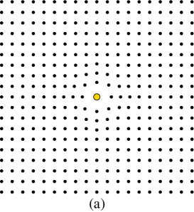
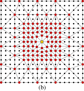
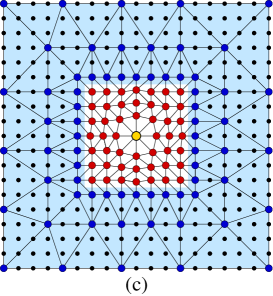
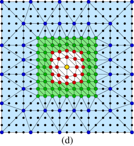
Figure 1. (a) A 2D atomistic configuration with an impurity that causes a large local deformation from the reference lattice $\varepsilon\mathbb{Z}^{2}$.   (b) Triangulation of the deformed atomistic configuration to visualize the Galerkin projection described in §2.3. The positions of the large red atoms are free, while the positions of the small black atoms are constraint by the motion of the free atoms.   (c) Visualization of the QCE method described in §2.3. The blue shaded region is the set $\Omega_{\rm c}^{\rm qce}$, the red atoms inside the white region are the set $\mathscr{L}_{\rm a}^{\rm qce}$ (both after deformation).   (d) Visualization of an interface correction as described in §2.3. The blue shaded regions is the continuum region $\Omega_{\rm c}$, the green shaded region is the interface region $\Omega_{\rm i}$, and the white region is the atomistic region $\Omega_{\rm a}$. The mesh in $\Omega_{\rm i}\cup\Omega_{\rm a}$ is chosen so that it coincides with $\mathscr{T}_{\varepsilon}$ (cf. §3.1).

Let $\Omega:=(-1,1]^{d}$, and let $\mathscr{T}_{h}$ be a regular [7] triangulation of $\bar{\Omega}$, with vertices belonging to $\mathscr{L}^{\#}$, that can be extended periodically to a regular triangulation $\mathscr{T}_{h}^{\#}$ of $\mathbb{R}^{d}$. We make the convention that elements $T\in\mathscr{T}_{h}$ are closed sets. For $T\in\mathscr{T}_{h}$ we define $h_{T}:={\rm diam}(T)$, and for each $x\in\mathbb{R}^{d}$ we define $h(x):=\max\{h_{T}\,|\,T\in\mathscr{T}_{h}\text{ s.t. }x\in T\}$.

We define the ${\rm P}_{1}$ finite element space

$${\rm P}_{1}(\mathscr{T}_{h}^{\#}):=\big{\{}v_{h}:\mathscr{L}^{\#}\to\mathbb{R}\,\big{|}\,v_{h}\text{ is piecewise affine w.r.t. }\mathscr{T}_{h}^{\#}\big{\}},$$

and we denote the spaces of piecewise affine displacements and deformations, respectively, by

$$\mathscr{U}_{h}:=\mathscr{U}\cap{\rm P}_{1}(\mathscr{T}_{h}^{\#})^{d},\quad\mathscr{Y}_{h}:=\mathscr{Y}\cap{\rm P}_{1}(\mathscr{T}_{h}^{\#})^{d},\quad\text{and}\quad\mathscr{Y}_{{\sf A},h}:=\mathscr{Y}_{\sf A}\cap{\rm P}_{1}(\mathscr{T}_{h}^{\#})^{d}.$$

For future reference, let $I_{h}:\mathscr{Y}\to\mathscr{Y}_{h}$ denote the nodal interpolation operator. We note that $I_{h}:\mathscr{Y}_{\sf A}\to\mathscr{Y}_{{\sf A},h}$ as well as $I_{h}:\mathscr{U}\to\mathscr{U}_{h}$. We also define ${\rm P}_{1}^{\#}(\mathscr{T}_{h})$ to be the set of all $2\mathbb{Z}^{d}$-periodic functions $v_{h}\in{\rm P}_{1}(\mathscr{T}_{h}^{\#})$; i.e., $\mathscr{U}_{h}={\rm P}_{1}^{\#}(\mathscr{T}_{h})^{d}$. Let $\mathscr{F}_{h}^{\#}$ denote the set of closed edges of the extended triangulation $\mathscr{T}_{h}^{\#}$, and let $\mathscr{F}_{h}$ denote the set of all edges $f\in\mathscr{F}_{h}^{\#}$ such that ${\rm area}(f\cap\Omega)\neq 0$. Finally, we introduce the spaces of piecewise constant functions ${\rm P}_{0}(\mathscr{T}_{h})$, ${\rm P}_{0}(\mathscr{T}_{h}^{\#})$, and ${\rm P}_{0}^{\#}(\mathscr{T}_{h})$, defined in a similar manner.

The Galerkin approximation of (7) is the coarse-grained minimization problem

$$y_{{\rm a},h}\in\underset{y_{h}\in\mathscr{Y}_{{\sf A},h}}{{\rm argmin}}\,\mathscr{E}_{\rm a}^{\rm tot}(y_{h}),$$ (10)

where we recall that $\mathscr{E}_{\rm a}^{\rm tot}=\mathscr{E}_{\rm a}+\mathscr{P}_{\rm a}$.

For example, if we choose the triangulation $\mathscr{T}_{h}$ as in Figure 1(b), then we obtain full atomistic resolution in the neighbourhood of the defect, while considerably reducing the overall number of degrees of freedom by coarsening the mesh away from the defect. In this way it is possible to obtain highly accurate approximations to nontrivial atomistic configurations. Under suitable technical assumptions it is not too difficult to employ the classical techniques of finite element error analysis in this context. Such analyses, including a posteriori grid generation, are given in [28, 29, 42].

Remark 1 (Regularity of Atomistic Solutions). In order for the Galerkin projection method, or the subsequent a/c coupling methods, to be accurate we require “regularity” of atomistic solutions. Such a regularity theory does not exist at present, however, most numerical experiments performed on atomistic models for simple lattices indicate “smoothness” of atomistic deformations away from defects. The situation would be different for so-called multi-lattices, which require a homogenisation step and represent a far greater challenge. ∎

Continuum region & Cauchy–Born approximation

The Galerkin projection (10) reduces the number of degrees of freedom considerably, however, the complexity of computing $\mathscr{E}_{\rm a}|_{\mathscr{Y}_{h}}$ is not reduced in the same manner. Due to the non-locality of the atomistic interaction $\mathscr{E}_{\rm a}|_{\mathscr{Y}_{h}}$ cannot be evaluated as easily as in the case of finite element methods for continuum mechanics. Several attempts have been made to use quadrature ideas to approximate $\mathscr{E}_{\rm a}$ and render (10) computationally efficient [18, 21, 24], however, it was shown in [31] that these approximations yield unacceptable consistency errors.

An alternative approach, proposed in [37], is to keep the full atomistic description for atomistically fine elements, while employing the Cauchy–Born approximation for coarser elements as well as an interface region. Following the terminology of [12] we call the resulting method the QCE method (the original energy-based quasicontinuum method).

To formulate this method we choose a set $\mathscr{L}_{\rm a}^{\rm qce}\subset\mathscr{L}$ of atoms that we wish to treat atomistically (the red atoms in Figure 1(c)). Let $Q_{\varepsilon}(x):=x+\varepsilon(-{\textstyle\frac{1}{2}},{\textstyle\frac{1}{2}}]^{d}$, and define

$$\text{and}\quad\Omega_{\rm c}^{\rm qce}:=\Omega\setminus\bigcup_{x\in\mathscr{L}_{\rm a}^{\rm qce}}Q_{\varepsilon}(x).$$

With this notation, the QCE energy functional is defined, for $y_{h}\in\mathscr{Y}_{h}$, as

$$\mathscr{E}_{\rm qce}(y_{h}):=\varepsilon^{d}\sum_{x\in\mathscr{L}_{\rm a}^{\rm qce}}V\big{(}D_{\!\mathscr{R}}y_{h}(x)\big{)}+\int_{\Omega_{\rm c}^{\rm qce}}W(\nabla y_{h})\,{\rm d}x,$$ (11)

where $W:\mathbb{R}^{d\times d}\to\mathbb{R}$ is the Cauchy–Born stored energy function,

$$W({\sf F}):=V({\sf F}\mathscr{R})=V\big{(}({\sf F}r)_{r\in\mathscr{R}}\big{)}.$$ (12)

Note that $W({\sf F})$ is the energy of a single atom in the Bravais lattice ${\sf F}\mathscr{L}^{\#}$.

One may readily check that the complexity of evaluating $\mathscr{E}_{\rm qce}$ (or its derivatives) is of the order $O(\#\mathscr{T}_{h})$, that is, of the same order as the number of degrees of freedom. Moreover, it is easy to see that $\mathscr{E}_{\rm qce}(y_{\sf A})=\mathscr{E}_{\rm a}(y_{\sf A})$ for all ${\sf A}\in\mathbb{R}^{d\times d}$. For future reference, we give a formal definition of this property.

Definition 1 (Global Energy Consistency). We say that an energy functional $\mathscr{E}\in{\rm C}(\mathscr{Y})$ is globally energy consistent if

$$\mathscr{E}(y_{\sf A})=\mathscr{E}_{\rm a}(y_{\sf A})\qquad\forall{\sf A}\in\mathbb{R}^{d\times d}.$$ (13)

More generally one can show that $\mathscr{E}_{\rm qce}(y_{h})$ is a good approximation to $\mathscr{E}_{\rm a}(y_{h})$ if $\nabla y_{h}$ varies only moderately. Despite these facts, it turns out, as we discuss in §2.3 and §4.2, that minimizers of $\mathscr{E}_{\rm qce}$ are poor approximations to minimizers of $\mathscr{E}_{\rm a}$.

Remark 2 (The Cauchy–Born Model). The Cauchy–Born model is a standard continuum model, for large deformations of single crystals. In the absence of defects, solutions of a pure Cauchy–Born model (no atomistic region) can provide excellent approximations to solutions of the atomistic model (7). For example, in [17] it is shown that, for smooth and small dead load external forces, and under realistic stability assumptions on $\mathscr{E}_{\rm a}$, there exist solutions $y_{\rm a}$ of (7) and $y_{\rm c}$ of the Cauchy–Born model, such that

$$\bigg{(}\varepsilon^{d}\sum_{x\in\mathscr{L}}\sum_{j=1}^{d}\big{|}D_{\!e_{j}}y_{\rm a}(x)-D_{\!e_{j}}{y}_{\rm c}(x)\big{|}^{2}\bigg{)}^{1/2}\leq C\varepsilon^{2},$$

where $C$ depends on higher partial derivatives of $V$ and on the regularity of ${y}_{\rm c}$. Hence, in the regime of “smooth elastic” deformations, the Cauchy–Born model can be considered an excellent approximation to the atomistic model (3). ∎

The patch test

The patch test is often employed in the theory of finite element methods [53, 6, 5] as a simple test for consistency. The test also plays an important role in the design of a/c methods.

Definition 2 (Patch Test Consistency). We say that an energy functional $\mathscr{E}\in{\rm C}^{1}(\mathscr{Y}_{h};\mathbb{R})$ is patch test consistent if it satisfies

$$\big{\langle}\delta\mathscr{E}(y_{\sf F}),u_{h}\big{\rangle}=0\qquad\forall\,u_{h}\in\mathscr{U}_{h},\quad\forall\,{\sf F}\in\mathbb{R}^{d\times d}.$$ (14)

The terminology “patch test consistency” is motivated by Proposition 2.1, where we have shown that the exact energy $\mathscr{E}_{\rm a}$ does satisfy the patch test (14).

However, the QCE energy $\mathscr{E}_{\rm qce}$ is not patch test consistent [50]. This result will be reviewed for a one-dimensional model problem in §4.2, where it will also be shown how failure of the patch test affects the consistency error.

Remark 3. In most of the a/c coupling literature the patch test is stated as the condition that

$$\frac{\partial\mathscr{E}(y_{h})}{\partial y_{h}(p)}\Big{|}_{y_{h}=y_{\sf F}}=0\quad\text{ for all finite element nodes }p.$$

It is straightforward to see that this condition is equivalent to the variational formulation given in (14). ∎

Interface correction

In the engineering literature (see, e.g., [50, 35]) the non-zero forces under homogeneous strains of patch test inconsistent a/c energies are usually dubbed “ghost forces”. The discovery that $\mathscr{E}_{\rm qce}$ is not patch test consistent has resulted in a number of works constructing new a/c methods that removed or reduced the “ghost forces” [4, 15, 49, 52, 56, 23, 27, 55, 22]. In some cases, this is achieved through sacrificing a variational (i.e., conservative, or, energy-based) formulation [10, 20, 25, 33, 46, 50, 51].

In the present paper we will focus only on energy-based a/c methods that are patch test consistent, i.e., that remove the “ghost forces” altogether. None of the methods presently available in the literature have resolved this problem in its full generality, however, [15, 49, 52, 22] present several interesting approaches and partial solutions. In the following, we present a generalization of the geometrically consistent coupling method [15], which is the most general approach but leaves some questions concerning its practical construction open.

Let $\mathscr{T}^{\rm c}_{h}\subset\mathscr{T}_{h}$ and $\Omega_{\rm c}=\cup\mathscr{T}^{\rm c}_{h}$. We assume that all atoms belonging to $\mathscr{L}\setminus{\rm int}(\Omega_{\rm c})$ are vertices of $\mathscr{T}_{h}$, and we define two sets $\mathscr{L}_{\rm a}^{\rm gc},\mathscr{L}_{\rm i}^{\rm gc}$ such that

$$\mathscr{L}_{\rm a}^{\rm gc}\cup\mathscr{L}_{\rm i}^{\rm gc}=\mathscr{L}\setminus{\rm int}(\Omega_{\rm c}),\quad\text{and}\quad\mathscr{L}_{\rm a}^{\rm gc}\cap\mathscr{L}_{\rm i}^{\rm gc}=\emptyset.$$

For each $x\in\mathscr{L}_{\rm i}^{\rm gc}$, we define a modified interaction potential $\widetilde{V}(x;\cdot)\in{\rm C}^{2}((\mathbb{R}^{d})^{\mathscr{R}})$, and we define the a/c energy functional as

$$\mathscr{E}_{\rm gc}(y_{h}):=\varepsilon^{d}\sum_{x\in\mathscr{L}_{\rm a}^{\rm gc}}V\big{(}D_{\!\mathscr{R}}y(x)\big{)}+\varepsilon^{d}\sum_{x\in\mathscr{L}_{\rm i}^{\rm gc}}\widetilde{V}\big{(}x;D_{\!\mathscr{R}}y(x)\big{)}+\int_{\Omega_{\rm c}}W(\nabla y_{h})\,{\rm d}x.$$ (15)

For the modified potential $\widetilde{V}$ one takes a general ansatz with several free parameters, which are then fitted to remove or minimize the ghost force. For example, following the ideas of the quasinonlocal coupling method [52] and the geometrically consistent coupling method [15] one may define

$$\widetilde{V}\big{(}x;{\bf g}\big{)}=V\big{(}(\tilde{g}_{r})_{r\in\mathscr{R}}\big{)},\quad\text{where}\quad\tilde{g}_{r}=\sum_{s\in\mathscr{R}}C_{x,r,s}g_{s}.$$

The constants $C_{x,r,s}$ can then be determined analytically as in [15, 44], or, as proposed in [45], numerically in a preprocessing step. The 2D numerical experiments performed in [45] suggest that it is always possible to determine parameters $C_{x,r,s}$ such that $\mathscr{E}_{\rm ac}$ becomes patch test consistent, however, a proof of this fact is still missing.

The purpose of the present work is to investigate the question whether patch test consistency is in fact a sufficient condition for first-order consistency of an a/c coupling method. If this would turn out to be false in general, then it would be necessary to develop new approaches for constructing accurate a/c methods.

General assumptions on the interface correction.

For the subsequent analysis we assume an even more general form of the a/c functional than (15). We choose $\mathscr{T}^{\rm c}_{h},\mathscr{T}^{\rm i}_{h},\mathscr{T}_{h}^{\rm a}\subset\mathscr{T}_{h}$, mutually disjoint, such that $\mathscr{T}_{h}=\mathscr{T}^{\rm c}_{h}\cup\mathscr{T}^{\rm i}_{h}\cup\mathscr{T}_{h}^{\rm a}$, and we define the continuum, interface, and atomistic regions

$$\Omega_{\rm c}:=\cup\mathscr{T}^{\rm c}_{h},\quad\Omega_{\rm i}:=\cup\mathscr{T}^{\rm i}_{h},\quad\text{and}\quad\Omega_{\rm a}:=\cup\mathscr{T}_{h}^{\rm a}.$$

(Note that $\Omega_{\rm c},\Omega_{\rm i},\Omega_{\rm a}$ are closed sets.) Next, we define the set of all nodes $\mathscr{L}_{\rm a}\subset\mathscr{L}$ that interact with the atomistic region:

$$\mathscr{L}_{\rm a}:=\Big{\{}x\in\mathscr{L}\,\Big{|}\,(x,x+\varepsilon r)\cap\Omega_{\rm a}^{\#}\neq\emptyset\text{ for some }r\in\mathscr{R}\Big{\}},$$

where the ordered pair $(x,x^{\prime})\in\mathscr{L}^{\#}\times\mathscr{L}^{\#}$ is called a bond; here, and throughout, the symbol $(x,x^{\prime})$ is also identified with the segment ${\rm conv}\{x,x^{\prime}\}$ (in particular, it is closed). To avoid interaction between $\mathscr{L}_{\rm a}$ and $\Omega_{\rm c}$, we assume throughout that

$$\big{\{}x+tr\,\big{|}\,x\in\mathscr{L}_{\rm a},t\in[0,1],r\in\mathscr{R}\big{\}}\subset\Omega_{\rm a}\cup\Omega_{\rm i}.$$ (16)

Next, we define the set of interface bonds

$$\mathscr{B}_{\rm i}:=\Big{\{}b=(x,x+\varepsilon r)\,\Big{|}\,x\in\mathscr{L},r\in\mathscr{R},(x,x+\varepsilon r)\subset\Omega_{\rm i}^{\#}\Big{\}}.$$

Finally, we define an interface functional $\mathscr{E}_{\rm i}\in{\rm C}^{2}(\mathscr{Y})$ such that

$$\mathscr{E}_{\rm i}(y)=\varepsilon^{d}E_{\rm i}\Big{(}\big{(}D_{\!r}y(x);(x,x+\varepsilon r)\in\mathscr{B}_{\rm i}\big{)}\Big{)},$$ (17)

that is, the interface functional $\mathscr{E}_{\rm i}$ is given as a function of the finite differences $D_{\!r}y(x)$ of bonds $(x,x+\varepsilon r)$ that are contained in the interface region. Note also the volumetric scaling $\varepsilon^{d}$.

With this notation, we set

$$\mathscr{E}_{\rm ac}(y_{h}):=\varepsilon^{d}\sum_{x\in\mathscr{L}_{\rm a}}V\big{(}D_{\!\mathscr{R}}y_{h}(x)\big{)}+\int_{\Omega_{\rm c}}W(\nabla y_{h})\,{\rm d}x+\mathscr{E}_{\rm i}(y_{h}).$$ (18)

The interface functional $\mathscr{E}_{\rm i}(y_{h})$ specifies the different variants of a/c methods. It is easy to see that the functionals $\mathscr{E}_{\rm qce}$ and $\mathscr{E}_{\rm gc}$, discussed above, fit this framework (in the case of $\mathscr{E}_{\rm qce}$ we have to drop the assumption (16)).

If we define the total a/c energy as $\mathscr{E}_{\rm a}^{\rm tot}:=\mathscr{E}_{\rm ac}+\mathscr{P}_{\rm ac}$, where $\mathscr{P}_{\rm ac}$ is a suitable a/c approximation to $\mathscr{P}_{\rm a}$ , the a/c approximation to (7) is

$$y_{\rm ac}\in\underset{y_{h}\in\mathscr{Y}_{{\sf A},h}}{\rm argmin}\,\mathscr{E}_{\rm ac}^{\rm tot}(y_{h}).$$ (19)

If $y_{\rm ac}$ solves (19), then it is a critical point of $\mathscr{E}_{\rm ac}^{\rm tot}=\mathscr{E}_{\rm ac}+\mathscr{P}_{\rm ac}$:

$$\big{\langle}\delta\mathscr{E}_{\rm ac}(y_{\rm ac})+\delta\mathscr{P}_{\rm ac}(y_{\rm ac}),u_{h}\big{\rangle}=0\qquad\forall u_{h}\in\mathscr{U}_{h}.$$ (20)

The locality and scaling conditions

We define notation for first and second partial derivatives of $E_{\rm i}$ as follows: for ${\bf g}=(g_{b})_{b\in\mathscr{B}_{\rm i}}$ let

$$\partial_{b}E_{\rm i}\big{(}(g_{b})_{b\in\mathscr{B}_{\rm i}}\big{)}:=\frac{\partial E_{\rm i}\big{(}(g_{b})_{b\in\mathscr{B}_{\rm i}}\big{)}}{\partial g_{b}},\quad\text{and}\quad\partial_{b}\partial_{b^{\prime}}E_{\rm i}\big{(}(g_{b})_{b\in\mathscr{B}_{\rm i}}\big{)}:=\frac{\partial^{2}E_{\rm i}\big{(}(g_{b})_{b\in\mathscr{B}_{\rm i}}\big{)}}{\partial g_{b}\partial g_{b^{\prime}}}.$$

We extend the definition periodically: if $b\in\mathscr{B}_{\rm i}$ and $\xi\in 2\mathbb{Z}^{d}$ then $\partial_{\xi+b}E_{\rm i}:=\partial_{b}E_{\rm i}$, and we make a similar definition for the second partial derivatives. In our analysis we will require two crucial properties on $E_{\rm i}$, which we call the locality and scaling conditions:

The locality condition

$$\partial_{(x,x+\varepsilon r)}\partial_{(x^{\prime},x^{\prime}+\varepsilon s)}E_{\rm i}(y)=0\qquad\begin{array}[]{l}\text{for all bonds }(x,x+\varepsilon r),(x^{\prime},x^{\prime}+\varepsilon s)\in\mathscr{B}_{\rm i}\\ \text{such that }x\neq x^{\prime},\end{array}$$ (21)

implies that the same bonds interact through $\mathscr{E}_{\rm i}$ as in the atomistic model. This condition can be weakened, by requiring that only bonds within an $O(\varepsilon)$ distance interact, however, such a more general condition would add additional notational complexity.

In the scaling condition we assume that there exist constants $M_{r,s}^{\rm i}\geq 0$, $r,s\in\mathscr{R}$, such that

$$\big{\|}\partial_{(x,x+\varepsilon r)}\partial_{(x,x+\varepsilon s)}E_{\rm i}(y)\big{\|}\leq~{}\left\{\begin{array}[]{rl}M_{r,s}^{\rm i},&\quad\forall(x,x+\varepsilon r),(x,x+\varepsilon s)\in\mathscr{B}_{\rm i},\\[5.69054pt] {\textstyle\frac{1}{2}}M_{r,s}^{\rm i},&\quad\text{if }{\rm length}\big{(}\partial\Omega_{\rm i}^{\#}\cap(x,x+\varepsilon r)\big{)}>0.\end{array}\right.$$ (22)

This condition effectively yields an $O(1)$ Lipschitz bound for $\delta\mathscr{E}_{\rm i}$ in the function spaces we will use. The scaling aspect enters through an implicit assumption on the magnitude of the constants $M_{r,s}^{\rm i}$, namely, we will assume throughout that the constant

$$M^{\rm i}:=\sum_{r\in\mathscr{R}}\sum_{s\in\mathscr{R}}|r||s|M_{r,s}^{\rm i}$$ (23)

is of the same order of magnitude as the constant $M^{\rm a}$ defined in (6).

Remark 4. The factor ${\textstyle\frac{1}{2}}$ for bonds on the boundary of the interface region is not strictly necessary, since it can be removed by simply replacing $M_{r,s}^{\rm i}$ with $2M_{r,s}^{\rm i}$, however, if stated as above it makes the statements of the results in §6 slightly sharper, and moreover simplifies the argument in (68).

The necessity of this factor is related to the fact that we allow $E_{\rm i}$ to depend on bonds that lie on the boundary of $\Omega_{\rm i}^{\#}$; this is made clear in Proposition 6.2 where we construct a stress function for $\mathscr{E}_{\rm ac}$. Note that if we did not allow $E_{\rm i}$ to depend on these boundary bonds, then it would in fact be impossible to construct patch test consistent a/c methods for non-flat a/c interfaces. ∎

3. A Framework for the a priori Error Analysis of a/c Methods

When analyzing the error of a numerical method, one should first of all determine the main quantities of interest. For a/c methods, one is usually interested in energy differences between homogeneous lattices and lattices with defects, or critical loads at which defects form or move (i.e., bifurcation points). Since the present paper is mostly theoretical, we will simply focus on the error in the deformation gradient. We note, however, that many aspects of this analysis are crucial ingredients for the analysis of energy differences (see, e.g., [41]) and would usually also enter an analysis of bifurcation points.

We assume from now on that $d\in\{1,2\}$. To execute the abstract framework of this section also in 3D, several technical tools as well as the central consistency result need to be developed first.

3.1. Discrete and continuous functions

In the following analysis it will be important to extend the a/c functional $\mathscr{E}_{\rm ac}$ to all functions $y\in\mathscr{Y}$. To that end, we first define piecewise affine interpolants with respect to an atomistic mesh $\mathscr{T}_{\varepsilon}$.

We take a subdivision of the scaled unit cube $\varepsilon(0,1)^{d}$ into $d$-simplices (in 1D the interval $\varepsilon(0,1)$; in 2D two symmetric triangles; compare with the triangulation of the atomistic region in Figure 1(d)), which we extend periodically to a triangulation $\mathscr{T}_{\varepsilon}^{\#}$ of $\mathbb{R}^{2}$ with vertex set $\mathscr{L}^{\#}$. The restriction of $\mathscr{T}_{\varepsilon}^{\#}$ to $\Omega$ is denoted by $\mathscr{T}_{\varepsilon}$. Each discrete function $v:\mathscr{L}^{\#}\to\mathbb{R}^{k}$ will from now on be identified in a canonical way with its continuous piecewise affine interpolant $v\in{\rm P}_{1}(\mathscr{T}_{\varepsilon}^{\#})^{k}$.

For future reference we denote the sets of edges of $\mathscr{T}_{\varepsilon}$ and $\mathscr{T}_{\varepsilon}^{\#}$, corresponding to the definitions of $\mathscr{F}_{h}$ and $\mathscr{F}_{h}^{\#}$ in §2.3, by $\mathscr{F}_{\varepsilon}$ and $\mathscr{F}_{\varepsilon}^{\#}$.

Ambiguity of continuous interpolants

If $y_{h}\in\mathscr{Y}_{h}$ then $y_{h}$ can also be interpreted as a member of $\mathscr{Y}$ and therefore has two, possibly different, continuous interpolants. To distinguish them, we make the convention that the symbol $y_{h}$ always denotes the interpolant in ${\rm P}_{1}(\mathscr{T}_{h})^{d}$, while a symbol $y$ always denotes the interpolant in ${\rm P}_{1}(\mathscr{T}_{\varepsilon})^{d}$. If we wish to evaluate the ${\rm P}_{1}(\mathscr{T}_{\varepsilon})^{d}$-interpolant of a function $y_{h}\in\mathscr{Y}_{h}$ then we will write $I_{\varepsilon}y_{h}$.

To compare a ${\rm P}_{1}(\mathscr{T}_{\varepsilon})^{d}$-interpolant with a ${\rm P}_{1}(\mathscr{T}_{h})^{d}$-interpolant, we use the following lemma. In 1D the result is easy to establish; in 2D it depends on a technical tool that we introduce in §5.1. The proof is given in the appendix.

Lemma 2. Let $d\in\{1,2\}$; then, for all $y_{h}\in\mathscr{Y}_{h}$ and $p\in[1,\infty]$, we have

$$\|\nabla I_{\varepsilon}y_{h}\|_{{\rm L}^{p}(\Omega)}\leq\|\nabla y_{h}\|_{{\rm L}^{p}(\Omega)},$$

where we recall that we have defined $\|\nabla v\|_{{\rm L}^{p}}=\|\,|\nabla v|_{p}\|_{{\rm L}^{p}}$.

Extension of the a/c energy

Before we extend the a/c energy $\mathscr{E}_{\rm ac}$ we make one last technical assumption, which considerably simplifies the subsequent analysis. We shall assume from now on, that

$$\mathscr{T}_{h}^{\rm a}\cup\mathscr{T}^{\rm i}_{h}\subset\mathscr{T}_{\varepsilon}.$$

If all atoms in $\mathscr{L}\cap(\Omega_{\rm a}\cup\Omega_{\rm i})$ are vertices of $\mathscr{T}_{h}^{\rm a}\cup\mathscr{T}^{\rm i}_{h}$, which is not uncommon, then this is no restriction.

With these conventions the a/c energy $\mathscr{E}_{\rm ac}$ defined in (18) can be defined canonically for functions $\tilde{y}=y+u_{h}\in\mathscr{Y}+\mathscr{U}_{h}$ by the same formula:

$$\mathscr{E}_{\rm ac}(\tilde{y})=\int_{\Omega_{\rm c}}W(\nabla\tilde{y})\,{\rm d}x+\varepsilon^{d}\sum_{x\in\mathscr{L}_{\rm a}}V\big{(}D_{\!\mathscr{R}}\tilde{y}(x)\big{)}+\mathscr{E}_{\rm i}(\tilde{y})\qquad\text{for }\tilde{y}\in\mathscr{Y}+\mathscr{U}_{h}.$$

We also assume that $\mathscr{P}_{\rm ac}$ has a suitable extension to $\mathscr{Y}$. It should be stressed that for general $y_{h}\in\mathscr{Y}_{h}$, $\mathscr{E}_{\rm ac}(y_{h})\neq\mathscr{E}_{\rm ac}(I_{\varepsilon}y_{h})$.

3.2. Measuring smoothness; An interpolation error estimate

The three main ingredients in the a priori error analysis of Galerkin-like approximations are (i) consistency, (ii) stability, and (iii) an interpolation error estimate. We begin by establishing the latter. To that end, we first need to find a convenient measure of smoothness for discrete functions $y\in\mathscr{Y}$.

Measuring smoothness in terms of local oscillation

There are several possibilities to measure the “smoothness” of a discrete function. The most obvious is possibly the use of higher order finite differences, e.g., $D_{\!e_{i}}D_{\!e_{j}}y(x)$. If, in §3.1, we had chosen continuous interpolants belonging to ${\rm W}^{2,\infty}$, then we would be able to simply evaluate the second derivatives $\nabla^{2}y$. However, since the interpolants we use are piecewise affine, the second derivative of $y$ is the measure $[\![\nabla y]\!]\otimes\nu\,{\rm d}s\big{|}_{\mathscr{F}_{\varepsilon}^{\#}}$, where $[\![\nabla y]\!]$ denotes the jump of $\nabla y$ across an element edge, and $\,{\rm d}s$ the surface measure.

This last observation motivates the idea to measure smoothness of $y$ by the local oscillation of $\nabla y$. We define the oscillation operator, for measurable sets $\omega\subset\mathbb{R}^{d}$, and for $y\in\mathscr{Y}$, as

$${\rm osc}(\nabla y;\omega):=\underset{x,x^{\prime}\in\omega}{\rm ess~{}sup}\,\frac{\big{|}\nabla y(x)-\nabla y(x^{\prime})\big{|}}{\varepsilon}.$$ (24)

The sets $\omega$ that arise naturally in our analysis will always have $O(\varepsilon)$ diameter, which is the reason for the $\varepsilon^{-1}$-scaling in the definition of ${\rm osc}$.

Note, in particular, that if $y$ were twice differentiable, and if ${\rm diam}(\omega)\leq C\varepsilon$, then we would obtain

$${\rm osc}(\nabla y;\omega)\leq\frac{{\rm diam}(\omega)}{\varepsilon}\,\|\nabla^{2}y\|_{{\rm L}^{\infty}(\omega)}\leq C\|\nabla^{2}y\|_{{\rm L}^{\infty}(\omega)},$$

which further illustrates that the oscillation operator is a reasonable replacement for $\nabla^{2}y$ to measure the local smoothness of a piecewise affine function.

Interpolation error estimate

The smoothness measure we defined in §3.2 yields a simple proof of an interpolation error estimate; see Appendix A.

Lemma 3. Let $d\in\{1,2\}$ and suppose that $\mathscr{T}_{h}^{\rm a}\cup\mathscr{T}^{\rm i}_{h}\subset\mathscr{T}_{\varepsilon}$; then there exists a constant $C_{I}$, which depends only on the shape regularity of $\mathscr{T}_{h}$, such that, for all $y\in\mathscr{Y}$, $p\in[1,\infty)$,

$$\big{\|}\nabla(y-I_{h}y)\big{\|}_{{\rm L}^{p}(\Omega)}\leq C_{I}\bigg{\{}\sum_{T\in\mathscr{T}_{\varepsilon}^{\rm c}}|T|\Big{[}{\rm h}_{T}\,{\rm osc}(\nabla y;\omega_{T}^{\rm c})\Big{]}^{p}\bigg{\}}^{1/p},$$

where, for $T\in\mathscr{T}_{\varepsilon}$,

$$\omega_{T}^{\rm c}:=\Omega_{\rm c}^{\#}\cap\bigcup\big{\{}T^{\prime}\in\mathscr{T}_{\varepsilon}^{\#}\,\big{|}\,T\cap T^{\prime}\neq\emptyset\big{\}},\quad\text{and}\quad{\rm h}_{T}:=\max_{x\in T}|h(x)|.$$ (25)

Similarly, for $p=\infty$, we have $\big{\|}\nabla(y-I_{h}y)\big{\|}_{{\rm L}^{\infty}(\Omega)}\leq C_{I}\max_{T\in\mathscr{T}_{\varepsilon}^{\rm c}}\big{[}{\rm h}_{T}\,{\rm osc}(\nabla y;\omega_{T}^{\rm c})\big{]}$.

3.3. The stability assumption

The stability of a/c methods relies, firstly, on the stability of atomistic models as well as their Cauchy–Born approximations. It requires a thorough understanding of the physics of a model and in particular more specific information about the interaction potential. Since the focus of the present work is the consistency of a/c methods, we will formulate stability as an assumption.

The simplest notion of stability one may use, which is also closely connected to local minimality, is coercivity of the second variation:

$$\langle\delta^{2}\mathscr{E}_{\rm ac}^{\rm tot}(y_{h})u_{h},u_{h}\rangle\geq c_{0}\|\nabla u_{h}\|_{{\rm L}^{2}(\Omega)}^{2}\qquad\forall\,u_{h}\in\mathscr{U}_{h},$$ (26)

where $c_{0}>0$, and $y_{h}\in\mathscr{Y}_{h}$ is a suitable deformation in a neighbourhood of the atomistic solution $y_{\rm a}$, e.g., $y_{h}=I_{h}y_{\rm a}$. The choice of norm is motivated by the fact that the Cauchy–Born model, and hence the atomistic model, are closely related to second order elliptic differential equations.

Examples of sharp stability estimates for a/c methods in 1D can be found in [13, 40, 27, 26, 55]. For pair interactions in 2D the stability of Shapeev’s method [49] is established in [41].

More generally, for some $p\in[1,\infty],p^{\prime}=p/(p-1)$, we may assume an inf-sup condition of the form

$$\inf_{\begin{subarray}{c}u_{h}\in\mathscr{U}_{h}\\ \|\nabla u_{h}\|_{{\rm L}^{p}(\Omega)}=1\end{subarray}}\sup_{\begin{subarray}{c}v_{h}\in\mathscr{U}_{h}\\ \|\nabla v_{h}\|_{{\rm L}^{p^{\prime}}(\Omega)}=1\end{subarray}}\big{\langle}\delta^{2}\mathscr{E}_{\rm ac}^{\rm tot}(y_{h})u_{h},v_{h}\big{\rangle}\geq c_{0},$$ (27)

for some constant $c_{0}>0$. The condition (27) is usually difficult to prove, especially for $p\neq 2$, and may indeed be false in general. We will only use it to demonstrate how such a stability result motivates consistency estimates in different negative norms. Examples of 1D inf-sup stability estimates for a/c methods can be found in [10, 14, 32, 42].

3.4. Outline of an a priori error analysis

The following outline of an a priori error analysis depends on a stability assumption that we will not prove. Moreover, since it primarily serves to motivate the consistency problem, and since a rigorous derivation would be more involved without yielding much additional insight, some steps will be kept vague. Most of these steps are easily made rigorous; the main assumption we make below, which is in fact very difficult to justify rigorously, is that $I_{h}y_{\rm a}$ and $y_{\rm ac}$ are “sufficiently close”. See [32, 40, 42, 55] for similar analyses in 1D where all steps are rigorously justified, and [43, 41] for a similar semi-rigorous framework, where a proof of this step is replaced by an assumption.

Let $y_{\rm a}$ satisfy (8), $y_{\rm ac}$ satisfy (20), and suppose that the stability assumption (27) holds with $y_{h}=I_{h}y_{\rm a}$. Let $e_{h}:=y_{\rm ac}-I_{h}y_{\rm a}$. Moreover, suppose that $\|\nabla I_{h}y_{\rm a}-\nabla y_{\rm ac}\|_{{\rm L}^{\infty}}$ is sufficiently small so that the following approximation can be made precise:

$$\big{<}\delta^{2}\mathscr{E}_{\rm ac}^{\rm tot}(I_{h}y_{\rm a})e_{h},v_{h}\big{\rangle}\approx~{} \int_{0}^{1}\big{\langle}\delta^{2}\mathscr{E}_{\rm ac}^{\rm tot}(I_{h}y_{\rm a}+te_{h})e_{h},v_{h}\big{\rangle}\,{\rm d}t$$

$$=~{} \big{\langle}\delta(\mathscr{E}_{\rm ac}+\mathscr{P}_{\rm ac})(y_{\rm ac})-\delta(\mathscr{E}_{\rm ac}+\mathscr{P}_{\rm ac})(I_{h}y_{\rm a}),v_{h}\big{\rangle}.$$

Taking the supremum over all $v_{h}\in\mathscr{U}_{h}$, and invoking the inf-sup condition (27) and the criticality condition (20), we obtain

$$c_{0}\big{\|}\nabla e_{h}\big{\|}_{{\rm L}^{p}(\Omega)}\lesssim\big{\|}\delta(\mathscr{E}_{\rm ac}+\mathscr{P}_{\rm ac})(I_{h}y_{\rm a})\big{\|}_{{\rm W}^{-1,p}_{h}},$$

where we define

$$\|\Phi\|_{{\rm W}^{-1,p}_{h}}:=\sup_{\begin{subarray}{c}v_{h}\in\mathscr{U}_{h}\\ \|\nabla v_{h}\|_{{\rm L}^{p^{\prime}}}=1\end{subarray}}\big{\langle}\Phi,v_{h}\big{\rangle},\qquad\text{for }\Phi\in\mathscr{U}_{h}^{*}.$$

We split the consistency error $\|\delta(\mathscr{E}_{\rm ac}+\mathscr{P}_{\rm ac})(I_{h}y_{\rm a})\|_{{\rm W}^{-1,p}_{h}}$ into three separate contributions:

$$c_{0}\big{\|}\nabla e_{h}\big{\|}_{{\rm L}^{p}(\Omega)}\lesssim~{} \big{\|}\delta(\mathscr{E}_{\rm ac}+\mathscr{P}_{\rm ac})(I_{h}y_{\rm a})-\delta(\mathscr{E}_{\rm ac}+\mathscr{P}_{\rm ac})(y_{\rm a})\big{\|}_{{\rm W}^{-1,p}_{h}}$$

$$+\big{\|}\delta\mathscr{E}_{\rm ac}(y_{\rm a})-\delta\mathscr{E}_{\rm a}(y_{\rm a})\big{\|}_{{\rm W}^{-1,p}_{h}}+\big{\|}\delta\mathscr{P}_{\rm ac}(y_{\rm a})-\delta\mathscr{P}_{\rm a}(y_{\rm a})\big{\|}_{{\rm W}^{-1,p}_{h}}$$

$$=:~{} \mathcal{E}^{\rm coarse}_{h}+\mathcal{E}^{\rm model}_{h}+\mathcal{E}^{\rm ext}_{h}.$$ (28)

where we have used (8), and the extension of $\mathscr{E}_{\rm ac}$ and $\mathscr{P}_{\rm ac}$ for all deformations $y\in\mathscr{Y}$ constructed in §3.1.

The coarsening error, $\mathcal{E}^{\rm coarse}_{h}$, can be bounded by Lipschitz estimates for $\delta(\mathscr{E}_{\rm ac}+\mathscr{P}_{\rm ac})$ and an interpolation error estimate. Using our assumption that $\mathscr{T}_{h}^{\rm a}\cup\mathscr{T}^{\rm i}_{h}\subset\mathscr{T}_{\varepsilon}$ it is not difficult to derive Lipschitz estimates of the form

$$\mathcal{E}^{\rm coarse}_{h}\leq(M^{\rm a}+M_{\mathscr{P}_{\rm ac}})\big{\|}\nabla I_{h}y_{\rm a}-\nabla y_{\rm a}\big{\|}_{{\rm L}^{p}(\Omega)},$$ (29)

where $M^{\rm a}$ is a Lipschitz constant for $\partial W$ (cf. (12)), and $M_{\mathscr{P}_{\rm ac}}$ is a Lipschitz constant for $\delta\mathscr{P}_{\rm ac}$.

Combining (28), and (29), the inequality

$$\big{\|}\nabla y_{\rm a}-\nabla y_{\rm ac}\big{\|}_{{\rm L}^{p}}\leq\big{\|}\nabla y_{\rm a}-\nabla I_{h}y_{\rm a}\big{\|}_{{\rm L}^{p}}+\big{\|}\nabla e_{h}\big{\|}_{{\rm L}^{p}},$$

and the interpolation error estimate of Lemma 3.2, we arrive at the following basic error estimate

$$\big{\|}\nabla y_{\rm a}-\nabla y_{\rm ac}\big{\|}_{{\rm L}^{p}(\Omega)}\leq\frac{\mathcal{E}^{\rm model}_{h}+\mathcal{E}^{\rm ext}_{h}}{c_{0}}+\frac{c_{1}}{c_{0}}\bigg{\{}\sum_{T\in\mathscr{T}_{\varepsilon}^{\rm c}}\Big{[}{\rm h}_{T}\,{\rm osc}(\nabla y_{\rm a};\omega_{T}^{\rm c})\Big{]}^{p}\bigg{\}}^{1/p},$$ (30)

where $c_{1}=C_{I}(c_{0}+M^{\rm a}+M_{\mathscr{P}_{\rm ac}})$.

The consistency error for the external forces, $\mathcal{E}^{\rm ext}_{h}$, depends on the form of $\mathscr{P}_{\rm a}$ and $\mathscr{P}_{\rm ac}$ and cannot be discussed at this level of abstraction. The modelling error, $\mathcal{E}^{\rm model}_{h}$, is the focus of the remainder of the present paper.

Remark 5 (Choice of Splitting). Suppose, for simpliciy, that $\mathscr{P}_{\rm ac}=\mathscr{P}_{\rm a}=0$. In a typical finite element error analysis of continuum mechanics problems one would usually choose a different splitting of the consistency error:

$$\big{\|}\delta\mathscr{E}_{\rm ac}(I_{h}y_{\rm a})\big{\|}_{{\rm W}^{-1,p}_{h}}\leq\big{\|}\delta\mathscr{E}_{\rm ac}(I_{h}y_{\rm a})-\delta\mathscr{E}_{\rm a}(I_{h}y_{\rm a})\big{\|}_{{\rm W}^{-1,p}_{h}}+\big{\|}\delta\mathscr{E}_{\rm a}(I_{h}y_{\rm a})-\delta\mathscr{E}_{\rm a}(y_{\rm a})\big{\|}_{{\rm W}^{-1,p}_{h}}.$$

This splitting was used in the analysis in [41] and led to a suboptimal estimate of the modelling error, since it still contains some coarsening error. ∎

3.5. The consistency problem

The main step that remains in obtaining an a priori error estimate from (30) is the estimation of the modelling error

$$\mathcal{E}^{\rm model}_{h}=\big{\|}\delta\mathscr{E}_{\rm ac}(y_{\rm a})-\delta\mathscr{E}_{\rm a}(y_{\rm a})\big{\|}_{{\rm W}^{-1,p}_{h}}=\sup_{\begin{subarray}{c}v_{h}\in\mathscr{U}_{h}\setminus\{0\}\end{subarray}}\frac{\big{\langle}\delta\mathscr{E}_{\rm ac}(y_{\rm a})-\delta\mathscr{E}_{\rm a}(y_{\rm a}),v_{h}\big{\rangle}}{\|\nabla v_{h}\|_{{\rm L}^{p^{\prime}}(\Omega)}}.$$

Most of the numerical analysis literature on a/c methods estimates this modelling error only for the case when $\mathscr{T}_{h}=\mathscr{T}_{\varepsilon}$. In 1D it is easy to see that this is sufficient, since $I_{\varepsilon}v_{h}=v_{h}$ in that case; see also [43]. The following lemma provides the main technical step to explain why it is also sufficient in 2D to consider the case $\mathscr{T}_{h}=\mathscr{T}_{\varepsilon}$. Its proof uses arguments similar to those in the a posteriori error analysis of continuum finite element methods and is given in Appendix A.

Lemma 4. Assume that $\mathscr{T}^{\rm i}_{h}\cup\mathscr{T}_{h}^{\rm a}\subset\mathscr{T}_{\varepsilon}$. Let $\Phi\in\mathscr{U}^{*}$ and $\Phi_{h}\in\mathscr{U}_{h}^{*}$ be given in the form

$$\big{\langle}\Phi,u\big{\rangle}=\int_{\Omega_{\rm c}}\sigma:\nabla u\,{\rm d}x,\quad\text{and}\quad\langle\Phi_{h},u_{h}\big{\rangle}=\int_{\Omega_{\rm c}}\sigma:\nabla u_{h}\,{\rm d}x,$$

for all $u\in\mathscr{U}$, $u_{h}\in\mathscr{U}_{h}$, where $\sigma\in{\rm P}_{0}^{\#}(\mathscr{T}_{\varepsilon})^{d\times d}$; then there exists a universal constant $C_{M}$ such that, for all $p\in[1,\infty)$,

$$\begin{split}\Big{|}\big{\langle}\Phi,I_{\varepsilon}u_{h}\big{\rangle}-\big{\langle}\Phi_{h},u_{h}\big{\rangle}\Big{|}\leq~{}&C_{M}\varepsilon\,\bigg{(}\sum_{T\in\mathscr{T}_{\varepsilon}^{\rm c}}|T|{\rm osc}(\sigma;\omega_{T}^{\rm c})^{p}\bigg{)}^{1/p}\big{\|}\nabla u_{h}\big{\|}_{{\rm L}^{p^{\prime}}(\Omega_{\rm c})},\quad\text{and}\\ \Big{|}\big{\langle}\Phi,I_{\varepsilon}u_{h}\big{\rangle}-\big{\langle}\Phi_{h},u_{h}\big{\rangle}\Big{|}\leq~{}&C_{M}\varepsilon\,\big{[}\max_{T\in\mathscr{T}_{\varepsilon}^{\rm c}}{\rm osc}(\sigma;\omega_{T}^{\rm c})\big{]}\,\big{\|}\nabla u_{h}\big{\|}_{{\rm L}^{1}(\Omega_{\rm c})}.\end{split}$$ (31)

The estimate (31), together with Lemma 3.1, implies the following theorem, where we use the notation

$$\|\Phi\|_{{\rm W}^{-1,p}_{\varepsilon}}:=\sup_{\begin{subarray}{c}v\in\mathscr{U}\setminus\{0\}\\ \|\nabla v\|_{{\rm L}^{p^{\prime}}}=1\end{subarray}}\big{\langle}\Phi,v\big{\rangle}\qquad\text{for }\Phi\in\mathscr{U}^{*}.$$ (32)

Theorem 5. Suppose that $\mathscr{T}_{h}^{\rm a}\cup\mathscr{T}^{\rm i}_{h}\subset\mathscr{T}_{\varepsilon}$ and that $y\in\mathscr{Y}$; then, for all $p\in[1,\infty)$,

$$\begin{split}\big{\|}\delta\mathscr{E}_{\rm ac}(y)-\delta\mathscr{E}_{\rm a}(y)\big{\|}_{{\rm W}^{-1,p}_{h}}\leq~{}&M^{\rm a}C_{M}\varepsilon\bigg{(}\sum_{T\in\mathscr{T}_{\varepsilon}^{\rm c}}|T|{\rm osc}(\nabla y(T);\omega_{T}^{\rm c})^{p}\bigg{)}^{1/p}\\ &+\big{\|}\delta\mathscr{E}_{\rm ac}(y)-\delta\mathscr{E}_{\rm a}(y)\big{\|}_{{\rm W}^{-1,p}_{\varepsilon}},\end{split}$$ (33)

with corresponding statement for $p=\infty$.

Proof.

Since $\mathscr{E}_{\rm a}(I_{\varepsilon}y_{h})$ uses only point values of $I_{\varepsilon}y_{h}$, which are the same as for $y_{h}$, we have

$$\langle\delta\mathscr{E}_{\rm a}(y),u_{h}\rangle=\langle\delta\mathscr{E}_{\rm a}(y),I_{\varepsilon}u_{h}\rangle\qquad\forall\,u_{h}\in\mathscr{U}_{h}.$$

Using this fact, we can estimate

$$\big{|}\big{\langle}\delta\mathscr{E}_{\rm ac}(y)-\delta\mathscr{E}_{\rm a}(y),u_{h}\big{\rangle}\big{|}\leq\big{|}\big{\langle}\delta\mathscr{E}_{\rm ac}(y),u_{h}\big{\rangle}-\big{\langle}\delta\mathscr{E}_{\rm ac}(y),I_{\varepsilon}u_{h}\big{\rangle}\big{|}+\big{|}\langle\delta\mathscr{E}_{\rm ac}(y)-\delta\mathscr{E}_{\rm a}(y),I_{\varepsilon}u_{h}\big{\rangle}\big{|}.$$

Due to the assumption that $\mathscr{T}_{h}^{\rm a}\cup\mathscr{T}^{\rm c}_{h}\subset\mathscr{T}_{\varepsilon}$, the first group can be estimated using Lemma 3.5, with $\sigma=\partial W(\nabla y)$, which yields the first term in (33).

Using Lemma 3.1, the second group can be estimated by

$$\big{|}\langle\delta\mathscr{E}_{\rm ac}(y)-\delta\mathscr{E}_{\rm a}(y),I_{\varepsilon}u_{h}\big{\rangle}\big{|}\leq~{} \big{\|}\delta\mathscr{E}_{\rm ac}(y)-\delta\mathscr{E}_{\rm a}(y)\big{\|}_{{\rm W}^{-1,p}_{\varepsilon}}\big{\|}\nabla I_{\varepsilon}u_{h}\big{\|}_{{\rm L}^{p^{\prime}}}$$

$$\leq~{} \big{\|}\delta\mathscr{E}_{\rm ac}(y)-\delta\mathscr{E}_{\rm a}(y)\big{\|}_{{\rm W}^{-1,p}_{\varepsilon}}\big{\|}\nabla u_{h}\big{\|}_{{\rm L}^{p^{\prime}}}.$$

Taking the supremum over all $u_{h}\in\mathscr{U}_{h}$ with $\|\nabla u_{h}\|_{{\rm L}^{p^{\prime}}}=1$ yields the stated result. ∎

Applying Theorem 3.5 to the modelling error $\mathcal{E}^{\rm model}_{h}$, defined in (28), we obtain that

$$\mathcal{E}^{\rm model}_{h}\leq\mathcal{E}^{\rm model}_{\varepsilon}+M^{\rm a}C_{M}\varepsilon\bigg{(}\sum_{T\in\mathscr{T}_{\varepsilon}^{\rm c}}|T|{\rm osc}(\nabla y(T);\omega_{T}^{\rm c})^{p}\bigg{)}^{1/p},$$ (34)

where

$$\mathcal{E}^{\rm model}_{\varepsilon}:=\big{\|}\delta\mathscr{E}_{\rm ac}(y_{\rm a})-\delta\mathscr{E}_{\rm a}(y_{\rm a})\big{\|}_{{\rm W}^{-1,p}_{\varepsilon}}.$$

Even though $\mathcal{E}^{\rm model}_{\varepsilon}$ is essentially an upper bound for $\mathcal{E}^{\rm model}_{h}$, it is usually easier to estimate. The consistency problem is to prove a sharp upper bound on $\mathcal{E}^{\rm model}_{\varepsilon}$.

In §4 we will discuss two simple 1D examples to determine what can be expected in more general situations. In Theorem 6 we will prove that for an a/c method that is patch test consistent, and satisfies various other technical conditions, one obtains

$$\mathcal{E}^{\rm model}_{\varepsilon}\leq C\,\varepsilon\,\bigg{\{}\sum_{T\in\mathscr{T}_{\varepsilon}^{\rm c}\cup\mathscr{T}_{\varepsilon}^{\rm i}}|T|\big{[}{\rm osc}(\nabla y_{\rm a};\omega_{T})\big{]}^{p}\bigg{\}}^{1/p},$$

where $C$ is a constant that is independent of $y_{\rm a}$, but does depend on the interface width, and $\omega_{T}\subset\Omega_{\rm c}\cup\Omega_{\rm i}$ is the interaction neighbourhood defined in (43).

Combined with (34) and (30), and using the fact that $\varepsilon\leq{\rm h}_{T}$, and that $\omega_{T}\supset\omega_{T}^{\rm c}$ for $T\in\mathscr{T}_{\varepsilon}^{\rm c}$, this bound yields

$$\big{\|}\nabla y_{\rm a}-\nabla y_{{\rm ac}}\big{\|}_{{\rm L}^{p}}\leq\frac{\mathcal{E}^{\rm ext}_{h}}{c_{0}}+\frac{c_{2}}{c_{0}}\bigg{\{}\sum_{T\in\mathscr{T}_{\varepsilon}^{\rm c}\cup\mathscr{T}_{\varepsilon}^{\rm i}}|T|\Big{[}{\rm h}_{T}\,{\rm osc}(\nabla y_{\rm a};\omega_{T})\Big{]}^{p}\bigg{\}}^{1/p},$$ (35)

where $c_{2}$ is a constant that is independent of $y_{\rm a}$. This estimate closely resembles a typical first-order a priori error estimate for a continuum mechanics finite element approximation; see also the interpretation given in §1.2.

It should be stressed again that (35) is not a rigorous error estimate, but depends on various assumptions made in the forgoing discussion, most prominently, the stability assumption (27), and the assumption that $\|\nabla I_{h}y_{\rm a}-\nabla y_{\rm ac}\|_{{\rm L}^{\infty}}$ is “sufficiently small”.

Remark 6. The locality of the patches $\omega_{T}$ is crucial. If ${\rm diam}(\omega_{T})$ is not of the order $O(\varepsilon)$, then it is possible that ${\rm osc}(\nabla y_{\rm a};\omega_{T})\gg 1$ even if $y_{\rm a}$ is globally smooth; see also §6.4. ∎

4. Examples in 1D

In the present section we review the consistency analyses of specific a/c methods to point out the main features and to motivate what may be expected in the general case. Throughout this section we assume that $d=1$, $\mathscr{R}=\{\pm 1,\pm 2\}$, and that $V$ is given by

$$V(\{g_{\pm 1},g_{\pm 2}\})={\textstyle\frac{1}{2}}\big{[}\phi_{1}(g_{1})+\phi_{1}(g_{-1})+\phi_{2}(g_{2})+\phi_{2}(g_{-2})\big{]},$$

where $\phi_{1},\phi_{2}\in{\rm C}^{2,1}(\mathbb{R})$ are, respectively, the first and second neighour interaction potentials, which are assumed to be symmetric about the origin. We assume that their derivatives $\phi_{i}^{\prime}$ and $\phi_{i}^{\prime\prime}$ have global Lipschitz constants $m_{i}^{\prime}$ and $m_{i}^{\prime\prime}$.

For the 1D analysis it is convenient to write $x_{n}=n\varepsilon$, $v_{n}=v(x_{n})$, and to write all interactions in terms of the backward difference operator

$$v^{\prime}_{n}=\frac{v_{n}-v_{n-1}}{\varepsilon}.$$

With this notation the atomistic energy can now be rewritten in the form

$$\mathscr{E}_{\rm a}(y)=\varepsilon\sum_{n=-N+1}^{N}\phi_{1}(y_{n}^{\prime})+\varepsilon\sum_{n=-N+1}^{N}\phi_{2}(y_{n}^{\prime}+y_{n+1}^{\prime}),$$ (36)

where we note that $y_{n}^{\prime}+y_{n+1}^{\prime}=\varepsilon^{-1}(y_{n+1}-y_{n-1})$ describes a second neighbour bond.

For future reference we also define the second and third finite differences

$$v_{n}^{\prime\prime}=\frac{v_{n+1}^{\prime}-v_{n}^{\prime}}{\varepsilon},\quad\text{and}\quad v_{n}^{\prime\prime\prime}(x)=\frac{v_{n+1}^{\prime}-2v_{n}^{\prime}+v_{n-1}^{\prime}}{\varepsilon^{2}}.$$

It is also worth pointing out that $v_{n}^{\prime}=\nabla v(s)$ for all $s\in(x_{n-1},x_{n})$.

4.1. Consistency of the QNL method

We begin with a modelling error analysis for the quasinonlocal coupling method (QNL method) of Shimokawa et al [52]. The geometrically consistent coupling scheme [15] and the method proposed by Shapeev [49] reduce to the same method for 1D second neighbour interactions.

The following presentation follows largely [40], where the QNL method is defined as follows: Let $\mathscr{N}_{\rm a}=\{-K,\dots,K\}$ for some $K\geq 1$ and $\mathscr{N}_{\rm c}=\{-N+1,\dots,N\}\setminus\mathscr{N}_{\rm a}$; then, for $y\in\mathscr{Y}$, the QNL energy is defined by

$$\begin{split}\mathscr{E}_{\rm qnl}(y)=\varepsilon\sum_{n=-N+1}^{N}\phi_{1}(y_{n}^{\prime})~{}&+\varepsilon\sum_{n\in\mathscr{N}_{\rm a}}\phi_{2}(y_{n}^{\prime}+y_{n+1}^{\prime})+\varepsilon\sum_{n\in\mathscr{N}_{\rm c}}{\textstyle\frac{1}{2}}\big{[}\phi_{2}(2y_{n}^{\prime})+\phi_{2}(2y_{n+1}^{\prime})\big{]}.\end{split}$$ (37)

We observe that we have not modified the first neighbour interactions, but have “split” the non-local second neighbour interactions into local first neighbour interactions in the continuum region.

It is straightforward to rewrite $\mathscr{E}_{\rm qnl}$ in the form specified in (18), with

$$\Omega_{\rm c}=[\varepsilon(K+1),1]\cup(-1,\varepsilon(-K-1)],\quad\mathscr{L}_{\rm a}=\varepsilon\{-K+1,\dots,K-1\},$$

and a suitably defined interface functional $\mathscr{E}_{\rm i}$; however, the form (37) is more convenient for the analysis.

The following modelling error estimate was first established in [40, Thm. 3.1]. Dobson and Luskin [12] treated a quadratic interaction case, using entirely different analytical techniques that gave an even more detailed analysis of the error; Ming and Yang [36] used related methods as [40, Thm. 3.1], but gave a qualitatively less precise estimate of consistency error. An extension of the result to linear finite range pair interactions is given in [27].

Note also that it is shown in [12] that the consistency error of the QNL method in $\ell^{p}_{\varepsilon}$-norms is of the order $O(1)$, that is, the usage of negative norms cannot be avoided.

We will discuss the estimate in detail in §4.3. The proof of the following result serves as a first guidance on how one may approach proofs of consistency of a/c methods in more general situations.

Proposition 6 (Consistency of the QNL Method). Let $y\in\mathscr{Y};$ then

$$\big{\|}\delta\mathscr{E}_{\rm qnl}(y)-\delta\mathscr{E}_{\rm a}(y)\big{\|}_{{\rm W}^{-1,p}_{\varepsilon}}\leq\varepsilon m_{2}^{\prime}\big{\|}y^{\prime\prime}\big{\|}_{\ell^{p}_{\varepsilon}(\{-K,K\})}+\varepsilon^{2}m_{2}^{\prime}\big{\|}y^{\prime\prime\prime}\big{\|}_{\ell^{p}_{\varepsilon}(\mathscr{N}_{\rm c}^{\prime})}+\varepsilon^{2}m_{2}^{\prime\prime}\big{\|}y^{\prime\prime}\big{\|}_{\ell^{2p}_{\varepsilon}(\mathscr{N}_{\rm c})}^{2},$$

where $\mathscr{N}_{\rm c}^{\prime}=\{-N+1,\dots,-K-1\}\cup\{K+2,\dots,N\}$,

Proof.

Throughout the proof we will make use of the fact that the boundary conditions are periodic without comment, treating the boundary as if it belonged to the “interior” of the continuum region.

Since the first neighbour interactions as well as the second neighbour interactions in the atomistic region are treated identically in the atomistic model and the QNL method, we have

$$\big{\langle}\delta\mathscr{E}_{\rm a}(y)-\delta\mathscr{E}_{\rm qnl}(y),u\big{\rangle}=\varepsilon\sum_{n\in\mathscr{N}_{\rm c}}\Big{[}~{} \phi_{2}^{\prime}(y_{n}^{\prime}+y_{n+1}^{\prime})\cdot(u_{n}^{\prime}+u_{n+1}^{\prime})$$

$$-\phi_{2}^{\prime}(2y_{n}^{\prime})\cdot u_{n}^{\prime}-\phi_{2}^{\prime}(2y_{n+1}^{\prime})\cdot u_{n+1}^{\prime}\Big{]}.$$

Rearranging the sum in terms of the gradients $u_{n}^{\prime}$, and using the fact that $\mathscr{N}_{\rm a}=\{-K,\dots,K\}$, yields

$$\big{\langle}\delta\mathscr{E}_{\rm a}(y)-\delta\mathscr{E}_{\rm qnl}(y),u_{h}\big{\rangle}=\varepsilon\sum_{n=-N+1}^{N}{\sf R}_{n}\cdot u_{n}^{\prime},$$ (38)

where $({\sf R}_{n})_{n=1}^{N}$ is defined as follows:

$${\sf R}_{n}=\left\{\begin{array}[]{rl}0,&n\in\{-K+1,\dots,K\},\\ \phi_{2}^{\prime}(y_{n-1}^{\prime}+y_{n}^{\prime})-\phi_{2}^{\prime}(2y_{n}^{\prime}),&n=K+1,\\ \phi_{2}^{\prime}(y_{n}^{\prime}+y_{n+1}^{\prime})-\phi_{2}^{\prime}(2y_{n}^{\prime}),&n=-K,\\ \phi_{2}^{\prime}(y_{n}^{\prime}+y_{n+1}^{\prime})-2\phi_{2}^{\prime}(2y_{n}^{\prime})+\phi_{2}^{\prime}(y_{n-1}^{\prime}+y_{n}^{\prime}),&n\in\mathscr{N}_{\rm c}^{\prime}.\end{array}\right.$$

At the interface, $n=K+1$, we have

$${\sf R}_{n}\leq m_{2}^{\prime}\big{|}y_{n+1}^{\prime}-y_{n}^{\prime}\big{|}=\varepsilon m_{2}^{\prime}\big{|}y_{n-1}^{\prime\prime}\big{|},$$

with a similar estimate for $n=-K$. In the continuum region, $n\geq K+2$, or $n\leq-K+1$, the terms ${\sf R}_{n}$ have second order structure, and a second order Taylor expansion yields

$$|{\sf R}_{n}|\leq~{} \big{|}\phi_{2}^{\prime\prime}(2y_{n}^{\prime})\big{|}\big{|}y_{n+1}^{\prime}-2y_{n}^{\prime}+y_{n-1}^{\prime}\big{|}+{\textstyle\frac{1}{2}}m_{2}^{\prime\prime}\Big{[}\big{|}y_{n+1}^{\prime}-y_{n}^{\prime}\big{|}^{2}+\big{|}y^{\prime}_{n}-y^{\prime}_{n_{1}}\big{|}^{2}\Big{]}$$

$$=~{} \varepsilon^{2}m_{2}^{\prime}\big{|}y_{n}^{\prime\prime\prime}\big{|}+\varepsilon^{2}{\textstyle\frac{1}{2}}m_{2}^{\prime\prime}\Big{[}\big{|}y_{n}^{\prime\prime}\big{|}^{2}+\big{|}y_{n-1}^{\prime\prime}\big{|}^{2}\Big{]}.$$

After inserting the two bounds into (38), and applying several weighted Hölder inequalities one obtains the stated estimate. ∎

4.2. Inconsistency of the QCE method

As in the previous section, let $\mathscr{N}_{\rm a}=\{-K,\dots,K\}$, $\mathscr{N}_{\rm c}=\{-N+1,\dots,N\}\setminus\mathscr{N}_{\rm a}$, and $\mathscr{L}_{\rm a}=\varepsilon\mathscr{N}_{\rm a}$; then, under the assumptions and notation set out at the beginning of §4, the QCE energy functional defined in (11) reads

$$\begin{split}\mathscr{E}_{\rm qce}(y)=~{}&\varepsilon\sum_{n\in\mathscr{N}_{\rm a}}{\textstyle\frac{1}{2}}\Big{[}\phi_{1}(y_{n}^{\prime})+\phi_{1}(y_{n+1}^{\prime})+\phi_{2}(y_{n-1}^{\prime}+y_{n}^{\prime})+\phi_{2}(y_{n+1}^{\prime}+y_{n+2}^{\prime})\Big{]}\\ &+\varepsilon\sum_{n\in\mathscr{N}_{\rm c}}{\textstyle\frac{1}{2}}\Big{[}\phi_{1}(y_{n}^{\prime})+\phi_{1}(y_{n+1}^{\prime})+\phi_{2}(2y_{n}^{\prime})+\phi_{2}(2y_{n+1}^{\prime})\Big{]},\end{split}$$ (39)

noting that $W({\sf F})=\phi_{1}({\sf F})+\phi_{2}(2{\sf F})$.

The following result is a variant of [43, Thm. 3.2]. Previous analyses of the QCE method [11, 12, 36] computed the consistency error contribution due to the “ghost forces” explicitly rather than estimating their ${\rm W}^{-1,p}_{\varepsilon}$-residual contribution.

Proposition 7. Let $y\in\mathscr{Y}$ and $p\in[1,\infty]$; then

$$\big{\|}\delta\mathscr{E}_{\rm qce}(y)-\delta\mathscr{E}_{\rm a}(y)\big{\|}_{{\rm W}^{-1,p}_{\varepsilon}}\leq~{} \varepsilon^{1/p}G+\varepsilon m_{2}^{\prime}\big{\|}y^{\prime\prime}\big{\|}_{\ell^{p}_{\varepsilon}(\mathscr{N}_{\rm i})}$$

$$+\varepsilon^{2}m_{2}^{\prime}\big{\|}y^{\prime\prime\prime}\big{\|}_{\ell^{p}_{\varepsilon}(\mathscr{N}_{\rm c}^{\prime})}+\varepsilon^{2}m_{2}^{\prime\prime}\big{\|}y^{\prime\prime}\big{\|}_{\ell^{p}_{\varepsilon}(\mathscr{N}_{\rm c}\cup\{-K,K\})}^{2p},$$

where $\mathscr{N}_{\rm c}^{\prime}$ is defined as in Proposition 4.1, $\mathscr{N}_{\rm i}=\{-K-1,-K,K,K+1\}$, and

$$G={\textstyle\frac{1}{2}}\big{[}\big{|}\phi_{2}^{\prime}(2y_{-K-1}^{\prime})\big{|}+\big{|}\phi_{2}^{\prime}(2y_{-K+1}^{\prime})\big{|}+\big{|}\phi_{2}^{\prime}(2y_{K}^{\prime})\big{|}+\big{|}\phi_{2}^{\prime}(2y_{K+2}^{\prime})\big{|}\big{]}.$$

The estimate is sharp in the sense that, for some constant $C$, ${\textstyle\frac{1}{2}}\leq C\leq 2$,

$$\big{\|}\delta\mathscr{E}_{\rm qce}(y_{\sf A})\big{\|}_{{\rm W}^{-1,p}_{\varepsilon}}=\big{\|}\delta\mathscr{E}_{\rm qce}(y_{\sf A})-\delta\mathscr{E}_{\rm a}(y_{\sf A})\big{\|}_{{\rm W}^{-1,p}_{\varepsilon}}\geq C\varepsilon^{1/p}\big{|}\phi_{2}^{\prime}(2{\sf A})\big{|}\qquad\forall{\sf A}\in\mathbb{R}.$$

Proof.

The first result can be proven in much the same way as Proposition 4.1, by rewriting the first variation $\delta\mathscr{E}_{\rm qce}$ in the form $\langle\delta\mathscr{E}_{\rm qce}(y),u\rangle=\varepsilon\sum_{n=-N+1}^{N}{\sf R}_{n}\cdot u_{n}^{\prime}$, and carefully estimating the coefficients ${\sf R}_{n}$. See [43] for the details of this computation.

To obtain the opposite estimate for $y=y_{\sf A}$, a brief computation gives

$$\big{\langle}\delta\mathscr{E}_{\rm qce}(y_{\sf A})-\delta\mathscr{E}_{\rm a}(y_{\sf A}),u\big{\rangle}=\varepsilon{\textstyle\frac{1}{2}}\phi_{2}^{\prime}(2{\sf A})\big{[}u_{-K-1}^{\prime}-u_{-K+1}^{\prime}-u_{K}^{\prime}+u_{K+2}^{\prime}\big{]}.$$

If we choose $u\in\mathscr{U}$ such that

$$u_{n}^{\prime}={\rm sign}\big{(}\phi_{2}^{\prime}(2{\sf A})\big{)}\cdot\left\{\begin{array}[]{rl}(4\varepsilon)^{-1/p^{\prime}},&n=-K-1,K+2,\\ -(4\varepsilon)^{-1/p^{\prime}},&n=-K+1,K,\\ 0,&\text{ otherwise},\end{array}\right.$$

then $\|\nabla u\|_{{\rm L}^{p^{\prime}}(-1,1)}=\|u^{\prime}\|_{\ell^{p^{\prime}}_{\varepsilon}}=1$, and we obtain that

$$\big{\|}\delta\mathscr{E}_{\rm qce}(y_{\sf A})-\delta\mathscr{E}_{\rm a}(y_{\sf A})\big{\|}_{{\rm W}^{-1,p}_{\varepsilon}}\geq\big{\langle}\delta\mathscr{E}_{\rm qce}(y_{\sf A})-\delta\mathscr{E}_{\rm a}(y_{\sf A}),u\big{\rangle}=\varepsilon^{1/p}\big{[}2\cdot 4^{-1/p^{\prime}}\big{|}\phi_{2}^{\prime}(2{\sf A})\big{|}\big{]}.\qed$$

4.3. Discussion

This discussion of the 1D consistency error estimates largely follows the discussions in [43, 40].

We have estimated the modelling errors for two prototypical a/c methods. We see that the leading order terms in the upper bounds are $O(\varepsilon)$ and $O(\varepsilon^{1/p})$ for the QNL and QCE methods, respectively. However, a much finer distinction should be made.

First, we note that both methods reduce to the Cauchy–Born approximation in the continuum region, and the corresponding contributions are all of second order (see also Remark 2.3; note also that this requires point symmetry of $V$, which we have not assumed in general in this paper).

Second, we see that the QCE method (and only the QCE method) has a zeroth-order term $G\varepsilon^{1/p}$ in the interface region. This term occurs since the QCE method is not patch test consistent, that is, homogeneous deformations are not equilibria of the QCE model:

$$\delta\mathscr{E}_{\rm qce}(y_{\sf A})\neq 0.$$

The origin and effect of these “ghost forces” are discussed in more detail in [50, 35, 11, 12, 36].

We should call this term zeroth order for several reasons: Firstly, it is clearly of zeroth order if $p=\infty$, in which case the consistency error is related to the error in the ${\rm W}^{1,\infty}$-norm. Secondly, the parameter $\varepsilon$ is a constant of the problem and does not tend to zero. As a matter of fact, the accuracy of an a/c method should be related the smoothness of the solution (as opposed to the atomistic scale), and the term $G\varepsilon^{1/p}$ is independent of the magnitude of $y^{\prime\prime}$ in the interface region. The scaling $\varepsilon^{1/p}$ relates only to the width of the interface region.

Finally, it is worth remarking on the first-order consistency term in the interface region for the QNL method. The reason this term is of first order as opposed to second order is the loss of symmetry that is introduced by changing the interaction law at the interface between the atomistic and continuum regions. A recent result of Dobson [8] shows that no a/c method coupling an interatomic potential to the Cauchy–Born continuum model can achieve better than first-order accuracy in the interface region.

Note also, that the second finite differences $y_{n}^{\prime\prime}$ can in fact be written in terms of the oscillation operator:

$$\big{|}y_{n}^{\prime\prime}\big{|}={\rm osc}\big{(}\nabla y;[x_{n}-\varepsilon,x_{n}+\varepsilon]\big{)}.$$

In our analysis in §6, we will ignore the possibility of proving a modelling error estimate that is of second order in the continuum region, but we will be satisfied with an estimate that is globally of first order.

5. Auxiliary Results

5.1. The bond density lemma

The bond density lemma is a tool that allows a transition between integrals over bonds, and volume integrals. It was first derived in [49] for the construction of patch test consistent a/c methods for pair potential interactions. Related asymptotic results were used previously in $\Gamma$-convergence analyses of atomistic models [3]; the achievement of Shapeev [49] was to obtain a formula that is exact for any triangle.

Before we formulate the result we introduce some notation. Let $T\subset\mathbb{R}^{2}$ be a triangle with vertices belonging to $\mathscr{L}^{\#}$. We define the characteristic function $\chi_{T}:\mathbb{R}^{2}\to\mathbb{R}$ by

$$\chi_{T}(x):=\lim_{t\searrow 0}\frac{\big{|}T\cap B_{t}(x)\big{|}}{|B_{t}(x)|},$$

where $B_{t}(x)$ denotes the closed ball with centre $x$ and radius $t$. Note that $\chi_{T}=1$ in ${\rm int}(T)$, and $\chi_{T}=1/2$ on the edges of $T$. The value of $\chi_{T}$ on the corners is not of importance.

Let $x,x^{\prime}\in\mathbb{R}^{2}$ and let $\varphi$ be a function that is measurable on the line segment $(x,x^{\prime})$; then we define the line integral, or bond integral,

$$\mathchoice{{\vbox{\hbox{$\textstyle-$ }}\kern-7.83337pt}}{{\vbox{\hbox{$\scriptstyle-$ }}\kern-5.90005pt}}{{\vbox{\hbox{$\scriptscriptstyle-$ }}\kern-4.75003pt}}{{\vbox{\hbox{$\scriptscriptstyle-$ }}\kern-4.25003pt}}\!\int_{x}^{x^{\prime}}\varphi\,{\rm db}:=\int_{t=0}^{1}\varphi\big{(}(1-t)x+tx^{\prime}\big{)}\,{\rm d}t.$$

Lemma 8 (Bond Density Lemma ([49], Lemma 2)). Let $T\subset\mathbb{R}^{2}$ be a non-degenerate triangle with vertices belonging to $\mathscr{L}^{\#}=\varepsilon\mathbb{Z}^{2}$, and let $r\in\mathbb{Z}^{2}$; then

$$\varepsilon^{2}\sum_{x\in\mathscr{L}^{\#}}\mathchoice{{\vbox{\hbox{$\textstyle-$ }}\kern-7.83337pt}}{{\vbox{\hbox{$\scriptstyle-$ }}\kern-5.90005pt}}{{\vbox{\hbox{$\scriptscriptstyle-$ }}\kern-4.75003pt}}{{\vbox{\hbox{$\scriptscriptstyle-$ }}\kern-4.25003pt}}\!\int_{x}^{x+\varepsilon r}\chi_{T}\,{\rm db}=|T|.$$ (40)

As a first application of the bond density lemma we present a proof of Lemma 3.1 in the appendix.

Remark 7. In the above form, the bond density lemma is false in 3D, which is one of the reasons why the present work is restricted to 2D. Moreover, the condition that the vertices of $T$ belong to lattice sites is also necessary. This is related to the assumption that the vertices of $\mathscr{T}_{h}$ belong to $\mathscr{L}^{\#}$, however, this is not crucial and could be removed with some additional work. ∎

5.2. Discrete divergence-free tensor fields in 2D

Our second auxiliary result concerns representations of discrete divergence-free ${\rm P}_{0}$-tensor fields. Following the construction given by Polthier and Preuß [48], we will give a proof for the periodic setting. This proof also serves to motivate a crucial argument in §6.3. Since we will only use the atomistic finite element mesh $\mathscr{T}_{\varepsilon}$ from now on, we will formulate everything in terms of this mesh. However, all results hold for general periodic triangulations.

The Crouzeix–Raviart finite element space

The representation of discrete divergence-free tensor fields requires the use of the non-conforming Crouzeix–Raviart finite element space. Recall from §3.1, 2.3 the definition of the sets of edges $\mathscr{F}_{\varepsilon}$ and $\mathscr{F}_{\varepsilon}^{\#}$. The Crouzeix–Raviart finite element space over $\mathscr{T}_{\varepsilon}^{\#}$ is defined as

$${\rm N}_{1}(\mathscr{T}_{\varepsilon}^{\#})=\big{\{}w:\cup_{T\in\mathscr{T}_{\varepsilon}^{\#}}{\rm int}(T)\to\mathbb{R}\,\big{|}\,~{} w\text{ is piecewise affine w.r.t. }\mathscr{T}_{\varepsilon}^{\#},\text{ and }$$

$$\text{ continuous in edge midpoints }q_{f},f\in\mathscr{F}_{\varepsilon}^{\#}\big{\}}.$$

The degrees of freedom for functions $w\in{\rm N}_{1}(\mathscr{T}_{\varepsilon}^{\#})$ are the values at edge midpoints, $w(q_{f})$, $f\in\mathscr{F}_{\varepsilon}^{\#}$, and the corresponding nodal basis functions are denoted by $\zeta_{f}$.

The Crouzeix–Raviart finite element space of periodic functions is defined as

$${\rm N}_{1}^{\#}(\mathscr{T}_{\varepsilon})=\big{\{}w\in{\rm N}_{1}(\mathscr{T}_{\varepsilon}^{\#})\,\big{|}\,w(\xi+x)=w(x)\text{ for $\,{\rm d}x$-a.e. }x\in\mathbb{R}^{2},\xi\in 2\mathbb{Z}^{2}\big{\}}.$$

The periodic nodal basis functions are defined, for $f\in\mathscr{F}_{\varepsilon}$, by $\zeta_{f}^{\#}=\sum_{\xi\in 2\mathbb{Z}^{2}}\zeta_{\xi+f}$.

Path integrals

For two edges $f,f^{\prime}\in\mathscr{F}_{\varepsilon}^{\#}$, let $\Gamma_{f,f^{\prime}}$ denote the set of all piecewise affine paths from $q_{f}$ to $q_{f^{\prime}}$, crossing element edges only in edge midpoints; see Figure 2(a) for an example.

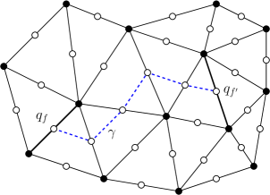
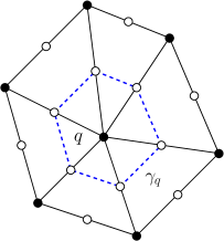
(a)                                                        (b)

Figure 2. (a) Illustration of a piecewise affine path $\gamma\in\Gamma_{f,f^{\prime}}$. (b) Illustration of the path $\gamma_{q}$ used in the proof of Lemma 5.2.

For any piecewise constant vector field $\sigma\in{\rm P}_{0}(\mathscr{T}_{\varepsilon}^{\#})^{2}$ and for any path $\gamma\in\Gamma_{f,f^{\prime}}$, $\gamma=\{x(t)\,|\,0\leq t\leq T\}$, we denote the standard path integral by

$$\int_{\gamma}\sigma\cdot\,{\rm d}x=\int_{t=0}^{T}\sigma\cdot\dot{x}(t)\,{\rm d}t.$$

For piecewise constant tensor fields $\sigma\in{\rm P}_{0}(\mathscr{T}_{\varepsilon}^{\#})^{k\times 2}$ we define the path integral as

$$\int_{\gamma}\sigma\cdot\,{\rm d}x=\int_{t=0}^{T}\sigma\dot{x}(t)\,{\rm d}t.$$

Since functions $w\in{\rm N}_{1}(\mathscr{T}_{\varepsilon}^{\#})^{k}$ have piecewise constant gradients $\nabla w$, and since they are continuous in edge midpoints, it is easy to see that

$$\int_{\gamma}\nabla w\cdot\,{\rm d}x=w(q_{f^{\prime}})-w(q_{f})\qquad\forall\gamma\in\Gamma_{f,f^{\prime}}.$$ (41)

Discrete divergence-free tensor fields

The following lemma characterizes discrete divergence-free tensor fields.

Lemma 9. A tensor field $\sigma\in{\rm P}_{0}^{\#}(\mathscr{T}_{\varepsilon})^{k\times 2}$ satisfies

$$\int_{\Omega}\sigma:\nabla u\,{\rm d}x=0\qquad\forall u\in{\rm P}_{1}^{\#}(\mathscr{T}_{\varepsilon})^{k}$$

if and only if there exist a constant $\sigma_{0}\in\mathbb{R}^{k\times 2}$ and a function $w\in{\rm N}_{1}^{\#}(\mathscr{T}_{\varepsilon})^{k}$ such that

$$\sigma=\sigma_{0}+\nabla w{\sf J},\qquad\text{where}\quad{\sf J}=\left[\begin{matrix}0&-1\\ 1&0\end{matrix}\right]\in{\rm SO}(2).$$

Sketch of the proof.

The reverse direction, that any tensor field of the form $\sigma=\sigma_{0}+\nabla w{\sf J}$ has zero discrete divergence, can be checked using a straightforward calculation, using (41).

Step 0. Outline: To simplify the notation, we define $\alpha=\sigma{\sf J}^{T}$ and, without loss of generality, we assume that $k=1$. Initially, we treat $\alpha$ as a piecewise constant tensor field on all of $\mathbb{R}^{2}$, ignoring periodicity. We construct $w\in{\rm N}_{1}(\mathscr{T}_{\varepsilon}^{\#})$ by explicitly specifying $w(q_{f})$ for all edges $f\in\mathscr{F}_{\varepsilon}^{\#}$. We will then show in the last step of the proof that $w$ can be written as the sum of an affine function and a periodic function.

Step 1. Construction of $w$: Fix a starting edge $\hat{f}\in\mathscr{F}_{\varepsilon}$ and define $w(q_{\hat{f}})=0$. For any edge $f\in\mathscr{F}_{\varepsilon}^{\#}$ let $\gamma\in\Gamma_{\hat{f},f}$ and define $w(q_{f})$ via the path integral

$$w(q_{f}):=\int_{\gamma}\alpha\cdot\,{\rm d}x.$$

We need to show that this definition is independent of the path.

Let $q$ be a vertex of the triangulation $\mathscr{T}_{\varepsilon}^{\#}$ and let $\varphi_{q}$ be the corresponding nodal basis function with support $\omega_{q}$; then a fairly straightforward calculation (see, e.g., [48] for the details) shows that

$$0=\int_{\omega_{q}}\sigma\cdot\nabla\varphi_{q}\,{\rm d}x=\frac{1}{2}\sum_{\begin{subarray}{c}f\in\mathscr{F}_{\varepsilon}^{\#}\\ f\subset{\rm int}(\omega_{q})\end{subarray}}\Big{(}\big{(}\sigma\cdot\nu_{f}\big{)}^{+}+\big{(}\sigma\cdot\nu_{f}\big{)}^{-}\Big{)}=\int_{\gamma_{q}}\alpha\cdot\,{\rm d}x,$$

where $\nu_{f}^{\pm}$ are the two unit normals to $f$, and $\gamma_{q}$ is the piecewise affine path through edge midpoints circling $q$; cf. Figure 2(b). Note that the rotation ${\sf J}$ in the definition of $\alpha$ comes from the fact that tangent vectors are rotated normal vectors.

Since all closed piecewise affine paths can be written as a sum over paths $\gamma_{q}$, this implies that $\int_{\gamma}\alpha\cdot\,{\rm d}x=0$ for all closed piecewise affine paths $\gamma$, and in particular that the definition of $w(q_{f})$ is independent of the choice of path, that is, $w$ is well-defined.

Step 2. $\nabla w=\alpha$: From the definition of $w(q_{f})$, $f\in\mathscr{F}_{\varepsilon}^{\#}$, it follows that, for $f,f^{\prime}\subset T\in\mathscr{T}_{\varepsilon}^{\#}$,

$$\nabla w(T)\cdot(q_{f}-q_{f^{\prime}})=w(q_{f})-w(q_{f^{\prime}})=\alpha(T)\cdot(q_{f}-q_{f^{\prime}}),$$

which immediately implies that $\nabla w(T)=\alpha(T)$.

Step 3. Periodicity: We are only left to show that $w(x)=a\cdot x+w_{1}(x)$ for some $a\in\mathbb{R}^{2}$, $a=(a_{1},a_{2})$, and $w_{1}\in{\rm N}_{1}^{\#}(\mathscr{T}_{\varepsilon})$. Let $a_{j}=w(q_{\hat{f}}+2e_{j})$, $j=1,2$, and define $w_{1}(x)=w(x)-a\cdot x$. Fix $j\in\{1,2\}$, let $f\in\mathscr{F}_{\varepsilon}^{\#}$ and let $\gamma$ be a path from $q_{\hat{f}}$ to $q_{f}$. Since $\alpha$ is $2\mathbb{Z}^{2}$-periodic, and since $w_{1}(q_{\hat{f}}+2e_{j})=w_{1}(q_{\hat{f}})=0$, we have

$$w_{1}(q_{f}+2e_{j})=\int_{\gamma+2e_{j}}\alpha\cdot\,{\rm d}x=\int_{\gamma}\alpha\cdot\,{\rm d}x=w_{1}(q_{f}).$$

This shows that $w_{1}$ is periodic and thus concludes the proof. ∎

6. A General Consistency Result in 2D

We are now finally in a position to make precise the statement that patch test consistent a/c methods are first-order consistent. Motivated by the example of the QNL consistency result (ignoring, as discussed in §4.3, the second-order consistency of the Cauchy–Born approximation), we would like to prove a result of the form

$$\big{\|}\delta\mathscr{E}_{\rm ac}(y)-\delta\mathscr{E}_{\rm a}(y)\big{\|}_{{\rm W}^{-1,p}_{\varepsilon}}\leq C\varepsilon\big{\|}\nabla^{2}y\big{\|}_{{\rm L}^{p}(\Omega_{\rm c}\cup\Omega_{\rm i})}.$$

As explained in §3.2 we will use the oscillation operator (24) to replace the undefined second derivative.

For each element $T\in\mathscr{T}_{\varepsilon}^{\#}$, let $\omega_{T}^{\rm a}$ be the interaction neighbourhood of $T$ in the atomistic model,

$$\omega_{T}^{\rm a}:=\big{\{}x+t_{1}r_{1}+t_{2}r_{2}\,\big{|}\,x\in T,t_{i}\in[0,1],r_{i}\in\mathscr{R}\big{\}},$$ (42)

and $\omega_{T}$ its union with the set $\omega_{T}^{\rm c}$, restricted to the continuum and interface regions,

$$\omega_{T}:=\bigg{(}\omega_{T}^{\rm a}\cup\bigcup_{\begin{subarray}{c}T^{\prime}\in\mathscr{T}_{\varepsilon}^{\#}\\ T\cap T^{\prime}\neq\emptyset\end{subarray}}T^{\prime}\bigg{)}\setminus\Omega_{\rm a}^{\#}.$$ (43)

Note that assumption (16) implies that $\omega_{T}^{\rm a}\cup\omega_{T}^{\rm c}\subset\omega_{T}$ for all $T\in\mathscr{T}_{\varepsilon}^{\rm c}$.

Theorem 10 (First-order Consistency of Patch Test Consistent a/c Methods).  Suppose that $\mathscr{E}_{\rm ac}$ is patch test consistent (§2.3) and globally energy consistent (§2.3), that the locality condition (21) and the scaling condition (22) hold, that ${\rm int}(\Omega_{\rm a})$ is connected, that $\mathscr{T}_{h}^{\rm a}\cup\mathscr{T}^{\rm i}_{h}\subset\mathscr{T}_{\varepsilon}$, and that (16) holds. Then, for any $y\in\mathscr{Y},$ we have

$$\big{\|}\delta\mathscr{E}_{\rm ac}(y)-\delta\mathscr{E}_{\rm a}(y)\big{\|}_{{\rm W}^{-1,p}_{\varepsilon}}\leq\varepsilon\bigg{\{}\sum_{T\in\mathscr{T}_{\varepsilon}^{\rm c}\cup\mathscr{T}_{\varepsilon}^{\rm i}}|T|\Big{[}M_{T}\,{\rm osc}(\nabla y;\omega_{T})\Big{]}^{p}\bigg{\}}^{1/p},$$ (44)

where the oscillation measure ${\rm osc}$ is defined in (24), the interaction neighbourhood $\omega_{T}$ is defined in (43), and the prefactors $M_{T}$ are defined as follows:

$$M_{T}=\left\{\begin{array}[]{rl}0,&T\in\mathscr{T}_{\varepsilon}^{\rm a},\\ \big{(}M^{\rm i}+M^{\rm a}\big{)}\big{(}1+7\,{\rm width}(\Omega_{\rm i})\big{)},&T\in\mathscr{T}_{\varepsilon}^{\rm i},\\ M^{\rm a}+7\big{(}M^{\rm i}+M^{\rm a}\big{)}{\rm width}(\Omega_{\rm i}),&T\in\mathscr{T}_{\varepsilon}^{\rm c}.\end{array}\right.$$ (45)

In (45), the constants $M^{\rm a}$ and $M^{\rm i}$ are defined in (6) and (23), and the “interface width” ${\rm width}(\Omega_{\rm i})$ is given by

$${\rm width}(\Omega_{\rm i}):=\max_{\begin{subarray}{c}f\in\mathscr{F}_{\varepsilon}\\ f\subset\Omega_{\rm i}^{\#}\end{subarray}}\min_{\begin{subarray}{c}f^{\prime}\in\mathscr{F}_{\varepsilon}^{\#}\\ f^{\prime}\subset\Omega_{\rm a}^{\#}\end{subarray}}\min_{\gamma\in\Gamma_{f,f^{\prime}}}\,\frac{{\rm length}(\gamma)}{\varepsilon}.$$ (46)

Outline of the proof.

We will construct “stress functions” $\Sigma_{\rm a}(y),\Sigma_{\rm ac}(y)\in{\rm P}_{0}(\mathscr{T}_{\varepsilon})^{2\times 2}$ such that

$$\big{\langle}\delta\mathscr{E}_{\rm a}(y),u\big{\rangle}=\int_{\Omega}\Sigma_{\rm a}(y):\nabla u\,{\rm d}x,\quad\text{and}\quad\big{\langle}\delta\mathscr{E}_{\rm ac}(y);u\big{\rangle}=\int_{\Omega}\Sigma_{\rm ac}(y):\nabla u\,{\rm d}x\qquad\forall u\in\mathscr{U}.$$

If we could prove an estimate of the form

$$\big{|}\Sigma_{\rm a}(y;T)-\Sigma_{\rm ac}(y;T)\big{|}\lesssim\varepsilon\,{\rm osc}(\nabla y;\omega_{T}),$$

then the result would follow immediately. It turns out that this is not possible.

Instead, we will use the fact that $\mathscr{E}_{\rm ac}$ is globally energy consistent and patch test consistent to construct a correction (cf. Corollary 6.2, Lemma 6.2, and §6.2)

$$\widehat{\Sigma}_{\rm ac}(y)=\Sigma_{\rm ac}(y)-\nabla\hat{\psi}(y){\sf J},$$

which still represents the first variation $\delta\mathscr{E}_{\rm ac}$ (cf. Lemma 5.2), and which has the property that

$$\Sigma_{\rm a}(y_{\sf F};T)=\widehat{\Sigma}_{\rm ac}(y_{\sf F};T)=\partial W({\sf F})\qquad\forall\,T\in\mathscr{T}_{\varepsilon}^{\rm c}\cup\mathscr{T}_{\varepsilon}^{\rm i},\quad{\sf F}\in\mathbb{R}^{2\times 2}.$$

In addition, we show that $\widehat{\Sigma}_{\rm ac}(y;T)=\Sigma_{\rm a}(y;T)$ for all $T\in\mathscr{T}_{\varepsilon}^{\rm a}$.

Lipschitz estimates for $\Sigma_{\rm a}$ and $\widehat{\Sigma}_{\rm ac}$, and careful modifications of the argument in the interface region, yield the following result (cf. Lemma 6.3):

$$\big{|}\widehat{\Sigma}_{\rm ac}(y;T)-\Sigma_{\rm a}(y;T)\big{|}\leq~{} \big{|}\widehat{\Sigma}_{\rm ac}(y;T)-\partial W(\nabla y(T))\big{|}+\big{|}\Sigma_{\rm a}(y;T)-\partial W(\nabla y(T))\big{|}$$

$$\leq~{} \varepsilon M_{T}{\rm osc}(\nabla y;\omega_{T})\qquad\forall T\in\mathscr{T}_{\varepsilon},$$

and, in particular,

$$\big{\langle}\delta\mathscr{E}_{\rm ac}(y)-\delta\mathscr{E}_{\rm a}(y);u\big{\rangle}=~{} \sum_{T\in\mathscr{T}_{\varepsilon}}|T|\Big{[}\widehat{\Sigma}_{\rm ac}(y;T)-\Sigma_{\rm a}(y;T)\Big{]}:\nabla u(T)$$

$$\leq~{} \varepsilon\bigg{\{}\sum_{T\in\mathscr{T}_{\varepsilon}^{\rm c}\cup\mathscr{T}_{\varepsilon}^{\rm i}}|T|\Big{[}M_{T}\,{\rm osc}(\nabla y;\omega_{T})\Big{]}^{p}\bigg{\}}^{1/p}\,\big{\|}\nabla u\|_{{\rm L}^{p^{\prime}}(\Omega)},$$

which yields the stated first order consistency estimate. ∎

Remark 8. In 1D, a similar result can be proven using a similar framework but with significantly reduced technicalities. Note, in particular, that the 1D analogue of Lemma 5.2 is

$$\int_{\Omega}\sigma\cdot\nabla u\,{\rm d}x=0\quad\forall\,u\in\mathscr{U}\qquad\text{if and only if}\qquad\sigma\text{ is constant}.$$

Hence, the corrector function $\psi({\sf F},\cdot)$ defined in §6.2 is always identically equal to zero, which removes the interface width dependence from the modelling error (cf. §6.3). Hence, if $d=1$, we obtain (44) again but with modified prefactors

$$M_{T}^{\rm 1D}:=\left\{\begin{array}[]{rl}0,&T\in\mathscr{T}_{\varepsilon}^{\rm a},\\ M^{\rm i}+M^{\rm a},&T\in\mathscr{T}_{\varepsilon}^{\rm i},\\ M^{\rm a},&T\in\mathscr{T}_{\varepsilon}^{\rm c}.\end{array}\right.$$ (47)

Moreover, since $\psi\equiv 0$ in 1D, and since symmetries are more easily exploited, it is not too difficult in 1D to prove second order consistency in the continuum region. ∎

6.1. The atomistic stress function

A natural “weak” representation of $\delta\mathscr{E}_{\rm a}(y)$, $y\in\mathscr{Y}$, is given by

$$\langle\delta\mathscr{E}_{\rm a}(y),z\rangle=\varepsilon^{2}\sum_{x\in\mathscr{L}}\sum_{r\in\mathscr{R}}\partial_{r}V(D_{\!\mathscr{R}})\cdot D_{\!r}z(x),\qquad\text{for }z\in\mathscr{Y}.$$ (48)

Using bond integrals we rewrite this in a form that will be useful for our subsequent analysis. We will then use the bond density lemma whenever we need to transition between bond integrals and volume integrals. This process yields a notion of stress for atomistic models, which is related to the virial stress (see [2] for a recent reference; this connection will be discussed in detail elsewhere). A variant of this result for pair interactions in 1D was developed in [32].

Proposition 11. Let $y,z\in\mathscr{Y}$, then

$$\langle\delta\mathscr{E}_{\rm a}(y),z\rangle=\sum_{T\in\mathscr{T}_{\varepsilon}}|T|\,\Sigma_{\rm a}(y;T):\nabla z(T)=\int_{\Omega}\Sigma_{\rm a}(y):\nabla z\,{\rm d}x,$$

where the stress function $\Sigma_{\rm a}(y)\in{\rm P}_{0}^{\#}(\mathscr{T}_{\varepsilon})^{2\times 2}$ is defined as follows:

$$\Sigma_{\rm a}(y;T):=\sum_{r\in\mathscr{R}}\frac{\varepsilon^{2}}{|T|}\sum_{x\in\mathscr{L}^{\#}}\Big{[}\partial_{r}V\big{(}D_{\!\mathscr{R}}y(x)\big{)}\otimes r\Big{]}\mathchoice{{\vbox{\hbox{$\textstyle-$ }}\kern-7.83337pt}}{{\vbox{\hbox{$\scriptstyle-$ }}\kern-5.90005pt}}{{\vbox{\hbox{$\scriptscriptstyle-$ }}\kern-4.75003pt}}{{\vbox{\hbox{$\scriptscriptstyle-$ }}\kern-4.25003pt}}\!\int_{x}^{x+\varepsilon r}\chi_{T}\,{\rm db}.$$ (49)

Proof.

For the sake of brevity we will write $V_{x,r}=\partial_{r}V(D_{\!\mathscr{R}}y(x))$.

Recall that $T^{\#}=\bigcup_{\xi\in 2\mathbb{Z}^{2}}(\xi+T)$, for $T\in\mathscr{T}_{\varepsilon}$. It is easy to see that $\{\chi_{T^{\#}}\,|\,T\in\mathscr{T}_{\varepsilon}\}$ is a partition of unity for $\mathbb{R}^{2}$. Hence, using the identity

$$\mathchoice{{\vbox{\hbox{$\textstyle-$ }}\kern-7.83337pt}}{{\vbox{\hbox{$\scriptstyle-$ }}\kern-5.90005pt}}{{\vbox{\hbox{$\scriptscriptstyle-$ }}\kern-4.75003pt}}{{\vbox{\hbox{$\scriptscriptstyle-$ }}\kern-4.25003pt}}\!\int_{x}^{x+\varepsilon r}\nabla_{\!\!r}z\,{\rm db}=D_{\!r}z(x),$$ (50)

we can rewrite (48) as

$$\big{\langle}\delta\mathscr{E}_{\rm a}(y),z\big{\rangle}=\varepsilon^{2}\sum_{x\in\mathscr{L}}\sum_{r\in\mathscr{R}}V_{x,r}\cdot\mathchoice{{\vbox{\hbox{$\textstyle-$ }}\kern-7.83337pt}}{{\vbox{\hbox{$\scriptstyle-$ }}\kern-5.90005pt}}{{\vbox{\hbox{$\scriptscriptstyle-$ }}\kern-4.75003pt}}{{\vbox{\hbox{$\scriptscriptstyle-$ }}\kern-4.25003pt}}\!\int_{x}^{x+\varepsilon r}\Big{[}\sum_{T\in\mathscr{T}_{\varepsilon}}\chi_{T^{\#}}\Big{]}\nabla_{\!\!r}z\,{\rm db}.$$

Interchanging the order of summation and using the fact that $\nabla_{\!\!r}z=(\nabla z)r$ holds $\,{\rm db}$-a.e. (note that, if the bond is aligned with an element edge, then $\nabla_{\!\!r}z$ is continuous across that edge) yields

$$\langle\delta\mathscr{E}_{\rm a}(y),z\rangle=\sum_{T\in\mathscr{T}_{\varepsilon}}|T|\sum_{r\in\mathscr{R}}\frac{\varepsilon^{2}}{|T|}\sum_{x\in\mathscr{L}}V_{x,r}\cdot\mathchoice{{\vbox{\hbox{$\textstyle-$ }}\kern-7.83337pt}}{{\vbox{\hbox{$\scriptstyle-$ }}\kern-5.90005pt}}{{\vbox{\hbox{$\scriptscriptstyle-$ }}\kern-4.75003pt}}{{\vbox{\hbox{$\scriptscriptstyle-$ }}\kern-4.25003pt}}\!\int_{x}^{x+\varepsilon r}\chi_{T^{\#}}\nabla z(T^{\#})r\,{\rm db}.$$

The term $\nabla z(T^{\#})r=\nabla z(T)r$ can be taken outside the bond integral, and hence, employing the identity

$$a\cdot({\sf G}r)=(a\otimes r):{\sf G},\qquad\text{for }a,r\in\mathbb{R}^{d},{\sf G}\in\mathbb{R}^{d\times d},$$ (51)

yields

$$\langle\delta\mathscr{E}_{\rm a}(y),z\rangle=~{} \sum_{T\in\mathscr{T}_{\varepsilon}}|T|\bigg{\{}\sum_{r\in\mathscr{R}}\frac{\varepsilon^{2}}{|T|}\sum_{x\in\mathscr{L}}\big{[}V_{x,r}\otimes r\big{]}\mathchoice{{\vbox{\hbox{$\textstyle-$ }}\kern-7.83337pt}}{{\vbox{\hbox{$\scriptstyle-$ }}\kern-5.90005pt}}{{\vbox{\hbox{$\scriptscriptstyle-$ }}\kern-4.75003pt}}{{\vbox{\hbox{$\scriptscriptstyle-$ }}\kern-4.25003pt}}\!\int_{x}^{x+\varepsilon r}\chi_{T^{\#}}\,{\rm db}\bigg{\}}:\nabla z(T)$$

$$=:~{} \sum_{T\in\mathscr{T}_{\varepsilon}}|T|\,\Sigma_{\rm a}(y;T):\nabla z(T).$$

Finally, we use the fact that $D_{\!\mathscr{R}}y$ is $2\mathbb{Z}^{2}$-periodic to deduce that

$$\Sigma_{\rm a}(y;T)=~{} \sum_{r\in\mathscr{R}}\frac{\varepsilon^{2}}{|T|}\sum_{x\in\mathscr{L}}\big{[}V_{x,r}\otimes r\big{]}\mathchoice{{\vbox{\hbox{$\textstyle-$ }}\kern-7.83337pt}}{{\vbox{\hbox{$\scriptstyle-$ }}\kern-5.90005pt}}{{\vbox{\hbox{$\scriptscriptstyle-$ }}\kern-4.75003pt}}{{\vbox{\hbox{$\scriptscriptstyle-$ }}\kern-4.25003pt}}\!\int_{x}^{x+\varepsilon r}\chi_{T^{\#}}\,{\rm db}$$

$$=~{} \sum_{r\in\mathscr{R}}\frac{\varepsilon^{2}}{|T|}\sum_{x\in\mathscr{L}}\big{[}V_{x,r}\otimes r\big{]}\sum_{\xi\in 2\mathbb{Z}^{2}}\mathchoice{{\vbox{\hbox{$\textstyle-$ }}\kern-7.83337pt}}{{\vbox{\hbox{$\scriptstyle-$ }}\kern-5.90005pt}}{{\vbox{\hbox{$\scriptscriptstyle-$ }}\kern-4.75003pt}}{{\vbox{\hbox{$\scriptscriptstyle-$ }}\kern-4.25003pt}}\!\int_{x}^{x+\varepsilon r}\chi_{\xi+T}\,{\rm db}$$

$$=~{} \sum_{r\in\mathscr{R}}\frac{\varepsilon^{2}}{|T|}\sum_{x\in\mathscr{L}^{\#}}\big{[}V_{x,r}\otimes r\big{]}\mathchoice{{\vbox{\hbox{$\textstyle-$ }}\kern-7.83337pt}}{{\vbox{\hbox{$\scriptstyle-$ }}\kern-5.90005pt}}{{\vbox{\hbox{$\scriptscriptstyle-$ }}\kern-4.75003pt}}{{\vbox{\hbox{$\scriptscriptstyle-$ }}\kern-4.25003pt}}\!\int_{x}^{x+\varepsilon r}\chi_{T}\,{\rm db}.\qed$$

The terminology “stress function” for $\Sigma_{\rm a}$ is motivated by the fact that $\Sigma_{\rm a}(y)$ takes precisely the same role as the first Piola–Kirchhoff stress tensor in the continuum theory of elasticity.

In the next lemma we prove two useful properties of the atomistic stress function $\Sigma_{\rm a}$. We show that $\Sigma_{\rm a}=\partial W$ under locally homogeneous deformations and give a quantitative estimate for the discrepancy between $\Sigma_{\rm a}$ and $\partial W$.

Lemma 12. The stress function $\Sigma_{\rm a}$ defined in (49) satisfies

$$\Sigma_{\rm a}(y_{\sf F};T)=\partial W({\sf F})\qquad\forall{\sf F}\in\mathbb{R}^{2\times 2},\quad T\in\mathscr{T}_{\varepsilon}.$$

Moreover, we have the estimate

$$\big{|}\Sigma_{\rm a}(y;T)-\partial W\big{(}\nabla y(T)\big{)}\big{|}\leq\varepsilon M^{\rm a}{\rm osc}(\nabla y;\omega_{T}^{\rm a})\qquad\forall y\in\mathscr{Y},\quad T\in\mathscr{T}_{\varepsilon},$$ (52)

where $M^{\rm a}$ is defined in (6) and $\omega_{T}^{\rm a}$ is defined in (42).

Proof.

Part 1: Since $[\partial_{r}V({\sf F}\mathscr{R})\otimes r]$ is independent of $x$, we can apply the bond density lemma to the sum in curly brackets, to deduce that

$$\Sigma_{\rm a}(y_{\sf F};T)=\sum_{r\in\mathscr{R}}\Big{[}\partial_{r}V\big{(}{\sf F}\mathscr{R}\big{)}\otimes r\Big{]}\bigg{\{}\frac{\varepsilon^{2}}{|T|}\sum_{x\in\mathscr{L}^{\#}}\mathchoice{{\vbox{\hbox{$\textstyle-$ }}\kern-7.83337pt}}{{\vbox{\hbox{$\scriptstyle-$ }}\kern-5.90005pt}}{{\vbox{\hbox{$\scriptscriptstyle-$ }}\kern-4.75003pt}}{{\vbox{\hbox{$\scriptscriptstyle-$ }}\kern-4.25003pt}}\!\int_{x}^{x+\varepsilon r}\chi_{T}\,{\rm db}\bigg{\}}=\sum_{r\in\mathscr{R}}\Big{[}\partial_{r}V\big{(}{\sf F}\mathscr{R}\big{)}\otimes r\Big{]}.$$

Recalling that $W({\sf F})=V({\sf F}\mathscr{R})$, it can be easily checked that the sum on the right-hand side of the second equality equals $\partial W({\sf F})$.

Part 2: Let ${\sf F}=\nabla y(T)$, $V_{x,r}=\partial_{r}V(D_{\!\mathscr{R}}y(x))$, and $V_{{\sf F},r}=\partial_{r}V({\sf F}\mathscr{R})$. From part 1 we obtain that

$$\big{|}\Sigma_{\rm a}(y;T)-\partial W({\sf F})\big{|}=~{} \bigg{|}\sum_{r\in\mathscr{R}}\frac{\varepsilon^{2}}{|T|}\sum_{x\in\mathscr{L}^{\#}}\Big{[}\big{(}V_{x,r}-V_{{\sf F},r}\big{)}\otimes r\Big{]}\mathchoice{{\vbox{\hbox{$\textstyle-$ }}\kern-7.83337pt}}{{\vbox{\hbox{$\scriptstyle-$ }}\kern-5.90005pt}}{{\vbox{\hbox{$\scriptscriptstyle-$ }}\kern-4.75003pt}}{{\vbox{\hbox{$\scriptscriptstyle-$ }}\kern-4.25003pt}}\!\int_{x}^{x+\varepsilon r}\chi_{T}\,{\rm db}\bigg{|}$$

$$\leq~{} \sum_{r\in\mathscr{R}}|r|\frac{\varepsilon^{2}}{|T|}\sum_{x\in\mathscr{L}^{\#}}\Big{|}V_{x,r}-V_{{\sf F},r}\Big{|}\mathchoice{{\vbox{\hbox{$\textstyle-$ }}\kern-7.83337pt}}{{\vbox{\hbox{$\scriptstyle-$ }}\kern-5.90005pt}}{{\vbox{\hbox{$\scriptscriptstyle-$ }}\kern-4.75003pt}}{{\vbox{\hbox{$\scriptscriptstyle-$ }}\kern-4.25003pt}}\!\int_{x}^{x+\varepsilon r}\chi_{T}\,{\rm db}.$$ (53)

We use the Lipschitz property 5 to estimate

$$\big{|}V_{x,r}-V_{{\sf F},r}\big{|}\leq~{} \sum_{s\in\mathscr{R}}M_{r,s}^{\rm a}\big{|}D_{\!s}y(x)-{\sf F}s\big{|}$$

$$=~{} \sum_{s\in\mathscr{R}}M_{r,s}^{\rm a}\bigg{|}\mathchoice{{\vbox{\hbox{$\textstyle-$ }}\kern-7.83337pt}}{{\vbox{\hbox{$\scriptstyle-$ }}\kern-5.90005pt}}{{\vbox{\hbox{$\scriptscriptstyle-$ }}\kern-4.75003pt}}{{\vbox{\hbox{$\scriptscriptstyle-$ }}\kern-4.25003pt}}\!\int_{x}^{x+\varepsilon s}\Big{(}\nabla_{\!\!s}y-{\sf F}s\Big{)}\,{\rm db}\bigg{|}$$

$$\leq~{} \sum_{s\in\mathscr{R}}M_{r,s}^{\rm a}|s|\max_{x^{\prime}\in(x,x+\varepsilon s)}\big{|}\nabla y(x^{\prime})-{\sf F}\big{|}.$$ (54)

Since $(x,x+\varepsilon s)\subset\omega_{T}^{\rm a}$, and recalling that ${\sf F}=\nabla y(T)$, we can further estimate

$$\max_{x^{\prime}\in(x,x+\varepsilon s)}\big{|}\nabla y(x^{\prime})-{\sf F}\big{|}\leq\varepsilon{\rm osc}(\nabla y;\omega_{T}^{\rm a}).$$ (55)

We combine (55) with (54) and insert the resulting estimate into (53) to arrive at

$$\big{|}\Sigma_{\rm a}(y;T)-\partial W({\sf F})\big{|}\leq\varepsilon{\rm osc}(\nabla y;\omega_{T}^{\rm a})\sum_{r\in\mathscr{R}}\sum_{s\in\mathscr{R}}|r||s|M_{r,s}^{\rm a}\frac{\varepsilon^{2}}{|T|}\sum_{x\in\mathscr{L}^{\#}}\mathchoice{{\vbox{\hbox{$\textstyle-$ }}\kern-7.83337pt}}{{\vbox{\hbox{$\scriptstyle-$ }}\kern-5.90005pt}}{{\vbox{\hbox{$\scriptscriptstyle-$ }}\kern-4.75003pt}}{{\vbox{\hbox{$\scriptscriptstyle-$ }}\kern-4.25003pt}}\!\int_{x}^{x+\varepsilon r}\chi_{T}\,{\rm db}.$$

An application of the bond density lemma, and referring to the definition of $M^{\rm a}$ in (6), yields the stated result. ∎

6.2. The a/c stress function

We wish to derive a similar representation of $\delta\mathscr{E}_{\rm ac}$ in terms of a stress function $\Sigma_{\rm ac}$, as we did in §6.1 for $\delta\mathscr{E}_{\rm a}$. A straightforward calculation along the same lines as the proof of Proposition 6.1, recalling first the definition of the partial derivative $\partial_{b}E_{\rm i}$ from §2.3, yields the following result.

Proposition 13. Suppose that (16) holds, then, for all $y,z\in\mathscr{Y}$,

$$\big{\langle}\delta\mathscr{E}_{\rm ac}(y),z\big{\rangle}=\sum_{T\in\mathscr{T}_{\varepsilon}}|T|\,\Sigma_{\rm ac}(y;T):\nabla z(T)=\int_{\Omega}\Sigma_{\rm ac}(y):\nabla z\,{\rm d}x,$$

where

$$\Sigma_{\rm ac}(y;T):=\left\{\begin{array}[]{rl}\Sigma_{\rm a}(y;T),&T\in\mathscr{T}_{\varepsilon}^{\rm a},\\[5.69054pt] \partial W(\nabla y(T)),&T\in\mathscr{T}_{\varepsilon}^{\rm c},\\[5.69054pt] \sum_{r\in\mathscr{R}}\frac{\varepsilon^{2}}{|T|}\sum_{x\in\mathscr{L}_{\rm a}^{\#}}\big{[}\partial_{r}V\big{(}D_{\!\mathscr{R}}y(x)\big{)}\otimes r\big{]}\mathchoice{{\vbox{\hbox{$\textstyle-$ }}\kern-7.83337pt}}{{\vbox{\hbox{$\scriptstyle-$ }}\kern-5.90005pt}}{{\vbox{\hbox{$\scriptscriptstyle-$ }}\kern-4.75003pt}}{{\vbox{\hbox{$\scriptscriptstyle-$ }}\kern-4.25003pt}}\!\int_{x}^{x+\varepsilon r}\chi_{T}\,{\rm db}&\\ +\frac{\varepsilon^{2}}{|T|}\sum_{(x,x+\varepsilon r)\in\mathscr{B}_{\rm i}^{\#}}\big{[}\partial_{(x,x+\varepsilon r)}E_{\rm i}(y)\otimes r\big{]}\mathchoice{{\vbox{\hbox{$\textstyle-$ }}\kern-7.83337pt}}{{\vbox{\hbox{$\scriptstyle-$ }}\kern-5.90005pt}}{{\vbox{\hbox{$\scriptscriptstyle-$ }}\kern-4.75003pt}}{{\vbox{\hbox{$\scriptscriptstyle-$ }}\kern-4.25003pt}}\!\int_{x}^{x+\varepsilon r}\chi_{T}^{\rm i}\,{\rm db},&T\in\mathscr{T}_{\varepsilon}^{\rm i}.\end{array}\right.$$

where $\chi_{T}^{\rm i}$ is a modified characteristic function:

$$\chi_{T}^{\rm i}(x)=\left\{\begin{array}[]{rl}1,&x\in\partial\Omega_{\rm i}^{\#},\\ \chi_{T}(x),&\text{otherwise}.\end{array}\right.$$

Proof.

Employing again the notation $V_{x,r}=\partial_{r}V(D_{\!\mathscr{R}}y(x))$, the functional $\delta\mathscr{E}_{\rm ac}(y)$ can be written as

$$\begin{split}\big{\langle}\delta\mathscr{E}_{\rm ac}(y),z\big{\rangle}=~{}&\int_{\Omega_{\rm c}}\partial W(\nabla y):\nabla z\,{\rm d}x+\varepsilon^{2}\sum_{x\in\mathscr{L}_{\rm a}}\sum_{r\in\mathscr{R}}V_{x,r}\cdot D_{\!r}u(x)\\ &+\varepsilon^{2}\sum_{(x,x+\varepsilon r)\in\mathscr{B}_{\rm i}}\partial_{(x,x+\varepsilon r)}E_{\rm i}(y)\cdot D_{\!r}u(x).\end{split}$$ (56)

The first term on the right-hand side of (56) gives rise to the definition of $\Sigma_{\rm ac}(y;T)$ for $T\in\mathscr{T}_{\varepsilon}^{\rm c}$. (Note that (16) guarantees that the bonds in the second group in (56) do not contribute to $\Omega_{\rm c}$.)

After the same calculation as in the proof of Proposition 6.1, the second group on the right-hand side of (56) gives the definition of $\Sigma_{\rm ac}(y;T)$ for $T\in\mathscr{T}_{\varepsilon}^{\rm a}$, as well as the first group in the definition of $\Sigma_{\rm ac}(y;T)$ for $T\in\mathscr{T}_{\varepsilon}^{\rm i}$.

The crucial modification to the previous argument is that the modified characteristic functions $\chi_{T}^{\rm i}$, $T\in\mathscr{T}_{\varepsilon}^{\rm i}$ form a partition of unity for $\Omega_{\rm i}$ (except at a finite number of points, which do not contribute to bond integrals). Therefore, performing again a similar calculation as in the proof of Proposition 6.1 to “distribute” the third group on the right-hand side of (56) between interface elements only, we obtain the second group in the definition of $\Sigma_{\rm ac}(y;T)$ for $T\in\mathscr{T}_{\varepsilon}^{\rm i}$.

Note that if we hadn’t made the modification to the characteristic function, then $\Sigma_{\rm ac}(y;T)$, $T\in\mathscr{T}_{\varepsilon}^{\rm a}\cup\mathscr{T}_{\varepsilon}^{\rm c}$ would contain contributions from $E_{\rm i}$. ∎

Since any discrete divergence-free tensor field may be added to $\Sigma_{\rm ac}$ and still yield a valid representation of $\delta\mathscr{E}_{\rm ac}$, it is not surprising that, in general, $\Sigma_{\rm ac}$ does not have the necessary property that $\Sigma_{\rm ac}(y_{\sf F};T)=\partial W({\sf F})$ for all ${\sf F}\in\mathbb{R}^{2\times 2}$. This can already be observed in the nearest-neighbour, flat interface constructions in [44]. Hence, we need to construct an alternative stress function $\widehat{\Sigma}_{\rm ac}$ representing $\delta\mathscr{E}_{\rm ac}$ that does have the desired properties. This construction will be undertaken in the remainder of this section, using the representation of discrete divergence-free vector fields as gradients of Crouzeix–Raviart functions discussed in §5.2.

Consequences of global energy consistency

Recall from (13) that a functional $\mathscr{E}\in{\rm C}^{1}(\mathscr{Y})$ is called globally energy consistent if $\mathscr{E}(y_{\sf F})=\mathscr{E}_{\rm a}(y_{\sf F})$ for all matrices ${\sf F}\in\mathbb{R}^{2\times 2}$. The following lemma establishes a simple but crucial consequence of this property.

Lemma 14. Suppose that $\mathscr{E}\in{\rm C}^{1}(\mathscr{Y})$ is globally energy consistent, then

$$\langle\delta\mathscr{E}(y_{\sf F}),y_{\sf G}\rangle=|\Omega|\,\partial W({\sf F}):{\sf G}\qquad\forall\,{\sf F},{\sf G}\in\mathbb{R}^{2\times 2}.$$

Proof.

From the assumption of global energy consistency, and (12), we obtain that

$$\mathscr{E}(y_{\sf F})=\mathscr{E}_{\rm a}(y_{\sf F})=|\Omega|W({\sf F})\qquad\forall{\sf F}\in\mathbb{R}^{2\times 2}.$$

Since $y_{\sf F}+ty_{\sf G}=y_{{\sf F}+t{\sf G}}$ this implies that

$$\big{\langle}\delta\mathscr{E}(y_{\sf F}),y_{\sf G}\big{\rangle}=|\Omega|\lim_{t\to 0}\frac{W({\sf F}+t{\sf G})-W({\sf F})}{t}=|\Omega|\partial W({\sf F}):{\sf G}.\qed$$

If we apply the foregoing lemma to an a/c functional $\mathscr{E}_{\rm ac}$ we obtain the following corollary.

Corollary 15. Suppose that $\mathscr{E}_{\rm ac}$ is globally energy consistent, then

$$\mathchoice{{\vbox{\hbox{$\textstyle-$ }}\kern-7.83337pt}}{{\vbox{\hbox{$\scriptstyle-$ }}\kern-5.90005pt}}{{\vbox{\hbox{$\scriptscriptstyle-$ }}\kern-4.75003pt}}{{\vbox{\hbox{$\scriptscriptstyle-$ }}\kern-4.25003pt}}\!\int_{\Omega}\Sigma_{\rm ac}(y_{\sf F})\,{\rm d}x=\partial W({\sf F})\qquad\forall{\sf F}\in\mathbb{R}^{2\times 2}.$$

Proof.

This result follows simply from Lemma 6.2 and the fact that, for all ${\sf G}\in\mathbb{R}^{2\times 2}$,

$$\big{\langle}\delta\mathscr{E}_{\rm ac}(y_{\sf F}),y_{\sf G}\big{\rangle}=\int_{\Omega}\Sigma_{\rm ac}(y_{\sf F}):{\sf G}\,{\rm d}x=\bigg{(}\int_{\Omega}\Sigma_{\rm ac}(y_{\sf F})\,{\rm d}x\bigg{)}:{\sf G}.\qed$$

Consequences of patch test consistency

The examples given in [44] show that patch test consistency does not necessarily imply that $\Sigma_{\rm ac}(y_{\sf F};T)=\partial W({\sf F})$. In the current paragraph we characterise the discrepancy between $\Sigma_{\rm ac}(y_{\sf F};T)$ and $\partial W({\sf F})$.

First, we show that the test functions $u_{h}\in\mathscr{U}_{h}$ in the patch test (14) may be replaced by arbitrary displacements $u\in\mathscr{U}$.

Lemma 16. Suppose that $\mathscr{E}_{\rm ac}$ is patch test consistent and that $\mathscr{T}_{h}^{\rm a}\cup\mathscr{T}^{\rm i}_{h}\subset\mathscr{T}_{\varepsilon}$; then we also have

$$\big{\langle}\delta\mathscr{E}_{\rm ac}(y_{\sf F}),u\big{\rangle}=0\qquad\forall\,u\in\mathscr{U},\quad{\sf F}\in\mathbb{R}^{2\times 2}.$$ (57)

Proof.

Fix $u\in\mathscr{U}$; then, using the assumption that $\mathscr{T}_{h}^{\rm a}\cup\mathscr{T}^{\rm i}_{h}\subset\mathscr{T}_{\varepsilon}$, we have

$$\int_{\Omega_{\rm c}}\nabla u\,{\rm d}x=\int_{(\partial\Omega_{\rm c}^{\#})\cap\Omega}u\otimes\nu\,{\rm d}s=\int_{(\partial\Omega_{\rm c}^{\#})\cap\Omega}I_{h}u\otimes\nu\,{\rm d}s=\int_{\Omega_{\rm c}}\nabla I_{h}u\,{\rm d}x.$$

Since $\Sigma_{\rm ac}(y_{\sf F})=\partial W({\sf F})$ is constant in $\Omega_{\rm c}$, and since $I_{h}u=u$ in $\Omega_{\rm i}\cup\Omega_{\rm a}$, we can therefore deduce that

$$\big{\langle}\delta\mathscr{E}_{\rm ac}(y_{\sf F}),u\big{\rangle}=\int_{\Omega}\Sigma_{\rm ac}(y_{\sf F}):\nabla u\,{\rm d}x=\int_{\Omega}\Sigma_{\rm ac}(y_{\sf F}):\nabla I_{h}u\,{\rm d}x=\big{\langle}\delta\mathscr{E}_{\rm ac}(y_{\sf F}),I_{h}u\big{\rangle}=0.$$

The penultimate equality requires some justification, but follows quite easily from the particular form of $\mathscr{E}_{\rm ac}$ assumed in (18) and the assumption that $\mathscr{T}_{h}^{\rm a}\cup\mathscr{T}^{\rm i}_{h}\subset\mathscr{T}_{\varepsilon}$. ∎

Lemma 17. Suppose that $\mathscr{E}_{\rm ac}$ is patch test consistent and globally energy consistent and that $\mathscr{T}^{\rm i}_{h}\cup\mathscr{T}_{h}^{\rm a}\subset\mathscr{T}_{\varepsilon}$; then, for each ${\sf F}\in\mathbb{R}^{2\times 2}$, there exists a function $\psi({\sf F};\cdot)\in{\rm N}_{1}^{\#}(\mathscr{T}_{\varepsilon})^{2}$ such that

$$\Sigma_{\rm ac}(y_{\sf F};T)=\partial W({\sf F})+\nabla\psi({\sf F};T){\sf J}\qquad\forall\,T\in\mathscr{T}_{\varepsilon},$$

where ${\sf J}$ is a rotation matrix defined in Lemma 5.2. Moreover, if ${\rm int}(\Omega_{\rm a})$ is connected, then we may choose $\psi({\sf F})=0$ in $\Omega_{\rm a}$.

Proof.

If $\mathscr{E}_{\rm ac}$ is patch test consistent then, according to Lemma 6.2,

$$\int_{\Omega}\Sigma_{\rm ac}(y_{\sf F}):\nabla u\,{\rm d}x=\langle\delta\mathscr{E}_{\rm ac}(y_{\sf F}),u\rangle=0\qquad\forall u\in\mathscr{U}.$$

Hence, according to Lemma 5.2, there exists a constant $\Sigma_{0}\in\mathbb{R}^{2\times 2}$, a vector-valued Crouzeix–Raviart function $\psi=\psi({\sf F};\cdot)\in{\rm N}_{1}^{\#}(\mathscr{T}_{\varepsilon})^{2}$, and a rotation matrix ${\sf J}$, such that

$$\Sigma_{\rm ac}(y_{\sf F};T)=\Sigma_{0}+\nabla\psi(T){\sf J}\qquad\forall T\in\mathscr{T}_{\varepsilon}.$$

Using global energy consistency of $\mathscr{E}_{\rm ac}$ and Corollary 6.2 we obtain that

$$\partial W({\sf F})=\mathchoice{{\vbox{\hbox{$\textstyle-$ }}\kern-7.83337pt}}{{\vbox{\hbox{$\scriptstyle-$ }}\kern-5.90005pt}}{{\vbox{\hbox{$\scriptscriptstyle-$ }}\kern-4.75003pt}}{{\vbox{\hbox{$\scriptscriptstyle-$ }}\kern-4.25003pt}}\!\int_{\Omega}\Sigma_{\rm ac}(y_{\sf F})\,{\rm d}x=\Sigma_{0}+\mathchoice{{\vbox{\hbox{$\textstyle-$ }}\kern-7.83337pt}}{{\vbox{\hbox{$\scriptstyle-$ }}\kern-5.90005pt}}{{\vbox{\hbox{$\scriptscriptstyle-$ }}\kern-4.75003pt}}{{\vbox{\hbox{$\scriptscriptstyle-$ }}\kern-4.25003pt}}\!\int_{\Omega}\nabla\psi{\sf J}\,{\rm d}x.$$

If $\int_{\Omega}\nabla\psi\,{\rm d}x=0$, then $\Sigma_{0}=\partial W({\sf F})$ and hence the result follows.

To prove this, we integrate by parts separately in each element:

$$\int_{\Omega}\nabla\psi\,{\rm d}x=~{} \sum_{T\in\mathscr{T}_{\varepsilon}}\int_{\partial T}\psi\otimes\nu\,{\rm d}s=\sum_{f\in\mathscr{F}_{\varepsilon}}\big{(}\psi^{+}\otimes\nu^{+}+\psi^{-}\otimes\nu^{-}\big{)}\,{\rm d}s=0,$$

where, in the last equality, we used the fact that $\int_{f}(\psi^{+}-\psi^{-})\,{\rm d}s=0$ for all edges $f$, since $\psi$ is continuous in the edge midpoints.

Finally, since $\Sigma_{\rm ac}(y_{\sf F};T)=\partial W({\sf F})$ for all $T\in\mathscr{T}_{\varepsilon}^{\rm a}$ (cf. Lemma 6.2 and Lemma 6.1), it follows that $\nabla\psi=0$ in $\Omega_{\rm a}$. Hence, if ${\rm int}(\Omega_{\rm a})$ is connected, then we can shift $\psi$ by a constant so that $\psi=0$ in $\Omega_{\rm a}$. ∎

The modified a/c stress function

We wish to construct a modified a/c stress function $\widehat{\Sigma}_{\rm ac}$ that can be used to represent $\delta\mathscr{E}_{\rm ac}$, and satisfies the crucial property that $\widehat{\Sigma}_{\rm ac}(y_{\sf F};T)=\partial W({\sf F})$ for all ${\sf F}\in\mathbb{R}^{2\times 2}$, $T\in\mathscr{T}_{\varepsilon}^{\rm i}$.

To this end, we generalize the Crouzeix–Raviart function $\psi({\sf F})$ defined in Lemma 6.2 to arbitrary deformations $y\in\mathscr{Y}$. Since we will use later on that the modified function $\hat{\psi}$ vanishes in $\Omega_{\rm a}$, we require from now on that ${\rm int}(\Omega_{\rm a})$ is connected so that we can choose $\psi({\sf F},\cdot)=0$ in $\Omega_{\rm a}$ for all ${\sf F}\in\mathbb{R}^{2\times 2}$.

For each $y\in\mathscr{Y}$ and each face $f\in\mathscr{F}_{\varepsilon}^{\#}$, $f=T_{1}\cap T_{2}$, we define the patch $\omega_{f}=(T_{1}\cup T_{2})\setminus\Omega_{\rm a}^{\#}$, and the deformation gradient averages

$${\sf F}_{f}(y):=\left\{\begin{array}[]{rl}\mathchoice{{\vbox{\hbox{$\textstyle-$ }}\kern-7.83337pt}}{{\vbox{\hbox{$\scriptstyle-$ }}\kern-5.90005pt}}{{\vbox{\hbox{$\scriptscriptstyle-$ }}\kern-4.75003pt}}{{\vbox{\hbox{$\scriptscriptstyle-$ }}\kern-4.25003pt}}\!\int_{\omega_{f}}\nabla y\,{\rm d}x,&\text{if }|\omega_{f}|>0\\ 0,&\text{otherwise.}\end{array}\right.$$

Note that $\omega_{f}$ was defined in such a way that $\omega_{f}\subset\omega_{T_{1}}\cap\omega_{T_{2}}$. The value ${\sf F}_{f}(y)=0$ for $f\subset\Omega_{\rm a}^{\#}$ is of no importance, and could have been replaced by any other value.

With this notation, and recalling the definitions of the edge midpoints $q_{f}$ and the periodic nodal basis functions $\zeta_{f}^{\#}$ from §5.2, we can define

$$\hat{\psi}(y;\cdot)=\sum_{f\in\mathscr{F}_{\varepsilon}}\psi\big{(}{\sf F}_{f}(y);q_{f}\big{)}\zeta_{f}^{\#}.$$ (58)

Note, in particular, that $\hat{\psi}(y_{\sf F})=\psi({\sf F})$ for all ${\sf F}\in\mathbb{R}^{2\times 2}$. It is therefore natural to define the modified stress function

$$\widehat{\Sigma}_{\rm ac}(y;T):=\Sigma_{\rm ac}(y;T)-\nabla\hat{\psi}(y;T){\sf J},\qquad\text{for }T\in\mathscr{T}_{\varepsilon}.$$ (59)

In the following lemma we establish some elementary properties of $\widehat{\Sigma}_{\rm ac}$.

Lemma 18. Suppose that $\mathscr{E}_{\rm ac}$ is energy and patch test consistent, that ${\rm int}(\Omega_{\rm a})$ is connected, and that $\mathscr{T}_{h}^{\rm a}\cup\mathscr{T}^{\rm i}_{h}\subset\mathscr{T}_{\varepsilon}$; then the modified a/c stress function $\widehat{\Sigma}_{\rm ac}$, defined in (59), has the following properties:

$$\big{\langle}\delta\mathscr{E}_{\rm ac}(y),z\big{\rangle}=~{} \int_{\Omega}\widehat{\Sigma}_{\rm ac}(y):\nabla z\,{\rm d}x\qquad\forall\,y,z\in\mathscr{Y};$$ (60)

$$\widehat{\Sigma}_{\rm ac}(y_{\sf F};T)=~{} \partial W({\sf F})\qquad\forall\,{\sf F}\in\mathbb{R}^{2\times 2},\quad T\in\mathscr{T}_{\varepsilon}^{\rm c}\cup\mathscr{T}_{\varepsilon}^{\rm i};\quad\text{and}$$ (61)

$$\widehat{\Sigma}_{\rm ac}(y;T)=~{} \Sigma_{\rm a}(y;T)\qquad\forall\,y\in\mathscr{Y},\quad T\in\mathscr{T}_{\varepsilon}^{\rm a}.$$ (62)

Proof.

To prove (60) let $z=y_{\sf B}+u$ for some ${\sf B}\in\mathbb{R}^{2\times 2}$ and $u\in\mathscr{U}$; then

$$\int_{\Omega}\widehat{\Sigma}_{\rm ac}(y):\nabla z\,{\rm d}x=\langle\delta\mathscr{E}_{\rm ac}(y),z\rangle-\int_{\Omega}\big{(}\nabla\hat{\psi}{\sf J}\big{)}:\big{(}{\sf B}+\nabla u\big{)}\,{\rm d}x.$$

Since $\int_{\Omega}(\nabla\hat{\psi}{\sf J}):\nabla u\,{\rm d}x=0$ by Lemma 5.2, and since $\int_{\Omega}\nabla\hat{\psi}\,{\rm d}x=0$ (see the proof of Lemma 6.2), the representation (60) follows.

Property (61) follows from Lemma 6.2 and the fact that $\hat{\psi}(y_{\sf F})=\psi({\sf F})$:

$$\widehat{\Sigma}_{\rm ac}(y_{\sf F};T)=\Sigma_{\rm ac}(y_{\sf F};T)-\nabla\psi({\sf F};T){\sf J}=\partial W({\sf F})\quad\forall T\in\mathscr{T}_{\varepsilon}.$$

Property (62) follows from the fact that we constructed $\hat{\psi}(y)$ to be zero in $\Omega_{\rm a}$ for all $y\in\mathscr{Y}$, and from Proposition 6.2, which states that $\Sigma_{\rm ac}(y;T)=\Sigma_{\rm a}(y;T)$ for all $T\in\mathscr{T}_{\varepsilon}^{\rm a}$. ∎

6.3. The Lipschitz property

The final remaining ingredient for the proof of first-order consistency, is a Lipschitz property for $\widehat{\Sigma}_{\rm ac}$, similar to the Lipschitz property (52) of $\Sigma_{\rm a}$. In order to ensure that there are no modelling error contributions from the atomistic region it turns out to be most convenient to work directly with the stress difference

$${\sf R}(y;T):=\widehat{\Sigma}_{\rm ac}(y;T)-\Sigma_{\rm a}(y;T).$$ (63)

From (62) we immediately obtain that

$${\sf R}(y;T)=0\qquad\forall\,T\in\mathscr{T}_{\varepsilon}^{\rm a}.$$ (64)

In the remainder of the section we will estimate ${\sf R}(y;T)$ for $T\in\mathscr{T}_{\varepsilon}^{\rm c}\cup\mathscr{T}_{\varepsilon}^{\rm i}$. To motivate the following result we note that, from Lemma 6.1 and from (61) we see that

$${\sf R}(y_{\sf F};T)=0\qquad\forall\,{\sf F}\in\mathbb{R}^{2\times 2},\quad T\in\mathscr{T}_{\varepsilon}^{\rm c}\cup\mathscr{T}_{\varepsilon}^{\rm i};$$ (65)

hence, a suitable Lipschitz estimate for ${\sf R}$ yields the following result.

Lemma 19. Suppose that all conditions of Lemma 6.2 hold and, in addition, that $\mathscr{E}_{\rm i}$ satisfies the locality and scaling conditions (21) and (22); then

$$\big{|}{\sf R}(y;T)\big{|}\leq\varepsilon M_{T}\,{\rm osc}(\nabla y;\omega_{T})\qquad\forall y\in\mathscr{Y},\quad T\in\mathscr{T}_{\varepsilon},$$ (66)

where $M_{T}$ is defined in (45).

The proof of this central lemma is split over the following paragraphs.

Estimates in the continuum region

Let $T\in\mathscr{T}_{\varepsilon}^{\rm c}$, then

$$\big{|}{\sf R}(y;T)\big{|}=~{} \Big{|}\big{[}\Sigma_{\rm ac}(y;T)-\nabla\hat{\psi}(y;T){\sf J}\big{]}-\Sigma_{\rm a}(y;T)\Big{|}$$

$$\leq~{} \big{|}\partial W(\nabla y)-\Sigma_{\rm a}(y;T)\big{|}+\big{|}\nabla\hat{\psi}(y;T){\sf J}\big{|}$$

$$\leq~{} \varepsilon M^{\rm a}{\rm osc}\big{(}\nabla y;\omega_{T}\big{)}+\big{|}\nabla\hat{\psi}(y;T)\big{|},$$ (67)

where, in the last inequality, we used (52) and the fact that $\omega_{T}^{\rm a}\subset\omega_{T}$ for $T\in\mathscr{T}_{\varepsilon}^{\rm c}$. We still need to estimate $\nabla\hat{\psi}(y;T)$, which we postpone until §6.3.

Estimates in the interface region

Let $T\in\mathscr{T}_{\varepsilon}^{\rm i}$, and let $V_{x,r}=\partial_{r}V(D_{\!\mathscr{R}}y(x))$, then

$${\sf R}(y;T)=~{} \Sigma_{\rm ac}(y;T)-\Sigma_{\rm a}(y;T)-\nabla\hat{\psi}(y;T){\sf J}$$

$$=~{} \sum_{r\in\mathscr{R}}\frac{\varepsilon^{2}}{|T|}\sum_{x\in\mathscr{L}_{\rm a}^{\#}}\Big{[}V_{x,r}\otimes r\Big{]}\mathchoice{{\vbox{\hbox{$\textstyle-$ }}\kern-7.83337pt}}{{\vbox{\hbox{$\scriptstyle-$ }}\kern-5.90005pt}}{{\vbox{\hbox{$\scriptscriptstyle-$ }}\kern-4.75003pt}}{{\vbox{\hbox{$\scriptscriptstyle-$ }}\kern-4.25003pt}}\!\int_{x}^{x+\varepsilon r}\chi_{T}\,{\rm db}+\frac{\varepsilon^{2}}{|T|}\sum_{\begin{subarray}{c}b\in\mathscr{B}_{\rm i}^{\#}\\ b=(x,x+\varepsilon r)\end{subarray}}\Big{[}\partial_{b}E_{\rm i}(y)\otimes r\Big{]}\mathchoice{{\vbox{\hbox{$\textstyle-$ }}\kern-7.83337pt}}{{\vbox{\hbox{$\scriptstyle-$ }}\kern-5.90005pt}}{{\vbox{\hbox{$\scriptscriptstyle-$ }}\kern-4.75003pt}}{{\vbox{\hbox{$\scriptscriptstyle-$ }}\kern-4.25003pt}}\!\int_{x}^{x+\varepsilon r}\chi_{T}^{\rm i}\,{\rm db}$$

$$-\sum_{r\in\mathscr{R}}\frac{\varepsilon^{2}}{|T|}\sum_{x\in\mathscr{L}^{\#}}\Big{[}V_{x,r}\otimes r\Big{]}\mathchoice{{\vbox{\hbox{$\textstyle-$ }}\kern-7.83337pt}}{{\vbox{\hbox{$\scriptstyle-$ }}\kern-5.90005pt}}{{\vbox{\hbox{$\scriptscriptstyle-$ }}\kern-4.75003pt}}{{\vbox{\hbox{$\scriptscriptstyle-$ }}\kern-4.25003pt}}\!\int_{x}^{x+\varepsilon r}\chi_{T}\,{\rm db}-\nabla\hat{\psi}(y;T){\sf J},$$

which, after combining the first and third group, becomes

$${\sf R}(y;T)=~{} \frac{\varepsilon^{2}}{|T|}\sum_{\begin{subarray}{c}b\in\mathscr{B}_{\rm i}^{\#}\\ b=(x,x+\varepsilon r)\end{subarray}}\Big{[}\partial_{b}E_{\rm i}(y)\otimes r\Big{]}\mathchoice{{\vbox{\hbox{$\textstyle-$ }}\kern-7.83337pt}}{{\vbox{\hbox{$\scriptstyle-$ }}\kern-5.90005pt}}{{\vbox{\hbox{$\scriptscriptstyle-$ }}\kern-4.75003pt}}{{\vbox{\hbox{$\scriptscriptstyle-$ }}\kern-4.25003pt}}\!\int_{x}^{x+\varepsilon r}\chi_{T}^{\rm i}\,{\rm db}$$

$$-\sum_{r\in\mathscr{R}}\frac{\varepsilon^{2}}{|T|}\sum_{x\in\mathscr{L}^{\#}\setminus\mathscr{L}_{\rm a}^{\#}}\Big{[}V_{x,r}\otimes r\Big{]}\mathchoice{{\vbox{\hbox{$\textstyle-$ }}\kern-7.83337pt}}{{\vbox{\hbox{$\scriptstyle-$ }}\kern-5.90005pt}}{{\vbox{\hbox{$\scriptscriptstyle-$ }}\kern-4.75003pt}}{{\vbox{\hbox{$\scriptscriptstyle-$ }}\kern-4.25003pt}}\!\int_{x}^{x+\varepsilon r}\chi_{T}\,{\rm db}-\nabla\hat{\psi}(y;T){\sf J}$$

$$=:~{} {\sf R}^{(1)}(y;T)-{\sf R}^{(2)}(y;T)-\nabla\hat{\psi}(y;T){\sf J}.$$

We will again postpone the estimation of $\nabla\hat{\psi}(T)$ to §6.3, and focus on the terms ${\sf R}^{(1)}(y;T)$ and ${\sf R}^{(2)}(y;T)$.

Let ${\sf F}=\nabla y(T)$. Using the locality and scaling conditions (21) and (22), we can estimate

$$\big{|}{\sf R}^{(1)}(y;T)-{\sf R}^{(1)}(y_{\sf F};T)\big{|}\leq~{} \frac{\varepsilon^{2}}{|T|}\sum_{\begin{subarray}{c}b\in\mathscr{B}_{\rm i}^{\#}\\ b=(x,x+\varepsilon r)\end{subarray}}\Big{|}\partial_{b}E_{\rm i}(y)-\partial_{b}E_{\rm i}(y_{\sf F})\Big{|}|r|\mathchoice{{\vbox{\hbox{$\textstyle-$ }}\kern-7.83337pt}}{{\vbox{\hbox{$\scriptstyle-$ }}\kern-5.90005pt}}{{\vbox{\hbox{$\scriptscriptstyle-$ }}\kern-4.75003pt}}{{\vbox{\hbox{$\scriptscriptstyle-$ }}\kern-4.25003pt}}\!\int_{x}^{x+\varepsilon r}\chi_{T}^{\rm i}\,{\rm db}$$

$$\leq~{} \frac{\varepsilon^{2}}{|T|}\sum_{\begin{subarray}{c}b\in\mathscr{B}_{\rm i}^{\#}\\ b=(x,x+\varepsilon r)\end{subarray}}\sum_{\begin{subarray}{c}s\in\mathscr{R}\\ (x,x+\varepsilon s)\in\mathscr{B}_{\rm i}^{\#}\end{subarray}}M^{\rm i}_{r,s}\big{|}D_{\!s}y(x)-{\sf F}s\big{|}|r|\mathchoice{{\vbox{\hbox{$\textstyle-$ }}\kern-7.83337pt}}{{\vbox{\hbox{$\scriptstyle-$ }}\kern-5.90005pt}}{{\vbox{\hbox{$\scriptscriptstyle-$ }}\kern-4.75003pt}}{{\vbox{\hbox{$\scriptscriptstyle-$ }}\kern-4.25003pt}}\!\int_{x}^{x+\varepsilon r}\chi_{T}\,{\rm db}.$$ (68)

In the transition from the first to the second line we have used the fact that on bonds that lie on the boundary of $\Omega_{\rm i}^{\#}$ the constant $M_{r,s}^{\rm i}$ is replaced by ${\textstyle\frac{1}{2}}M_{r,s}^{\rm i}$, which effectively replaces $\chi_{T}^{\rm i}$ by $\chi_{T}$. Bounding $|D_{\!s}y(x)-{\sf F}s|$ by the local oscillation, and applying the bond density lemma (see Lemma 6.1 for a similar calculation), we deduce that

$$\big{|}{\sf R}^{(1)}(y;T)-{\sf R}^{(1)}(y_{\sf F};T)\big{|}\leq\varepsilon\sum_{r\in\mathscr{R}}\sum_{s\in\mathscr{R}}|r||s|M_{r,s}^{\rm i}\,{\rm osc}(\nabla y;\omega_{T})=\varepsilon M^{\rm i}{\rm osc}(\nabla y;\omega_{T}).$$ (69)

Following closely the proof of (52), we obtain a similar estimate for ${\sf R}^{(2)}$:

$$\big{|}{\sf R}^{(2)}(y;T)-{\sf R}^{(2)}(y_{\sf F};T)\big{|}\leq\varepsilon\sum_{r\in\mathscr{R}}\sum_{s\in\mathscr{R}}|r||s|M_{r,s}^{\rm a}\,{\rm osc}(\nabla y;\omega_{T})=\varepsilon M^{\rm a}{\rm osc}(\nabla y;\omega_{T}).$$ (70)

Note that it is enough to measure the oscillation over $\omega_{T}$ (which does not intersect with $\Omega_{\rm a}$), since $(x,x+\varepsilon s)\cap\Omega_{\rm a}=\emptyset$ for all $x\in\mathscr{L}^{\#}\setminus\mathscr{L}_{\rm a}^{\#},s\in\mathscr{R}$.

Combining (69) and (70), and using the fact that ${\sf R}(y_{\sf F};T)=0$, we conclude that

$$\big{|}{\sf R}(y;T)\big{|}=~{} \big{|}{\sf R}(y;T)-{\sf R}(y_{\sf F};T)\big{|}$$

$$\leq~{} \big{|}{\sf R}^{(1)}(y;T)-{\sf R}^{(1)}(y_{\sf F};T)\big{|}+\big{|}{\sf R}^{(2)}(y;T)-{\sf R}^{(2)}(y_{\sf F};T)\big{|}+\big{|}\nabla\hat{\psi}(y;T)-\nabla\hat{\psi}(y_{\sf F};T)\big{|}$$

$$\leq~{} \varepsilon\big{(}M^{\rm i}+M^{\rm a}\big{)}{\rm osc}(\nabla y;\omega_{T})+\big{|}\nabla\hat{\psi}(y;T)-\nabla\psi({\sf F};T)\big{|}.$$ (71)

Estimates on $\psi$ and on $\hat{\psi}$

To finalize the estimates in §6.3 and §6.3 we are left to establish a Lipschitz property for $\hat{\psi}$. The following result is a fundamental technical lemma that will allow us to achieve this. Its proof is deceptively simple, however, it uses implicitly many of the foregoing calculations. Moreover, some questions left open by Theorem 6 may be answered through a better understanding of this step.

Lemma 20. Suppose that the conditions of Lemma 6.3 hold; then, for all $f\in\mathscr{F}_{\varepsilon}^{\#},f\subset\Omega_{\rm c}\cup\Omega_{\rm i}$, and for all ${\sf F},{\sf G}\in\mathbb{R}^{2\times 2}$, we have

$$\big{|}\psi({\sf F};q_{f})-\psi({\sf G};q_{f})\big{|}\leq\varepsilon\big{(}M_{\rm a}+M_{\rm i}\big{)}{\rm width}(\Omega_{\rm i})\big{|}{\sf F}-{\sf G}\big{|},$$

where ${\rm width}(\Omega_{\rm i})$ is defined in (46).

Proof.

Fix some $f^{\prime}\in\mathscr{F}_{\varepsilon}^{\#}$, $f^{\prime}\subset\Omega_{\rm a}$; then, for any connecting path $\gamma\in\Gamma_{f^{\prime},f}$ we have

$$\psi({\sf F};q_{f})-\psi({\sf G};q_{f})=~{} \int_{\gamma}\Big{(}\nabla\psi({\sf F})-\nabla\psi({\sf G})\Big{)}\cdot\,{\rm d}x$$

$$=~{} \int_{\gamma}\Big{(}\big{[}\partial W({\sf F})-\Sigma_{\rm ac}(y_{\sf F})\big{]}-\big{[}\partial W({\sf G})-\Sigma_{\rm ac}(y_{\sf G})\big{]}\Big{)}\cdot\,{\rm d}x.$$

Since $\Sigma_{\rm ac}(y_{\sf B};T)=\partial W({\sf B})$ for all $T\in\mathscr{T}_{\varepsilon}^{\rm c}\cup\mathscr{T}_{\varepsilon}^{\rm a}$, ${\sf B}\in\mathbb{R}^{2\times 2}$, the integrand vanishes in $\Omega_{\rm a}\cup\Omega_{\rm c}$. Hence, it follows that

$$\big{|}\psi({\sf F};q_{f})-\psi({\sf G};q_{f})\big{|}\leq{\rm length}(\gamma\cap\Omega_{\rm i})\max_{T\in\mathscr{T}_{\varepsilon}^{\rm i}}\Big{|}\big{[}\Sigma_{\rm ac}(y_{\sf F};T)-\Sigma_{\rm ac}(y_{\sf G};T)\big{]}-\big{[}\partial W({\sf F})-\partial W({\sf G})\big{]}\Big{|}.$$

Following closely the calculations in Section 6.3 we can deduce that

$$\big{|}\psi({\sf F};q_{f})-\psi({\sf G};q_{f})\big{|}\leq{\rm length}(\gamma\cap\Omega_{\rm i})\,\big{(}M_{\rm a}+M_{\rm i}\big{)}\,\big{|}{\sf F}-{\sf G}\big{|}.$$

Since we are free to choose the path $\gamma$, we can choose it so that ${\rm length}(\gamma\cap\Omega_{\rm i})$ is minimized, which yields the stated result. ∎

Let $T\in\mathscr{T}_{\varepsilon}^{\rm i}\cup\mathscr{T}_{\varepsilon}^{\rm c}$, let ${\sf F}=\nabla y(T)$, and recall that $\zeta_{f}$ are the Crouzeix–Raviart nodal basis functions associated with edge midpoints $q_{f}$; then, using Lemma 6.3 we obtain

$$\big{|}\nabla\hat{\psi}(y;T)-\nabla\psi({\sf F};T)\big{|}\leq~{} \sum_{\begin{subarray}{c}f\in\mathscr{F}_{\varepsilon}^{\#}\\ f\subset\partial T\end{subarray}}\big{|}\psi({\sf F}_{f}(y);q_{f})-\psi({\sf F};q_{f})\big{|}\big{|}\nabla\zeta_{f}(T)\big{|}$$

$$\leq~{} \big{(}M_{\rm a}+M_{\rm i}\big{)}\,{\rm width}(\Omega_{\rm i})\Big{\{}\max_{\begin{subarray}{c}f\in\mathscr{F}_{\varepsilon}^{\#}\\ f\subset\partial T\end{subarray}}\big{|}{\sf F}_{f}(y)-{\sf F}\big{|}\Big{\}}\,\bigg{\{}\varepsilon\sum_{\begin{subarray}{c}f\in\mathscr{F}_{\varepsilon}^{\#}\\ f\subset\partial T\end{subarray}}\big{|}\nabla\zeta_{f}(T)\big{|}\bigg{\}}.$$

A direct calculation yields

$$\varepsilon\sum_{\begin{subarray}{c}f\in\mathscr{F}_{\varepsilon}^{\#}\\ f\subset\partial T\end{subarray}}\big{|}\nabla\zeta_{f}(T)\big{|}=2+2+2\sqrt{2}\leq 7.$$

From the definitions of ${\sf F}_{f}(y)$ and ${\sf F}$ it follows that

$$\big{|}\nabla\hat{\psi}(y;T)-\nabla\psi({\sf F};T)\big{|}\leq\varepsilon 7\big{(}M_{\rm a}+M_{\rm i}\big{)}{\rm width}(\Omega_{\rm i})\,{\rm osc}(\nabla y;\omega_{T})\quad\forall T\in\mathscr{T}_{\varepsilon}^{\rm i}\cup\mathscr{T}_{\varepsilon}^{\rm c}.$$ (72)

Proof of Lemma 6.3.

Combining (72) with (67) and noting that $\nabla\psi({\sf F})=0$ for $T\in\mathscr{T}_{\varepsilon}^{\rm c}$ (cf. (61) and the fact that $\Sigma_{\rm ac}(y_{\sf F})=\partial W({\sf F})$ in $\Omega_{\rm c}$), and also combining (72) with (71), we finally arrive at the result of Lemma 6.3. ∎

6.4. Remarks on the conditions of Theorem 6

In this section, we construct simple examples to discuss the various assumptions of Theorem 6. We will show that most assumptions are also necessary.

Technical conditions

The assumption that $\mathscr{T}_{h}^{\rm a}\cup\mathscr{T}^{\rm i}_{h}\subset\mathscr{T}_{\varepsilon}$, and the assumption (16), were made for the sake of convenience of the analysis and simplicity of presentation. Dropping this assumption is not straightforward, but it is reasonable to expect that a careful analysis should allow to do so.

The same statement applies to the assumptions made on the interaction potential; this was already discussed in §2.1.

Connectedness of $\Omega_{\rm a}$

The assumption that ${\rm int}(\Omega_{\rm a})$ is connected is more problematic; at this point it is unclear whether or not it can be removed in general. A more detailed analysis of the functions $\psi({\sf F},\cdot)$, ${\sf F}\in\mathbb{R}^{2\times 2}$, defined in §6.2 is required to understand this issue. There are, however, at least two special cases where one can attempt to remove it with relatively little effort:

• Well separated components: If $\Omega_{\rm a}$ has several connected components, which are separated by an $O(1)$ distance, then one can localize the consistency error estimate to each of the components and obtain a qualitatively similar result as Theorem 6.

• Specific a/c methods: Suppose that the GCC method described in §2.3 is used to construct a patch test consistent coupling scheme, with parameters $C_{x,r,s}$. Suppose, moreover, that $\Omega_{\rm a}$ has two connected components, $\Omega_{1}$ and $\Omega_{2}$, each of which have a portion of the boundary with the same orientation (say, normal $e_{1}$), as displayed in Figure 3.

  

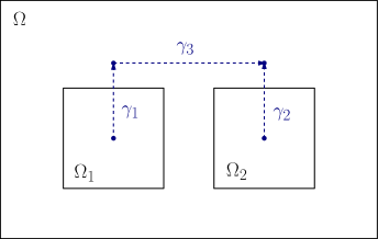
  Figure 3. Atomistic region with two components to visualise the argument given in §6.4.

  It is then reasonable to assume that the parameters $C_{x,r,s}$ have the same value in those parts of the interface surrounding $\Omega_{1}$ and $\Omega_{2}$, which would imply that

  $$\int_{\gamma_{1}}\Sigma_{\rm ac}(y_{\sf F})\cdot\,{\rm d}x=\int_{\gamma_{2}}\Sigma_{\rm ac}(y_{\sf F})\cdot\,{\rm d}x,$$

  Moreover, since $\Sigma_{\rm ac}(y_{\sf F})=\partial W({\sf F})$ in the continuum region, we would obtain that

  $$\int_{\gamma_{1}\cup\gamma_{3}\cup\gamma_{2}^{\prime}}\big{(}\Sigma_{\rm ac}(y_{\sf F})-\partial W({\sf F})\big{)}\cdot\,{\rm d}x=0,$$

  where $\gamma_{2}^{\prime}$ denotes the curve $\gamma_{2}$ with reversed orientation.

  This shows that it is possible to choose $\psi({\sf F};\cdot)=0$ in both components of $\Omega_{\rm a}$, and as a consequence, Theorem 6 would remain true.

A related issue is the dependence of the modelling error estimate (44) on ${\rm width}(\Omega_{\rm i})$, which comes solely from the Lipschitz estimate on ${\sf F}\mapsto\psi({\sf F};\cdot)$; cf. §6.3. Hence, a better understanding of this function may also allow a finer analysis of this undesirable dependence.

The global energy consistency condition

Global energy consistency is a natural and convenient condition that yields the important intermediate result (Corollary 6.2) that

$$\mathchoice{{\vbox{\hbox{$\textstyle-$ }}\kern-7.83337pt}}{{\vbox{\hbox{$\scriptstyle-$ }}\kern-5.90005pt}}{{\vbox{\hbox{$\scriptscriptstyle-$ }}\kern-4.75003pt}}{{\vbox{\hbox{$\scriptscriptstyle-$ }}\kern-4.25003pt}}\!\int_{\Omega}\Sigma_{\rm ac}(y_{\sf F})\,{\rm d}x=\partial W({\sf F})\qquad\forall\,{\sf F}\in\mathbb{R}^{2\times 2}.$$ (73)

Note also that (73) implies $\mathscr{E}_{\rm ac}(y_{\sf F})=\mathscr{E}_{\rm a}(y_{\sf F})+c$ for all ${\sf F}\in\mathbb{R}^{2\times 2}$, where $c$ is a fixed constant that is independent of ${\sf F}$; that is, (73) is practically equivalent to global energy consistency.

In some important situations patch test consistency already implies (73). The following result gives such a result for finite atomistic regions.

Proposition 21. Suppose that $\Omega_{\rm a}\cup\Omega_{\rm i}\subset{\rm int}(\Omega)$; then patch test consistency (14) of $\mathscr{E}_{\rm ac}$ implies (73).

Proof.

According to Lemmas 6.2 and 6.2 we have

$$\big{\langle}\delta\mathscr{E}_{\rm ac}(y_{\sf F}),u\big{\rangle}=\int_{\Omega_{\rm c}}\partial W({\sf F}):\nabla u\,{\rm d}x+\int_{\Omega_{\rm a}\cup\Omega_{\rm i}}\Sigma_{\rm ac}(y_{\sf F}):\nabla u\,{\rm d}x.$$

Let ${\sf G}\in\mathbb{R}^{2\times 2}$ and choose any $u\in\mathscr{U}$ such that $\nabla u={\sf G}$ in $\Omega_{\rm i}\cup\Omega_{\rm a}$; this is possible due to the assumption that $\Omega_{\rm a}\cup\Omega_{\rm i}\subset{\rm int}(\Omega)$. Integrating by parts twice, letting $\nu$ denote the unit outward normal to $\Omega_{\rm i}\cup\Omega_{\rm a}$, and noting that the portions of the surface integrals along $\partial\Omega$ cancel each other out, yields

$$\big{\langle}\delta\mathscr{E}_{\rm ac}(y_{\sf F}),u\big{\rangle}=~{} \int_{\Omega_{\rm c}}\partial W({\sf F}):\nabla u\,{\rm d}x+\int_{\Omega_{\rm a}\cup\Omega_{\rm i}}\Sigma_{\rm ac}(y_{\sf F}):{\sf G}\,{\rm d}x$$

$$=~{} -\int_{\partial(\Omega_{\rm a}\cup\Omega_{\rm i})}\partial W({\sf F}):(u\otimes\nu)\,{\rm d}s+\int_{\Omega_{\rm a}\cup\Omega_{\rm i}}\Sigma_{\rm ac}(y_{\sf F}):{\sf G}\,{\rm d}s$$

$$=~{} -\int_{\Omega_{\rm a}\cup\Omega_{\rm i}}\partial W({\sf F}):\nabla u\,{\rm d}x+\int_{\Omega_{\rm a}\cup\Omega_{\rm i}}\Sigma_{\rm ac}(y_{\sf F}):{\sf G}\,{\rm d}s$$

$$=~{} \int_{\Omega_{\rm a}\cup\Omega_{\rm i}}\big{[}\Sigma_{\rm ac}(y_{\sf F})-\partial W({\sf F})\big{]}:{\sf G}\,{\rm d}x.$$

Since $\mathscr{E}_{\rm ac}$ is patch test consistent, the last term vanishes, and hence the result follows. ∎

It turned out to be difficult to devise a counterexample, which clearly demonstrates that absence (73) can yield an inconsistent method. A more thorough investigation of this condition is still required.

The locality condition

To show that the locality condition (21) (or a variant thereof) is necessary we assume, without loss of generality, that $N$ is even and define a functional $\mathscr{J}\in{\rm C}^{2}(\mathscr{Y})$, $\mathscr{J}=\varepsilon^{2}J$,

$$J(y)=\bigg{|}\sum_{x\in\mathscr{L}^{\rm i}_{-,+}}\!\!D_{\!e_{1}}y(x)\bigg{|}^{2}+\bigg{|}\sum_{x\in\mathscr{L}^{\rm i}_{+,+}}\!\!D_{\!e_{1}}y(x)\bigg{|}^{2}-\bigg{|}\sum_{x\in\mathscr{L}^{\rm i}_{-,-}}\!\!D_{\!e_{1}}y(x)\bigg{|}^{2}-\bigg{|}\sum_{x\in\mathscr{L}^{\rm i}_{+,-}}\!\!D_{\!e_{1}}y(x)\bigg{|}^{2},$$

where,

$$\mathscr{L}^{\rm i}_{-,\pm}=~{} \big{\{}x\in\mathscr{L}\,\big{|}\,x_{1}\leq 0,x_{2}=\pm 1/2\big{\}},\quad\text{and}$$

$$\mathscr{L}^{\rm i}_{+,\pm}=~{} \big{\{}x\in\mathscr{L}\,\big{|}\,x_{1}>0,x_{2}=\pm 1/2\big{\}}.$$

From the definition it is obvious that $J(y_{\sf F})=0$ for all ${\sf F}\in\mathbb{R}^{2\times 2}$. Moreover, using summation by parts along the two lines $\mathscr{L}^{\rm i}_{-,+}\cup\mathscr{L}^{\rm i}_{+,+}$ and $\mathscr{L}^{\rm i}_{-,-}\cup\mathscr{L}^{\rm i}_{+,-}$, it is easy to check that the patch test (14) holds. Finally, $\mathscr{J}$ satisfies the scaling condition,

$$\partial_{(x,x+\varepsilon r)}\partial_{(x^{\prime},x^{\prime}+\varepsilon r)}J(y)=\left\{\begin{array}[]{rl}2\,{\sf I},&\text{if }r=e_{1}\text{ and }x,x^{\prime}\in\mathscr{L}^{\rm i}_{a,b},\quad a,b\in\{+,-\},\\ 0,&\text{otherwise}.\end{array}\right.$$

However, $\mathscr{J}$ clearly violates the locality condition.

We may think of $\mathscr{J}$ as an a/c functional for $\mathscr{E}_{\rm a}=0$, or, alternatively, as an additional contribution that can be added to any a/c functional whose interface satisfies $\mathscr{L}^{\rm i}_{-,+}\cup\mathscr{L}^{\rm i}_{-,-}\cup\mathscr{L}^{\rm i}_{+,+}\cup\mathscr{L}^{\rm i}_{+,-}\subset{\rm int}(\Omega_{\rm i}^{\#})$.

Let $y\in\mathscr{Y}_{\sf A}$ be “smooth” but not affine in the upper half plane $\{x\in\mathscr{L}\,|\,x_{2}\geq 0\}$, and let $y=y_{\sf A}$ on the lower interface $\mathscr{L}^{\rm i}_{-,-}\cup\mathscr{L}^{\rm i}_{+,-}$; then, testing $\delta\mathscr{J}(y)$ with the unique displacement $u\in\mathscr{U}$ such that

$$u(x)=y(x)-{\sf A}x \qquad\text{for }x\in\{(0,1/2),(1,1/2)\};$$

$$x_{1}\mapsto u(x_{1},1/2) [-1,0] [0,1]$$ is affine in and in ; and

$$D_{\!e_{2}}u(x)=0 \qquad\text{for all }x\in\mathscr{L};$$

then we obtain, after a brief computation,

$$\big{\|}\delta\mathscr{J}(y)\big{\|}_{{\rm W}^{-1,2}_{\varepsilon}}\geq\frac{\big{\langle}\delta\mathscr{J}(y),u\big{\rangle}}{\|\nabla u\|_{{\rm L}^{2}(\Omega)}}=\bigg{(}\Big{|}\varepsilon\!\!\sum_{x\in\mathscr{L}^{\rm i}_{-,+}}\!\!\big{(}D_{\!e_{1}}y(x)-{\sf A}e_{1}\big{)}\Big{|}^{2}+\Big{|}\varepsilon\!\!\sum_{x\in\mathscr{L}^{\rm i}_{+,+}}\!\!\big{(}D_{\!e_{1}}y(x)-{\sf A}e_{1}\big{)}\Big{|}^{2}\bigg{)}^{1/2}.$$

This final estimate is scaled like a surface integral and is clearly a zeroth order term if $y$ is smooth but $y(0,1/2)\neq y(1,1/2)$. This shows that the locality condition (21) (or a variant thereof) is indeed necessary to obtain a first-order consistency estimate.

The scaling condition

It is fairly clear that the modelling error estimate can be arbitrarily large without the scaling condition (22). We nevertheless briefly discuss a simple example with a natural interpretation.

Using a similar argument as in the previous paragraph, we define a functional $\mathscr{J}\in{\rm C}^{2}(\mathscr{Y})$, $\mathscr{J}=\varepsilon^{2}J$,

$$J(y)=\beta\sum_{x\in\mathscr{L}^{\rm i}_{+}}\big{|}D_{\!e_{1}}y(x)\big{|}^{2}-\beta\sum_{x\in\mathscr{L}^{\rm i}_{-}}\big{|}D_{\!e_{1}}y(x)\big{|}^{2},$$

where $\beta>0$ is a constant, and where

$$\mathscr{L}^{\rm i}_{\pm}=\big{\{}x\in\mathscr{L}\,\big{|}\,x_{2}=\pm 1/2\big{\}}.$$

It is easy to see that $J$ is patch test consistent, that $J(y_{\sf F})=0$ for all ${\sf F}\in\mathbb{R}^{2\times 2}$, and that it satisfies the locality condition.

Let $y\in\mathscr{Y}$ such that $y(x)={\sf A}x$ for $x_{2}=-1/2$, then testing $\delta\mathscr{J}(y)$ with the unique displacement $u\in\mathscr{U}$ such that

$$u(x)=y(x)-{\sf A}x, \quad\text{for }x\in\mathscr{L}^{\rm i}_{+},$$

$$D_{\!e_{2}}u(x)=0, \quad\text{for all }x\in\mathscr{L},$$

we obtain

$$\big{\|}\delta\mathscr{J}(y)\big{\|}_{{\rm W}^{-1,2}_{\varepsilon}}\geq\frac{\big{\langle}\delta\mathscr{J}(y),u\big{\rangle}}{\|\nabla u\|_{{\rm L}^{2}}}=\beta\varepsilon\bigg{[}\varepsilon\sum_{x\in\mathscr{L}^{\rm i}_{+}}\big{|}D_{\!e_{1}}y(x)-{\sf A}e_{1}\big{|}^{2}\bigg{]}^{1/2}.$$ (74)

If $y$ is “smooth” but not affine, then the term in square brackets is of the order $O(1)$. By choosing $\beta$ arbitrarily large, the modelling error can be made arbitrarily large as well. In particular, the choice $\beta=1/\varepsilon$ would give a seemingly natural surface scaling to the interface functional, and in this case we would obtain an $O(1)$ modelling error.

7. Conclusion

A fairly complete consistency analysis of general patch test consistent a/c coupling methods in (one and) two space dimensions was developed in this paper. The main result is the first order modelling error estimate, Theorem 6. The main undesirable condition is the assumption that ${\rm int}(\Omega_{\rm a})$ is connected. To remove this assumption a finer analysis of the corrector functions $\psi({\sf F},\cdot)$ defined in §6.2 is required. At this point one cannot exclude the possibility that a/c methods exist for which this assumption is in fact necessary.

Many open problems remain to be answered. First and foremost, one ought to answer the question whether a/c methods satisfying all the conditions of Theorem 6 always exist. In [45], we present a general construction (a variant on the geometrically consistent coupling method [15]) that appears to work in practise, however, we have no proof of this fact so far. Indeed, if it should turn out that in certain cases the “ghost forces” cannot be completely removed, then an extension of Theorem 6 estimating the contribution of the “ghost force” to the modelling error is highly desirable since such a result would provide the correct quantity that needs to be minimized. It is by no means clear that minimizing the “ghost force” itself is the best possible target. A similar analysis would also be useful for estimating the modelling error of blending methods [55].

It should be conceptually straightforward, though technically more demanding, to generalize all results to higher order finite element methods in the continuum region, however, it would then also be desirable to obtain the second order modelling error estimate in the continuum region. Such a result seems difficult to obtain without a more detailed understanding of the corrector functions $\psi({\sf F},\cdot)$.

An immediate question is whether a variant of the main result is still valid in 3D. This is by no means clear at this point. From a technical point of view, we require generalizations of the two main technical tools: the bond density lemma (§5.1) and the characterisation of discrete divergence-free ${\rm P}_{0}$-tensor fields (§5.2). While the bond density lemma as stated in this paper is false in 3D, one can establish variants that are potentially usefull for a 3D analysis (work in progress). Generalising the explicit construction of §5.2 is entirely open at this point.

Another important and difficult question is the extension to multi-lattices where the Cauchy–Born model is obtained through a homogenization procedure [1, 9].

Finally, it should be stressed, that Theorem 6 is a general abstract result, and as such can undoubtedly be improved upon when a specific coupling method is analyzed. It may be possible for specific methods to obtain more information about the corrector functions $\psi({\sf F},\cdot)$, and hence obtain a better estimate on the dependence of the modelling error on the interface width. For example, the consistency analysis in [41] requires no corrector functions at all, and in the consistency analysis of nearest-neighbour interactions [45] the corrector function vanishes in the continuum region. The proof of Theorem 6 may, however, serve as a general guidance for modelling error estimates in specific cases.

Finally, the stability of a/c methods in 2D/3D is largely open at this point.

Appendix A Proofs of §3

Proof of Lemma 3.1.

For $d=1$, since $I_{\varepsilon}y_{h}=y_{h}$, the result is trivial; hence assume that $d=2$. Assume also that $p<\infty$. Since the norms involved are effectively weighted $\ell^{p}$-norms, one can obtain the case $p=\infty$ as the limit $p\nearrow\infty$.

In this proof we will in fact use a periodic version of (40), which is a simple consequence of (40) (see also [41]):

$$|T|=\varepsilon^{2}\sum_{x\in\mathscr{L}}\mathchoice{{\vbox{\hbox{$\textstyle-$ }}\kern-7.83337pt}}{{\vbox{\hbox{$\scriptstyle-$ }}\kern-5.90005pt}}{{\vbox{\hbox{$\scriptscriptstyle-$ }}\kern-4.75003pt}}{{\vbox{\hbox{$\scriptscriptstyle-$ }}\kern-4.25003pt}}\!\int_{x}^{x+\varepsilon r}\chi_{T^{\#}}\,{\rm db}.$$

With our definition of the ${\rm L}^{p}$-norms for matrix-valued functions, we have

$$\big{\|}\nabla I_{\varepsilon}y_{h}\big{\|}_{{\rm L}^{p}(\Omega)}^{p}=\sum_{j=1}^{2}\int_{\Omega}\big{|}\nabla I_{\varepsilon}y_{h}e_{j}\big{|}_{p}^{p}\,{\rm d}x=\sum_{j=1}^{2}\int_{\Omega}\big{|}\nabla_{\!\!e_{j}}I_{\varepsilon}y_{h}\big{|}_{p}^{p}\,{\rm d}x.$$

Using the periodic bond density lemma, and the fact that $\{\chi_{T^{\#}}\,|\,T\in\mathscr{T}_{\varepsilon}\}$ is a partition of unity for $\mathbb{R}^{2}$, we have

$$\int_{\Omega}\big{|}\nabla_{\!\!e_{j}}I_{\varepsilon}y_{h}\big{|}_{p}^{p}\,{\rm d}x=~{} \sum_{T\in\mathscr{T}_{\varepsilon}}|T|\big{|}\nabla_{\!\!e_{j}}I_{\varepsilon}y_{h}(T)\big{|}_{p}^{p}$$

$$=~{} \sum_{T\in\mathscr{T}_{\varepsilon}}\big{|}\nabla_{\!\!e_{j}}I_{\varepsilon}y_{h}(T)\big{|}_{p}^{p}\varepsilon^{2}\sum_{x\in\mathscr{L}}\mathchoice{{\vbox{\hbox{$\textstyle-$ }}\kern-7.83337pt}}{{\vbox{\hbox{$\scriptstyle-$ }}\kern-5.90005pt}}{{\vbox{\hbox{$\scriptscriptstyle-$ }}\kern-4.75003pt}}{{\vbox{\hbox{$\scriptscriptstyle-$ }}\kern-4.25003pt}}\!\int_{x}^{x+\varepsilon e_{j}}\chi_{T^{\#}}\,{\rm db}$$

$$=~{} \varepsilon^{2}\sum_{x\in\mathscr{L}}\sum_{T\in\mathscr{T}_{\varepsilon}}\mathchoice{{\vbox{\hbox{$\textstyle-$ }}\kern-7.83337pt}}{{\vbox{\hbox{$\scriptstyle-$ }}\kern-5.90005pt}}{{\vbox{\hbox{$\scriptscriptstyle-$ }}\kern-4.75003pt}}{{\vbox{\hbox{$\scriptscriptstyle-$ }}\kern-4.25003pt}}\!\int_{x}^{x+\varepsilon e_{j}}\big{|}\nabla_{\!\!e_{j}}I_{\varepsilon}y_{h}\big{|}_{p}^{p}\chi_{T^{\#}}\,{\rm db}.$$

$$=~{} \varepsilon^{2}\sum_{x\in\mathscr{L}}\mathchoice{{\vbox{\hbox{$\textstyle-$ }}\kern-7.83337pt}}{{\vbox{\hbox{$\scriptstyle-$ }}\kern-5.90005pt}}{{\vbox{\hbox{$\scriptscriptstyle-$ }}\kern-4.75003pt}}{{\vbox{\hbox{$\scriptscriptstyle-$ }}\kern-4.25003pt}}\!\int_{x}^{x+\varepsilon e_{j}}\big{|}\nabla_{\!\!e_{j}}I_{\varepsilon}y_{h}\big{|}_{p}^{p}\,{\rm db}.$$ (75)

We have also used the fact that $\nabla_{\!\!e_{j}}I_{\varepsilon}y_{h}$ is continuous across edges that have direction $e_{j}$.

Due to the specific choice of the triangulation $\mathscr{T}_{\varepsilon}$ it follows that $\nabla_{\!\!e_{j}}I_{\varepsilon}y_{h}$ is constant along each bond $(x,x+\varepsilon e_{j})$, and hence

$$\mathchoice{{\vbox{\hbox{$\textstyle-$ }}\kern-7.83337pt}}{{\vbox{\hbox{$\scriptstyle-$ }}\kern-5.90005pt}}{{\vbox{\hbox{$\scriptscriptstyle-$ }}\kern-4.75003pt}}{{\vbox{\hbox{$\scriptscriptstyle-$ }}\kern-4.25003pt}}\!\int_{x}^{x+\varepsilon e_{j}}\big{|}\nabla_{\!\!e_{j}}I_{\varepsilon}y_{h}\big{|}_{p}^{p}\,{\rm db}=\big{|}D_{\!e_{j}}I_{\varepsilon}y_{h}(x)\big{|}_{p}^{p}=\bigg{|}\mathchoice{{\vbox{\hbox{$\textstyle-$ }}\kern-7.83337pt}}{{\vbox{\hbox{$\scriptstyle-$ }}\kern-5.90005pt}}{{\vbox{\hbox{$\scriptscriptstyle-$ }}\kern-4.75003pt}}{{\vbox{\hbox{$\scriptscriptstyle-$ }}\kern-4.25003pt}}\!\int_{x}^{x+\varepsilon e_{j}}\nabla_{\!\!e_{j}}y_{h}\,{\rm db}\bigg{|}_{p}^{p}\leq\mathchoice{{\vbox{\hbox{$\textstyle-$ }}\kern-7.83337pt}}{{\vbox{\hbox{$\scriptstyle-$ }}\kern-5.90005pt}}{{\vbox{\hbox{$\scriptscriptstyle-$ }}\kern-4.75003pt}}{{\vbox{\hbox{$\scriptscriptstyle-$ }}\kern-4.25003pt}}\!\int_{x}^{x+\varepsilon e_{j}}\big{|}\nabla_{\!\!e_{j}}y_{h}\big{|}_{p}^{p}\,{\rm db},$$

where we employed Jensen’s inequality in the last step.

Inserting this estimate into (75), and reversing the argument in (75), we arrive at

$$\int_{\Omega}\big{|}\nabla_{\!\!e_{j}}I_{\varepsilon}y_{h}\big{|}_{p}^{p}\,{\rm d}x\leq~{} \varepsilon^{2}\sum_{x\in\mathscr{L}}\mathchoice{{\vbox{\hbox{$\textstyle-$ }}\kern-7.83337pt}}{{\vbox{\hbox{$\scriptstyle-$ }}\kern-5.90005pt}}{{\vbox{\hbox{$\scriptscriptstyle-$ }}\kern-4.75003pt}}{{\vbox{\hbox{$\scriptscriptstyle-$ }}\kern-4.25003pt}}\!\int_{x}^{x+\varepsilon e_{j}}\big{|}\nabla_{\!\!e_{j}}y_{h}\big{|}_{p}^{p}\,{\rm db}$$

$$=~{} \sum_{T\in\mathscr{T}_{h}}\varepsilon^{2}\sum_{x\in\mathscr{L}}\mathchoice{{\vbox{\hbox{$\textstyle-$ }}\kern-7.83337pt}}{{\vbox{\hbox{$\scriptstyle-$ }}\kern-5.90005pt}}{{\vbox{\hbox{$\scriptscriptstyle-$ }}\kern-4.75003pt}}{{\vbox{\hbox{$\scriptscriptstyle-$ }}\kern-4.25003pt}}\!\int_{x}^{x+\varepsilon e_{j}}\big{|}\nabla_{\!\!e_{j}}y_{h}\big{|}_{p}^{p}\chi_{T^{\#}}\,{\rm db}$$

$$=~{} \sum_{T\in\mathscr{T}_{h}}|T|\,\big{|}\nabla_{\!\!e_{j}}y_{h}(T)\big{|}_{p}^{p}=\big{\|}\nabla_{\!\!e_{j}}y_{h}\big{\|}_{{\rm L}^{p}(\Omega)}^{p}.\qed$$

Remark 9. From the foregoing proof, it follows that

$$\big{\|}\nabla y\big{\|}_{{\rm L}^{p}(\Omega)}=\bigg{(}\varepsilon^{2}\sum_{j=1}^{2}\sum_{x\in\mathscr{L}}\big{|}D_{\!e_{j}}y(x)\big{|}_{p}^{p}\bigg{)}^{1/p}\qquad\text{for }y\in\mathscr{Y}.\qed$$

Proof of Lemma 3.2.

To simplify the notation, we define the scalar function $z=y_{i}$ for some fixed $i$. Moreover, we prove the result only for $d=2$; for $d=1$ the result follows from the interpolation error estimates established in [42].

Step 1. ${\rm W}^{2,\infty}$-interpolant: We first define a ${\rm W}^{2,\infty}$-interpolant $\tilde{z}$ of $z$, using the ${\rm C}^{1}$-conforming Hsieh–Clough–Tocher (HCT) element [7]; see Figure 4.

Figure 4. Illustration of the degrees of freedom in the ${\rm C}^{1}$-conforming Clough–Tocher element: black dots denote point values, circles denote gradient values, arrows denote directional derivatives.

Let $T\in\mathscr{T}_{\varepsilon}^{\rm c}$ and let $Q_{T}$ denote the set of vertices of $T$, and $F_{T}$ the set of edges of $T$.

For each vertex $q\in Q_{T}$, we define the point value $\tilde{z}(q)=z(q)$, and the gradient value by $\nabla\tilde{z}(q)=\mathchoice{{\vbox{\hbox{$\textstyle-$ }}\kern-7.83337pt}}{{\vbox{\hbox{$\scriptstyle-$ }}\kern-5.90005pt}}{{\vbox{\hbox{$\scriptscriptstyle-$ }}\kern-4.75003pt}}{{\vbox{\hbox{$\scriptscriptstyle-$ }}\kern-4.25003pt}}\!\int_{\omega_{q}^{\rm c}}\nabla z\,{\rm d}x$, where

$$\omega_{q}^{\rm c}=\bigcup\big{\{}T^{\prime}\in(\mathscr{T}_{\varepsilon}^{\rm c})^{\#}\,\big{|}\,q\in T^{\prime}\big{\}}.$$

Similarly, for each edge $f\in F_{T}$, $f=T\cap T^{\prime}$, with midpoint $q_{f}$, we define the patch $\omega_{f}^{\rm c}=\Omega_{\rm c}^{\#}\cap(T\cup T^{\prime})$, and the directional derivative $\nabla_{\!\!\nu}\tilde{z}(q_{f})=\mathchoice{{\vbox{\hbox{$\textstyle-$ }}\kern-7.83337pt}}{{\vbox{\hbox{$\scriptstyle-$ }}\kern-5.90005pt}}{{\vbox{\hbox{$\scriptscriptstyle-$ }}\kern-4.75003pt}}{{\vbox{\hbox{$\scriptscriptstyle-$ }}\kern-4.25003pt}}\!\int_{\omega_{f}^{\rm c}}\nabla_{\!\!\nu}z\,{\rm d}x$.

Let $\varphi_{q}$ be the nodal basis function associated with the point value at a vertex $q$, $\phi_{f}$ the nodal basis function associated with the normal derivative at an edge $f$, and let $\Phi_{q,\alpha}$ be the nodal basis function associated with the $\alpha$-component of the derivative $\nabla z(q)$.

Step 2. Estimating $z-\tilde{z}$: Fix $T\in\mathscr{T}_{\varepsilon}^{\rm c}$, $x\in T$, and define ${\sf F}=\nabla z(T)$, then we have

$$\big{|}\nabla z(T)-\nabla\tilde{z}(x)\big{|}=~{} \big{|}{\sf F}-\nabla\tilde{z}(x)\big{|}$$

$$\leq~{} \bigg{|}\sum_{f\in F_{T}}\big{(}{\sf F}\cdot\nu_{f}-\nabla_{\!\!\nu_{f}}\tilde{z}(q_{f})\big{)}\otimes\nabla\varphi_{f}(x)\bigg{|}+\bigg{|}\sum_{\begin{subarray}{c}q\in Q_{T}\\ \alpha\in\{1,2\}\end{subarray}}\big{(}{\sf F}_{\alpha}-\partial_{x_{\alpha}}\tilde{z}(q)\big{)}\otimes\nabla\Phi_{q,\alpha}\bigg{|}.$$

Since all elements $T\in\mathscr{T}_{\varepsilon}$ are translated, scaled, and possibly reflected, copies of the reference triangle $\hat{T}={\rm conv}\{(0,0),(1,0),(0,1)\}$, it follows that the HCT nodal basis functions are given (up to translations and reflections) by

$$\varphi_{f}(x)=\varepsilon\hat{\varphi}_{f}\big{(}\varepsilon^{-1}x\big{)},\quad\text{and}\quad\hat{\Phi}_{q,\alpha}(x)=\varepsilon\Phi_{q,\alpha}\big{(}\varepsilon^{-1}x\big{)}.$$

Note in particular, that the gradients of these nodal basis functions are scale invariant, that is,

$$\|\nabla\varphi_{f}\|_{{\rm L}^{\infty}}\leq C\quad\text{and}\quad\|\nabla\Phi_{q,\alpha}\|_{{\rm L}^{\infty}}\leq C,$$

where $C$ is a fixed constant that is independent of $\varepsilon$.

From the construction of $\tilde{z}$ it is easy to see that, for $f\in F_{q},q\in Q_{T},\alpha\in\{1,2\}$,

$$\big{|}{\sf F}\nu_{f}-\nabla_{\!\!\nu_{f}}\tilde{z}(q_{f})\big{|}\leq\varepsilon\,{\rm osc}(\nabla z;\omega_{T}^{\rm c}),\quad\text{and}\quad\big{|}{\sf F}_{\alpha}-\partial_{x_{\alpha}}\tilde{z}(q)\big{|}\leq\varepsilon\,{\rm osc}(\nabla z;\omega_{T}^{\rm c});$$

and hence we obtain

$$\big{\|}\nabla z(T)-\nabla\tilde{z}\big{\|}_{{\rm L}^{p}(T)}\leq C_{1}\varepsilon\,|T|^{1/p}\,{\rm osc}(\nabla z;\omega_{T}^{\rm c}),$$ (76)

for some generic constant $C_{1}$.

Step 3. Interpolation error: Using standard interpolation error estimates [7], we obtain

$$\big{\|}\nabla\tilde{z}-\nabla I_{h}\tilde{z}\big{\|}_{{\rm L}^{p}(\Omega_{\rm c})}\leq C_{I}^{\prime}\big{\|}h\nabla^{2}\tilde{z}\big{\|}_{{\rm L}^{p}(\Omega_{\rm c})}.$$

Let $T\in\mathscr{T}_{\varepsilon}$ and ${\sf F}=\nabla z(T)$, then application of an inverse inequality, and (76) yield

$$\big{\|}\nabla^{2}\tilde{z}\big{\|}_{{\rm L}^{p}(T)}=~{} \big{\|}\nabla^{2}(\tilde{z}-z)\big{\|}_{{\rm L}^{p}(T)}\leq C_{2}\varepsilon^{-1}\big{\|}\nabla\tilde{z}-{\sf F}\big{\|}_{{\rm L}^{p}(T)}\leq C_{2}\,|T|^{1/p}\,{\rm osc}(\nabla z;\omega_{T}^{\rm c}).$$ (77)

Finally, since $\tilde{z}(x)=z(x)$ for all $x\in\mathscr{L}^{\#}$, it follows that $I_{h}z=I_{h}\tilde{z}$, and hence we can estimate

$$\big{\|}\nabla z-\nabla I_{h}z\big{\|}_{{\rm L}^{p}(\Omega)}=~{} \big{\|}\nabla z-\nabla I_{h}z\big{\|}_{{\rm L}^{p}(\Omega_{\rm c})}$$

$$\leq~{} \big{\|}\nabla z-\nabla\tilde{z}\big{\|}_{{\rm L}^{p}(\Omega_{\rm c})}+\big{\|}\nabla\tilde{z}-\nabla I_{h}\tilde{z}\big{\|}_{{\rm L}^{p}(\Omega_{\rm c})}.$$

Employing (76) and (77), we obtain the stated result. ∎

Proof of Lemma 3.5.

For each $f\in\mathscr{F}_{\varepsilon}$, let $f=T_{-}\cap T_{+}$, $T_{\pm}\in\mathscr{T}_{\varepsilon}$, let $\nu_{\pm}$ denote the corresponding unit outward normals, and $\omega_{f}^{\prime}=T_{+}\cup T_{-}$.

We integrate by parts in each element $T\in\mathscr{T}_{\varepsilon}$ and use the fact that $I_{\varepsilon}u_{h}=u_{h}$ in $\Omega_{\rm i}\cup\Omega_{\rm a}$ to obtain

$$\Big{|}\big{\langle}\Phi,I_{\varepsilon}u_{h}\big{\rangle}-\big{\langle}\Phi_{h},u_{h}\big{\rangle}\Big{|}=~{} \bigg{|}\sum_{T\in\mathscr{T}_{\varepsilon}}\int_{T}\sigma(T):\nabla\big{(}I_{\varepsilon}u_{h}-u_{h}\big{)}\,{\rm d}x\bigg{|}$$

$$=~{} \bigg{|}\sum_{\begin{subarray}{c}f\in\mathscr{F}_{\varepsilon}\\ f\not\subset\Omega_{\rm i}\cup\Omega_{\rm a}\end{subarray}}\int_{f}\big{(}\sigma(T_{+})\nu_{+}+\sigma(T_{-})\nu_{-}\big{)}\cdot\big{(}I_{\varepsilon}u_{h}-u_{h}\big{)}\,{\rm d}s\bigg{|}$$

$$\leq~{} \sum_{\begin{subarray}{c}f\in\mathscr{F}_{\varepsilon}\\ f\not\subset\Omega_{\rm i}\cup\Omega_{\rm a}\end{subarray}}\varepsilon{\rm osc}(\sigma;\omega_{f}^{\prime})\,\int_{f}\big{|}I_{\varepsilon}u_{h}-u_{h}\big{|}\,{\rm d}s.$$ (78)

Let $v:=I_{\varepsilon}u_{h}-u_{h}$. An application of [39, Lemma 6.6] yields the trace inequality

$$\|v\|_{{\rm L}^{1}(f)}\leq\varepsilon^{-1}\|v\|_{{\rm L}^{1}(\omega_{f}^{\prime})}+\|\nabla v\|_{{\rm L}^{1}(\omega_{f}^{\prime})}.$$ (79)

Furthermore, since $v$ is Lipschitz continuous and $v(p)=0$ on every vertex of the triangulation $\mathscr{T}_{\varepsilon}$, we can use [39, Lemma 6.8] to deduce that

$$\|v\|_{{\rm L}^{1}(\omega_{f}^{\prime})}\leq\sqrt{2}\varepsilon\|\nabla v\|_{{\rm L}^{1}(\omega_{f}^{\prime})}.$$ (80)

Combining (80), (79), and (78), applying two Hölder inequalities, and estimating the overlaps between the patches $\omega_{f}^{\prime}$, we deduce that

$$\Big{|}\big{\langle}\Phi,I_{\varepsilon}u_{h}\big{\rangle}-\big{\langle}\Phi_{h},u_{h}\big{\rangle}\Big{|}\leq~{} (1+\sqrt{2})\varepsilon\sum_{\begin{subarray}{c}f\in\mathscr{F}_{\varepsilon}\\ f\not\subset\Omega_{\rm i}\cup\Omega_{\rm a}\end{subarray}}{\rm osc}(\sigma;\omega_{f}^{\prime})|\omega_{f}^{\prime}|^{1/p}\big{\|}\nabla v\big{\|}_{{\rm L}^{p^{\prime}}(\omega_{f}^{\prime})}$$

$$\leq~{} C_{1}\varepsilon\bigg{(}\sum_{T\in\mathscr{T}^{\rm c}_{h}}|T|{\rm osc}(\sigma;\omega_{T}^{\rm c})^{p}\bigg{)}^{1/p}\big{\|}\nabla v\big{\|}_{{\rm L}^{p^{\prime}}(\Omega_{\rm c})}.$$

An application of Lemma 3.1 yields the stated result. ∎

Appendix B List of Symbols

$a\cdot b$, $a\otimes b$		vector dot product and tensor product; §1.3
$|\cdot|,|\cdot|_{p}$		$\ell^{p}$-norms; §1.3
$\|\cdot\|_{\ell^{p}_{\varepsilon}}$		weighted $\ell^{p}$-norms; §1.3
$\mathscr{L},\mathscr{L}^{\#}$		Lattice and lattice domain; §2.1
$y_{\sf A}$		homogeneous deformation; §2.1
$\mathscr{U},\mathscr{Y},\mathscr{Y}_{\sf A}$		spaces of periodic displacements and deformations §2.1
$A^{\#},\mathscr{A}^{\#}$		periodic extension of a set or family of sets §2.1
$\mathscr{R}$		interaction range, §2.1
$D_{\!r},D_{\!\mathscr{R}}$		finite difference operator and stencil §2.1
$\nabla_{\!\!r},\nabla$		directional derivative, deformation or displacement gradient, §1.3
$\partial v$		Jacobi matrix of vector valued function, §1.3
$\mathscr{E}_{\rm a}$		atomistic energy, §2.1
$V$		atomistic interaction potential, §2.1
$\mathscr{P}_{\rm a}$		external potential in atomistic model, §2.1
$\delta\mathscr{E}$, $\delta^{2}\mathscr{E}$, $\langle\cdot,\cdot\rangle$		first and second variations, abstract duality pairing, §2.1
$\partial_{r}V,\partial_{r,s}V$		first and second partial derivatives of $V$, §2.1
$M_{r,s}^{\rm a},M^{\rm a}$		bounds on $\partial_{r,s}V$ and Lipschitz constant for $\delta\mathscr{E}_{\rm a}$, §2.1
$\mathscr{T}_{h},\mathscr{T}_{h}^{\#},\mathscr{F}_{h},\mathscr{F}_{h}^{\#}$		triangulations, and edge sets, §2.3
$h_{T},h(x)$		mesh size functions, §2.3
${\rm P}_{1},{\rm P}_{0},{\rm P}_{1}^{\#},{\rm P}_{0}^{\#}$		finite element spaces, §2.3
$\mathscr{U}_{h},\mathscr{Y}_{h},\mathscr{Y}_{{\sf A},h}$		finite element spaces, §2.3
$I_{h}$		nodal interpolation operator for ${\rm P}_{1}(\mathscr{T}_{h})$, §2.3
$W$		Cauchy–Born stored energy function, §2.3
$\mathscr{E}_{\rm ac}$, $\mathscr{P}_{\rm ac}$		a/c energy and external potential, §2.3
$\Omega_{\rm a},\Omega_{\rm c},\Omega_{\rm i}$		atomistic, continuum, and interface region, §2.3
$\mathscr{T}_{h}^{\rm a},\mathscr{T}^{\rm c}_{h},\mathscr{T}^{\rm i}_{h}$		atomistic, continuum, and interface triangulations, §2.3
$\mathscr{L}_{\rm a}$		set of atomistic sites in a/c method, §2.3
$(x,x^{\prime}),(x,x+\varepsilon r)$		bonds, §2.3
$\mathscr{B}_{\rm i}$, $\mathscr{B}_{\rm i}^{\#}$		set of interface bonds, §2.3
$\mathscr{E}_{\rm i}$, $E_{\rm i}$		interface functional, §2.3
$\partial_{b}E_{\rm i},\partial_{(x,x+\varepsilon r)}E_{\rm i}$		scaled first partial derivatives of $E_{\rm i}$, §2.3
$M_{r,s}^{\rm i}$, $M^{\rm i}$		bounds on second partial derivatives of $E_{\rm i}$, §2.3
$\mathscr{T}_{\varepsilon},\mathscr{T}_{\varepsilon}^{\#},\mathscr{F}_{\varepsilon},\mathscr{F}_{\varepsilon}^{\#}$		atomistic triangulation and edge sets, §3.1
${\rm osc}$		oscillation operator, §3.1
$I_{\varepsilon}$		nodal interpolation operator for ${\rm P}_{1}(\mathscr{T}_{\varepsilon})$, §3.1
$\omega_{T}^{\rm c}$		patch used in the interpolation error estimate, §3.2
${\rm h}_{T}$		modified mesh size function §3.2
$\|\cdot\|_{{\rm W}^{-1,p}_{h}}$		${\rm W}^{1,p^{\prime}}$-dual norm on ${\rm P}_{1}(\mathscr{T}_{h})^{*}$, §3.4
$\|\cdot\|_{{\rm W}^{-1,p}_{\varepsilon}}$		${\rm W}^{1,p^{\prime}}$-dual norm on ${\rm P}_{1}(\mathscr{T}_{\varepsilon})^{*}$, §3.5
$\phi_{1},\phi_{2}$		first and second neighbour potential, §4
$x_{n},v_{n},v_{n}^{\prime},v_{n}^{\prime\prime},v_{n}^{\prime\prime\prime}$		notation for 1D grid functions, §4
$\chi_{T}$		characteristic function used in bond density lemma, §5.1
$\chi_{T}^{\rm i}$		characteristic function used to define $\Sigma_{\rm ac}$, Prop. 6.2, p.6.2
$\mathchoice{{\vbox{\hbox{$\textstyle-$ }}\kern-7.83337pt}}{{\vbox{\hbox{$\scriptstyle-$ }}\kern-5.90005pt}}{{\vbox{\hbox{$\scriptscriptstyle-$ }}\kern-4.75003pt}}{{\vbox{\hbox{$\scriptscriptstyle-$ }}\kern-4.25003pt}}\!\int_{x}^{x^{\prime}}f\,{\rm db},\mathchoice{{\vbox{\hbox{$\textstyle-$ }}\kern-7.83337pt}}{{\vbox{\hbox{$\scriptstyle-$ }}\kern-5.90005pt}}{{\vbox{\hbox{$\scriptscriptstyle-$ }}\kern-4.75003pt}}{{\vbox{\hbox{$\scriptscriptstyle-$ }}\kern-4.25003pt}}\!\int_{x}^{x+\varepsilon r}f\,{\rm db}$		bond integrals, §5.1
${\rm N}_{1}$, ${\rm N}_{1}^{\#}$		Crouzeix–Raviart finite element spaces, §5.2
$q_{f}$, $\zeta_{f}$, $\zeta_{f}^{\#}$		midpoint of an edge $f$ and associated nodal basis, §5.2
$\int_{\gamma}\sigma\cdot\,{\rm d}x$		path integral, §5.2
${\sf J}$		rotation about $\pi/2$, Lemma 5.2, p.5.2
$\omega_{T}^{\rm a},\omega_{T}$		atomistic interaction neighbourhoods, §6
$M_{T}$		prefactors in modelling error estimate, Eq. (45), p.45
${\rm width}(\Omega_{\rm i})$		width of $\Omega_{\rm i}$, Eq. (46), p.46
$\Sigma_{\rm a}$		atomistic stress function, Eq. (49), p.49
$V_{x,r},V_{{\sf F},r}$		alternative notation for $\partial_{r}V(D_{\!\mathscr{R}}y(x))$ and for $\partial_{r}V({\sf F}\mathscr{R})$
$\Sigma_{\rm ac}$		a/c stress function, Prop. 6.2, p.6.2
$\psi({\sf F};\cdot)$		corrector function for $\Sigma_{\rm ac}(y_{\sf F})$, Lemma 6.2, p.6.2
$\hat{\psi}(y;\cdot)$		corrector function for $\Sigma_{\rm ac}(y)$, Eq. (58), p.58
$\widehat{\Sigma}_{\rm ac}$		modified a/c stress function, Eq. (59), p. 59
${\sf R}(y;T)$		stress error, Eq. (63), p. 63

References

• [1] A. Abdulle, P. Lin, and A. Shapeev. Homogenization-based analysis of quasicontinuum method for complex crystals. arXiv:1006.0378.
• [2] N.C. Admal and E.B. Tadmor. A unified interpretation of stress in molecular systems. J. of Elasticity, 100:63–143, 2010.
• [3] R. Alicandro and M. Cicalese. A general integral representation result for continuum limits of discrete energies with superlinear growth. SIAM J. Math. Anal., 36(1):1–37 (electronic), 2004.
• [4] S. Badia, M. Parks, P. Bochev, M. Gunzburger, and R. Lehoucq. On atomistic-to-continuum coupling by blending. Multiscale Model. Simul., 7(1):381–406, 2008.
• [5] G. P. Bazeley, Y. K. Cheung, B. M. Irons, and 0. C. Zienkiewicz. Triangle elements in plate bending: conforming and nonconforming solutions. Proc. Conf. Matrix Meth. Struc. Mech., Ohio, 1966. Wright Patterson AFB.
• [6] Ted Belytschko, Wing Kam Liu, and Brian Moran. Nonlinear finite elements for continua and structures. John Wiley & Sons Ltd., Chichester, 2000.
• [7] P. G. Ciarlet. The finite element method for elliptic problems, volume 40 of Classics in Applied Mathematics. Society for Industrial and Applied Mathematics (SIAM), Philadelphia, PA, 2002. Reprint of the 1978 original [North-Holland, Amsterdam; MR0520174 (58 #25001)].
• [8] M. Dobson. work in progress.
• [9] M. Dobson, R. Elliot, M. Luskin, and E. Tadmor. A multilattice quasicontinuum for phase transforming materials: Cascading cauchy born kinematics. Journal of Computer-Aided Materials Design, 14:219–237, 2007.
• [10] M. Dobson and M. Luskin. Analysis of a force-based quasicontinuum approximation. M2AN Math. Model. Numer. Anal., 42(1):113–139, 2008.
• [11] M. Dobson and M. Luskin. An analysis of the effect of ghost force oscillation on quasicontinuum error. M2AN Math. Model. Numer. Anal., 43(3):591–604, 2009.
• [12] M. Dobson and M. Luskin. An optimal order error analysis of the one-dimensional quasicontinuum approximation. SIAM Journal on Numerical Analysis, 47(4):2455–2475, 2009.
• [13] M. Dobson, M. Luskin, and C. Ortner. Accuracy of quasicontinuum approximations near instabilities, 2010.
• [14] M. Dobson, M. Luskin, and C. Ortner. Stability, instability, and error of the force-based quasicontinuum approximation. Arch. Ration. Mech. Anal., 197(1):179–202, 2010.
• [15] W. E, J. Lu, and J.Z. Yang. Uniform accuracy of the quasicontinuum method. Phys. Rev. B, 74(21):214115, 2006.
• [16] W. E and P. Ming. Analysis of the local quasicontinuum method. In Frontiers and prospects of contemporary applied mathematics, volume 6 of Ser. Contemp. Appl. Math. CAM, pages 18–32. Higher Ed. Press, Beijing, 2005.
• [17] W. E and P. Ming. Cauchy-Born rule and the stability of crystalline solids: static problems. Arch. Ration. Mech. Anal., 183(2):241–297, 2007.
• [18] Bernhard Eidel and Alexander Stukowski. A variational formulation of the quasicontinuum method based on energy sampling in clusters. J. Mech. Phys. Solids, 57(1):87–108, 2009.
• [19] M. Finnis. Interatomic Forces in Condensed Matter, volume 1 of Oxford Series on Materials Modelling. Oxford University Press, 2003.
• [20] J. Fish, M. A. Nuggehally, M. S. Shephard, C. R. Picu, S. Badia, M. L. Parks, and M. Gunzburger. Concurrent AtC coupling based on a blend of the continuum stress and the atomistic force. Comput. Methods Appl. Mech. Engrg., 196(45-48):4548–4560, 2007.
• [21] Max Gunzburger and Yanzhi Zhang. A quadrature-rule type approximation to the quasi-continuum method. Multiscale Model. Simul., 8(2):571–590, 2009/10.
• [22] M. Iyer and V. Gavini. A field theoretic approach to the quasi-continuum method. to appear in J. Mech. Phys. Solids.
• [23] P. A. Klein and J. A. Zimmerman. Coupled atomistic-continuum simulations using arbitrary overlapping domains. J. Comput. Phys., 213(1):86–116, 2006.
• [24] J. Knap and M. Ortiz. An Analysis of the Quasicontinuum Method. J. Mech. Phys. Solids, 49:1899–1923, 2001.
• [25] S. Kohlhoff and S. Schmauder. A new method for coupled elastic-atomistic modelling. In V. Vitek and D. J. Srolovitz, editors, Atomistic Simulation of Materials: Beyond Pair Potentials, pages 411–418. Plenum Press, New York, 1989.
• [26] X. H. Li and M. Luskin. An analysis of the quasi-nonlocal quasicontinuum approximation of the embedded atom model. arXiv:1008.3628.
• [27] X. H. Li and M. Luskin. A generalized quasi-nonlocal atomistic-to-continuum coupling method with finite range interaction. arXiv:1007.2336.
• [28] P. Lin. Theoretical and numerical analysis for the quasi-continuum approximation of a material particle model. Math. Comp., 72(242):657–675, 2003.
• [29] P. Lin. Convergence analysis of a quasi-continuum approximation for a two-dimensional material without defects. SIAM J. Numer. Anal., 45(1):313–332 (electronic), 2007.
• [30] J. Lu and P. Ming. Convergence of a force-based hybrid method for atomistic and continuum models in three dimension. arXiv:1102.2523.
• [31] M. Luskin and C. Ortner. An analysis of node-based cluster summation rules in the quasicontinuum method. SIAM Journal on Numerical Analysis, 47(4):3070–3086, 2009.
• [32] C. Makridakis, C. Ortner, and E. Süli. Analysis of two force-based atomistic/continuum hybrid models of a periodic chain, 2010. OxMOS Report No. 28, Mathematical Institute, University of Oxford, UK.
• [33] C. Makridakis, C. Ortner, and E. Süli. Stress-based atomistic/continuum coupling: A new variant of the quasicontinuum approximation, 2010. OxMOS Preprint no. 27, Mathematical Institute, University of Oxford, UK.
• [34] R. Miller and E. Tadmor. A unified framework and performance benchmark of fourteen multiscale atomistic/continuum coupling methods. Modelling Simul. Mater. Sci. Eng., 17, 2009.
• [35] R.E. Miller and E.B. Tadmor. The Quasicontinuum Method: Overview, Applications and Current Directions. Journal of Computer-Aided Materials Design, 9:203–239, 2003.
• [36] P. Ming and J. Z. Yang. Analysis of a one-dimensional nonlocal quasi-continuum method. Multiscale Modeling & Simulation, 7(4):1838–1875, 2009.
• [37] M. Ortiz, R. Phillips, and E. B. Tadmor. Quasicontinuum analysis of defects in solids. Philosophical Magazine A, 73(6):1529–1563, 1996.
• [38] C. Ortner. unpublished notes.
• [39] C. Ortner. Analysis of the Quasicontinuum Method. PhD thesis, University of Oxford, 2006.
• [40] C. Ortner. A priori and a posteriori analysis of the quasi-nonlocal quasicontinuum method in 1d, 2009. arXiv.org:0911.0671v1, to appear in Math. Comp.
• [41] C. Ortner and A. Shapeev. Analysis of an energy-based quasicontinuum approximation of a vacancy in the 2d hexagonal lattice. in preparation.
• [42] C. Ortner and E. Süli. Analysis of a quasicontinuum method in one dimension. M2AN Math. Model. Numer. Anal., 42(1):57–91, 2008.
• [43] C. Ortner and H. Wang. Coarse graining in energy-based quasicontinuum methods. OxMOS Report No. 30, Mathematical Institute, University of Oxford, UK, 2010.
• [44] C. Ortner and L. Zhang. manuscript.
• [45] C. Ortner and L. Zhang. work in progress.
• [46] M. L. Parks, P. B. Bochev, and R. B. Lehoucq. Connecting atomistic-to-continuum coupling and domain decomposition. Multiscale Model. Simul., 7(1):362–380, 2008.
• [47] D. Pettifor. Bonding and structure of molecules and solids. Oxford University Press, 1995.
• [48] Konrad Polthier and Eike Preuß. Identifying vector field singularities using a discrete Hodge decomposition. In Visualization and mathematics III, Math. Vis., pages 113–134. Springer, Berlin, 2003.
• [49] A. Shapeev. Consistent energy-based atomistic/continuum coupling for two-body potential: 1d and 2d case. arXiv:1010.0512.
• [50] V. B. Shenoy, R. Miller, E. B. Tadmor, D. Rodney, R. Phillips, and M. Ortiz. An adaptive finite element approach to atomic-scale mechanics–the quasicontinuum method. J. Mech. Phys. Solids, 47(3):611–642, 1999.
• [51] L. E. Shilkrot, R. E. Miller, and W. A. Curtin. Coupled atomistic and discrete dislocation plasticity. Phys. Rev. Lett., 89(2):025501, 2002.
• [52] T. Shimokawa, J.J. Mortensen, J. Schiotz, and K.W. Jacobsen. Matching conditions in the quasicontinuum method: Removal of the error introduced at the interface between the coarse-grained and fully atomistic region. Phys. Rev. B, 69(21):214104, 2004.
• [53] Gilbert Strang and George Fix. An Analysis of the Finite Element Method. Wellesley-Cambridge Press, 2008.
• [54] B. Van Koten, Z. H. Li, M. Luskin, and C. Ortner. A computational and theoretical investigation of the accuracy of quasicontinuum methods. arXiv:1012.6031.
• [55] B. Van Koten and M. Luskin. Development and analysis of blended quasicontinuum approximations. arXiv:1008.2138.
• [56] S. P. Xiao and T. Belytschko. A bridging domain method for coupling continua with molecular dynamics. Comput. Methods Appl. Mech. Engrg., 193(17-20):1645–1669, 2004.