Asymptotic Equivalence for Nonparametric Regression with Non-Regular Errors

Alexander Meister		Markus Reiß
Institut für Mathematik		Institut für Mathematik
Universität Rostock		Humboldt-Universität zu Berlin
Ulmenstraße 69		Unter den Linden 6
18051 Rostock, Germany		10099 Berlin, Germany
e-mail: alexander.meister@uni-rostock.de		e-mail: mreiss@math.hu-berlin.de

Asymptotic equivalence in Le Cam’s sense for nonparametric regression experiments is extended to the case of non-regular error densities, which have jump discontinuities at their endpoints. We prove asymptotic equivalence of such regression models and the observation of two independent Poisson point processes which contain the target curve as the support boundary of its intensity function. The intensity of the point processes is of order of the sample size $n$ and involves the jump sizes as well as the design density. The statistical model significantly differs from regression problems with Gaussian or regular errors, which are known to be asymptotically equivalent to Gaussian white noise models.

2010 Mathematics Subject Classification: 62B15; 62G08; 62M30.

Keywords: Extreme value statistics; frontier estimation; Le Cam distance; Le Cam equivalence; Poisson point processes.

1. Introduction

The goal of transforming nonparametric regression models into asymptotically equivalent statistical experiments, which describe continuous observations of a stochastic process, has stimulated considerable research activity in mathematical statistics. The continuous design in these limiting models simplifies the asymptotic analysis and makes statistical procedures more transparent because in the regression case the discrete design points generate distracting approximation errors. Most papers so far establish asymptotic equivalence of certain nonparametric regression models with nonparametric Gaussian shift experiments. In that Gaussian white noise experiment, a process is observed which contains the target function in its drift and a blurring Wiener process which is scaled with a factor of order $n^{-1/2}$, where $n$ denotes the original sample size. The basic equivalence result for standard Gaussian regression with deterministic design has been established by BL96. Afterwards, many important extensions have been achieved. The case of random design for univariate design has been treated by BCLZ02. C07 considers the case of unknown error variance and design density; and R08 extends the results to the multivariate setting. Recently, the model with dependent regression errors has been investigated in C10. The work by GN98 is the first to consider the important case of non-Gaussian errors which are, however, supposed to be included in an exponential family. Such classes of error distributions are also studied in BCZ10 where the regression error is supposed to be non-additive. General regular distributions for the additive error variables are covered in GN02 where only slightly more than standard Hellinger differentiablity is required for the error density.

On the other hand, when allowing for jump discontinuities of the error density, the situation changes completely. Standard examples include uniform or exponential error densities. These types of error distributions are non-regular and we know from parametric theory that better rates of convergence and non-Gaussian limit distributions can be expected. The faster convergence rates are attained only by specific estimators, e.g. employing extreme value statistics in their construction instead of local averaging statistics. The Nadaraja-Watson estimator and the local polynomial estimators are procedures of that latter type, which can be improved significantly under non-regular errors. MW10 establish improved minimax rates for regression functions which satisfy some Hölder condition. HK09 derive a rigorous theory for the optimal convergence rates for nonparametric regression under non-regular errors and smoothness constraints up to regularity one on the target regression function. Their nonparametric minimax rates in dimension one are of the form $n^{-s/(s+1)}$ for Hölder regularity $s$, which is faster than the usual $n^{-s/(2s+1)}$-rate for regular regression, but slower than $n^{-2s/(2s+1)}$, the squared regular rate in analogy with the parametric rates. At first sight, this is counter-intuitive, but may be explained by a Poisson instead of Gaussian limiting law. Many applications of non-regular regression models occur in the field of econometrics, see CH04 for an overview and a precise asymptotic investigation of the parametric likelihood ratio process. Irregular regression problems are also closely related to nonparametric boundary estimation in image reconstruction, see the monograph of KT93. Considerable interest has also found the problem of frontier estimation, see GMPS99 and the references therein.

In JM94 weak asymptotic equivalence of the extreme order statistics of a one-dimensional localization problem with non-regular errors and a Poisson point process model is derived in a parametric setup. Also for the precise asymptotic analysis of regression experiments with non-regular errors the use of Poisson point processes and random measures turn out to be useful, see e.g. K01 for parametric linear models and CH04 for general parametric regression, yet a precise and nonparametric statement lacks. We intend to fill this gap by rigorously proving asymptotic equivalence of nonparametric regression experiments with non-regular errors with a Poisson point process (PPP) model. Therein the target parameter occurs as the boundary curve of the intensity function. Hence, the Gaussian structure of the process experiment is not kept; nor is the scaling factor $n^{-1/2}$ which will be changed into $n^{-1}$ in agreement with the parametric rate. For a comprehensive review on PPP and their statistical inference we refer to K91 and K98. They discuss image reconstruction from laser radar as a practical application of support estimation of the intensity function of a PPP, which corresponds to identifying the target parameter in our PPP experiment. The asymptotic equivalence result therefore links interesting inference questions in both models which might prove useful in both directions.

For the basic concept of asymptotic equivalence of statistical experiments we refer to LC64 and LCY00. To grasp the impact let us just mention that asymptotic equivalence between two sequences of statistical models transfers asymptotical risk bounds for any inference problem from one model to the other, at least for bounded loss functions. Moreover, asymptotic equivalence remains valid for the sub-experiments obtained by restricting the parameter class so that we shall also cover smoother nonparametric or just parametric regression problems.

The paper is organized as follows. In Section 2 we introduce our models, state our main result in Theorem 2.1 and give a constructive description of the equivalence maps. In Section 3 we construct pilot estimators of the target functions which will be employed to localize the model in Section 4 and 6. The findings of Section 5 yield asymptotic equivalence of the PPP experiment and the regression model when the target functions are changed into approximating step functions. In Section 7 all the results are combined to complete the proof of Theorem 2.1. Section 8 discusses limitations and extensions of the results and gives a geometric explanation of the unexpected nonparametric minimax rate for Hölder classes.

2. Model and main result

In this section we specify the statistical experiments under consideration. First we define the joint parameter space $\Theta$ of both the regression and the PPP experiment, imposing standard smoothness constraints on the target function.

Definition 2.1.

For some constants $C_{\Theta}>0$ and $\alpha\in(0,1]$ the parameter set $\Theta$ consists of all functions $\vartheta:[0,1]\to{\mathbb{R}}$ which are twice continuously differentiable on $[0,1]$ with $\|\vartheta\|_{\infty}\leq C_{\Theta}$ and $\|\vartheta^{\prime\prime}\|_{\infty}\leq C_{\Theta}$ and where the second derivative satisfies the Hölder condition

$$\big{|}\vartheta^{\prime\prime}(x)-\vartheta^{\prime\prime}(y)\big{|}\,\leq\,C_{\Theta}|x-y|^{\alpha}\,,\quad\forall x,y\in[0,1]\,.$$

In the regression model $\Theta$ represents the collection of all admitted regression functions. This parameter space will remain unchanged for all experiments considered here.

Definition 2.2.

We define the statistical experiment ${\mathcal{A}}_{n}$ in which the data $Y_{j,n}$, $j=1,\ldots,n$, with

$$Y_{j,n}\,=\,\vartheta(x_{j,n})+\varepsilon_{j,n}$$ (2.1)

are observed. The deterministic design points $x_{1,n},\ldots,x_{n,n}\in[0,1]$ are assumed to satisfy

$$x_{j,n}\,=\,F_{D}^{-1}\big{(}(j-1)/(n-1)\big{)}\,,$$ (2.2)

where the distribution function $F_{D}:[0,1]\to[0,1]$ possesses a Lipschitz continuous Lebesgue density $f_{D}$ which is uniformly bounded away from zero. The regression errors $\varepsilon_{j,n}$ are assumed to be i.i.d. with error density $f_{\varepsilon}:[0,1]\to{\mathbb{R}}^{+}$, which is Lipschitz continuous and strictly positive.

The conditions on the design are adopted from BL96. They imply that

$$d^{-1}/n\,\leq\,x_{j+1,n}-x_{j,n}\,\leq\,d/n\,,$$ (2.3)

for all $n\in{\mathbb{N}}$, $j=1,\ldots,n$ and a finite positive constant $d$.

The error model describes the class of densities which are supported on $[-1,1]$, regular within $(-1,1)$ and which have jumps at their left and right endpoints. Note that by constant extrapolation the density $f_{\varepsilon}$ on $[-1,1]$ can always be written as

$$f_{\varepsilon}(x)\,=\,1_{[-1,1]}(x)\cdot\varphi(x)\,,$$

with a strictly positive Lipschitz continuous function $\varphi:{\mathbb{R}}\to{\mathbb{R}}$ satisfying for some constant $C_{\varepsilon}>0$

$$\sup_{t\not=s}\frac{|\varphi(t)-\varphi(s)|}{|t-s|}+\sup_{t}|\varphi(t)|\,\leq\,C_{\varepsilon}.$$ (2.4)

Instead of constant extrapolation, $\varphi$ may alternatively be continued such that $\varphi\in L_{1}({\mathbb{R}})$ holds in addition.

Hence, experiment ${\mathcal{A}}_{n}$ describes a non-regular nonparametric regression model. We believe that the regularity condition on $f_{\varepsilon}$ in the interior $(-1,1)$ can be substantially relaxed, but at the cost of more involved estimation techniques. We have restricted our consideration to the specific interval $[-1,1]$ for convenience.

In the PPP model the target function $\vartheta$ occurs as upper and lower boundary curves of the intensity functions of two independent Poisson point processes $X_{1}$ and $X_{2}$.

Definition 2.3.

For functions $\vartheta\in\Theta$, the design density $f_{D}$ and the noise density $f_{\varepsilon}$ from above we define the experiment ${\mathcal{B}}_{n}$ in which we observe two independent Poisson point processes $X_{j}$, $j=1,2$, on the rectangle $S=[0,1]\times[-C_{\Theta}-1,C_{\Theta}+1]\subset{\mathbb{R}}^{2}$ with respective intensity functions

$$\lambda_{1}(x,y) \,=\,f_{D}(x)\cdot 1_{[-C_{\Theta}-1,\vartheta(x)]}(y)\cdot nf_{\varepsilon}(1),$$

$$\lambda_{2}(x,y) \,=\,f_{D}(x)\cdot 1_{[\vartheta(x),C_{\Theta}+1]}(y)\cdot nf_{\varepsilon}(-1)\,,$$ (2.5)

for all $(x,y)\in S$.

Each realisation $X_{j}$ represents a measure mapping from the Borel subsets of $S$ to ${\mathbb{N}}\cup\{0\}$. Equivalently, $X_{j}(\cdot)/X_{j}(S)$ may be characterized by a two-dimensional discrete probability distribution, see K91 or K98 for more details on PPP. Thus, the underlying action space can be taken as a Polish space (e.g. the separable Banach space $L_{1}(S)$) such that asymptotic equivalence can be established by Markov kernels.

Figure 1 shows on the left the regression function $\vartheta(x)=\frac{3}{10}x\cos(10x)$ and corresponding $n=100$ equidistant observations of ${\mathcal{A}}_{n}$ corrupted by uniform noise on $[-1,1]$. A realisation of the equivalent PPP model ${\mathcal{B}}_{n}$ is shown on the right, with ’+’, ’-’ indicating point masses of $X_{2}$ and $X_{1}$, respectively.

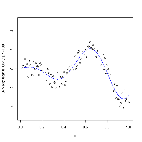
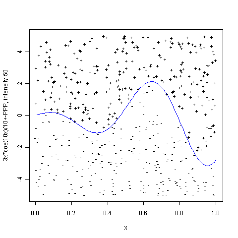
Figure 1. Left: Regression model ${\mathcal{A}}_{n}$ with uniform $U[-1,1]$ errors. Right: Equivalent Poisson point process model ${\mathcal{B}}_{n}$

We may conceive $X_{j}$ as the random point measure $\sum_{k=1}^{N_{j}}\delta_{(x_{k}^{j},y_{k}^{j})}$ where $N_{j}$ is drawn from a Poisson-distribution with intensity $\lVert\lambda_{j}\rVert_{L^{1}(S)}$ and the $(x_{k}^{j},y_{k}^{j})$ are drawn according to the bivariate density $\lambda_{j}/\lVert\lambda_{j}\rVert_{L^{1}(S)}$. The vertical bounds $\pm(C_{\Theta}+1)$ for the domain $S$ are non-informative for $\vartheta\in\Theta$, but the boundedness avoids technicalities. The equivalent unbounded PPP can be described by infinite random point measures $\sum_{k=1}^{\infty}\delta_{(x_{k}^{j},y_{k}^{j})}$ where the $x_{k}^{j}$ are drawn according to the density $f_{D}$ and

$$\textstyle y_{k}^{1}=\vartheta(x_{k}^{1})-(nf_{\varepsilon}(1))^{-1}\sum_{l=1}^{k}z_{l}^{1},\quad y_{k}^{2}=\vartheta(x_{k}^{2})+(nf_{\varepsilon}(-1))^{-1}\sum_{l=1}^{k}z_{l}^{2}$$

holds with exponentially distributed $(z_{k}^{j})$ of mean one (all independent). In this form, the PPP already appears in K01, yielding the limiting law for parametric estimators in the nonregular linear model.

We present the main result of this work in the following theorem.

Theorem 2.1.

The statistical experiments ${\mathcal{A}}_{n}$ and ${\mathcal{B}}_{n}$ are asymptotically equivalent in Le Cam’s sense as $n\to\infty$.

This asymptotic equivalence is achieved constructively by consecutive invertible (in law) and parameter-independent mappings of the data, which generate new experiments where the observation laws are shown to be asymptotically close (uniformly over $\vartheta$ in total variation norm). In order to highlight the main ideas in the subsequent proof and to indicate how to use our theoretical result in practice, let us give an algorithmic description of these equivalence mappings leading from experiment ${\mathcal{A}}_{n}$ to experiment ${\mathcal{B}}_{n}$ (in the version with unbounded domain).

1. Take the data $Y_{j,n}$, $j=1,\ldots,n$, from experiment ${\mathcal{A}}_{n}$.

2. Split the data and bin one part: consider the odd indices $J_{n}:=\{1,3,\ldots,\linebreak 2\lceil n/2\rceil-1\}$ and intervals $I_{k}=[k/m,(k+1)/m)$ with some appropriate $m$. Put ${\bf X}_{1}=(Y_{j+1,n})_{j\in J_{n}\backslash\{n\}}$ and $\bar{\bf Z}=(\bar{Z}_{j})_{j\in J_{n}}$ with

   $$\bar{Z}_{j}=Y_{j,n}-\hat{\vartheta}_{1}(\xi_{j})-\hat{\vartheta}_{1}^{\prime}(\xi_{j})(x_{j}-\xi_{j}),\quad j\in J_{n},$$

   where $\xi_{j}$ is the centre of that interval $I_{k}$ with $x_{j,n}\in I_{k}$ and where $\hat{\vartheta}_{1}$ is a (good) estimator of $\vartheta$ based on the data ${\bf X}_{1}$.

3. Consider the local extremes in $\bar{\bf Z}$, i.e. $s_{k}=\min(\bar{Z}_{k})$, $S_{k}=\max(\bar{Z}_{k})$, $k=0,\ldots,m-1$.

4. Use $\hat{\vartheta}$ on the data ${\bf X}_{1}$ again to transform $s_{k}^{\prime\prime}=s_{k}+\hat{\vartheta}_{1}(\xi_{k})+1$, $S_{k}^{\prime\prime}=S_{k}+\hat{\vartheta}_{1}(\xi_{k})-1$.

5. Randomization to build PPP $X_{l}$, $X_{u}$: on each interval $I_{k}$ generate $(x_{k}^{l},y_{k}^{l})$ with $x_{k}^{l}$ having the density $f_{k}=f_{D}1_{I_{k}}/\int_{I_{k}}f_{D}$ independent of everything else and $y_{k}^{l}=S_{k}^{\prime\prime}-\hat{\vartheta}_{1}^{\prime}(x_{k}^{l})(\xi_{k}-x_{k}^{l})$; define the PPP $X_{l}$ where independently on each $I_{k}$ we observe a point measure in $(x_{k}^{l},y_{k}^{l})$ plus independently (conditionally on $S_{k}^{\prime\prime}$, $\hat{\vartheta}_{1}^{\prime}$) a PPP with intensity

   $$\textstyle\frac{n}{2}f_{\varepsilon}(1)(m\int_{I_{k}}f_{D}){\bf 1}\{x\in I_{k},\,y\leq S_{k}^{\prime\prime}-\hat{\vartheta}_{1}^{\prime}(x)(\xi_{k}-x)\};$$

   analogously generate $x_{k}^{u}$ with the density $f_{k}$ independently, $y_{k}^{u}=s_{k}^{\prime\prime}-\hat{\vartheta}_{1}^{\prime}(x_{k}^{u})(\xi_{k}-x_{k}^{u})$ and use the intensity

   $$\textstyle\frac{n}{2}f_{\varepsilon}(-1)(m\int_{I_{k}}f_{D}){\bf 1}\{x\in I_{k},\,y\geq s_{k}^{\prime\prime}-\hat{\vartheta}_{1}^{\prime}(x)(\xi_{k}-x)\}$$

   to build $X_{u}$ independently conditionally on $s_{k}^{\prime\prime}$, $\hat{\vartheta}_{1}^{\prime}$.

6. Use a (good) estimator $\hat{\vartheta}_{2}$ based on the PPP data ${\bf X}_{2}=(X_{l},X_{u})$ and redo steps (2)-(5) to transform ${\bf X}_{1}$ via $\bar{Z}_{j+1}=Y_{j+1,n}-\hat{\vartheta}_{2}(\xi_{j+1})-\hat{\vartheta}_{2}^{\prime}(\xi_{j+1})(x_{j+1}-\xi_{j+1})$, $j\in J_{n}$, to another couple $(X_{l}^{\prime},X_{u}^{\prime})$ of PPP; the final PPP are obtained by $X_{1}=X_{l}+X_{l}^{\prime}$, $X_{2}=X_{u}+X_{u}^{\prime}$.

In this algorithmic description we could do without substracting and adding the pilot estimator itself (i.e., only use the derivative) in steps (2) and (4), but in the proof this localization permits an easy sufficiency argument for the local extremes. Put in a nutshell, the asymptotic equivalence is achieved by considering block-wise extreme values in the regression experiment, in conjunction with a pre- and post-processing procedure (localization step) performing a linear correction on each block. The easier block-wise constant approximation approach by BL96 does not work here since we need a much higher approximation order.

Throughout we shall write const. for a generic positive constant which may change its value from line to line and does not depend on the parameter $\vartheta$ nor on the sample size $n$. Similarly, the Landau symbols $O$, $o$ and the asymptotic order symbol $\asymp$ will denote uniform bounds with respect to $\vartheta$ and $n$.

3. Pilot estimators

In order to prove Theorem 2.1 a localization strategy is required as in N96 for the density estimation problem. To that end we construct pilot estimators of the target function $\vartheta$ and its derivative in both, experiments ${\mathcal{A}}_{n}$ and ${\mathcal{B}}_{n}$.

Let us fix the estimation point $x_{0}\in[0,1]$ and apply a local polynomial estimation approach. We introduce the neighbourhood $U_{h}=[x_{0}-h,x_{0}+h]$ for $x_{0}\in[h,1-h]$ and the one-sided analogue $U_{h}=[0,2h]$ for $x_{0}\in[0,h)$, $U_{h}=[1-2h,1]$ for $x_{0}\in(1-h,1]$. We introduce the set $\Pi:=\Pi_{2}(U_{h})$ of quadratic polynomials on $U_{h}$. Standard approximation theory (by a Taylor series argument) gives for $h\downarrow 0$

$$\gamma_{h}:=\sup_{\vartheta\in\Theta}\min_{p\in\Pi}\max_{x\in U_{h}}\big{(}h^{-(2+\alpha)}\lvert\vartheta(x)-p(x)\rvert+h^{-(1+\alpha)}\lvert\vartheta^{\prime}(x)-p^{\prime}(x)\rvert\big{)}\leq\text{const.}<\infty\,,$$

where the constant does not depend on $h$.

Definition 3.1.

We call $\hat{\vartheta}\in\Pi$ in experiment ${\mathcal{A}}_{n}$ locally admissible at $x_{0}$ if

$$\max_{j:x_{j,n}\in U_{h}}|Y_{j,n}-\hat{\vartheta}(x_{j,n})|\leq 1+\gamma_{h}h^{2+\alpha}$$

holds. Similarly, in experiment ${\mathcal{B}}_{n}$ we call $\hat{\vartheta}\in\Pi$ locally admissible at $x_{0}$ if

$$X_{1}(\{x\in U_{h},\,y>\hat{\vartheta}(x)+\gamma_{h}h^{2+\alpha}\})=0\text{ and }X_{2}(\{x\in U_{h},\,y<\hat{\vartheta}(x)-\gamma_{h}h^{2+\alpha}\})=0$$

hold. Our estimator $\hat{\vartheta}_{n,h}(x_{0})$ is just any locally admissible $\hat{\vartheta}_{n,h}\in\Pi$, evaluated at $x_{0}$ and selected as a measurable function of the data (by the measurable selection theorem).

Note that the by $\gamma_{h}$ enlarged band size guarantees that $\hat{\vartheta}_{n,h}$ exists since the minimizer $\vartheta_{h}\in\Pi$ in the definition of $\gamma_{h}$ is eligible. The following result gives the pointwise risk bounds for the regression function and its derivative with orders $O(n^{-s/(s+1)})$ and $O(n^{-(s-1)/(s+1)})$, respectively, where $s=2+\alpha$ denotes the regularity in a Hölder class. As an application of our asymptotic equivalence we shall show in Section 8.2 below the optimality of these rates in a minimax sense. The upper bound proof relies on entropy arguments and norm equivalences for polynomials and could be easily extended to more general local polynomial estimation and $L^{p}$-loss functions.

Proposition 3.1.

Select the bandwidth $h$ such that $h\asymp n^{-1/(3+\alpha)}$. Then we have in experiment ${\mathcal{A}}_{n}$ as well as in experiment ${\mathcal{B}}_{n}$

$$\sup_{\vartheta\in\Theta}\sup_{x_{0}\in[0,1]}E_{\vartheta}\big{(}n^{2(2+\alpha)/(3+\alpha)}\big{|}\hat{\vartheta}_{n,h}(x_{0})-\vartheta(x_{0})\big{|}^{2}+n^{2(1+\alpha)/(3+\alpha)}\big{|}\hat{\vartheta}_{n,h}^{\prime}(x_{0})-\vartheta^{\prime}(x_{0})\big{|}^{2}\big{)}\,\leq\,\text{const.}$$

Proof of Proposition 3.1: We shall need the following bounds in $\Pi=\Pi_{2}(U_{h})$ from DL93: $\lVert p\rVert_{L^{\infty}(U_{h})}\leq 8h^{-1}\lVert p\rVert_{L^{1}(U_{h})}$ (their Theorem IV.2.6); $\lVert p^{\prime}\rVert_{L^{\infty}(U_{h})}\leq c_{0}h^{-1}\lVert p\rVert_{L^{\infty}(U_{h})}$ (their Thm. IV.2.7); their proof of Thm. IV.2.6 establishes $\lvert p(x)\rvert\geq(1-4(x-x_{M})/h)\lVert p\rVert_{\infty}$ for $x_{M}:=\text{argmax}_{x\in U_{h}}\lvert p(x)\rvert$ and $x_{M}\leq x<x_{M}+h/4$, assuming without loss of generality that $x_{M}$ lies in the left half of $U_{h}$, such that uniformly over $x_{0}$

$$\lVert p\rVert_{n,h,1}:=\frac{1}{nh}\sum_{x_{j,n}\in U_{h}}\lvert p(x_{j,n})\rvert\geq\text{const.}\cdot\lvert p(x_{M})\rvert=\text{const.}\cdot\lVert p\rVert_{L^{\infty}(U_{h})}$$

is derived.

Let us start with considering the regression experiment ${\mathcal{A}}_{n}$. We apply a standard chaining argument in the finite-dimensional space $\Pi$ together with an approximation argument. From above we have $\lVert p\rVert_{L^{\infty}(U_{h})}/\lVert p\rVert_{n,h,1}\asymp 1$ as well as $\lVert p\rVert_{n,h,1}\geq c_{1}\lvert p(x_{0})\rvert$ with some $c_{1}>0$ uniformly in $p\in\Pi$. Fix $R>2$. For every $\delta>0$ we can find elements $(p_{l})_{l\geq 1}$ that form a $\delta$-net in $\Pi\cap\{\lVert p\rVert_{n,h,1}\geq c_{1}\max(1,c_{0})(R-1)\gamma_{h}h^{2+\alpha}\}$ with respect to the $L^{\infty}(U_{h})$-norm satisfying $\lVert p_{l}\rVert_{n,h,1}\asymp\delta l^{1/3}$ as $l\to\infty$ ; for this note that, by the above norm equivalences, $\Pi\cap\{\lVert p\rVert_{n,h,1}\geq c_{1}\max(1,c_{0})(R-1)\gamma_{h}h^{2+\alpha}\}$ with maximum norm is isometric to ${\mathbb{R}}^{3}\cap\{\lvert x\rvert\geq c_{1}\max(1,c_{0})(R-1)\gamma_{h}h^{2+\alpha}\}$ with the Euclidean metric uniformly for $h\to 0$ and $nh\to\infty$ and use standard coverings of Euclidean balls, e.g. Lemma 2.5 in vdG06. We obtain

$$P_{\vartheta}\Big{(}\exists p\in\Pi:\max_{j:x_{j,n}\in U_{h}}\lvert Y_{j,n}-p(x_{j,n})\rvert\leq 1+\gamma_{h}h^{2+\alpha},\,$$

$$\hskip 85.35826pt\max(h^{-(2+\alpha)}\lvert p(x_{0})-\vartheta(x_{0})\rvert,h^{-(1+\alpha)}\lvert p^{\prime}(x_{0})-\vartheta^{\prime}(x_{0})\rvert)\geq R\gamma_{h}\Big{)}$$

$$=P_{\vartheta}\Big{(}\exists p\in\Pi:\max_{j:x_{j,n}\in U_{h}}\lvert\varepsilon_{j,n}-(p(x_{j,n})-\vartheta(x_{j,n}))\rvert\leq 1+\gamma_{h}h^{2+\alpha},$$

$$\hskip 85.35826pt\,\max(h^{-(2+\alpha)}\lvert p(x_{0})-\vartheta(x_{0})\rvert,h^{-(1+\alpha)}\lvert p^{\prime}(x_{0})-\vartheta^{\prime}(x_{0})\rvert)\geq R\gamma_{h}\Big{)}$$

$$\leq P_{\vartheta}\Big{(}\exists p\in\Pi:\max_{j:x_{j,n}\in U_{h}}\lvert\varepsilon_{j,n}-(p(x_{j,n})-\vartheta_{h}(x_{j,n}))\rvert\leq 1+2\gamma_{h}h^{2+\alpha},\,$$

$$\hskip 85.35826pt\lVert p-\vartheta_{h}\rVert_{n,h,1}\geq\max(1,c_{0})c_{1}(R-1)\gamma_{h}h^{2+\alpha}\Big{)}$$

$$\leq P_{\vartheta}\Big{(}\exists l\geq 1:\max_{j:x_{j,n}\in U_{h}}\lvert\varepsilon_{j,n}-p_{l}(x_{j,n})\rvert\leq 1+2\gamma_{h}h^{2+\alpha}+\delta\Big{)}$$

$$\leq\sum_{l\geq 1}P_{\vartheta}\Big{(}\max_{j:x_{j,n}\in U_{h}}\lvert\varepsilon_{j,n}-p_{l}(x_{j,n})\rvert\leq 1+2\gamma_{h}h^{2+\alpha}+\delta\Big{)}.$$

From $f_{\varepsilon}(-1)>0$, $f_{\varepsilon}(+1)>0$ and the Lipschitz continuity of $f_{\varepsilon}$ within $[-1,1]$ we infer that any $\varepsilon_{j,n}$ satisfies

$$\min\big{(}P(\varepsilon_{j,n}\geq 1-\kappa),P(\varepsilon_{j,n}\leq-1+\kappa)\big{)}\geq c\kappa$$

for some constant $c>0$ and all $\kappa\in(0,1)$. We derive an exponential inequality for any $f:U_{h}\to{\mathbb{R}}$ and $\Delta>0$:

$$P(\max_{j:x_{j,n}\in U_{h}}\lvert\varepsilon_{j,n}-f(x_{j,n})\rvert\leq 1+\Delta)$$

$$\leq\prod_{j:x_{j,n}\in U_{h}}\Big{(}1-\min\Big{(}P(\varepsilon_{j,n}>1+\Delta-\lvert f(x_{j,n})\rvert),\,P(\varepsilon_{j,n}<-1-\Delta+\lvert f(x_{i})\rvert)\Big{)}\Big{)}$$

$$\leq\exp\Big{(}\sum_{j:x_{j,n}\in U_{h}}\log(1-c(\lvert f(x_{i})\rvert-\Delta)_{+})\Big{)}$$

$$\leq\exp\Big{(}-c\sum_{j:x_{j,n}\in U_{h}}(\lvert f(x_{i})\rvert-\Delta)_{+}\Big{)}$$

$$\leq\exp\big{(}-cnh(\lVert f\rVert_{n,h,1}-\Delta)\big{)},$$

using $\log(1+h)\leq h$. We therefore choose $\delta=R\gamma_{h}h^{2+\alpha}$ and arrive at

$$P_{\vartheta}\Big{(}\exists p\in\Pi:p\text{ is locally admissible},\,$$

$$\qquad\max(h^{-(2+\alpha)}\lvert p(x_{0})-\vartheta(x_{0})\rvert,h^{-(1+\alpha)}\lvert p^{\prime}(x_{0})-\vartheta^{\prime}(x_{0})\rvert)\geq R\gamma_{h}\Big{)}$$

$$\leq\sum_{l\geq 1}\exp\Big{(}-\text{const.}\cdot nh(\delta+\gamma_{h}h^{2+\alpha})l^{1/3}\Big{)}=O\Big{(}\exp\Big{(}-\text{const.}\cdot Rnh^{3+\alpha}\Big{)}\Big{)}.$$

We conclude, substituting $h\asymp n^{-1/(3+\alpha)}$, that uniformly over $R\geq 2$

$$P_{\vartheta}\Big{(}h^{-(2+\alpha)}\lvert\hat{\vartheta}_{n,h}(x_{0})-\vartheta(x_{0})\rvert\geq R\gamma_{h}\Big{)} =O(\exp(-\text{const.}\cdot R)),$$

$$P_{\vartheta}\Big{(}h^{-(1+\alpha)}\lvert\hat{\vartheta}_{n,h}^{\prime}(x_{0})-\vartheta^{\prime}(x_{0})\rvert\geq R\gamma_{h}\Big{)} =O(\exp(-\text{const.}\cdot R)).$$

Integrating out these exponential tail bounds yields the desired moment bound in experiment ${\mathcal{A}}_{n}$.

All the results obtained so far remain valid for the PPP experiment ${\mathcal{B}}_{n}$ when the empirical norm $\lVert\cdot\rVert_{n,h,1}$ is replaced by the rescaled $L_{1}(U_{h})$-norm $\lVert g\rVert_{1,U_{h}}:=\frac{1}{h}\int_{U_{h}}\lvert g\rvert$, the admissibility conditions are exchanged and the following (easier) exponential inequality is used:

$$P_{\vartheta}\Big{(}X_{1}(\{x\in U_{h},\,y>\vartheta(x)+f(x)-\Delta\})=0,\,X_{2}(\{x\in U_{h},\,y<\vartheta(x)+f(x)+\Delta\})=0\Big{)}$$

$$=P_{0}\Big{(}X_{1}(\{x\in U_{h},\,y>f(x)-\Delta\})=0\Big{)}P_{0}\Big{(}X_{2}(\{x\in U_{h},\,y<f(x)+\Delta\})=0\Big{)}$$

$$=\exp\Big{(}-nf_{\varepsilon}(1)\int_{U_{h}}(f(x)-\Delta)_{+}f_{D}(x)\,dx\Big{)}$$

$$\hskip 85.35826pt\cdot\exp\Big{(}-nf_{\varepsilon}(-1)\int_{U_{h}}(-f(x)-\Delta)_{+}f_{D}(x)\,dx\Big{)}$$

$$\leq\exp\big{(}-c^{\prime}nh(\lVert f\rVert_{1,U_{h}}-\Delta)\big{)}$$

with some constant $c^{\prime}>0$. $\square$

4. Design adjustment for the regression experiment

We use a piecewise constant approximation strategy and introduce the intervals

$$I_{k,n}=[k/m,(k+1)/m),\quad k=0,\ldots,m-2,\text{ and }I_{m-1,n}=[(m-1)/m,1]$$ (4.1)

for some integer $m$. For any design point $x_{j,n}\in I_{k,n}$ we introduce the centre of the interval

$$\xi_{j,n}:=(k+1/2)/m\text{ for }x_{j,n}\in I_{k,n}.$$ (4.2)

Now we apply a sample splitting scheme and write $J_{n}$ for the collection of odd $j\in\{1,\ldots,n\}$. The experiment ${{\mathcal{A}}_{n}}$ is considered as the totality of the two independent data sets ${\bf X}=(Y_{j+1,n})_{j\in J_{n}}$ and ${\bf Y}^{\prime}=(Y_{j,n})_{j\in J_{n}}$.

Subsequently, we shall not touch upon $\bf X$ to establish asymptotic equivalence, but just assume the existence of sufficiently good estimators based on the data $\bf X$. Therefore, we forget about the specific definition of ${\bf X}$ and write ${\bf X}^{*}$ instead.

Definition 4.1.

Let ${\bf X}^{*}$ be an arbitrary observation in a Polish space, which is independent of ${\bf Y}^{\prime}$. We generalize the experiment ${{\mathcal{A}}_{n}}$ to ${{\mathcal{A}}_{n}}^{*}$, which consists of the data ${\bf Y}^{\prime}$ and ${\bf X}^{*}$.

The original experiment ${{\mathcal{A}}_{n}}$ is still included by putting ${\bf X}^{*}={\bf X}$. This enables us to repeatedly use the following results later also when ${\bf X}^{*}$ will denote a PPP observation.

In a first step we show asymptotic equivalence for the regression experiment ${{\mathcal{A}}_{n}}^{*}$ with the same experiment, but where for $j\in J_{n}$ the regression function is observed at the interval centres $\xi_{j,n}$.

Definition 4.2.

In experiment ${\mathcal{C}}_{n}$ we observe independently the vectors ${\bf X}^{*}$ as under experiment ${{\mathcal{A}}_{n}}^{*}$ and, independently, the vector ${\bf Z}$ with the components

$$Z_{j,n}\,=\,\vartheta(\xi_{j,n})+\varepsilon_{j,n}\,,\qquad j\in J_{n}\,.$$

Lemma 4.1.

Choose $m\in{\mathbb{N}}$ such that $m^{-1}=o(n^{-1/2})$ holds and assume that an estimator $\hat{\vartheta}^{\prime}$ can be constructed based on the data set ${\bf X}^{*}$ with

$$\sup_{\vartheta\in\Theta}\,\sup_{x\in[0,1]}\,E_{\vartheta}|\hat{\vartheta}^{\prime}(x)-\vartheta^{\prime}(x)|\,=\,o(mn^{-1}).$$

Then the experiments ${{\mathcal{A}}_{n}}^{*}$ and ${{\mathcal{C}}_{n}}$ are asymptotically equivalent.

Proof of Lemma 4.1: The observations ${\bf Y}^{\prime}$ from the experiment ${{\mathcal{A}}_{n}}^{*}$ are transformed into the data set $\tilde{{\bf Y}}$ with the components

$$\tilde{Y}_{j,n} \,=\,Y_{j,n}-\hat{\vartheta}^{\prime}(\xi_{j,n})(x_{j,n}-\xi_{j,n})$$

$$\,=\,\vartheta(x_{j,n})-\vartheta^{\prime}(\xi_{j,n})(x_{j,n}-\xi_{j,n})-[\hat{\vartheta}^{\prime}(\xi_{j,n})-\vartheta^{\prime}(\xi_{j,n})](x_{j,n}-\xi_{j,n})+\varepsilon_{j,n}\,,$$

for all $j\in J_{n}$. The data set ${\bf X}^{*}$ is not affected by this transformation. As $\hat{\vartheta}^{\prime}$ is based on the data ${\bf X}^{*}$, this transformation is invertible so that the original data are uniquely reconstructable from the transformed ones; and observing $({\bf X}^{*},{\bf Y}^{\prime})$ on the one hand and $({\bf X}^{*},\tilde{{\bf Y}})$ on the other hand is equivalent. Therefore, for any measurable functional $R$ with $\|R\|_{\infty}\leq 1$ we observe that

$$\big{|}E_{\vartheta}R({\bf X}^{*},\tilde{{\bf Y}})-E_{\vartheta}R({\bf X}^{*},{\bf Z})\big{|} \,\leq\,E_{\vartheta}\big{|}E_{\vartheta}\{R({\bf X}^{*},\tilde{{\bf Y}})|{\bf X}^{*}\}-E_{\vartheta}\{R({\bf X}^{*},{\bf Z})|{\bf X}^{*}\}\big{|}$$ (4.3)

$$\,\leq\,\sum_{j\in J_{n}}E_{\vartheta}\|f_{\tilde{Y}_{j,n}|X^{*}}-f_{Z_{j,n}|X^{*}}\|_{1}\,,$$ (4.4)

where $\|\cdot\|_{1}$ denotes the $L_{1}({\mathbb{R}})$-norm; in general, $f_{Y|X}$ stands for the conditional density of $Y$ given $X$. The conditional independence of the $\tilde{Y}_{j,n}$ and the $Z_{j,n}$ given ${\bf X}^{*}$ as well as an elementary telescopic sum argument with respect to the $L_{1}({\mathbb{R}})$-distance of the multivariate conditional densities of $\tilde{{\bf Y}}$ and ${\bf Z}$ given ${\bf X}^{*}$ have been exploited. We obtain by the Lipschitz continuity of $\varphi$

$$\|f_{\tilde{Y}_{j,n}|X^{*}}-f_{Z_{j,n}|X^{*}}\|_{1}\,\leq\,2\|\varphi\|_{\infty}\cdot|\Delta_{1,j,n}|\,+\,\int_{-1}^{1}|\varphi(x+\Delta_{1,j,n})-\varphi(x)|dx\leq 4C_{\varepsilon}\cdot|\Delta_{1,j,n}|\,,$$ (4.5)

where

$$\Delta_{1,j,n}\,=\,\vartheta(x_{j,n})-\vartheta(\xi_{j,n})-\vartheta^{\prime}(\xi_{j,n})(x_{j,n}-\xi_{j,n})-[\hat{\vartheta}^{\prime}(\xi_{j,n})-\vartheta^{\prime}(\xi_{j,n})](x_{j,n}-\xi_{j,n})\,.$$

We conclude that the total variation distance between $({\bf X}^{*},\tilde{{\bf Y}})$ and $({\bf X}^{*},{\bf Z})$ is bounded from above by

$$\mbox{const.}\cdot\sum_{j\in J_{n}}E_{\vartheta}\big{(}|\Delta_{1,j,n}|\big{)}\,.$$

By the Hölder constraints imposed on the parameter class $\Theta$ we derive that

$$|\Delta_{1,j,n}|\,\leq\,\mbox{const.}\cdot\big{(}m^{-2}+|\hat{\vartheta}^{\prime}(x_{j,n})-\vartheta^{\prime}(x_{j,n})|m^{-1}\big{)}\,.$$

Using $m^{-2}=o(n^{-1})$ and the convergence rate of $\hat{\vartheta}^{\prime}$, we conclude that the Le Cam distance between the experiments ${{\mathcal{A}}_{n}}^{*}$ and ${{\mathcal{C}}_{n}}$ tends to zero uniformly in $\vartheta$, which gives the assertion of the lemma. $\square$

Usually, the bound on the total variation of product measures which is used in the proof is suboptimal, but here the order is optimal due to the singular parts in the measures. Note also that the data $Z_{j,n}$ may be viewed as random responses drawn from a regression function which is locally constant on the intervals $I_{k,n}$ with the values $\vartheta(\xi_{j,n})$ when $x_{j,n}\in I_{k,n}$.

5. Asymptotic equivalence for step functions

We revisit the experiment ${\mathcal{C}}_{n}$ from Definition 4.2. The data $Z_{j,n}$ may be transformed into

$$\tilde{Z}_{j,n}\,=\,Z_{j,n}-\hat{\vartheta}(\xi_{j,n}),$$

where $\hat{\vartheta}$ denotes a preliminary estimator of $\vartheta$ which is based on the data from ${\bf X}^{*}$ as contained in the experiment ${{\mathcal{C}}_{n}}$. Again this transformation is invertible so that the experiment ${\mathcal{C}}_{n}$ is equivalent to the experiment ${{\mathcal{C}}_{n}}^{\prime}$ under which one observes the data ${\bf X}^{*}$ and the vector $\tilde{{\bf Z}}=(\tilde{Z}_{j,n})_{j\in J_{n}}$. The $\tilde{Z}_{j,n}$, $j\in J_{n}$, are conditionally independent given ${\bf X}^{*}$ and have the conditional densities

$$f_{\varepsilon}(x-\Delta_{0,j,n})=\varphi(x-\Delta_{0,j,n})1_{[\Delta_{0,j,n}-1,\Delta_{0,j,n}+1]}(x)\text{ with }\Delta_{0,j,n}=\vartheta(\xi_{j,n})-\hat{\vartheta}(\xi_{j,n}).$$ (5.1)

The next key step is to replace these densities by those with unshifted $\varphi$ where local minima and maxima will turn out to be sufficient statistics.

Definition 5.1.

Let $W_{j,n}$, $j\in J_{n}$, conditionally on ${\bf X}^{*}$ be independent random variables with respective densities

$$f_{W,j}(x) \,=\,\varphi(x)\Big{(}\int_{\Delta_{0,j,n}-1}^{\Delta_{0,j,n}+1}\varphi(t)dt\Big{)}^{-1}1_{[\Delta_{0,j,n}-1,\Delta_{0,j,n}+1]}(x)\,,\qquad j\in J_{n}\,,$$

where $\Delta_{0,j,n}$ is given in (5.1). The experiment in which ${\bf X}^{*}$ and the $W_{j,n}$, $j\in J_{n}$, are observed for $\vartheta\in\Theta$ is denoted by ${\mathcal{D}}_{n}$.

Lemma 5.1.

Suppose that an estimator $\hat{\vartheta}$ of $\vartheta$ can be constructed based on the data set ${\bf X}^{*}$ such that

$$\sup_{\vartheta\in\Theta}\,\sup_{x\in[0,1]}\,E_{\vartheta}|\hat{\vartheta}(x)-\vartheta(x)|^{2}\,=\,O(n^{-1-\delta})\,,$$ (5.2)

for some $\delta>0$. Then the experiments ${\mathcal{C}}_{n}$ and ${\mathcal{D}}_{n}$ are asymptotically equivalent.

Proof of Lemma 5.1: By Le Cam’s inequality and the subadditivity of the squared Hellinger distance $H$ for product measures (cf. Section 2.4 in T09 or Appendix 9.1 in R08) we deduce that for any measurable functional $R$ with $\|R\|_{\infty}\leq 1$ we have

$$|E_{\vartheta}R({\bf X}^{*},\tilde{{\bf Z}})-E_{\vartheta}R({\bf X}^{*},{\bf W})|\, \leq\,E_{\vartheta}\idotsint\Big{|}\prod_{j\in J_{n}}f_{\varepsilon}(y_{j}-\Delta_{0,j,n})-\prod_{j\in J_{n}}f_{W,j}(y_{j})\Big{|}d{\bf y}$$

$$\leq\,2\sum_{j\in J_{n}}E_{\vartheta}H^{2}\big{(}f_{W,j},f_{\varepsilon}(\cdot-\Delta_{0,j,n})\big{)}\,,$$ (5.3)

where the expectation is taken over $\Delta_{0,j,n}$. Hence, it remains to be shown that the sum converges to zero uniformly with respect to $\vartheta\in\Theta$. That sum equals

$$\sum_{j\in J_{n}} E_{\vartheta}\int_{\Delta_{0,j,n}-1}^{\Delta_{0,j,n}+1}\left(\sqrt{\varphi(x)}\Big{(}\int_{\Delta_{0,j,n}-1}^{\Delta_{0,j,n}+1}\varphi(t)dt\Big{)}^{-1/2}-\sqrt{\varphi(x-\Delta_{0,j,n})}\right)^{2}\,dx$$

$$\,\leq\,4C_{\varepsilon}^{2}\,\big{(}2\,+\,\{\inf_{|x|\leq 1}\varphi(x)\}^{-1}\big{)}\,\sum_{j\in J_{n}}E_{\vartheta}\Delta_{0,j,n}^{2}\,,$$

since $\varphi$ is strictly positive, continuous and satisfies the condition (2.4). The imposed convergence rate of the estimator $\hat{\vartheta}$ yields that the supremum taken over $\vartheta\in\Theta$ tends to zero at the rate $O(n^{-\delta})$ and the proof is complete. $\square$

The conditional joint density of the $W_{j,n}$, $j\in J_{n}$, given ${\bf X}^{*}$ from the experiment ${{\mathcal{D}}_{n}}$ can be represented by

$$f_{W}({\bf w})\,=\,\prod_{j\in J_{n}}f_{W,j}(w_{j})\,=\,\Big{(}\prod_{j\in J_{n}}\varphi(w_{j})\Big{)}\Big{(}\prod_{j\in J_{n}}\int_{\Delta_{0,j,n}-1}^{\Delta_{0,j,n}+1}\varphi(t)dt\Big{)}^{-1}$$ (5.4)

$$\cdot\Big{(}\prod_{k=0}^{m-1}1(\min\{w_{j}:x_{j,n}\in I_{k,n}\}\geq\Delta_{0,j(k),n}-1)\cdot 1(\max\{w_{j}:x_{j,n}\in I_{k,n}\}\leq\Delta_{0,j(k),n}+1)\Big{)}\,,$$

where the $I_{k,n}$ are as in Section 4 and $j(k)=\min\{l\in J_{n}:x_{l,n}\in I_{k,n}\}$, ${\bf w}=(w_{j})_{j\in J_{n}}$. Note that the parameter $\vartheta$ is included in the term $\Delta_{0,j(k),n}$.

Definition 5.2.

In experiment ${\mathcal{E}}_{n}$ only the data $({\bf X}^{*},s_{k,n},S_{k,n})$, $k=0,\ldots,m-1$, with

$$s_{k,n} \,=\,\min\{W_{j,n}:x_{j,n}\in I_{k,n}\}\,,$$

$$S_{k,n} \,=\,\max\{W_{j,n}:x_{j,n}\in I_{k,n}\}\,,$$

are observed for $\vartheta\in\Theta$.

An inspection of (5.4) yields that $({\bf X}^{*},s_{k,n},S_{k,n})$, $k=0,\ldots,m-1$, provides a sufficient statistic for the whole empirical information contained in $({\bf X}^{*},\{W_{j,n}:j\in J_{n}\})$ by the Fisher-Neyman factorization theorem.

Sufficiency implies equivalence (e.g. Lemma 3.2 in BL96) and we have

Lemma 5.2.

Experiments ${\mathcal{D}}_{n}$ and ${\mathcal{E}}_{n}$ are equivalent.

In the following we study the conditional distribution of $(s_{k,n},S_{k,n})$ given ${\bf X}^{*}$. Note that, conditionally on ${\bf X}^{*}$, the $(s_{k,n},S_{k,n})$ are independent for $k=0,\ldots,m-1$ as the intervals $I_{k,n}$ are disjoint. We derive that

$$P[s_{k,n}>x,\,S_{k,n}\leq y|{\bf X}^{*}] \,=\,P[W_{j,n}\in(x,y],\,\forall j\in J_{n}\mbox{ with }x_{j,n}\in I_{k,n}|{\bf X}^{*}]$$

$$\,=\,\Big{(}\int_{x}^{y}f_{W,j(k)}(t)dt\Big{)}^{l_{k,n}}\,,$$

for $y>x$. Thus we obtain the conditional joint density of $(s_{k,n},S_{k,n})$ via

$$f_{(s_{k,n},S_{k,n})}(x,y) \,=\,-\frac{\partial^{2}}{\partial x\partial y}P[s_{k,n}>x,\,S_{k,n}\leq y|{\bf X}^{*}]$$

$$\,=\,A_{k,n}(x,y)\cdot l_{k,n}(l_{k,n}-1)f_{W,j(k)}(x)f_{W,j(k)}(y)1_{\{y\geq x\}}\,,$$

where

$$A_{k,n}(x,y) \,=\,\Big{(}1-\int_{\Delta_{0,j(k),n}-1}^{x}f_{W,j(k)}(t)dt-\int_{y}^{\Delta_{0,j(k),n}+1}f_{W,j(k)}(t)dt\Big{)}^{l_{k,n}-2}\,.$$

Definition 5.3.

Consider for each $k$ two conditionally on ${\bf X}^{*}$ independent random variables $s^{\prime}_{k,n}$ and $S^{\prime}_{k,n}$ with conditional exponential densities

$$f_{s^{\prime}_{k,n}}(x) \,=\,(l_{k,n}-2)f_{W,j(k)}(\Delta_{0,j(k),n}-1)\,\exp\big{(}-(l_{k,n}-2)f_{W,j(k)}(\Delta_{0,j(k),n}-1)$$

$$\hskip 142.26378pt\cdot(x-\Delta_{0,j(k),n}+1)\big{)}\,{\bf 1}_{[\Delta_{0,j(k),n}-1,\infty)}(x)\,,$$

$$f_{S^{\prime}_{k,n}}(x) \,=\,(l_{k,n}-2)f_{W,j(k)}(\Delta_{0,j(k),n}+1)\,\exp\big{(}-(l_{k,n}-2)f_{W,j(k)}(\Delta_{0,j(k),n}+1)$$

$$\hskip 142.26378pt\cdot(-x+\Delta_{0,j(k),n}+1)\big{)}\,{\bf 1}_{(-\infty,\Delta_{0,j(k),n}+1]}(x)\,,$$

and the joint density $f_{(s^{\prime}_{k,n},S^{\prime}_{k,n})}$. Then the experiment ${\mathcal{F}}_{n}$ is obtained by observing ${\bf X}^{*}$ as well as conditionally on ${\bf X}^{*}$ independent tuples $(s^{\prime}_{k,n},S^{\prime}_{k,n})$, $k=0,\ldots,m-1$.

Lemma 5.3.

Assume that $m\leq\mbox{const.}\cdot n^{1-\delta}$ for some $\delta>0$ and that

$$\sup_{k=0,\ldots,m-1}|\Delta_{0,j(k),n}|\leq 2C_{\Theta}\,,\qquad\mbox{a.s.}\,,\quad\forall\vartheta\in\Theta\,.$$ (5.5)

Conditionally on the data set ${\bf X}^{*}$, the squared Hellinger distance between $f_{(s^{\prime}_{k,n},S^{\prime}_{k,n})}$ and $f_{(s_{k,n},S_{k,n})}$ satisfies

$$H^{2}(f_{(s^{\prime}_{k,n},S^{\prime}_{k,n})},f_{(s_{k,n},S_{k,n})})\,\leq\,\mbox{const.}\cdot\{\log(n/m)\}^{4}(m/n)^{2}\,,$$

where const. is uniform with respect to $n$, ${\bf X}^{*}$, $\vartheta$ and $k$.

Remark 5.1.

This approximation result together with the ensuing corollary tells us that we need to choose the number $m$ of intervals of polynomially smaller order than $n^{2/3}$. To see that we cannot hope for a better approximation order, note that already in the most simple univariate case where $s:=\min(U_{i},i=1,\ldots,I)$ with $U_{i}$ i.i.d. uniform on $[0,1]$ and $s^{\prime}$ exponentially distributed with intensity $I\in{\mathbb{N}}$, we have for $I\to\infty$

$$H^{2}(f_{s},f_{s^{\prime}}) \geq\int_{0}^{1/I}\big{(}\sqrt{I(1-x)^{I-1}}-\sqrt{I\exp(-Ix)}\big{)}^{2}dx$$

$$\approx\big{(}(1-1/I)^{(I-1)/2}-\exp(-1/2)\big{)}^{2}\asymp I^{-2}.$$

Corollary 5.1.

We assume that an estimator $\hat{\vartheta}$ of $\vartheta$ can be constructed from the data ${\bf X}^{*}$ such that (5.5) holds. For $m=O(n^{2/3-\delta})$ with some $\delta>0$ as $n\to\infty$ the experiments ${\mathcal{E}}_{n}$ and ${\mathcal{F}}_{n}$ are asymptotically equivalent.

Proof of Corollary 5.1: Focussing on the total variation distance between the distributions of the data $\big{(}{\bf X}^{*},\{(s^{\prime}_{k,n},S^{\prime}_{k,n}):k=0,\ldots,m-1\}\big{)}$ and $\big{(}{\bf X}^{*},\{(s_{k,n},S_{k,n}):k=0,\ldots,m-1\}\big{)}$ we consider for any measurable functional $R$ on an appropriate domain and $\|R\|_{\infty}\leq 1$ that

$$\big{|}E_{\vartheta}R({\bf X}^{*},s_{0,n},S_{0,n},\ldots,s_{m-1,n},S_{m-1,n})-E_{\vartheta}R({\bf X}^{*},s^{\prime}_{0,n},S^{\prime}_{0,n},\ldots,s^{\prime}_{m-1,n},S^{\prime}_{m-1,n})\big{|}$$

$$\,\leq\,2\sum_{k=0}^{m-1}E_{\vartheta}H^{2}(f_{(s_{k,n},S_{k,n})},f_{(s^{\prime}_{k,n},S^{\prime}_{k,n})})$$

$$\,\leq\,\mbox{const.}\cdot n^{-\delta/2}\log^{2}n\,,$$

using the conditional independence of the $(s_{k,n},S_{k,n})$, $k=0,\ldots,m-1$, on the one hand and the $(s^{\prime}_{k,n},S^{\prime}_{k,n})$, $k=0,\ldots,m-1$, on the other hand and arguments as in the proof of Lemma 5.1; as well as Lemma 5.3 in the last line. Thus the total variation distance between the distributions of the data $\big{(}{\bf X}^{*},\{(s^{\prime}_{k,n},S^{\prime}_{k,n}):k=0,\ldots,m-1\}\big{)}$ and $\big{(}{\bf X}^{*},\{(s_{k,n},S_{k,n}):k=0,\ldots,m-1\}\big{)}$ converges to zero as $n\to\infty$, which proves the claim of the corollary. $\square$

Proof of Lemma 5.3: First we mention that, although the arguments of the Hellinger distance are most usually densities, its definition $H^{2}(f,g)\,=\,\int(\sqrt{f}(x)-\sqrt{g}(x))^{2}dx$ may easily be extended to all nonnegative functions $f,g\in L_{1}({\mathbb{R}})$. This fact will be used in the sequel. Moreover, note that $l_{k,n}\asymp n/m\geq\text{const.}\cdot n^{\delta}$ holds uniformly over $k$ by our design assumption (2.3). We set

$$f_{1,k,n}(x,y)=\frac{(l_{k,n}-2)^{2}}{l_{k,n}(l_{k,n}-1)}f_{(s_{k,n},S_{k,n})}(x,y)\,,$$

so that

$$H^{2}(f_{1,k,n},f_{(s_{k,n},S_{k,n})})\,\leq\,\frac{(4-3l_{k,n})^{2}}{l_{k,n}(l_{k,n}-1)(l_{k,n}-2)^{2}}\,\asymp\,l_{k,n}^{-2}\,,$$ (5.6)

Note that the support of $f_{(s_{k,n},S_{k,n})}$ and hence of $f_{1,k,n}$ is included in the square $Q_{k,n}=[\Delta_{0,j(k),n}-1,\Delta_{0,j(k),n}+1]^{2}$. A sub-square is defined by

$$Q_{1,k,n}=[\Delta_{0,j(k),n}-1,\Delta_{0,j(k),n}-1+a_{k,n}]\times[\Delta_{0,j(k),n}+1-a_{k,n},\Delta_{0,j(k),n}+1]\subseteq Q_{k,n}\,,$$

which will contain most probability masses, and we set $Q_{2,k,n}=Q_{k,n}\backslash Q_{1,k,n}$ where $a_{k,n}=d_{0}l_{k,n}^{-1}\log l_{k,n}$ with a constant $d_{0}>0$ for $n$ sufficiently large. We split the Hellinger distance into integrals over disjoint domains so that

$$H^{2}(f_{1,k,n},f_{(s^{\prime}_{k,n},S^{\prime}_{k,n})}) \,\leq\,\int_{Q_{1,k,n}}\big{(}\sqrt{f_{1,k,n}}(x,y)-\sqrt{f_{(s^{\prime}_{k,n},S^{\prime}_{k,n})}}(x,y)\big{)}^{2}dx\,dy$$

$$\quad+\,2\int_{Q_{2,k,n}}f_{1,k,n}(x,y)dx\,dy\,+\,2P[s^{\prime}_{k,n}>\Delta_{0,j(k),n}-1+a_{k,n}|{\bf X}^{*}]$$

$$\qquad+\,2P[S^{\prime}_{k,n}<\Delta_{0,j(k),n}+1-a_{k,n}|{\bf X}^{*}]$$

$$=:T_{1}+T_{2}+T_{3}+T_{4}\,.$$ (5.7)

The conditions (2.4) and (5.5) combined with the positivity of $\varphi$ imply that $\|f_{W,j(k)}\|_{\infty}\leq C_{\varepsilon}$ and that

$$\int_{\Delta_{0,j(k),n}-1}^{x}f_{W,j(k)}(t)dt \geq\mbox{const.}\cdot(x-\Delta_{0,j(k),n}+1)\,,\,\forall x\in[\Delta_{0,j(k),n}-1,\Delta_{0,j(k),n}+1],$$

$$\int_{y}^{\Delta_{0,j(k),n}+1}f_{W,j(k)}(t)dt \geq\mbox{const.}\cdot(\Delta_{0,j(k),n}+1-y)\,,\,\forall y\in[\Delta_{0,j(k),n}-1,\Delta_{0,j(k),n}+1].$$

As the Lebesgue measure of $Q_{k,n}$ is equal to $4$, thus bounded, we deduce by the definition of $f_{1,k,n}$ and $f_{(s_{k,n},S_{k,n})}$ that

$$T_{2}\,\leq\,c_{\nu}n^{-\nu}\,,$$

for each $\nu>0$ when selecting the constant $d_{0}$ in the definition of $a_{k,n}$ sufficiently large where $c_{\nu}$ denotes a finite constant which depends on neither the data ${\bf X}^{*}$, $\vartheta$ nor $x,y$.

Concerning terms $T_{3}$ and $T_{4}$, easy calculations yield that these terms are equal to $2\exp\big{\{}-a_{k,n}(l_{k,n}-2)f_{W,j(k)}(\Delta_{0,j(k),n}\mp 1)\big{\}}$, respectively. We may use (2.4), (5.5) and $\varphi>0$ to show that $f_{W,j(k)}(\Delta_{0,j(k),n}\mp 1)\geq\mbox{const}$. Again choosing the constant $d_{0}$ sufficiently large implies that $\max\{T_{3},T_{4}\}\,\leq\,c^{\prime}_{\nu}n^{-\nu}$, for any $\nu>0$ with a constant $c^{\prime}_{\nu}$ which has the same properties as $c_{\nu}$.

Let us focus on the main term $T_{1}$. For $(x,y)\in Q_{1,k,n}$, we have

$$\log A_{k,n}(x,y) \,=\,(l_{k,n}-2)\,\Big{(}-\int_{\Delta_{0,j(k),n}-1}^{x}f_{W,j(k)}(t)dt-\int_{y}^{\Delta_{0,j(k),n}+1}f_{W,j(k)}(t)dt\Big{)}$$

$$\hskip 241.84842pt+R_{1,k,n}(x,y)\,,$$

where $\sup_{(x,y)\in Q_{1,k,n}}\max_{k=0,\ldots,m-1}|R_{1,k,n}(x,y)|\leq\mbox{const.}\cdot l_{k,n}a_{k,n}^{2}\asymp l_{k,n}^{-1}\log^{2}l_{k,n}$ by the Taylor expansion of the logarithm. Furthermore, the functions to be integrated are locally approximated by constant functions,

$$-\int_{\Delta_{0,j(k),n}-1}^{x}f_{W,j(k)}(t)dt-\int_{y}^{\Delta_{0,j(k),n}+1}f_{W,j(k)}(t)dt$$

$$\,=\,-f_{W,j(k)}(\Delta_{0,j(k),n}-1)\cdot(x-\Delta_{0,j(k),n}+1)$$

$$\hskip 128.0374pt-f_{W,j(k)}(\Delta_{0,j(k),n}+1)\cdot(-y+\Delta_{0,j(k),n}+1)+R_{2,k,n}(x,y)\,,$$

where $\sup_{(x,y)\in Q_{1,k,n}}\max_{k=0,\ldots,m-1}|R_{2,k,n}(x,y)|\leq\mbox{const.}\cdot l_{k,n}^{-2}\log^{2}l_{k,n}$, using the Lipschitz continuity of $\varphi$.

We introduce $B_{k,n}(x,y):=A_{k,n}(x,y)f_{W,j(k)}(x)f_{W,j(k)}(y)(l_{k,n}-2)^{2}$ so that $B_{k,n}(x,y)$ coincides with $f_{1,k,n}(x,y)$ on its restriction to $(x,y)\in Q_{1,k,n}$ for $n$ large enough, as well as

$$\tilde{B}_{k,n}(x,y)\,:=\,f_{(s^{\prime}_{k,n},S^{\prime}_{k,n})}(x,y)\frac{f_{W,j(k)}(x)f_{W,j(k)}(y)}{f_{W,j(k)}(\Delta_{0,j(k),n}-1)f_{W,j(k)}(\Delta_{0,j(k),n}+1)}\,.$$

We obtain

$$B_{k,n}^{1/2}(x,y) \,=\,\tilde{B}_{k,n}^{1/2}(x,y)\,\exp\big{(}R_{1,k,n}(x,y)/2+(l_{k,n}-2)R_{2,k,n}(x,y)/2\big{)}$$

$$\,=\,\tilde{B}_{k,n}^{1/2}(x,y)+\tilde{B}_{k,n}^{1/2}(x,y)R_{3,k,n}(x,y)\,,$$

where $\sup_{(x,y)\in Q_{1,k,n}}\max_{k=0,\ldots,m-1}|R_{3,k,n}(x,y)|\leq\mbox{const.}\cdot l_{k,n}^{-1}\log^{2}l_{k,n}$ so that

$$\tilde{B}_{k,n}^{1/2}(x,y)\,=\,f_{(s^{\prime}_{k,n},S^{\prime}_{k,n})}^{1/2}(x,y)+f_{(s^{\prime}_{k,n},S^{\prime}_{k,n})}^{1/2}(x,y)R_{4,k,n}(x,y)\,,$$

where

$$|R_{4,k,n}(x,y)| \,\leq\,\mbox{const.}\cdot\big{(}|f_{W,j(k)}(x)-f_{W,j(k)}(\Delta_{0,j(k),n}-1)|$$

$$\hskip 113.81102pt+|f_{W,j(k)}(y)-f_{W,j(k)}(\Delta_{0,j(k),n}+1)|\big{)}$$

$$\,\leq\,\mbox{const.}\cdot a_{k,n}\,\asymp\,l_{k,n}^{-1}\log l_{k,n}\,,$$

where the conditions (5.5), (2.4) and their consequences have been used. We conclude that

$$B_{k,n}^{1/2}(x,y) \,=\,f_{(s^{\prime}_{k,n},S^{\prime}_{k,n})}^{1/2}(x,y)+f_{(s^{\prime}_{k,n},S^{\prime}_{k,n})}^{1/2}(x,y)R_{5,k,n}(x,y)\,,$$

where $\sup_{(x,y)\in Q_{1,k,n}}\max_{k=0,\ldots,m-1}|R_{5,k,n}(x,y)|\leq\mbox{const.}\cdot l_{k,n}^{-1}\log^{2}l_{k,n}$. Hence, the term $T_{1}$ is bounded from above by

$$T_{1} \,\leq\,\int_{Q_{1,k,n}}R_{5,k,n}^{2}(x,y)f_{(s^{\prime}_{k,n},S^{\prime}_{k,n})}(x,y)\,dx\,dy\,\leq\,\mbox{const.}\cdot(\log^{4}l_{k,n})l_{k,n}^{-2}\,,$$

as the density $f_{(s^{\prime}_{k,n},S^{\prime}_{k,n})}$ integrates to one. By inserting the upper bounds on $T_{1},\ldots,T_{4}$ into (5.7) and combining that result with (5.6), we complete the proof. $\square$

Definition 5.4.

In experiment ${\mathcal{G}}_{n}$ we observe the data $({\bf X}^{*},(d_{k,n},D_{k,n})_{k=0,\ldots,m-1})$ for $\vartheta\in\Theta$ where $d_{0,n},D_{0,n},\ldots,d_{m-1,n},D_{m-1,n}$ are independent random variables, also independent of ${\bf X}^{*}$, with densities

$$f_{d_{k,n}}(x) \,=\,\rho_{k,n}\varphi(-1)\,\exp\big{(}-\rho_{k,n}\varphi(-1)\cdot[x-\vartheta(\xi_{j(k),n})]\big{)}\,{\bf 1}_{[\vartheta(\xi_{j(k),n}),\infty)}(x)\,,$$

$$f_{D_{k,n}}(x) \,=\,\rho_{k,n}\varphi(1)\,\exp\big{(}\rho_{k,n}\varphi(1)\cdot[x-\vartheta(\xi_{j(k),n})]\big{)}\,{\bf 1}_{(-\infty,\vartheta(\xi_{j(k),n})]}(x)\,,$$

where $\rho_{k,n}=(n/2)\int_{I_{k,n}}f_{D}(t)dt$ with $f_{D}$ as in (2.2).

Lemma 5.4.

We select $m$ such that $m=o(n^{2/3})$. Also we assume the existence of an estimator $\hat{\vartheta}$ of $\vartheta$ based on ${\bf X}^{*}$ such that (5.5) and

$$\sup_{\vartheta\in\Theta}\,\sup_{x\in[0,1]}\,E_{\vartheta}|\hat{\vartheta}(x)-\vartheta(x)|^{2}\,=\,o(m^{-1})$$

are fulfilled. Then the experiments ${\mathcal{F}}_{n}$ and ${\mathcal{G}}_{n}$ are asymptotically equivalent as $n\to\infty$.

Proof of Lemma 5.4: As the estimator $\hat{\vartheta}$ is based on the data set ${\bf X}^{*}$ the transformation ${\mathcal{T}}$ which maps the observations $\big{(}{\bf X}^{*},\{(s^{\prime}_{k,n},S^{\prime}_{k,n}):k=0,\ldots,m-1\}\big{)}$ to $\big{(}{\bf X}^{*},\{(s^{\prime\prime}_{k,n},S^{\prime\prime}_{k,n}):k=0,\ldots,m-1\}\big{)}$ with $s^{\prime\prime}_{k,n}=s^{\prime}_{k,n}+\hat{\vartheta}(\xi_{j(k),n})+1$ and $S^{\prime\prime}_{k,n}=S^{\prime}_{k,n}+\hat{\vartheta}(\xi_{j(k),n})-1$ is invertible. Therefore, the experiment under which the data $\big{(}{\bf X}^{*},\{(s^{\prime\prime}_{k,n},S^{\prime\prime}_{k,n}):k=0,\ldots,m-1\}\big{)}$ are observed is equivalent to the experiment ${\mathcal{F}}_{n}$.

The squared Hellinger distance between the exponential densities with the same endpoint and the scaling parameters $\mu_{1}$ and $\mu_{2}$ turns out to be $2(\mu_{1}-\mu_{2})^{2}(\mu_{1}+\mu_{2})^{-1}(\sqrt{\mu_{1}}+\sqrt{\mu_{2}})^{-2}$.

Also, (2.2) implies that $|l_{k,n}-\rho_{k,n}|\leq 2$ for all $k=0,\ldots,m-1$. We may set $\mu_{1,\pm}=\rho_{k,n}\varphi(\pm 1)\int_{\Delta_{0,j(k),n}-1}^{\Delta_{0,j(k),n}+1}\varphi(t)dt$ and $\mu_{2,\pm}=(l_{k,n}-2)\varphi(\Delta_{0,j(k),n}\pm 1)$. Hence,

$$H^{2}(f_{S^{\prime\prime}_{k,n}},f_{D_{k,n}})+H^{2}(f_{s^{\prime\prime}_{k,n}},f_{d_{k,n}})\,\leq\,\mbox{const.}\cdot\{l_{k,n}^{-2}+\Delta_{0,j(k),n}^{2}\}\,,$$

where the constant does not depend on ${\bf X}^{*}$. Therein we have utilized condition (5.5) as well as the Lipschitz continuity, positivity and boundedness of $\varphi$. We take the expectation of the sum of these terms over $k=0,\ldots,m-1$ which converges to zero uniformly in $\vartheta\in\Theta$ by the assumption on $m$ and the imposed convergence rates of the estimator $\hat{\vartheta}$. Then the asymptotic equivalence is evident by the argument (5.3) from the proof of Lemma 5.1 when replacing the data sets $\tilde{Z}$ and ${\bf W}$ by the data samples $(d_{k,n},D_{k,n})_{k=0,\ldots,m-1}$ and $(s^{\prime\prime}_{k,n},S^{\prime\prime}_{k,n})_{k=0,\ldots,m-1}$, respectively, and inserting the conditional densities of their components given ${\bf X}^{*}$. The sum is, of course, to be taken over $k=0,\ldots,m-1$ instead of $j\in J_{n}$. $\square$

Now we go over to experiments involving Poisson point processes (PPP).

Definition 5.5.

In experiment ${\mathcal{H}}_{n}$ we observe ${\bf X}^{*}$ and independently two independent Poisson point processes $X_{l}$ and $X_{u}$ whose domain is the Borel $\sigma$-algebra of ${\mathbb{R}}^{2}$ and whose intensity functions equal

$$\lambda_{l}(x,y) \,=\,m\varphi(1)\sum_{k=0}^{m-1}\rho_{k,n}{\bf 1}_{I_{k,n}}(x){\bf 1}_{[-C_{\Theta}-1,\vartheta(\xi_{j(k),n})]}(y)\,,$$

$$\lambda_{u}(x,y) \,=\,m\varphi(-1)\sum_{k=0}^{m-1}\rho_{k,n}{\bf 1}_{I_{k,n}}(x){\bf 1}_{[\vartheta(\xi_{j(k),n}),C_{\Theta}+1]}(y)\,,$$

and are hence locally constant. We recall that $C_{\Theta}$ is the uniform upper bound on $|\vartheta|$ in the parameter set $\Theta$.

We define the extreme points of $X_{l}$ and $X_{u}$ in the strip $I_{k,n}\times{\mathbb{R}}$ by

$$X_{l,k} \,=\,\inf\big{\{}y\in{\mathbb{R}}\,:\,X_{l}(I_{k,n}\times[y,\infty))=0\big{\}}\,,$$

$$X_{u,k} \,=\,\sup\big{\{}y\in{\mathbb{R}}\,:\,X_{u}(I_{k,n}\times(-\infty,y])=0\big{\}}\,.$$

Lemma 5.5.

(a)  The statistic $(X_{l,k},X_{u,k})$, $k=0,\ldots,m-1$, is sufficient for the whole empirical information contained in $X_{l}$ and $X_{u}$.
(b)  The distribution functions of $X_{l,k}$ and $X_{u,k}$ are equal to those of $\max\{-C_{\Theta}-1,D_{k,n}\}$ and $\min\{C_{\Theta}+1,d_{k,n}\}$, respectively where $d_{k,n}$ and $D_{k,n}$ are as in experiment ${\mathcal{G}}_{n}$. Moreover, all $X_{l,k}$, $k=0,\ldots,m-1$, on the one hand and all $X_{u,k}$, $k=0,\ldots,m-1$ on the other hand are independent.

Proof of Lemma 5.5: (a)  Let $X_{0}$ denote the PPP with the intensity function $\lambda_{0}={\bf 1}_{[0,1]\times[-C_{\Theta}-1,C_{\Theta}+1]}$. The probability measures generated by $X_{0},X_{l},X_{u}$ are denoted by ${\bf P}_{0},{\bf P}_{l},{\bf P}_{u}$, respectively. As the functions $\lambda_{0},\lambda_{l},\lambda_{u}$ are piecewise constant and the support of $\lambda_{l}$ and $\lambda_{u}$ is included in that of $\lambda_{0}$ the measure ${\bf P}_{0}$ dominates ${\bf P}_{l}$ and ${\bf P}_{u}$ and the corresponding Radon-Nikodym derivatives are equal to

$$\frac{d{\bf P}_{l}}{d{\bf P}_{0}}(X) \,=\,\exp\Big{\{}\int\log\frac{\lambda_{l}(x,y)}{\lambda_{0}(x,y)}dX(x,y)-\int\Big{(}\frac{\lambda_{l}(x,y)}{\lambda_{0}(x,y)}-1\Big{)}\lambda_{0}(x,y)\,dx\,dy\Big{\}}\,,$$

$$\frac{d{\bf P}_{u}}{d{\bf P}_{0}}(X) \,=\,\exp\Big{\{}\int\log\frac{\lambda_{u}(x,y)}{\lambda_{0}(x,y)}dX(x,y)-\int\Big{(}\frac{\lambda_{u}(x,y)}{\lambda_{0}(x,y)}-1\Big{)}\lambda_{0}(x,y)\,dx\,dy\Big{\}}\,,$$

see e.g. Theorem 1.3 in K98 which apparently goes back to B71. Therein $X$ may be viewed as an arbitrary counting process on the Borel $\sigma$-algebra of $[0,1]\times[-C_{\Theta}-1,C_{\Theta}+1]$. We write $\Gamma_{\vartheta}=\bigcup_{k=0}^{m-1}I_{k,n}\times(\vartheta(\xi_{j(k),n}),C_{\Theta}+1]$ and $\Phi=\bigcup_{k=0}^{m-1}I_{k,n}\times[-C_{\Theta}-1,\tilde{X}_{l,k}]$ where $\tilde{X}_{l,k}$ equals $X_{l,k}$ except that $X_{l}$ is changed into the general process $X$ in the definition. Then $d{\bf P}_{l}/d{\bf P}_{0}$ is equal to

$$\frac{d{\bf P}_{l}}{d{\bf P}_{0}}(X) \,=\,{\bf 1}_{\{\emptyset\}}(\Gamma_{\vartheta}\cap\Phi)\cdot\exp\Big{\{}\sum_{k=0}^{m-1}\log[\rho_{k,n}m\varphi(1)]X(I_{k,n}\times[-C_{\Theta}-1,C_{\Theta}+1])\Big{\}}$$

$$\hskip 56.9055pt\cdot\exp\Big{\{}-\sum_{k=0}^{m-1}(\vartheta(\xi_{j(k),n})+C_{\Theta}+1)\rho_{k,n}\varphi(1)\Big{\}}\exp(2C_{\Theta}+2)\,,$$

where we have used that $X(I_{k,n}\times[-C_{\Theta}-1,C_{\Theta}+1])=X(I_{k,n}\times[-C_{\Theta}-1,\vartheta(\xi_{j(k),n})])$ whenever $X(\Gamma_{\vartheta})=0$; and that $\Gamma_{\vartheta}$ and $\Phi$ are disjoint if and only if $X(\Gamma_{\vartheta})=0$. It follows from the Fisher-Neyman factorization theorem that the $X_{l,k}$, $k=0,\ldots,m-1$ represent a sufficient statistic for $X_{l}$. The corresponding assertion for the $X_{u,r}$ is proved analogously.

(b)  We consider for $x\in[-C_{\Theta}-1,\vartheta(\xi_{j(k),n})]$ that

$$P[X_{l,k}\leq x] \,=\,P[X_{l}(I_{k,n}\times(x,\infty))=0]\,=\,\exp\big{(}-(\vartheta(\xi_{j(k),n})-x)\rho_{k,n}\varphi(1)\big{)}$$

$$\,=\,P[D_{k,n}\leq x]\,.$$

Clearly we have $P[X_{l,k}>\vartheta(\xi_{j(k),n})]=P[D_{k,n}>\vartheta(\xi_{j(k),n})]=0$ and $P[X_{l,k}<-C_{\Theta}-1]=0$ so that the distribution functions of $X_{l,k}$ and $\max\{-C_{\Theta}-1,D_{k,n}\}$ coincide. The claim that $X_{u,k}$ and $\min\{C_{\Theta}+1,d_{k,n}\}$ are identically distributed follows analogously. Finally the independence of the data $X_{l,k}$, $k=0,\ldots,m-1$ as well as of the data $X_{u,k}$, $k=0,\ldots,m-1$ follows from the fact that $X(A_{0}),\ldots,X(A_{m-1})$ are independent for all $A_{k}\subseteq I_{k,n}\times[-C_{\Theta}-1,C_{\Theta}+1]$ by the definition of the PPP. $\square$

Lemma 5.6.

For $m=O(n^{1-\delta})$, $\delta>0$, the total variation distance between the distributions of $\big{(}(\min\{C_{\Theta}+1,d_{k,n}\},\max\{-C_{\Theta}-1,D_{k,n}\}):k=0,\ldots,m-1\big{)}$ and $\big{(}(d_{k,n},D_{k,n}):k=0,\ldots,m-1\big{)}$ converges to zero.

Proof of Lemma 5.6: Due to the independence of the data the desired total variation distance is bounded from above by the sum of the total variation distances between the distributions of $d_{k,n}$ and $\min\{C_{\Theta}+1,d_{k,n}\}$ plus the corresponding distances between the distributions of $D_{k,n}$ and $\max\{-C_{\Theta}-1,D_{k,n}\}$ where $k=0,\ldots,m-1$. The total variation distance between $d_{k,n}$ and $\min\{C_{\Theta}+1,d_{k,n}\}$ is bounded by

$$2P[d_{k,n}\geq C_{\Theta}+1]\,\leq\,2\exp\big{(}-\mbox{const.}\cdot n/m\big{)}\,,$$

so that because of $m\leq\mbox{const.}\cdot n^{1-\delta}$ the sum of these terms for $k=0,\ldots,m-1$ tends to zero exponentially fast. The distributions of $\max\{-C_{\Theta}-1,D_{k,n}\}$ and $D_{k,n}$ are treated in the same way. $\square$.

Combining these two lemmata we obtain directly asymptotic equivalence.

Corollary 5.2.

Experiments ${\mathcal{G}}_{n}$ and ${\mathcal{H}}_{n}$ are asymptotically equivalent for $m$ as in Lemma 5.6.

We observe that the choice $m\asymp n^{2/3-\delta}$ for some $\delta\in(0,1/6)$ meets all requirements imposed on $m$ so far and we summarize our results.

Proposition 5.1.

Select $m\asymp n^{2/3-\delta}$ for some $\delta\in(0,1/6)$ and suppose that there is an estimator $\hat{\vartheta}$, based on the data ${\bf X}^{*}$ alone, which satisfies (5.5) and

$$\sup_{\vartheta\in\Theta}\,\sup_{x\in[0,1]}\,E_{\vartheta}|\hat{\vartheta}(x)-\vartheta(x)|^{2}\,=\,O(n^{-1-\delta}).$$

Then we have asymptotic equivalence between experiments ${\mathcal{C}}_{n}$ and ${\mathcal{H}}_{n}$. Moreover, if we have additionally

$$\sup_{\vartheta\in\Theta}\,\sup_{x\in[0,1]}\,E_{\vartheta}|\hat{\vartheta}^{\prime}(x)-\vartheta^{\prime}(x)|\,=\,o(n^{-1/3-\delta}),$$

then also ${{\mathcal{A}}_{n}}^{*}$ and ${\mathcal{H}}_{n}$ are asymptotically equivalent.

6. Localization of the PPP model

The processes $X_{l}$ and $X_{u}$ in the experiment ${\mathcal{H}}_{n}$ have step functions as their intensity boundaries which approximate continuous functions as $m$ tends to infinity. Therefore we consider now the experiment where ${\bf X}^{*}$ and independently two PPP with boundary function $\vartheta$ are observed.

Definition 6.1.

In experiment ${\mathcal{I}}_{n}$ we observe ${\bf X}^{*}$ and independently two independent PPP $X_{1,0}$ and $X_{2,0}$ with intensities

$$\lambda_{1,0}(x,y) \,=\,(n/2)f_{\varepsilon}(1)f_{D}(x){\bf 1}_{[-C_{\Theta}-1,\vartheta(x)]}(y)\,,$$

$$\lambda_{2,0}(x,y) \,=\,(n/2)f_{\varepsilon}(-1)f_{D}(x){\bf 1}_{[\vartheta(x),C_{\Theta}+1]}(y)\,.$$ (6.1)

Proposition 6.1.

We impose the conditions of Lemma 4.1 and, in addition, that for all $\vartheta\in\Theta$, we have

$$\sup_{x\in[0,1]}|\hat{\vartheta}^{\prime}(x)|\,\leq\,2\sup_{\vartheta\in\Theta}\sup_{x\in[0,1]}|\hat{\vartheta}^{\prime}(x)|\,,\qquad\mbox{a.s.}$$ (6.2)

Then the experiments ${\mathcal{H}}_{n}$ and ${\mathcal{I}}_{n}$ are asymptotically equivalent.

Proof of Proposition 6.1: First, we show asymptotic equivalence of the experiment ${\mathcal{H}}_{n}$ with the experiment ${{\mathcal{H}}_{n}}^{\prime}$ in which one observes the data $({\bf X}^{*},\tilde{X}_{1},\tilde{X}_{2})$ where $\tilde{X}_{1}$ and $\tilde{X}_{2}$ are PPP with the intensity functions

$$\tilde{\lambda}_{1}(x,y) \,=\,(n/2)f_{\varepsilon}(1)f_{D}(x){\bf 1}_{[-C_{\Theta}-1,\vartheta(x)-\hat{\vartheta}^{\prime}(x)(\xi(x)-x)]}(y)\,,$$

$$\tilde{\lambda}_{2}(x,y) \,=\,(n/2)f_{\varepsilon}(-1)f_{D}(x){\bf 1}_{[\vartheta(x)-\hat{\vartheta}^{\prime}(x)(\xi(x)-x),C_{\Theta}+1]}(y)\,,$$

conditionally on ${\bf X}^{*}$, respectively. Here, $\hat{\vartheta}^{\prime}$ denotes the pilot estimator from Lemma 4.1 based on the data set ${\bf X}^{*}$; and we write $\xi(x)$ for the centre of that interval $I_{k,n}$ which contains the element $x$.

By a similar argument as in (4.3), it suffices to show that the expected Hellinger distance between the distribution of $\tilde{X}_{1}$ and $X_{l}$ on the one hand and $\tilde{X}_{2}$ and $X_{u}$ on the other hand converges to zero. We shall now employ a general formula bounding the Hellinger distance between two PPP laws $P_{1},P_{2}$ with respective intensities $\lambda_{1},\lambda_{2}$ by the (generalized) Hellinger distance of the intensities ; when $P$ denotes the law of the PPP with intensity $\lambda=\lambda_{1}+\lambda_{2}$, we derive from the likelihood expression

$$H^{2} (P_{1},P_{2})=2\Big{(}1-E_{\vartheta}\exp\Big{(}\int\frac{1}{2}(\log(\lambda_{1}/\lambda)+\log(\lambda_{2}/\lambda))dX-\int\Big{(}\frac{\lambda_{1}+\lambda_{2}}{2\lambda}-1\Big{)}\lambda\Big{)}\Big{)}$$

$$=2\Big{(}1-\Big{\{}E_{\vartheta}\exp\Big{(}\int\log\sqrt{\lambda_{1}\lambda_{2}}/\lambda\,dX-\int(\sqrt{\lambda_{1}\lambda_{2}}/\lambda-1)\lambda\Big{)}\Big{\}}$$

$$\hskip 256.0748pt\cdot\exp\Big{(}-\int(\sqrt{\lambda_{1}}-\sqrt{\lambda_{2}})^{2}/2\Big{)}\Big{)}$$

$$=2\left(1-\exp\left(-\int(\sqrt{\lambda_{1}}-\sqrt{\lambda_{2}})^{2}/2\right)\right)$$ (6.3)

$$\leq\int(\sqrt{\lambda_{1}}-\sqrt{\lambda_{2}})^{2}\,,$$

where we have used the fact that the Radon-Nikodym-derivative of the PPP-law with intensity $\sqrt{\lambda_{1}\lambda_{2}}$ with respect to $P$ integrates to one under $P$, see also LCY00 for a related result. Thus we bound the Hellinger distance between the intensities of $\tilde{X}_{1}$ and $X_{l}$ by

$$\int(\sqrt{\lambda_{l}}-\sqrt{\tilde{\lambda}_{1}})^{2}\,\leq\,\mbox{const.}\cdot n\,\sum_{k=0}^{m-1}\Big{\{}\int_{I_{k,n}} \big{|}\vartheta(\xi(x))-\vartheta(x)+\hat{\vartheta}^{\prime}(x)(\xi(x)-x)\big{|}dx$$

$$\,+\,\int_{I_{k,n}}\Big{|}f_{D}(x)-m\int_{I_{k,m}}f_{D}(y)dy\Big{|}^{2}dx\Big{\}}\,,$$

where the constant does not depend on ${\bf X}^{*}$. As $f_{D}$ is assumed to be Lipschitz on $[0,1]$ the latter term contributes to the asymptotic order by the deterministic upper bound $O\big{(}nm^{-2}\big{)}$ independently of $\vartheta$. Then we apply the expectation to the above expression and we obtain

$$O\big{(}nm^{-2}\big{)}+\mbox{const.}\cdot nm^{-1}\sup_{\vartheta\in\Theta}\sup_{x\in[0,1]}E_{\vartheta}\big{|}\hat{\vartheta}^{\prime}(x)-\vartheta^{\prime}(x)\big{|}=o(1)\,,$$

as a uniform upper bound. Together with the same bound for the Hellinger distance, conditionally on ${\bf X}^{*}$, between the intensities of $\tilde{X}_{2}$ and $X_{u}$ this implies asymptotic equivalence between ${\mathcal{H}}_{n}$ and ${{\mathcal{H}}_{n}}^{\prime}$ again by arguments as in (5.3).

For any two-dimensional Borel set $B$ let us define the pointwise shifted version

$$\hat{B}\,=\,\big{\{}(x,y)\in{\mathbb{R}}^{2}\,:\,\big{(}x,y+\hat{\vartheta}^{\prime}(x)[\xi(x)-x]\big{)}\in B\big{\}}\,,$$

and the processes $\overline{X}_{j}(B)\,=\,\tilde{X}_{j}(\hat{B})$, $j=1,2$, conditionally on the data set ${\bf X}^{*}$. Note that $\hat{B}$ is a Borel set as well whenever the shift function $\hat{\vartheta}^{\prime}(\cdot)[\xi(\cdot)-\cdot]$ is piecewise continuous on the intervals $I_{k,n}$. Then $\overline{X}_{j}$ represents a PPP with the shifted intensity function

$$\overline{\lambda}_{1}(x,y) \,=\,(n/2)\varphi(1)f_{D}(x){\bf 1}_{[-C_{\Theta}-1+\hat{\vartheta}^{\prime}(x)(\xi(x)-x),\vartheta(x)]}(y)$$

$$\overline{\lambda}_{2}(x,y) \,=\,(n/2)\varphi(-1)f_{D}(x){\bf 1}_{[\vartheta(x),C_{\Theta}+1+\hat{\vartheta}^{\prime}(x)(\xi(x)-x)]}(y)\,.$$

Note that this transformation is invertible as long as the data set ${\bf X}^{*}$ is available. Therefore, the experiment ${{\mathcal{H}}_{n}}^{\prime\prime}$ of observing ${\bf X}^{*}$ and $\overline{X}_{j}$, $j=1,2$ independently is equivalent to the experiment ${{\mathcal{H}}_{n}}^{\prime}$.

By the imposed upper bound on the estimator $\hat{\vartheta}^{\prime}$ we may assume that

$$\sup_{\vartheta\in\Theta}\sup_{x\in[0,1]}|\hat{\vartheta}^{\prime}(x)||\xi(x)-x|\,\leq\,1/2\,,$$

for $m$ sufficiently large. Hence, the observation of $\overline{X}_{j}$, $j=1,2$, is equivalent with the observation of two conditionally independent Poisson processes $\overline{X}_{j,1}$ and $\overline{X}_{j,2}$ with the intensity functions

$$\overline{\lambda}_{1,1}(x,y) \,=\,(n/2)\varphi(1)f_{D}(x){\bf 1}_{[-C_{\Theta}-1/2,\vartheta(x)]}(y)\,,$$

$$\overline{\lambda}_{1,2}(x,y) \,=\,(n/2)\varphi(1)f_{D}(x){\bf 1}_{[-C_{\Theta}-1+\hat{\vartheta}^{\prime}(x)(\xi(x)-x),-C_{\Theta}-1/2)}(y)\,,$$

$$\overline{\lambda}_{2,1}(x,y) \,=\,(n/2)\varphi(-1)f_{D}(x){\bf 1}_{[\vartheta(x),C_{\Theta}+1/2]}(y)\,,$$

$$\overline{\lambda}_{2,2}(x,y) \,=\,(n/2)\varphi(-1)f_{D}(x){\bf 1}_{(C_{\Theta}+1/2,C_{\Theta}+1+\hat{\vartheta}^{\prime}(x)(\xi(x)-x)]}(y)\,,$$

Thus all processes $\overline{X}_{j,i}$, $i,j=1,2$, are independent. Also we realize that the processes $\overline{X}_{1,2}$ and $\overline{X}_{2,2}$ represent conditionally ancillary statistics given the data set ${\bf X}^{*}$ as $\overline{\lambda}_{1,2}$ and $\overline{\lambda}_{2,2}$ do not explicitly depend on $\vartheta$, but are fixed by knowledge of ${\bf X}^{*}$ for $n$ sufficiently large. Therefore, the observation of ${\bf X}^{*}$ and $\overline{X}_{j,1}$, $j=1,2$ is sufficient for complete empirical information contained in experiment ${{\mathcal{H}}_{n}}^{\prime\prime}$. On the other hand we may also add two independent PPP $\overline{X}_{j,3}$, $j=1,2$ with the intensity functions

$$\overline{\lambda}_{1,3}(x,y) \,=\,(n/2)\varphi(1)f_{D}(x){\bf 1}_{[-C_{\Theta}-1,-C_{\Theta}-1/2)}(y)\,,$$

$$\overline{\lambda}_{2,3}(x,y) \,=\,(n/2)\varphi(-1)f_{D}(x){\bf 1}_{(C_{\Theta}+1/2,C_{\Theta}+1]}(y)\,,$$

which are totally uninformative. Combining the independent processes $\overline{X}_{j,1}$ and $\overline{X}_{j,3}$ whose intensity functions are supported on (almost) disjoint domains for both $j=1,2$, the considered experiment is equivalent to the experiment ${{\mathcal{I}}_{n}}$. $\square$

7. Final proof

In this section, we combine all results derived in the previous sections in order to complete the proof of Theorem 2.1. For simplicity we suppose that $n$ is even. By Proposition 3.1 with sample size $n/2$, there exists an estimator $\hat{\vartheta}$ based on the data ${\bf X}={\bf X}^{*}$ from experiment ${{\mathcal{A}}_{n}}$ which satisfies the conditions of Proposition 5.1, e.g. by choosing $\delta=\alpha/2$. Therefore, experiments ${\mathcal{A}}_{n}$ and ${\mathcal{I}}_{n}$ are asymptotically equivalent by Propositions 5.1 and 6.1. The conditions (5.5) and (6.2) are satisfied when truncating the range of $\hat{\vartheta}$ and $\hat{\vartheta}^{\prime}$ suitably without losing validity of Proposition 3.1. Therein, note that the uniform upper bounds on $\vartheta\in\Theta$ as well as on its derivative are known. Then we set ${{\mathcal{A}}_{n}}^{*}={\mathcal{I}}_{n}$ by using the processes $X_{1,0}$ and $X_{2,0}$ as the data set ${\bf X}^{*}$ and let ${\bf X}$ take the role of the data ${\bf Y}^{\prime}$ from experiment ${{\mathcal{A}}_{n}}$. Note that all of our arguments from the previous sections remain valid when transforming the responses with even instead of odd observation number. Applying Propositions 5.1 and 6.1 again, we obtain asymptotic equivalence of the experiments ${{\mathcal{I}}_{n}}$ and ${{\mathcal{J}}_{n}}$ where the latter model just consists of $X_{1,0}$ and $X_{2,0}$ and two independent copies $X_{1,0}^{*}$ and $X_{2,0}^{*}$. The likelihood process of experiment ${\mathcal{J}}_{n}$ and experiment ${\mathcal{B}}_{n}$ turns out to be the same, using Theorem 1.3 in K98 as in the proof of Lemma 5.5, such that ${\mathcal{J}}_{n}$ and ${\mathcal{B}}_{n}$ are equivalent experiments. The concrete equivalence mapping is given by looking at the sum of the processes $X_{j}=X_{j,0}+X_{j,0}^{\ast}$, $j=1,2$, in one direction and by splitting the point masses in $X_{j}$ randomly and independently with probability one half into point masses for $X_{j,0}$ and $X_{j,0}^{\ast}$ (thinning of a PPP) for the other equivalence direction.

8. Discussion

8.1. General remarks

We have shown asymptotic equivalence of nonparametric regression with non-regular additive errors and the observation of two specific independent PPP. Our result also yields that those nonparametric regression models are asymptotically equivalent to each other as long as the corresponding error densities have the same jump sizes at $-1$ and $+1$ and are Lipschitz continuous and positive within the interval $(-1,1)$ – regardless of the specific shape of the density inside its support. This unifies the asymptotic theory for these experiments and properties such as asymptotic minimax bounds, adaptation, superefficiency can be studied simultaneously for those models. At least after suitable linear correction by a pilot estimator, local minima and maxima are asymptotically sufficient for inference in these models.

The limiting Poisson point process model ${\mathcal{B}}_{n}$ exhibits a fascinating new geometric structure. According to (6.3), the squared Hellinger distances between observations with parameters $\vartheta_{1},\vartheta_{2}\in\Theta$ is given by

$$H^{2}(P_{\vartheta_{1}},P_{\vartheta_{2}})=2\Big{(}1-\exp\Big{(}-\frac{n}{2}(f_{\varepsilon}(-1)+f_{\varepsilon}(+1))\int\lvert\vartheta_{1}(x)-\vartheta_{2}(x)\rvert f_{D}(x)\,dx\Big{)}\Big{)}.$$

Setting $\lVert g\rVert_{L^{1}_{X}}:=\int\lvert g(x)\rvert f_{D}(x)\,dx$, the squared Hellinger distance is thus equivalent to an $L^{1}$-distance

$$H^{2}(P_{\vartheta_{1}},P_{\vartheta_{2}})\asymp n\{f_{\varepsilon}(-1)+f_{\varepsilon}(+1)\}\lVert\vartheta_{1}-\vartheta_{2}\rVert_{L_{X}^{1}}.$$ (8.1)

In contrast, for nonparametric regression with regular errors the continuous limit model is a Gaussian shift where the corresponding squared Hellinger distance is equivalent to $n\sigma^{-2}\lVert\vartheta_{1}-\vartheta_{2}\rVert_{L_{X}^{2}}^{2}$ with $\sigma^{2}=\text{Var}(\varepsilon_{j,n})$. While it is well known that the standard parametric rate improves from $n^{-1/2}$ to $n^{-1}$, the nonparametric view reveals that we face here an $L^{1}_{X}$-topology instead of the usual Hilbert space $L^{2}_{X}$-structure. As discussed below, this different Banach space geometry is even visible at the level of minimax rates, which are in general worse than for regular nonparametric regression with sample size $n^{2}$. A boundary behaviour of the error density $f_{\varepsilon}$ other than finite jumps will imply a different Hellinger topology, in particular the whole range of $L^{p}_{X}$-geometries, $p\in(0,\infty)$, might arise, whose statistical consequences will be far-reaching and remain to be explored in detail.

8.2. A nonparametric lower bound

Let us apply the asymptotic equivalence result to study nonparametric lower bounds for all models in ${\mathcal{A}}_{n}$ and for ${\mathcal{B}}_{n}$, simultaneously. We content ourselves here with rate results, but we track explicitly the dependence on the total jump size $J:=f_{\varepsilon}(-1)+f_{\varepsilon}(1)$ and the design density $f_{D}$.

Proposition 8.1.

In the PPP model ${\mathcal{B}}_{n}$, but with $\vartheta$ from the parameter space

$$\Theta_{s,L}:=\{\vartheta\in C^{s}([0,1])\,|\,\lVert\vartheta\rVert_{s}\leq L\},\quad s,L>0$$

with generalized Hölder norm

$$\lVert g\rVert_{s}:=\max_{k=0,1,\ldots,\lfloor s\rfloor}\lVert g^{(k)}\rVert_{\infty}+\sup_{x\not=y}\frac{\lvert g(x)-g(y)\rvert}{\lvert x-y\rvert^{s-\lfloor s\rfloor}}$$

the following lower bound for the pointwise loss in estimating $\vartheta$ and its derivatives at $x_{0}\in[0,1]$ holds uniformly in $J:=f_{\varepsilon}(-1)+f_{\varepsilon}(1)$, $x_{0}$ and $f_{D}(x_{0})$

$$\liminf_{n\to\infty}\inf_{\hat{\vartheta}_{n}}\sup_{\vartheta\in\Theta_{s,L}}P_{\vartheta}\Big{(}\lvert\hat{\vartheta}_{n}^{(k)}(x_{0})-\vartheta^{(k)}(x_{0})\rvert\geq c_{0}\frac{L^{(k+1)/(s+1)}}{(nJf_{D}(x_{0}))^{(s-k)/(s+1)}}\Big{)}\geq\frac{2-\sqrt{3}}{4}>0$$

with $c_{0}>0$, where the infimum is taken over all estimators in ${\mathcal{B}}_{n}$ and $k=0,1,\ldots,\lfloor s\rfloor$.

By asymptotic equivalence and the boundedness of the involved loss function $1\{\lvert\hat{\vartheta}_{n}^{(k)}(x_{0})-\vartheta^{(k)}(x_{0})\rvert\geq cL^{(k+1)/(s+1)}(nJf_{D}(x_{0}))^{-(s-k)/(s+1)}\}$, this result immediately generalizes to the regression experiments ${\mathcal{A}}_{n}$ provided the regularity $s$ is larger than two. Moreover, by Markov’s inequality it also applies to $p$-th moment risk. We thus have:

Corollary 8.1.

For estimators $\hat{\vartheta}_{n}$ in experiment ${\mathcal{A}}_{n}$ with $\vartheta\in\Theta_{s,L}\subset\Theta$ and $s>2$, $L>0$ we have for all $p>0$, $k=0,1,\ldots,\lfloor s\rfloor$ the lower bound

$$\liminf_{n\to\infty}L^{-(k+1)/(s+1)}(nJf_{D}(x_{0}))^{(s-k)/(s+1)}\inf_{\hat{\vartheta}_{n}}\sup_{\vartheta\in\Theta_{s,L}}\big{(}E_{\vartheta}\lvert\hat{\vartheta}_{n}^{(k)}(x_{0})-\vartheta^{(k)}(x_{0})\rvert^{p}\big{)}^{1/p}\geq c_{1}$$

for some constant $c_{1}>0$.

Proof of the Proposition 8.1.

Let us fix $k\in\{0,1,\ldots\lfloor s\rfloor\}$. By Theorem 2.2(ii) in T09 it suffices to find $\vartheta_{1},\vartheta_{2}\in\Theta_{s,L}$ with

$$\lvert\vartheta_{1}^{(k)}(x_{0})-\vartheta_{2}^{(k)}(x_{0})\rvert\geq L^{(k+1)/(s+1)}(nJf_{D}(x_{0}))^{-(s-k)/(s+1)}$$

and Hellinger distance of the corresponding observation laws satisfying $H(P_{\vartheta_{1}},P_{\vartheta_{2}})\leq 1$.

We choose some kernel function $K\in\Theta_{s,1}$ with $\int_{-1}^{1}K(x)\,dx=1$, $K^{(k)}(0)>0$ and support in $[-1/2,1/2]$ and we set $\vartheta_{1}(x)=0$, $\vartheta_{2}(x)=Lh^{s}K((x-x_{0})/h)$ with $h=(LnJf_{D}(x_{0}))^{-1/(s+1)}$ (using one-sided kernel versions near the boundary). Then for $n$ sufficiently large we have $\vartheta_{1},\vartheta_{2}\in\Theta_{s,L}$ and moreover by (8.1)

$$H^{2}(P_{\vartheta_{1}},P_{\vartheta_{2}})=(1+o(1))nJ\int_{-1}^{1}\lvert\vartheta_{1}(x)-\vartheta_{2}(x)\rvert f_{D}(x)\,dx$$

and the integral satisfies $\int_{-1}^{1}\lvert\vartheta_{2}(x)\rvert f_{D}(x)\,dx=(L+o(1))h^{s+1}f_{D}(x_{0})$ as $h\to 0$. We conclude that $H(P_{\vartheta_{1}},P_{\vartheta_{2}})$ converges to one for $n\to\infty$. The result therefore follows from

$$\lvert\vartheta_{2}^{(k)}(x_{0})-\vartheta_{2}^{(k)}(x_{0})\rvert=K^{(k)}(0)L^{(k+1)/(s+1)}(nJf_{D}(x_{0}))^{-(s-k)/(s+1)}.$$

∎

The rate $L^{(k+1)/(s+1)}n^{-(s-k)/(s+1)}$ instead of $L^{(k+1/2)/(s+1/2)}\sqrt{n}^{-(s-k)/(s+1/2)}$ for regular nonparametric regression is obviously due to the $L^{1}_{X}$-bound on $\vartheta_{2}$ instead of the squared $L^{2}_{X}$-bound. Let us mention that a careful study of our upper bound proof in Proposition 3.1 will also yield the same dependence on $L=C_{\Theta}$ for regularity $s=2+\alpha$ and $k\in\{0,1\}$. More geometrically, we can establish a lower bound for estimating a linear functional $L(\vartheta)$ by maximising $L(\vartheta)$ over $\vartheta\in\Theta_{s,L}$ with $\lVert\vartheta\rVert_{L^{1}_{X}}\leq 1/(nJ)$. In the scale of Besov spaces $B^{\alpha}_{p,p}$ with norms $\lVert\cdot\rVert_{\alpha,p}$, $\alpha\in{\mathbb{R}}$, $1\leq p\leq\infty$, we have $\lVert\vartheta\rVert_{L^{1}}\geq\lVert\vartheta\rVert_{-1,\infty}$ by duality from $\lVert\vartheta\rVert_{L^{\infty}}\leq\lVert\vartheta\rVert_{1,1}$. Here, we can therefore expect to maximise $L(\vartheta)=\vartheta^{(k)}(x_{0})$ as far as the interpolation inequality

$$\lVert\vartheta\rVert_{k,\infty}\leq\lVert\vartheta\rVert_{-1,\infty}^{(s-k)/(s+1)}\lVert\vartheta\rVert_{s,\infty}^{(k+1)/(s+1)}\leq\text{const.}(nJ)^{-(s-k)/(s+1)}L^{(k+1)/(s+1)}$$

permits. This is in fact achieved by the choice of $\vartheta_{2}$ above, involving also the localized value $f_{D}(x_{0})$. In the corresponding regular nonparametric regression model the Hellinger constraint is given by $\lVert\vartheta\rVert_{L^{2}_{X}}^{2}\leq\sigma^{2}/n$ and we use $\lVert\vartheta\rVert_{L^{2}}\geq\lVert\vartheta\rVert_{-1/2,\infty}$ by duality from $\lVert\vartheta\rVert_{L^{2}}\leq\lVert\vartheta\rVert_{1/2,1}$ to obtain the interpolation inequality

$$\lVert\vartheta\rVert_{k,\infty}\leq\lVert\vartheta\rVert_{-1/2,\infty}^{(s-k)/(s+1/2)}\lVert\vartheta\rVert_{s,\infty}^{(k+1/2)/(s+1/2)}\leq\text{const.}(\sigma^{-2}n)^{-(s-k)/(2s+1)}L^{(k+1/2)/(s+1/2)},$$

which similarly reveals the minimax rate in the regular case. Very roughly, we might therefore say that the PPP noise induces a regularity $-1$ in the Hölder scale, while the Gaussian white noise leads to the higher regularity $-1/2$. In analogy with $\sigma/\sqrt{n}$ in the regular case we might call $1/(nJ)$ the noise level for the regression problem with irregular noise and $nJf_{D}(x_{0})$ the effective local sample size at $x_{0}$.

8.3. One-sided frontier estimation

In many of the applications mentioned in the introduction, the noise density $f_{\varepsilon}$ has just one jump and not two as in our model ${\mathcal{A}}_{n}$. We want to stress that our proof of asymptotic equivalence can also cover the one-jump case. To make the analogy clear, let us assume that $f_{\varepsilon}$ is still a density on $[-1,1]$ with $f_{\varepsilon}(-1)>0$ and $f_{\varepsilon}(1)=0$. Instead of positivity and Lipschitz continuity, we now require $f_{\varepsilon}$ to be Lipschitz continuous and Hellinger differentiable on $[-1,1]$, i.e. $\sqrt{f_{\varepsilon}}$ is weakly differentiable with derivative in $L^{2}([-1,1])$. Note that $f_{\varepsilon}$ can then be extended to a function $\varphi$ on the real line with the same local properties. All other properties of the model ${\mathcal{A}}_{n}$ are kept the same.

For the pilot estimator in this model we can obtain the same convergence rates when we select that admissible local polynomial which is the smallest at $x_{0}$. Lemma 4.1 remains the same, while in Definition 5.1 of experiment ${\mathcal{D}}_{n}$ we adjust only the left boundary of the density and set

$$f_{W,j}(x) \,=\,\varphi(x)\Big{(}\int_{\Delta_{0,j,n}-1}^{\Delta_{0,j,n}+1}\varphi(t)dt\Big{)}^{-1}1_{[\Delta_{0,j,n}-1,\infty)}(x)\,,\qquad j\in J_{n}\,.$$

Lemma 5.1 then remains true as well, using the Hellinger differentiability in the proof instead of the uniform positivity. From the form of the density of $W$ we conclude this time that the local minima $s_{k,n}=\min\{W_{j,n}:x_{j,n}\in I_{k,n}\}$, $k=0,\ldots,m-1$, are conditionally sufficient. Then the remaining results remain all valid if we just consider $s_{k,n}$ instead of $(s_{k,n},S_{k,n})$ and merely the upper PPP model. Consequently, this establishes asymptotic equivalence with the PPP $X_{2}$ of experiment ${\mathcal{B}}_{n}$. In this PPP model the regression function $\vartheta$ appears as the lower frontier of a Poisson point process with intensity $f_{D}(x)nf_{\varepsilon}(-1)$ on its epigraph. Frontier estimation where the support of $f_{\varepsilon}$ is on $[-1,\infty)$ or $(-\infty,1]$, respectively, can be treated analogously. In a general model the case of a regular density $f_{\varepsilon}$ with finitely many jumps at known locations might be treated, which should also be asymptotically equivalent to suitable PPP models.

8.4. Counterexample for regularity one

We give a short argument that for equidistant design $x_{j,n}=\frac{j-1}{n-1}$ and parameter classes $\Theta$ where the target function $\vartheta\in\Theta$ is required to satisfy $\lVert\vartheta^{\prime}\rVert\leq C$ for some $C>0$ the experiments ${\mathcal{A}}_{n}$ and ${\mathcal{B}}_{n}$ are not asymptotically equivalent. Whether Hölder classes of order $1+\alpha$ instead of $2+\alpha$ suffice as parameter sets for establishing asymptotic equivalence remains a challenging open question.

Let us consider the function $f_{n}(x)=C(\pi(n-1))^{-1}\sin(\pi(n-1)x)$ so that $\lVert f_{n}^{\prime}\rVert_{\infty}=C$ holds for all $n\geq 1$. Now observe that $f_{n}$ satisfies $f_{n}(x_{j,n})=0$ for all $j=1,\ldots,n$. This means in particular that in the regression experiment ${\mathcal{A}}_{n}$ the observations with regression function $f_{n}$ cannot be distinguished from those with zero regression function. In experiment ${\mathcal{B}}_{n}$, however, a test between $H_{0}:\vartheta=0$ and $H_{1}:\vartheta=f_{n}$ of the form $T_{n}=1\{X_{1}([0,1]\times{\mathbb{R}}^{+})>0\text{ or }X_{2}([0,1]\times{\mathbb{R}}^{-})>0\}$ satisfies $P_{0}(T_{n}=0)=1$ and

$$P_{f_{n}}(T_{n}=1)=1-\exp\Big{(}-n\int_{0}^{1}\lvert f_{n}(x)\rvert dx\Big{)} =1-\exp(-2C\pi^{-2}n(n-1)^{-1})$$

$$\to 1-\exp(-2C/\pi^{2})>0\,,$$

for $n\to\infty$. Consequently, testing between $H_{0}$ and $H_{1}$ in experiment ${\mathcal{B}}_{n}$ is possible with non-trivial power uniformly over $n$. This implies that experiments ${\mathcal{A}}_{n}$ and ${\mathcal{B}}_{n}$ are asymptotically non-equivalent.

References

• [1] \harvarditemBrown and Low1996BL96 Brown, L.D. and Low, M. (1996). Asymptotic equivalence of nonparametric regression and white noise. Ann. Statist. 24, 2384–2398.
• [2] \harvarditemBrown et al.2002BCLZ02 Brown, L., Cai, T., Low, M. and Zhang, C.-H. (2002). Asymptotic equivalence theory for nonparametric regression with random design. Ann. Statist. 30, 688–707.
• [3] \harvarditemBrown et al.2010BCZ10 Brown, L., Cai, T., Zhou, H.H. (2010). Nonparametric regression in exponential families. Ann. Statist. 38, 2005–2046.
• [4] \harvarditemBrown1971B71 Brown, M. (1971). Discrimination of Poisson processes. Ann. Math. Statist. 42, 773–776.
• [5] \harvarditemCarter2007C07 Carter, A. (2007). Asymptotic approximation of nonparametric regression experiments with unknown variances. Ann. Statist. 35, 1644–1673.
• [6] \harvarditemCarter2009C10 Carter, A. (2009). Asymptotically sufficient statistics in nonparametric regression experiments with correlated noise. J .Prob. Statist. 2009, ID 275308 (19 pages).
• [7] \harvarditemChernozhukov and Hong2004CH04 Chernozhukov, V. and Hong, H. (2004). Likelihood estimation and inference in a class of nonregular econometric models. Econometrica 72, 1445–1480.
• [8] \harvarditemDeVore and Lorentz1993DL93 DeVore, R.A. and Lorentz, G.G. (1993). Constructive Approximation, Grundlehren Series 303, Springer, Berlin.
• [9] \harvarditemGijbels et al.1999GMPS99 Gijbels, I., Mammen, E., Park, B. and Simar, L. (1999). On estimation of monotone and concave frontier functions, J. Amer. Statist. Assoc. 94, 220-–228.
• [10] \harvarditemGrama and Nussbaum1998GN98 Grama, I. and Nussbaum, M. (1998). Asymptotic equivalence for nonparametric generalized linear models. Prob. Th. Rel. Fields 111, 167–214.
• [11] \harvarditemGrama and Nussbaum2002GN02 Grama, I. and Nussbaum, M. (2002). Asymptotic equivalence for nonparametric regression. Math. Meth. Stat. 11(1), 1–36.
• [12] \harvarditemHall and van Keilegom2009HK09 Hall, P. and van Keilegom, I. (2009). Nonparametric “regression” when errors are positioned at end-points. Bernoulli 15, 614–633.
• [13] \harvarditemJanssen and Marohn1994JM94 Janssen, A. and Marohn, D.M. (1994). On statistical information of extreme order statistics, local extreme value alternatives and Poisson point processes. J. Multivar. Anal. 48, 1–30.
• [14] \harvarditemKarr1991K91 Karr, A.F. (1991). Point Processes and Their Statistical Inference, 2nd ed., Marcel Dekker, New York.
• [15] \harvarditemKnight2001K01 Knight, K. (2001). Limiting Distributions of Linear Programming Estimators. Extremes 4, 87–103.
• [16] \harvarditemKorostelev and Tsybakov1993KT93 Korostelev, A.P. and Tsybakov, A.B. (1993). Minimax Theory of Image Reconstruction, Lecture Notes in Statistics 82, Springer, New York.
• [17] \harvarditemKutoyants1998K98 Kutoyants, Y.A. (1998). Statistical Inference for Spatial Poisson Processes, Lecture Notes in Statistics 134, Springer, New York.
• [18] \harvarditemLe Cam1964LC64 Le Cam, L.M. (1964). Sufficiency and approximate sufficiency. Ann. Math. Statist. 35, 1419–1455.
• [19] \harvarditemLe Cam and Yang2000LCY00 Le Cam, L.M. and Yang, G.L. (2000), Asymptotics in Statistics, Some Basic Concepts, 2nd ed., Springer.
• [20] \harvarditemMüller and Wefelmeyer2010MW10 Müller, U.U. and Wefelmeyer, W. (2010). Estimation in nonparametric regression with nonregular errors. Comm. Statist. Theo. Meth. 39, 1619–1629.
• [21] \harvarditemNussbaum1996N96 Nussbaum, M. (1996). Asymptotic equivalence of density estimation and Gaussian white noise. Ann. Statist. 24, 2399–2430.
• [22] \harvarditemReiß2008R08 Reiß, M. (2008). Asymptotic equivalence for nonparametric regression with multivariate and random design. Ann. Statist. 36, 1957–1982.
• [23] \harvarditemTsybakov2009T09 Tsybakov, A. B. (2009). Introduction to Nonparametric Estimation, Springer Series in Statistics.
• [24] \harvarditemvan de Geer2006vdG06 van de Geer, S.A. (2006). Empirical Processes in M-Estimation, Reprint, Cambridge University Press, New York.
• [25]