EUV spectral line formation and the temperature structure of active region fan loops: observations with Hinode/EIS and SDO/AIA

Abstract

With the aim of studying active region fan loops using observations from the Hinode EUV Imaging Spectrometer (EIS) and Solar Dynamics Observatory (SDO) Atmospheric Imaging Assembly (AIA), we investigate a number of inconsistencies in modeling the absolute intensities of Fe VIII and Si VII lines, and address why spectroheliograms formed from these lines look very similar despite the fact that ionization equilibrium calculations suggest that they have significantly different formation temperatures: $\log\,(T_{e}/K)$ = 5.6 and 5.8, respectively. These issues are important to resolve because confidence has been undermined in their use for differential emission measure (DEM) analysis, and Fe VIII is the main contributor to the AIA 131 Å  channel at low temperatures. Furthermore, the strong Fe VIII 185.213 Å  and Si VII 275.368 Å  lines are the best EIS lines to use for velocity studies in the transition region, and for assigning the correct temperature to velocity measurements in the fans. We find that the Fe VIII 185.213 Å  line is particularly sensitive to the slope of the DEM, leading to disproportionate changes in its effective formation temperature. If the DEM has a steep gradient in the $\log\,(T_{e}/K)$ = 5.6 to 5.8 temperature range, or is strongly peaked, Fe VIII 185.213 Å  and Si VII 275.368 Å  will be formed at the same temperature. We show that this effect explains the similarity of these images in the fans. Furthermore, we show that the most recent ionization balance compilations resolve the discrepancies in absolute intensities. With these difficulties overcome, we combine EIS and AIA data to determine the temperature structure of a number of fan loops and find that they have peak temperatures of 0.8–1.2MK. The EIS data indicate that the temperature distribution has a finite (but narrow) width $<$ $\log\,(\sigma_{T_{e}}/K)$ = 5.5 which, in one detailed case, is found to broaden substantially towards the loop base. AIA and EIS yield similar results on the temperature, emission measure magnitude, and thermal distribution in the fans, though sometimes the AIA data suggest a relatively larger thermal width. The result is that both the Fe VIII 185.213 Å  and Si VII 275.368 Å  lines are formed at $\log\,(T_{e}/K)\sim$ 5.9 in the fans, and the AIA 131 Å  response also shifts to this temperature.

1. Introduction

To understand how the solar corona is heated to high temperatures, it is important to explain the heating of closed field structures such as active region loops. There have been extensive studies of these structures, and recent progress and outstanding issues have been reviewed by Klimchuk (2006) and Reale (2010). A key diagnostic of the heating of coronal loops is the differential emission measure (DEM) distribution, because many coronal heating models make specific predictions as to its form and shape. For example, nanoflare reconnection models (Parker, 1983, 1988) predict the presence of a weak high temperature component in the DEM (Cargill, 1995). There have been several recent studies that have tried to detect this emission (Schmelz et al., 2009; Reale et al., 2009; Testa et al., 2010).

The DEM gradient, or proportion of hot and cool material, also sets constraints on impulsive, steady or quasi-steady loop heating models (Warren et al., 2010; Tripathi et al., 2010), and the nanoflare model also predicts a spread in the temperature distribution within a loop due to the incoherent heating and cooling of unresolved threads. There has been considerable debate as to whether loops have a multi-thermal temperature distribution because of conflicting measurements by different instruments (Lenz et al., 1999; Aschwanden et al., 1999; Schmelz et al., 2001). The discussion hinges on issues such as background subtraction (Del Zanna & Mason, 2003), methodology (Aschwanden, 2002), or the spatial resolution (Aschwanden et al., 2008), or temperature resolution of the instruments used (Martens et al., 2002). Recent observations by the Hinode (Kosugi et al., 2007) EUV Imaging Spectrometer (Culhane et al., 2007, EIS) suggest that loops formed near 1MK have a narrow temperature distribution, but are not isothermal (Warren et al., 2008).

Doppler velocity measurements are another important diagnostic of the heating process, and again there have been numerous recent studies of flows in active region loops using EIS data (Doschek et al., 2007; Hara et al., 2008; Del Zanna, 2008; Brooks & Warren, 2009). Some of the signatures of coronal heating models are expected to be quite subtle, however. The nanoflare reconnection model predicts weak downflows at ‘warm’ temperatures (Patsourakos & Klimchuk, 2006), and short-lived faint upflows at high temperatures (Patsourakos & Klimchuk, 2009). The signatures of nanoflare heating in spectral line profiles therefore depend sensitively on the temperature of the flows, and this also implies that accurate measurements will allow inference of the properties of the energy release. It is important therefore to assign the flow temperatures as accurately as possible.

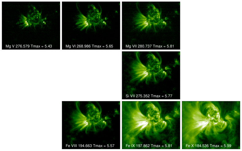
Figure 1.— Hinode EIS rasters of AR 10978 showing the similarity of Fe VIII and Si VII images. The Mg VI and Fe IX images look to be formed at lower and higher temperatures, respectively. For example, note the increasing vertical extent of the fan structures and cool features to east and west of the active region as you look at the images from top to bottom of the third column (Mg VI, Si VII, Fe IX). The images are scaled linearly.

A class of loops that have not yet been studied in sufficient detail with the latest instrumentation are the fan structures that appear as partially observed long loops at the edges of active regions. They are seen mostly in the 0.4–1.3MK temperature range (Schrijver et al., 1999; Del Zanna & Mason, 2003; Ugarte-Urra et al., 2009) and have densities greater than $\log\,(N_{e}/cm^{-3})$ = 9 (Del Zanna, 2003; Young et al., 2007b). They also appear to show red-shifted downflows (Winebarger et al., 2002; Marsch et al., 2004). We examine a sample of these structures in this paper.

For this and all the above observational studies, spectral emission from ions of Fe is of major importance. The high elemental abundance of Fe leads to many strong emission lines in spectrometer and imager pass-bands, yet interpretation of the observations is often difficult because of uncertainties in the atomic data used in prediction of emission (Lanzafame et al., 2002; Young et al., 2009). In principle, the emission from spectral lines of Fe can provide stringent constraints on temperatures and densities in the corona, however, it is of paramount importance that the diagnostic capabilities of Fe lines be assessed critically.

Initial results from EIS have indicated a number of problems in interpreting the Fe emission. Young et al. (2007b) noted that spectroheliograms of Fe VIII and Si VII look very similar in specific active region features such as the fan loops, despite the fact that the temperatures of the peak fractional abundance in ionization equilibrium are significantly different; $\log\,(T_{e}/K)$ = 5.6 and 5.8, respectively, according to Mazzotta et al. (1998). Since Fe is a considerably more complex atom than Si and is therefore likely to be less well understood, this observation has led to the suggestion that the ionization balance calculations for Fe VIII need to be revised upward to higher temperatures (Young et al., 2007b). Furthermore, this could have an impact on surrounding ions such as Fe VII and Fe IX. Recently, Young & Landi (2009) found evidence that this is indeed the case for Fe VII.

In addition to this temperature problem, a number of previous differential emission measure (DEM) studies have found difficulties reproducing the absolute intensities of Fe VIII and Si VII lines simultaneously. See, for example, the quiet Sun off-limb DEM analysis of Warren & Brooks (2009), the on disk quiet Sun study of Brooks et al. (2009), or the analysis of a cool active region feature by Landi & Young (2009).

Such issues are important to resolve as the Fe VIII 185.213 Å  and Si VII 275.368 Å  lines would provide the best EIS lower temperature constraints on the DEM if we had good confidence in the atomic data. Also, since they are strong, they are the best lines to use for velocity measurements in the transition region, and are present in the majority of EIS observations. As discussed, it is therefore of critical importance that we have confidence in the temperatures we assign to the measured velocities.

Changes to the formation temperatures or atomic data for these ions could also have an impact on interpreting the results from imagers. For example, changes to Fe VIII could affect the response functions for the 131 Å  channel of the Atmospheric Imaging Assembly (AIA) on the Solar Dynamics Observatory (SDO).

Motivated by our interest in studying the temperature and velocity structure of the fan loops, this situation has led us to take a closer look at the formation of the Fe VIII and Si VII spectral lines. Recently, there have been a number of revisions to the ionization balance calculations (Bryans et al., 2009; Dere et al., 2009) and we investigate whether they could help resolve these inconsistencies. We also examine the details of spectral line formation in this temperature range in the quiet Sun and in the fan loops. In particular, we examine whether convolving the contribution functions with the temperature distribution of the feature could explain the similarity of Fe VIII and Si VII images. It is known that the temperature of peak contribution to the line intensity can be shifted from the theoretical peak temperature of the emissivity if the shape of the DEM is taken into consideration (Brosius et al., 1996; Feldman et al., 1999; Del Zanna et al., 2003). In doing so, we finally show that the ionization equilibrium calculations for Fe may not be the source of this problem. By determining more realistic effective formation temperatures, we present a possible explanation for the observations. We also show that the most recent ionization balance calculations can resolve the discrepancies in the magnitudes of the intensities found in previous studies.

With confidence in the atomic data for these ions restored, we perform an emission measure (EM) analysis of a number of fan loops using EIS and AIA and compare the results from the two instruments.

2. Similarity of Fe VIII and Si VII images

Figure 1 shows example images of AR 10978 in (top left to bottom right) Mg V 276.579 Å, Mg VI 268.986 Å, Mg VII 280.737 Å, Si VII 275.368 Å, Fe VIII 194.663 Å, Fe IX 197.862 Å, and Fe X 184.536 Å. These images are formed at $\log\,(T_{e}/K)$ = 5.4, 5.6, 5.8, 5.8, 5.6, 5.8, and 6.0, respectively, according to Mazzotta et al. (1998). The data were obtained on 2007, December 10, at 00:19:27UT. The EIS instrument has 4 slit options (1^′′, 2^′′, 40^′′, and 266^′′). The 1^′′ slit was used for these observations and stepped over a FOV of 460^′′ by 384^′′. The exposure time was 40s at each position. The data were processed using standard EIS data reduction routines available in SolarSoft (eis_prep).

It is clear that the images do not follow the expected temperature trend. The Fe VIII and Si VII images look very similar, especially in the fan structures to solar east of the AR and the cool loops to solar west. This suggests a similar temperature of formation. In addition, the Mg VI and Fe IX images look to be formed at lower and higher temperatures, respectively. Note, for example, the third column of the figure. The vertical extent of the cool features to solar west and the fan structures to solar east appears to increase from top to bottom (Mg VI to Si VII to Fe IX) suggesting an increase in temperatures. The problem identified by Young et al. (2007b) is clearly seen in these examples.

3. Atomic Data

In this work we use several sources of atomic data as follows. All the contribution functions are calculated using the CHIANTI v6.0.1 database (Dere et al., 1997, 2009). The coronal abundances of Feldman et al. (1992) were used, together with the ionization fractions of Mazzotta et al. (1998) and Dere et al. (2009).

We use four specific lines to explore how their formation temperatures change in the quiet Sun: Mg VI 268.986 Å, Fe VIII 185.213 Å, Si VII 275.368 Å, and Fe IX 188.485 Å. For these lines we used the effective collision strengths and radiative data of Landi & Bhatia (2007), Griffin et al. (2000), Bhatia & Landi (2003), and Storey et al. (2002), respectively. A large number of additional spectral lines were used to compute DEMs and the data sources for these secondary data are too numerous to list here. We refer the interested reader to the CHIANTI database where the references are given in detail.

4. Spectral Line Formation Temperatures

The intensity of an optically thin emission line arising from an atomic transition from level $i$ to level $j$ can be expressed as

$$I_{ij}=\int_{T_{e}}G_{ij}(T_{e},N_{e})\phi(T_{e})dT_{e}$$ (1)

where the differential emission measure (DEM) is defined as,

$$\phi(T_{e})=N_{e}^{2}dz/dT_{e}$$ (2)

with $dz$ the differential distance along the line of sight and $N_{e}$ the electron density. The contribution function is defined as

$$G_{ij}(T_{e},N_{e})=A(Z)F(T_{e},N_{e})\epsilon_{ij}(T_{e},N_{e}){n_{H}\over(4\pi N_{e}^{2})}$$ (3)

with $A(Z)$ the elemental abundance, $n_{H}$ the hydrogen number density, $\epsilon_{ij}(T_{e},N_{e})$ the line emissivity normalized to the ground state population, and $F(T_{e},N_{e})$ the ionization fraction as a function of temperature and density. The accuracy of the computation of $F$ for Fe and Si is important for this paper. In Figure 2 we contrast the Mazzotta et al. (1998) ionization equilbrium calculations for Fe VIII and Si VII with the updated results of Dere et al. (2009). Note that the peak formation temperature does not change, so the temperature problem remains. The maximum fractional abundance, however, increases by 10% for Si VII and 55% for Fe VIII. These changes could be important when modeling the magnitudes of the absolute intensities. Note that the Bryans et al. (2009) calculations give the same formation temperatures for Si VII and Fe VIII as Dere et al. (2009). The maximum fractional abundances are also within 10%.

Figure 2.— Comparison of the Fe VIII and Si VII ionization equilibrium curves calculated by Mazzotta et al. (1998) with those of Dere et al. (2009).

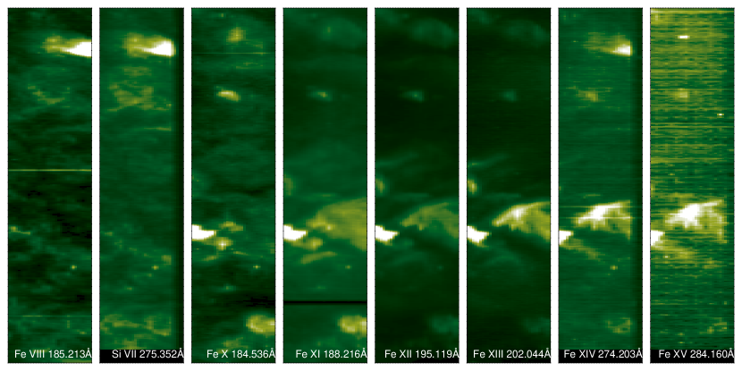
Figure 3.— Top row: Context observations of the quiet Sun region. From left to right, images in Fe VIII 185.213 Å, Si VII 275.368 Å, Fe X 184.536 Å, Fe XI 188.216 Å, Fe XII 195.119 Å, Fe XIII 202.044 Å, Fe XIV 274.203 Å, and Fe XV 284.160 Å. The images are scaled linearly between their minimum and maximum values, except for Fe XV which is scaled logarithmically because it is very weak. Images longward of 250 Å  have been shifted upward to account for the offsets between the EIS CCDs. The common area of the CCDs was averaged to compute the DEM. The Y-dimension has been rebinned for presentation. Lower row: Left panel, comparison between the quiet Sun DEM derived using the latest atomic data in this paper and that of Brooks et al. (2009). Right panel, normalized $g(T_{e},N_{e})$ function in the quiet Sun for Mg VI 268.986 Å, Fe VIII 185.213 Å, Si VII 275.368 Å, and Fe IX 188.485 Å. The lines are formed at $\log\,(T_{e}/K)$ = 5.68, 5.75, 5.85, and 6.05, respectively.

The function $G$ is strongly peaked at the characteristic temperature of the line, but the temperature of peak contribution to the total intensity can be shifted from the theoretical one if there is relatively more emitting material at higher or lower temperatures. Another key issue for this paper is that if the contribution function is broad, there may be significant contributions to the total intensity from multiple temperatures. In Figure 2, note that the Fe VIII curve is significantly broader than that of Si VII in the new Dere et al. (2009) calculation, and encompasses much of the temperature range of that ion. A further refinement to the analysis then, is to calculate the effective formation temperature (T_eff) of the line by convolving the contribution function with the DEM distribution for the target region or structure of interest, and then taking the temperature at which that function has its maximum value.

$$g(T_{eff},N_{e})=\max(g(T_{e},N_{e}))$$ (4)

where $g(T_{e},N_{e})$ is obtained by differentiating Equation 1, viz.

$$g(T_{e},N_{e})=G_{ij}(T_{e},N_{e})\phi(T_{e})$$ (5)

4.1. Formation Temperatures in the Quiet Sun

Before turning to the AR fan loops, we first investigate the formation temperatures of lines in the quiet Sun. Since we are also interested in how the more recent ionization balance calculations affect the derived DEM, and whether they could help in resolving known discrepancies, we derived a new QS DEM using the latest updated atomic data from v6.0.1 of the CHIANTI database and adopting the ionization fractions calculated by Dere et al. (2009). Throughout this paper we use the pre-launch laboratory photometric calibration of EIS (Lang et al., 2006).

Perhaps the best way to test the accuracy of the atomic data is to use off-limb QS observations where there is less contamination along the line of sight from multiple temperatures. Therefore, we selected lines for analysis that were identified as yielding consistent emission measure distributions above the quiet solar limb. Most of them are taken from Table 4 of Warren & Brooks (2009). The critical issue here, however, is the consistency of lines in the temperature range where Fe VIII, Fe IX, and Si VII are formed, and it would be best if we had independent constraints on the DEM that do not involve these lines. Therefore, we used deep exposure observations of an on-disk QS dataset. Deep exposure data are helpful for bringing out the weaker cool lines below $\log\,(T_{e}/K)$ = 5.8, that would be harder to detect off-limb, and therefore for constraining the DEM at the lower temperature end. This also allows us to directly compare the results to that of Brooks et al. (2009) where various inconsistencies in observed and predicted intensities were found in on-disk data using the older ionization balance calculations.

The data used were taken on 2009 June 14 starting at 09:59:42UT. Context images of the quiet region are shown in Figure 3 including both Si VII 275.368 Å  and Fe VIII 185.213 Å, which again look very similar. The EIS study used the 2^′′ slit with 4 min exposures and scanned a FOV of 60${}^{\prime\prime}\times$ 512^′′ in about 2hrs 10 mins. About 70% of the wavelength range of the CCDs were read-out and telemetered to the ground. Since this does not cover the full CCD, some of the lines used in Warren & Brooks (2009) were not available. In addition, we included several important lines of interest for this work, i.e., Mg VI 268.986 Å, Fe VIII 185.213 Å, and Si VII 275.368 Å, and, as discussed, additional cooler temperature lines to provide constraints on the DEM (O IV 279.631 Å, O IV 279.933 Å, O V 248.456 Å, Fe VIII 186.601 Å, Fe VIII 194.663 Å, Si VII 272.641 Å, Mg VII 278.402 Å, and Mg VII 280.737 Å). All the lines used are listed in Table 1 which also shows which lines were selected for the analysis of the fan loops in Sections 5 and 6.

The data were processed using standard procedures available in SolarSoft. In addition, however, the orbital variation of the line centroids and spectral line tilt were estimated by single Gaussian fits to the Fe XII 195.119 Å  line and removed from the data prior to further analysis. The offsets in X- and Y- between the short and long wavelength CCDs were corrected for so that the same area was averaged. These offsets were estimated using the software developed by Young et al. (2009). The data were then averaged over the common area of the two CCDs and fitted using single or multiple Gaussians as appropriate.

4.2. Differential Emission Measure

The method for determination of the DEM distribution is the same as described in Warren (2005), Brooks & Warren (2006), and Brooks et al. (2009). Briefly, we represent the DEM with a series of spline knots, the magnitudes of which are found by $\chi^{2}$ minimization of the differences between the observed and DEM predicted intensities. This minimization is performed by the SolarSoft routine MPFIT (Markwardt, 2009). The number and initial values of the spline knots can be pre-set and they can be interactively manipulated to control the smoothness of the emission measure. This technique has been found to be useful for representing rapid changes in the DEM.

We measured the electron density using the following three line ratios: Fe XIII 196.525 Å/202.044 Å, Fe XIII 202.044 Å/203.826 Å, and Fe XII 186.880 Å/195.119 Å. There are a number of issues with blending and the accuracy of the atomic data within certain ranges for these diagnostic ratios that are discussed in detail by Young et al. (2009). None of these issues are expected to affect our measurements significantly, however. The ratios give densities for the quiet Sun of $\log\,(N_{e}/cm^{-3})$ = 8.7–9.0, indicating a pressure of $\log\,(P_{e}/cm^{-3}K^{-1})$ = 14.9–15.2. The upper ends of these ranges are from Fe XII, which tends to give higher values (Young et al., 2009). Since we cannot rule out that the possibility that this is a real density change with temperature, we choose to assume that the electron pressure is constant. One of these assumptions is necessary to cast the intensity integral in the form of Equation 1 and calculate the contribution functions. We adopt a value of $\log\,(P_{e}/cm^{-3}K^{-1})$ = 15.0 in this work and compute the contribution functions for all the emission lines of Table 1 using CHIANTI.

The quiet Sun DEM of Brooks et al. (2009) was used to give a first guess for the temperature knots and spline fit to the QS data. The fit was then adjusted slightly to improve the agreement between observed and predicted intensities. The results are given in Table 1 and shown in comparison with our previous result in Figure 3. 80% of the lines are reproduced to within 30%. Fe XIV 270.519 Å  and Fe XV 284.160 Å  are significantly overestimated but these lines are very weak in the spectrum and the DEM is falling rapidly in this temperature range. Fe XIII 200.021 Å, Fe XIV 264.787 Å, and Fe XIII 197.434 Å  are underestimated by the DEM but these results are consistent with our previous work, and the latter is blended with Fe VIII 197.362 Å  (Brown et al., 2008). Mg VII 278.402 Å  is underestimated by about a factor of two, but this discrepancy can be resolved if the contribution from the Si VII 278.445 Å  blend is accounted for as described in Young et al. (2007b).

All of the Fe VIII, Fe IX, and Si VII lines are consistent with each other and the predicted intensities are within 30% of the observed ones. These results are interesting because the DEM curve derived using the updated atomic data and ionization fractions from CHIANTI v6.0.1 resolves the inconsistencies found using older versions in several previous studies of Fe VIII and Si VII lines in the quiet Sun off limb, on disk, and in cool active region features (Warren & Brooks, 2009; Brooks et al., 2009; Landi & Young, 2009).

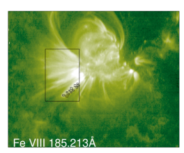
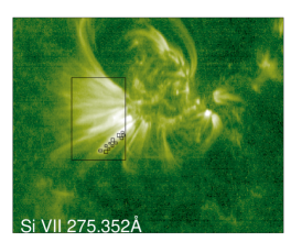
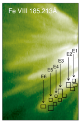
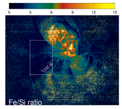
Figure 4.— Example showing the similarity of Fe VIII 185.213 Å  and Si VII 275.368 Å  images. A ratio map and histogram are shown indicating the low variation of the ratio across the fans. The histogram is made from the region indicated by the large box. An enlargment of the boxed region is also shown to highlight the locations used for the analysis along the fan loop (E1–E6). The adjacent boxes show the areas used for background subtraction.

Figure 5.— Emission measure results along the loop from the base (top left) to the top (bottom right) and the effect on the intensities of Fe VIII 185.213 Å  and Si VII 275.368 Å. Top two rows: temperature distribution with the peak temperature, emission measure, and Gaussian width indicated. Bottom two rows: Intensity of the two spectral lines as a function of temperature. The vertical dotted lines indicate the formation temperatures ($\log\,T_{max}$). The separation in formation temperatures is shown in the legend ($\Delta\log T$) and decreases towards the loop top.

4.3. Discussion

Using Equations 4 and 5 we determined T_eff in the quiet Sun for four key lines (Mg VI 268.986 Å, Fe VIII 185.213 Å, Si VII 275.368 Å, and Fe IX 188.485 Å). The gradient of the DEM slope in the quiet Sun increases in the temperature range of formation of these lines (Figure 3) so that there is relatively more material above the temperature of the maximum ion abundance for all of them. This results in all of these lines being formed at temperatures above their maximum ion abundance. As noted, however, the Fe VIII 185.213 Å  line is particulary sensitive to this because of the larger width of the $F(T_{e},N_{e})$ curve. It is therefore disproportionately affected, and is actually formed much closer in temperature to Si VII 275.368 Å  than the ionization balance would suggest. An illustrative example is shown in Figure 3. Note that the $g(T_{e},N_{e})$ curve for Fe VIII 185.213 Å  is considerably broader than for the other lines, suggesting that there will be contributions from multiple temperatures. Note also that because the contribution functions for individual lines differ within an ion they may also have different effective temperatures.

5. Formation Temperatures in Active Region Cool Fan Structures

In the previous section we discussed how the slope of the DEM could lead to the Fe VIII 185.213 Å  and Si VII 275.368 Å  lines being formed at similar temperatures in the quiet Sun. This DEM analysis was made, however, on averaged spectra over a relatively large area, and the differences may not be dramatic because the structure of the atmosphere does not change rapidly over the small temperature interval ($\log\,(T_{e}/K)$ = 5.75–5.85) where the lines are formed. It is clear, however, that specific features such as the cool fan loops look very similar in Si VII and Fe VIII images. It remains to be seen whether this explanation could hold for these specific features of interest.

To address this question we investigate the temperature distribution of the extended fan loops in AR 10978 (shown in Figure 1). This active region has previously been studied by several authors (Doschek et al., 2008; Brooks et al., 2008; Warren et al., 2008; Ugarte-Urra et al., 2009; Bryans et al., 2010; Brooks & Warren, 2011).

5.1. Context images and intensity ratio map

Context images of the region in both Fe VIII 185.213 Å, and Si VII 275.368 Å  are shown in Figure 4. As with the analysis of the QS, we corrected for the CCD offsets, orbital variation and spectral line tilt prior to further analysis. In this case we use the artificial neural network model of Kamio et al. (2010) to correct the orbital variation of the line centroids and grating tilt. The rest of the data processing was accomplished using standard procedures (eis_prep). The fan region is shown as a large box in Figure 4.

Also shown in Figure 4 is a map of the Fe VIII 185.213 Å/Si VII 275.368 Å  intensity ratio. This quantitatively describes the similarity of the two images. Note that the ratio appears to vary in the active region core. Fe VIII 185.213 Å  is blended with Ni XVI 185.251 Å  (Young et al., 2007a; Brown et al., 2008), which is formed at 2.8MK, and it likely contributes to this emission and influences the ratio. In contrast, one can see that the fan region is almost uniformly dark, indicating little variation in the ratio across this area. A histogram of the ratio values for the pixels within the boxed region is also shown in the Figure. A Gaussian fit to this distribution indicates that the mean value is 2.3 and the standard deviation is 0.34, i.e., the variation in the ratio across the fans is less than 15%.

5.2. EM analysis

We computed the emission measure in several small boxes extending along one of the fan loops (shown as regions E1–E6 in Figure 4). The intensities were averaged in these areas. The background emission was estimated for each box by averaging the intensities in the adjacent boxes also shown in the Figure. Single and multiple Gaussian fits were made as appropriate.

For this analysis we used most of the same lines as we used for the QS. These are indicated in Table 1. A few lines were not available in the current dataset and could not be included. These lines can also be identified from the Table. Furthermore, we included O VI 183.937 Å, O VI 184.117 Å, Fe XVI 262.984 Å, and Fe XVI 265.003 Å  to provide additional low and high temperature constraints.

Warren et al. (2008) analyzed a sample of ‘warm’ EUV loops in this region by fitting a Gaussian distribution in temperature for the model emission measure of the form,

$$\xi(T_{e})=\frac{EM_{0}}{\sigma_{T_{e}}\sqrt{2\pi}}\exp\left[-\frac{(T_{e}-T_{0})^{2}}{2\sigma_{T_{e}}^{2}}\right]$$ (6)

For comparison with this work we use the same fitting technique here. The fit is made by $\chi^{2}$ minimization of the differences between the measured and computed intensities. The density is allowed to be a free parameter in the fitting and we obtain values of $\log\,(N_{e}/cm^{-3})$ = 9.2–9.7, decreasing from base to apex. These results are comparable to the decrease along another example reported by Young et al. (2007b).

The computed temperature distributions for positions E1–E6 along the loop together with their peak temperatures, emission measure, and Gaussian width are shown in the top two rows of Figure 5. There are a few problematic lines that are not well reproduced by the model. They vary by position, but generally include O IV 279.933 Å, O V 248.456 Å, and O VI 183.937 Å, all of which are underestimated to varying degrees. Furthermore, the background subtracted high temperature lines of Fe XIV and Fe XVI are often underestimated, including the normally robust Fe XIII 202.044 Å  line. O V 248.456 Å  is blended with an Al VIII line that is a weak contributor in most conditions, hence the agreement found for O V in the QS. The blend, however, could contribute more when the emisison measure is peaked mostly at coronal temperatures. The Mg VII 278.402 Å  and 280.737 Å  lines also sometimes show unusual behavior. In most cases they are reproduced well, but mismatches of 50–80% are sometimes seen. In these cases, the discrepancies for Mg VII 278.402 Å  cannot be resolved by accounting for the blend with Si VII 278.445 Å. Since it is mostly the low and high temperature lines that show discrepancies it could be that the temperature distribution deviates from a Gaussian shape in the wings. In general most of the lines are reproduced well, however. In total, about 80% of the lines are reproduced to within 40% with most better than 30%.

5.3. Discussion

Compared to the quiet Sun, the fans show a significant enhancement of emission measure (factor of 3–7). The distribution peaks at $\log\,(T_{e}/K)$ = 6.0 near the base (E1) and increases along the loop to a maximum of $\log\,(T_{e}/K)$ = 6.1 (E3 and E4) before decreasing again. The dispersion in the Gaussian distribution appears to decrease along the loop length. Previous studies of cool loops in active regions have suggested that they are isothermal (Del Zanna & Mason, 2003). Our results indicate that at its narrowest, the width of the emission measure distribution is still $\log\,(\sigma_{T_{e}}/K)\approx$ 5.4. In comparison with the ‘warm’ loops in this region studied by Warren et al. (2008), this fan loop has a broader temperature distribution along most of its length. Only towards the tip (E6) does it approach the values for the ‘warm’ loops. Note that the gradient of the slope of the emission measure distribution in the temperature range $\log\,(T_{e}/K)$ = 5.6–5.8 is greater than in the quiet Sun, even at the base of the fan (E1).

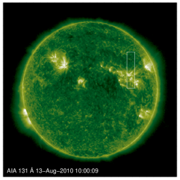
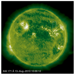
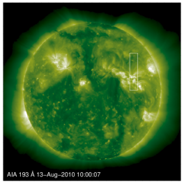
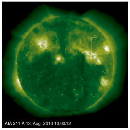
Figure 6.— Full Sun images from SDO in the AIA 133 Å, 171 Å, 193 Å, and 211 Å  filters. The overlaid box shows the FOV used in Figure 7.

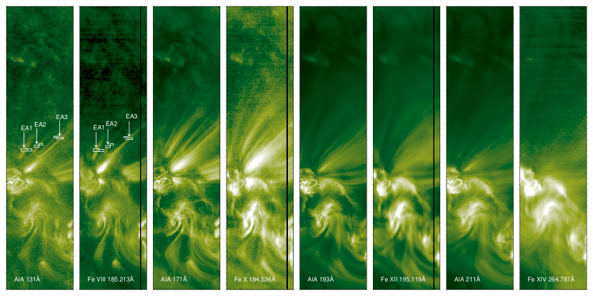
Figure 7.— AIA and EIS images of fan loops. From the left: AIA 133 Å, EIS Fe VIII 185.213 Å, AIA 171 Å, EIS Fe X 184.536 Å, AIA 193 Å, EIS Fe XII 195.119 Å, AIA 211 Å  filters, and EIS Fe XIV 264.787 Å. The images are scaled logarithmically.

Figure 5 also shows the normalized $g(T_{e},N_{e})$ function for the Fe VIII 185.213 Å, and Si VII 275.368 Å  lines that results from convolving their contribution functions with the fan emission measure at each position. We see that even when the temperature distribution is relatively broad (E1), the effective formation temperatures of the lines are separated by only 0.1 in the $\log$. It also indicates that the separation in temperatures reduces as we go along the fan loop until they are both formed at the same temperature of $\log\,(T_{eff}/K)$ = 5.85. Clearly when the EM distribution is narrow in this temperature range the two lines will be formed close together in temperature. This analysis also shows that this is true even if the EM distribution is relatively broad, provided it has a positive gradient. The Fe VIII 185.213 Å  line seems to be very sensitive to the slope of the EM distribution in general.

Figure 8.— Emission measure results for the three loops EA1, EA2, and EA3 from EIS and AIA and the effect on the intensities of Fe VIII 185.213 Å, Si VII 275.368 Å, and the AIA 131 Å  response function. Top row: EIS EM distributions. Second row: AIA EM distributions. EM loci curves are overlaid in color. Third row: Intensity of the two EIS spectral lines as a function of temperature. The vertical dotted lines indicate the formation temperatures. The separation in formation temperatures is shown in the legend. Bottom row: The AIA 131 Å  effective response as a function of temperature. The original response is shown by the dashed line.

6. Emission measure analysis with EIS and AIA

To examine whether our explanation could hold in general for all fan loops we investigated a number of other cases. The loops we selected were observed in active region 11093 on 2010, August 13. In this analysis, we also include data obtained by SDO/AIA (Golub, 2006). As mentioned in the introduction, it is also important to understand the formation of spectral lines in detail if we are to correctly interpret observations by EUV imagers. The broad wavelength pass-bands of such instruments include multiple lines and their contributions may change in quiet and active conditions. We illustrate this here by examining the temperature response of the AIA 131 Å  filter. The pass-band of this filter is expected to contain contributions from Fe VIII 130.941 Å  and 131.240 Å, Fe XX 132.850 Å, Fe XXI 128.755 Å, and Fe XXIII 132.906 Å  with the Fe VIII lines the dominant contributor outside of flares. As we have seen, the formation of Fe VIII lines is non-trivial.

Figure 6 shows full Sun images from AIA taken at 10UT. AR 11093 was the target for Hinode and the EIS FOV is overlaid as a box (120^′′ by 512^′′). The EIS observation started at 09:26:40 and lasted about 1 hour. During this time the 1^′′ slit was moved in steps of 2^′′ across the region with 60s exposures at each position. The EIS data were reduced and processed in the same way as discussed previously.

The AIA data were obtained pre-processed from the level 1.5 cutout service. These data have had flat-fielding and dark current corrections applied. Bad pixels and cosmic ray hits have also been repaired by an iterative method. We converted the data to DN/pixel/s. The images have also been rotated to solar North and shifted to match the SDO/HMI (Helioseismic and Magnetic Imager) FOV center so that they are all coaligned. Nevertheless, we detected some small offsets between different filters and corrected this misalignment by cross-correlating the full disk images.

Coalignment of the EIS and AIA data was achieved by extracting the EIS FOV from the AIA 131 Å  full Sun image and cross-correlating it with the Fe VIII 185.213 Å  EIS raster. Due to the orbital variation of the position of the EIS slit, the spatial sampling is not uniform across the raster. In contrast, the AIA image is taken nearly instantaneously (2.9s exposure) so there is negligible movement. Therefore, the effective plate-scale magnification between the images is not uniform in the solar X-direction. For these observations this discrepancy amounted to 1^′′ across half the raster and was corrected manually.

Figure 7 shows images from EIS and AIA of the EIS FOV. For this analysis we selected small boxes on each of 3 loops and averaged the intensities in these areas. The selected positions are shown in the figure as EA1, EA2, and EA3. The background emission was estimated for each box by averaging the emission in the adjacent boxes (also shown in the figure). Single and multiple Gaussian fits to the EIS data were made as appropriate. The spectral line-list for these observations was smaller than that of the December 2007 region, but it still covered a sufficiently broad temperature range from $\log(T_{e}/K)$ = 5.5 to 6.4. The selected lines are indicated in Table 1. In addition, we included O VI 184.117 Å, Mg V 276.579 Å, and Mg VI 270.394 Å  to provide further lower temperature constraints.

The emission measure analysis is the same as that used in the previous section for consistency. Since the background subtraction sometimes reduces the intensities of the density diagnostic lines to zero, we have assumed a density of $\log(N_{e}/cm^{-3})$ = 9.5 in computing the emission measure for both EIS and AIA. This value is the average of that obtained along the loop analyzed in §5.2.

We extracted intensities from the coaligned 131 Å, 171 Å, 193 Å, 211 Å, 335 Å, and 94 Å  filters. These filters are expected to be dominated by lines of Fe VIII, Fe IX, Fe XII, Fe XIV, Fe XVI, and Fe XVIII. The 94 Å  filter also contains contributions from Fe VIII and Fe X which can dominate under certain conditions (O’Dwyer et al., 2010). We use only the intensities that correlate well with the 131 Å  intensity for generating the emission measure distribution. In practise, this generally excludes the 335 Å  and 94 Å  bands where there is little emission for the fan loops we study. A photometric calibration uncertainty of 25% is used as the intensity error (Boerner et al., in preparation). The response functions were calculated for a grid of electron densities and temperatures spanning $\log\,(N_{e}/cm^{-3})$ = 6–12 and $\log\,(T_{e}/K)$ = 4–8. This was done by calculating isothermal spectra as a function of wavelength at each temperature and density, $S(\lambda,T_{e},N_{e})$, using CHIANTI v6.0.1 and the coronal abundances of Feldman et al. (1992). The spectra were then convolved with the effective areas for each filter, $E_{i}(\lambda)$, and integrated in wavelength, $\int E_{i}(\lambda)S(\lambda,T_{e},N_{e})d\lambda$, to obtain the response functions, $R_{i}(T_{e},N_{e})$. The effective areas were obtained from SolarSoft.

The EM distributions computed from the EIS data for EA1, EA2, and EA3 are shown in the top row of Figure 8. The results computed from the AIA data are shown in the second row. EM loci curves are also shown to indicate the sensitivity of the EIS lines and AIA filters. Table 2 shows the peak temperature ($\log T_{0}$), emission measure ($\log EM_{0}$), and Gaussian width ($\log\sigma_{0}$) derived from EIS and AIA for each loop. The uncertainties in these parameters are also given.

The two instruments agree that the peak temperatures of the loops are $\log\,(T_{e}/K)$ = 5.9–6.0. The emission measure magnitudes are $\log\,(EM/cm^{-5})$ = 26–27 and the EIS and AIA results are consistent to 25–55%. The EIS data indicate that one of the loops (EA1) is isothermal and that the other two have a finite (but narrow) width, consistent with the findings for the loop in §5.2. The AIA data yield similar results. For the two loops that are not isothermal, AIA finds a slightly larger thermal width (0.14 in $\log$). This may be due to the coarser temperature resolution compared to EIS. The uncertainties in all parameters from AIA are also larger. Note that an error of zero is returned in the isothermal case because the temperature becomes fixed.

Again in Figure 8 we show the intensities of Fe VIII 185.213 Å  and Si VII 275.368 Å  as a function of temperature after convolution with the EM distribution of each loop. In all three cases the two lines are effectively formed at the same temperature.

We also investigated the effective response of the AIA 131 Å  filter after convolution with the EIS emission measure distribution. The main contributing lines in this pass band at $\log\,(T_{e}/K)<$ 6.4 are Fe VIII 130.941 Å, and Fe VIII 131.240 Å. These produce the peak around $\log\,(T_{e}/K)$ = 5.7 in the usual response, $R_{131}(T_{e})$ (dashed line in Figure 8). The convolved function $R_{131}(T_{e})\xi(T_{e})T_{e}$ is plotted in Figure 8 as the solid line. Note that the peak of the response shifts to higher temperatures after being convolved with the EM distribution; $\log\,(T_{e}/K)$ = 5.85–5.95. This is consistent with the analysis in the previous sections and demonstrates that these effects can also be important for imager observations.

7. Summary

Motivated by the desire to study the temperature structure of active region fan loops we have attempted to resolve inconsistencies found in previous work using EIS data. In particular, we have shown that the similarity in EIS Fe VIII 185.213 Å  and Si VII 275.368 Å  images, that is not expected from the respective temperatures of peak abundance in ionization equilibrium, can be understood when a more accurate calculation of the effective formation temperature in the solar corona is performed. This is done by convolving the contribution functions with the DEM of the target of interest. If the DEM has a steep gradient in the $\log\,(T_{e}/K)$ = 5.6–5.8 range, or is sharply peaked, the two lines will be formed close in temperature. In this work, we compared the effect of this technique on the formation temperatures of these lines in the quiet Sun. The initial separation of $\log\,(T_{e}/K)$ = 5.6–5.8 is reduced to 5.75–5.85, and it is clear that Fe VIII 185.213 Å  has a substantial contribution from emitting material at $\log\,(T_{e}/K)$ = 5.8.

To examine whether this explanation could work for the fan loops, we derived the EM distribution along one example in AR 10978. The temperature distribution peaks near 1–1.2MK and narrows along the loop. The peak contribution to the line intensity is $\log\,(T_{e}/K)$ = 5.9 for both the Fe VIII 185.213 Å  and Si VII 275.368 Å  lines. To investigate whether this effect is generally applicable to other AR fans, we examined a number of other loops. We found that in all cases the two lines are formed at the same temperature ($\log\,T_{e}/K\sim$ 5.9). This suggests therefore, that the expected difference in images of the fans formed from these lines is a result of an overestimation of the separation in formation temperatures by the approximate method of assuming the lines are formed at the temperature of the peak fractional abundance in ionization equilibrium.

Note that other lines may be affected in similar ways. For example, in Figure 1 the Mg VII and Fe IX images look different despite the fact that they have similar ionization equilibrium temperatures. We have verified that they are in fact formed at different temperatures in the fan loop of Section 5.

To demonstrate the importance of understanding the formation of the EUV spectrum for broad pass-band imagers we studied the effect of convolving the AIA 131 Å  response function with our EIS fan loop EM distributions. We showed that, as a result, the peak of the dominant lower temperature part of the effective response function shifts up to $\log\,(T_{e}/K)\sim$ 5.9.

It is important to emphasize that we have not shown that this explanation holds in general for all active areas or structures on the Sun. If the DEM slope is shallower (or flat) in the $\log\,(T_{e}/K)$ = 5.6–5.8 range then the Fe VIII 185.213 Å  and Si VII 275.368 Å  lines should still be formed at a wider separation in temperatures and examples of significantly different images should be found. The apparent lack of such observations for any solar feature, however, provides a stringent constraint on the gradient of the DEM slope in this temperature range all over the Sun. This is consistent with other independent studies that show strong similarities in the shape of the DEM distribution in different areas of the quiet Sun (Lanzafame et al., 2005; Brooks et al., 2009; Feldman et al., 2009).

The DEM-gradient resolves the inconsistencies in formation temperatures between the Fe VIII and Si VII lines, but a related issue is that discrepancies have also been found in the magnitude of the intensities of these lines in previous DEM studies using EIS data. We showed here that these additional issues are resolved when the most recent ionization balance compilation data of Dere et al. (2009) are used for the atomic calculations. From this analysis, therefore, no substantive relative error in the Fe ionization balance is indicated for the specific ions of Fe VIII and Fe IX.

This work has demonstrated that the strong Fe VIII 185.213 Å  and Si VII 275.368 Å  lines can be used with confidence for DEM studies and velocity work in the transition region. Therefore, we examined the temperature structure of a small sample of fan loops. We found that they have peak temperatures in the range 0.8–1.2MK. One loop was found to be isothermal, but more often the temperature distribution has a narrow width. This result is similar to that found by Warren et al. (2008) for ‘warm’ active region loops. In one detailed case, the EM distribution is found to broaden considerably towards the base. This could have implications for the location of the heating.

We also found that the peak temperatures and emission measures derived from AIA data are in agreement with those derived from EIS. There is also agreement on whether the loops are isothermal or not. The AIA analysis indicates a slightly larger thermal width than EIS when the loops are not isothermal. This is possibly because the EIS data contain observations from consecutive ionization stages of Fe  whereas the AIA data only sample every second ionization stage.

Table 1Quiet Sun intensities and line selection.

Ion	$\lambda_{obs}$ (Å)	I${}_{obs}^{a}$		I${}_{dem}^{a}$	Ratio	EQS	Efan	EAfan
O IV	279.631	1.82$\pm$	0.40	2.03	1.12	$\surd$
O IV	279.933	3.90$\pm$	0.86	4.06	1.04	$\surd$	$\surd$
O V	248.456	4.55$\pm$	1.00	4.23	0.93	$\surd$	$\surd$
FE VIII	185.213	28.55$\pm$	6.28	35.70	1.25	$\surd$	$\surd$	$\surd$
FE VIII	186.601	21.50$\pm$	4.73	24.37	1.13	$\surd$	$\surd$	$\surd$
FE VIII	194.663	7.79$\pm$	1.71	6.23	0.80	$\surd$	$\surd$
Mg VI	268.986	1.21$\pm$	0.27	1.48	1.22	$\surd$	$\surd$
Si VII	272.641	4.28$\pm$	0.94	4.48	1.05	$\surd$
Si VII	275.352	14.14$\pm$	3.11	14.58	1.03	$\surd$	$\surd$	$\surd$
Mg VII	278.402	15.81$\pm$	3.48	9.01	0.57	$\surd$	$\surd$	$\surd$
Mg VII	280.737	2.22$\pm$	0.49	2.83	1.27	$\surd$	$\surd$
FE IX	188.485	21.87$\pm$	4.81	23.66	1.08	$\surd$	$\surd$	$\surd$
Fe IX	189.941	11.38$\pm$	2.50	14.13	1.24	$\surd$
FE IX	197.858	15.15$\pm$	3.33	15.91	1.05	$\surd$	$\surd$	$\surd$
FE X	184.536	74.42$\pm$	16.37	63.20	0.85	$\surd$	$\surd$	$\surd$
Fe XI	180.401	139.19$\pm$	30.62	169.40	1.22	$\surd$
FE XI	182.167	23.31$\pm$	5.13	29.01	1.24	$\surd$	$\surd$
FE XI	188.216	75.23$\pm$	16.55	81.34	1.08	$\surd$	$\surd$	$\surd$
Fe XI	192.813	21.37$\pm$	4.70	16.99	0.80	$\surd$	$\surd$	$\surd$
FE XII	186.880	14.63$\pm$	3.22	15.11	1.03	$\surd$	$\surd$	$\surd$
Fe XII	192.394	20.17$\pm$	4.44	26.27	1.30	$\surd$	$\surd$	$\surd$
Fe XII	193.509	41.03$\pm$	9.03	55.33	1.35	$\surd$	$\surd$
FE XII	195.119	63.04$\pm$	13.87	82.05	1.30	$\surd$	$\surd$	$\surd$
FE XII	196.640	5.62$\pm$	1.24	4.82	0.86	$\surd$	$\surd$
FE XIII	196.525	0.76$\pm$	0.17	0.90	1.18	$\surd$	$\surd$
Fe XIII	197.434	4.10$\pm$	0.90	1.07	0.26	$\surd$
Fe XIII	200.021	4.15$\pm$	0.91	3.18	0.77	$\surd$
FE XIII	202.044	26.08$\pm$	5.74	21.47	0.82	$\surd$	$\surd$	$\surd$
FE XIII	203.826	10.98$\pm$	2.42	10.15	0.92	$\surd$	$\surd$	$\surd$
FE XIV	264.787	4.76$\pm$	1.05	3.39	0.71	$\surd$	$\surd$	$\surd$
Fe XIV	270.519	0.82$\pm$	0.18	2.14	2.61	$\surd$		$\surd$
FE XIV	274.203	4.78$\pm$	1.05	4.37	0.91	$\surd$	$\surd$
FE XV	284.160	1.97$\pm$	0.43	5.95	3.02	$\surd$	$\surd$	$\surd$
Mg V	276.579							$\surd$
Mg VI	270.394							$\surd$
O VI	183.977						$\surd$
O VI	184.117						$\surd$	$\surd$
Fe XVI	262.984						$\surd$
Fe XVI	265.003						$\surd$

Table 2Comparison of DEM results from EIS and AIA.

	EIS						AIA
Loop	$\log T_{0}$		$\log EM_{0}$		$\log\sigma_{0}$		$\log T_{0}$		$\log EM_{0}$		$\log\sigma_{0}$
EA 1	5.93$\pm$	0.01	27.10$\pm$	0.02	4.50$\pm$	0.00	5.88$\pm$	0.05	27.18$\pm$	0.07	4.50$\pm$	0.00
EA 2	5.90$\pm$	0.04	25.88$\pm$	0.09	5.41$\pm$	0.18	5.97$\pm$	0.13	26.10$\pm$	0.10	5.55$\pm$	0.20
EA 3	6.05$\pm$	0.01	26.44$\pm$	0.02	5.46$\pm$	0.04	6.03$\pm$	0.08	26.33$\pm$	0.10	5.60$\pm$	0.27

References

- Aschwanden (2002) Aschwanden, M. J. 2002, ApJ, 580, L79
- Aschwanden et al. (1999) Aschwanden, M. J., Newmark, J. S., Delaboudinière, J.-P., Neupert, W. M., Klimchuk, J. A., Gary, G. A., Portier-Fozzani, F., & Zucker, A. 1999, ApJ, 515, 842
- Aschwanden et al. (2008) Aschwanden, M. J., Nitta, N. V., Wuelser, J., & Lemen, J. R. 2008, ApJ, 680, 1477
- Bhatia & Landi (2003) Bhatia, A. K., & Landi, E. 2003, ApJ, 585, 587
- Brooks et al. (2008) Brooks, D. H., Ugarte-Urra, I., & Warren, H. P. 2008, ApJ, 689, L77
- Brooks & Warren (2006) Brooks, D. H., & Warren, H. P. 2006, ApJS, 164, 202
- Brooks & Warren (2009) Brooks, D. H., & Warren, H. P. 2009, ApJ, 703, L10
- Brooks & Warren (2011) Brooks, D. H., & Warren, H. P. 2011, ApJ, 727, L13
- Brooks et al. (2009) Brooks, D. H., Warren, H. P., Williams, D. R., & Watanabe, T. 2009, ApJ, 705, 1522
- Brosius et al. (1996) Brosius, J. W., Davila, J. M., Thomas, R. J., & Monsignori-Fossi, B. C. 1996, ApJS, 106, 143
- Brown et al. (2008) Brown, C. M., Feldman, U., Seely, J. F., Korendyke, C. M., & Hara, H. 2008, ApJS, 176, 511
- Bryans et al. (2009) Bryans, P., Landi, E., & Savin, D. W. 2009, ApJ, 691, 1540
- Bryans et al. (2010) Bryans, P., Young, P. R., & Doschek, G. A. 2010, ApJ, 715, 1012
- Cargill (1995) Cargill, P. J. 1995, in Infrared tools for solar astrophysics: What’s next?, ed. J. R. Kuhn & M. J. Penn, 17
- Culhane et al. (2007) Culhane, L., et al. 2007, PASJ, 59, 751
- Del Zanna (2003) Del Zanna, G. 2003, A&A, 406, L5
- Del Zanna (2008) Del Zanna, G. 2008, A&A, 481, L49
- Del Zanna et al. (2003) Del Zanna, G., Bromage, B. J. I., & Mason, H. E. 2003, A&A, 398, 743
- Del Zanna & Mason (2003) Del Zanna, G., & Mason, H. E. 2003, A&A, 406, 1089
- Dere et al. (1997) Dere, K. P., Landi, E., Mason, H. E., Monsignori Fossi, B. C., & Young, P. R. 1997, A&AS, 125, 149
- Dere et al. (2009) Dere, K. P., Landi, E., Young, P. R., Del Zanna, G., Landini, M., & Mason, H. E. 2009, A&A, 498, 915
- Doschek et al. (2007) Doschek, G. A., et al. 2007, ApJ, 667, L109
- Doschek et al. (2008) Doschek, G. A., Warren, H. P., Mariska, J. T., Muglach, K., Culhane, J. L., Hara, H., & Watanabe, T. 2008, ApJ, 686, 1362
- Feldman et al. (2009) Feldman, U., Dammasch, I. E., & Landi, E. 2009, ApJ, 693, 1474
- Feldman et al. (1999) Feldman, U., Doschek, G. A., Schühle, U., & Wilhelm, K. 1999, ApJ, 518, 500
- Feldman et al. (1992) Feldman, U., Mandelbaum, P., Seely, J. F., Doschek, G. A., & Gursky, H. 1992, ApJS, 81, 387
- Golub (2006) Golub, L. 2006, Space Sci. Rev., 124, 23
- Griffin et al. (2000) Griffin, D. C., Pindzola, M. S., & Badnell, N. R. 2000, A&AS, 142, 317
- Hara et al. (2008) Hara, H., Watanabe, T., Harra, L. K., Culhane, J. L., Young, P. R., Mariska, J. T., & Doschek, G. A. 2008, ApJ, 678, L67
- Kamio et al. (2010) Kamio, S., Hara, H., Watanabe, T., Fredvik, T., & Hansteen, V. H. 2010, Sol. Phys., 266, 209
- Klimchuk (2006) Klimchuk, J. A. 2006, Sol. Phys., 234, 41
- Kosugi et al. (2007) Kosugi, T., et al. 2007, Sol. Phys., 243, 3
- Landi & Bhatia (2007) Landi, E., & Bhatia, A. K. 2007, Atomic Data and Nuclear Data Tables, 93, 1
- Landi & Young (2009) Landi, E., & Young, P. R. 2009, ApJ, 706, 1
- Lang et al. (2006) Lang, J., et al. 2006, Appl. Opt., 45, 8689
- Lanzafame et al. (2005) Lanzafame, A. C., Brooks, D. H., & Lang, J. 2005, A&A, 432, 1063
- Lanzafame et al. (2002) Lanzafame, A. C., Brooks, D. H., Lang, J., Summers, H. P., Thomas, R. J., & Thompson, A. M. 2002, A&A, 384, 242
- Lenz et al. (1999) Lenz, D. D., Deluca, E. E., Golub, L., Rosner, R., & Bookbinder, J. A. 1999, ApJ, 517, L155
- Markwardt (2009) Markwardt, C. B. 2009, in ASP Conf. Series, ed. D. A. Bohlender, D. Durand, & P. Dowler, Vol. 411, 251
- Marsch et al. (2004) Marsch, E., Wiegelmann, T., & Xia, L. D. 2004, A&A, 428, 629
- Martens et al. (2002) Martens, P. C. H., Cirtain, J. W., & Schmelz, J. T. 2002, ApJ, 577, L115
- Mazzotta et al. (1998) Mazzotta, P., Mazzitelli, G., Colafrancesco, S., & Vittorio, N. 1998, A&AS, 133, 403
- O’Dwyer et al. (2010) O’Dwyer, B., Del Zanna, G., Mason, H. E., Weber, M. A., & Tripathi, D. 2010, A&A, 521, A21
- Parker (1983) Parker, E. N. 1983, ApJ, 264, 642
- Parker (1988) Parker, E. N. 1988, ApJ, 330, 474
- Patsourakos & Klimchuk (2006) Patsourakos, S., & Klimchuk, J. A. 2006, ApJ, 647, 1452
- Patsourakos & Klimchuk (2009) Patsourakos, S., & Klimchuk, J. A. 2009, ApJ, 696, 760
- Reale (2010) Reale, F. 2010, Living Reviews in Solar Physics, 7, 5
- Reale et al. (2009) Reale, F., Testa, P., Klimchuk, J. A., & Parenti, S. 2009, ApJ, 698, 756
- Schmelz et al. (2009) Schmelz, J. T., Saar, S. H., DeLuca, E. E., Golub, L., Kashyap, V. L., Weber, M. A., & Klimchuk, J. A. 2009, ApJ, 693, L131
- Schmelz et al. (2001) Schmelz, J. T., Scopes, R. T., Cirtain, J. W., Winter, H. D., & Allen, J. D. 2001, ApJ, 556, 896
- Schrijver et al. (1999) Schrijver, C. J., et al. 1999, Sol. Phys., 187, 261
- Storey et al. (2002) Storey, P. J., Zeippen, C. J., & Le Dourneuf, M. 2002, A&A, 394, 753
- Testa et al. (2010) Testa, P., Reale, F., Landi, E., DeLuca, E., & Kashyap, V. 2010, ArXiv e-prints
- Tripathi et al. (2010) Tripathi, D., Mason, H. E., & Klimchuk, J. A. 2010, ApJ, 723, 713
- Ugarte-Urra et al. (2009) Ugarte-Urra, I., Warren, H. P., & Brooks, D. H. 2009, ApJ, 695, 642
- Warren (2005) Warren, H. P. 2005, ApJS, 157, 147
- Warren & Brooks (2009) Warren, H. P., & Brooks, D. H. 2009, ApJ, 700, 762
- Warren et al. (2010) Warren, H. P., Brooks, D. H., & Winebarger, A. R. 2010, ArXiv e-prints
- Warren et al. (2008) Warren, H. P., Ugarte-Urra, I., Doschek, G. A., Brooks, D. H., & Williams, D. R. 2008, ApJ, 686, L131
- Winebarger et al. (2002) Winebarger, A. R., Warren, H., van Ballegooijen, A., DeLuca, E. E., & Golub, L. 2002, ApJ, 567, L89
- Young et al. (2007a) Young, P. R., et al. 2007a, PASJ, 59, 857
- Young et al. (2007b) Young, P. R., Del Zanna, G., Mason, H. E., Doschek, G. A., Culhane, L., & Hara, H. 2007b, PASJ, 59, 727
- Young & Landi (2009) Young, P. R., & Landi, E. 2009, ApJ, 707, 173
- Young et al. (2009) Young, P. R., Watanabe, T., Hara, H., & Mariska, J. T. 2009, A&A, 495, 587