Stability of the Parisi Solution for the Sherrington-Kirkpatrick model near $T=0$

Abstract

To test the stability of the Parisi solution near $T=0$, we study the spectrum of the Hessian of the Sherrington-Kirkpatrick model near $T=0$, whose eigenvalues are the masses of the bare propagators in the expansion around the mean-field solution. In the limit $T\ll 1$ two regions can be identified. In the first region, for $x$ close to $0$, where $x$ is the Parisi replica symmetry breaking scheme parameter, the spectrum of the Hessian is not trivial and maintains the structure of the full replica symmetry breaking state found at higher temperatures. In the second region $T\ll x\leq 1$ as $T\to 0$, the components of the Hessian become insensitive to changes of the overlaps and the bands typical of the full replica symmetry breaking state collapse. In this region only two eigenvalues are found: a null one and a positive one, ensuring stability for $T\ll 1$. In the limit $T\to 0$ the width of the first region shrinks to zero and only the positive and null eigenvalues survive. As byproduct we enlighten the close analogy between the static Parisi replica symmetry breaking scheme and the multiple time-scales approach of dynamics, and compute the static susceptibility showing that it equals the static limit of the dynamic susceptibility computed via the modified fluctuation dissipation theorem.

1 Introduction:

The physics of spin glasses is still an active field of research because the methods and techniques developed to analyze the static and dynamic properties have found application in a variety of others fields of the complex system world, such as neural networks or combinatorial optimization or glass physics. In the study of spin glasses a central role is played by the Sherrington-Kirkpatrick (SK) model [1], introduced in the middle of 70’s, as a mean-field model for spin glasses. Despite its solution, known as the “Parisi solution” [2, 3, 4], was found $30$ years ago, some aspect are still far from being completely understood. In this work we discuss the spectrum of the Hessian of the fluctuations for the Parisi solution in the limit of vanishing temperature, a still not fully explored problem.

The Hessian spectrum plays a central role non only for the stability of the Parisi solution of the mean-field SK model, but also for the study of finite dimensional systems. Its eigenvalues are indeed the masses of the “bare” propagators in the loop expansion about the mean-field limit. Thus the knowledge of the Hessian spectrum of the SK model is a prerequisite for any theory obtained from a development about the mean-field limit.

The stability of Parisi solution for the SK model near its critical temperature $T_{c}$, has been established long ago [5, 6] by exhibiting the eigenvalues of the Hessian matrix. In few words, one has a Replicon band whose lowest eigenvalues are zero modes, and a Longitudinal-Anomalous (LA) band, sitting at $(T_{c}-T)$, of positive eigenvalues (both with) a band width of order $(T_{c}-T)^{2}$. The analysis was partially extended later [7] via the derivation of Ward-Takahashi identities, showing that the zero Replicon modes would remain null in the whole low temperature phase, and hence would not ruin the stability under loop corrections to the mean-field solution.

Despite these efforts a complete analysis of the stability in the zero temperature limit is still missing. Near $T_{c}$ one can take advantage of the vanishing of the order parameter for $T=T_{c}$ and expand the free energy, a simplification clearly missing close to zero temperature, where the order parameter stays finite. Moreover the $T=0$ limit is highly non-trivial. All these make the derivation of “effective” approximations valid for $T\to 0$ a rather difficult task [8, 9].

In this work, anticipating the main results, we show that in the limit $T\ll 1$ the spectrum of the Hessian can be divided into two regions. A first region where the spectrum maintains a structure similar to that found close to $T_{c}$, and a second region where only two eigenvalues, one null and one positive, are found. In the limit $T\to 0$ the width of the first region shrinks to zero, and only the second region survives.

The outline of the paper is as follow. In Section 2 we describe how the Hessian of fluctuations associated with the SK model is obtained. In Section 3 we discuss the properties of the Parisi solution in the low limit $T\ll 1$ and how these affect the Hessian spectrum by considering three simple cases. In Section 4 we show how spins averages, and response functions, involving any number of spins can be computed within the Parisi Replica Symmetry Breaking scheme with a finite number $R$ of replica symmetry breaking steps. In Sections 5 and 6 using the results of Section 4 we derive the Hessian spectrum in the $T\to 0$ limit for both the Replicon and Longitudinal-Anomalous Sectors. Finally Section 7 contains some discussions and conclusions. The two Appendices contain details on the calculation of spin averages in the continuous $R\to\infty$ limit, A, and the $T\ll 1$ limit, B. Finally in C for completeness we report the approach in terms of frozen fields probability distribution functions.

2 Free energy functional, fluctuations and propagator masses

The model is defined by the Hamiltonian [10]

$$H=-\frac{1}{2}\sum_{i,j}J_{ij}\,s_{i}\,s_{j}$$ (1)

where $s_{i}=\pm 1$ are $N$ Ising spins located on a regular $d$-dimensional lattice and the symmetric bonds $J_{ij}$, which couple nearest-neighbor spins only, are random quenched Gaussian variables of zero mean. The variance is properly normalized to ensure a well defined thermodynamic limit $N\to\infty$. To average over the disorder one introduces replicas. After standard manipulations the free-energy density functional $f$ in the thermodynamic limit is written as a function of the symmetric $n\times n$ site dependent replica overlap matrix $Q_{i}^{ab}$ as [11]:

$$e^{-n\,Nf/T}=\int\,\prod_{(ab)}\,\prod_{i}\,dQ_{i}^{ab}\,\exp{\cal L}\{Q_{i}^{ab}\}$$ (2)

$${\cal L}\{Q_{i}^{ab}\} = -\frac{\beta^{2}}{2}\sum_{\bm{p}}(p^{2}+1)\sum_{(ab)}(Q_{\bm{p}}^{ab})^{2}$$ (3)

$$\phantom{=======}+\sum_{i}\ln{\rm Tr}_{s^{a}}\,\exp\Bigl{(}\beta^{2}\sum_{(ab)}Q_{i}^{ab}\,s^{a}s^{b}\Bigr{)}$$

where $Q_{\bm{p}}^{ab}$ is the spatial Fourier transform of $Q_{i}^{ab}$ with respect to the site index $i$ and $\beta=1/T$. The notation “$(ab)$” means that sum is over distinct ordered pairs $a<b$ of replicas.

Equations (2) and (3) are the starting point of the perturbative expansion around the mean-field theory. One then writes

$$Q_{i}^{ab}=Q^{ab}+\delta Q_{i}^{ab}$$ (4)

where $Q^{ab}$ is the mean-field order parameter, and expands ${\cal L}$ in powers of $\delta Q_{i}^{ab}$,

$${\cal L}={\cal L}^{(0)}+{\cal L}^{(1)}+{\cal L}^{(2)}+\cdots.$$ (5)

The first term

$${\cal L}^{(0)}=N\,\left[-\frac{\beta^{2}}{2}\sum_{(ab)}\left(Q^{ab}\right)^{2}+\ln{\rm Tr}_{s^{a}}\,\exp\Bigl{(}{\beta^{2}\sum_{(ab)}Q^{ab}\,s^{a}s^{b}}\Bigr{)}\right]$$ (6)

gives the free energy density $f$ in the mean-field limit, and equals that of the SK model. The second term reads

$${\cal L}^{(1)}=-\beta^{2}\,\sum_{i}\sum_{(ab)}\delta Q_{i}^{ab}\,\bigl{[}Q^{ab}-\langle s^{a}s^{b}\rangle\bigr{]}$$ (7)

where

$$\langle s^{a}s^{b}\rangle=\frac{{\rm Tr}_{s^{a}}\,s^{a}s^{b}\,\exp\bigl{(}\beta^{2}\sum_{(ab)}Q^{ab}\,s^{a}s^{b}\bigr{)}}{{\rm Tr}_{s^{a}}\,\exp\bigl{(}\beta^{2}\sum_{(ab)}Q^{ab}\,s^{a}s^{b}\bigr{)}}.$$ (8)

The vanishing of ${\cal L}^{(1)}$ yields the stationary condition that determines the mean-field value of the order parameter $Q^{ab}=\langle s^{a}s^{b}\rangle$, and ensures that tadpoles do not show up in the loop expansion. Below the critical temperature $T_{c}$ the phase of the SK model is characterized by a large, yet not extensive, number of degenerate locally stable states in which the system freezes. The symmetry under replica exchange is broken and the overlap matrix $Q^{ab}$ becomes a non-trivial function of replica indexes. In the Parisi parameterization [12] the matrix $Q^{ab}$ for $R$ steps of replica exchange symmetry breaking is divided into successive boxes of decreasing size $p_{r}$, with $p_{0}=n$ and $p_{R+1}=1$, and elements given by

$$Q^{ab}=Q_{r},\qquad r=0,\ldots,R+1$$ (9)

where $r=a\cap b$ denotes the overlap between the replica $a$ and $b$, and means that $a$ and $b$ belongs to the same box of size $p_{r}$, but to two distinct boxes of size $p_{r+1}<p_{r}$. The solution of the SK model is obtained by letting $R\to\infty$. In this limit the matrix $Q^{ab}$ is described by a continuous non-decreasing function $Q(x)$ parameterized by a variable $x$, which in the Parisi scheme is $x\in[0,1]$ and measures the probability for a pair of replicas to have an overlap not larger than $Q(x)$.

The meaning of $x$ depends on the parameterization used for the matrix $Q^{ab}$. In the dynamical approach [13] $x$ labels the relaxation time scale $t_{x}$, so that $Q(x)=\langle s(t_{x})\,s(0)\rangle$. Here the angular brackets denotes time (and disorder) averaging. The smaller $x$ the longer $t_{x}$. All time scales diverges in the thermodynamic limit but $t_{x^{\prime}}/t_{x}\to\infty$ if $x>x^{\prime}$. To make contact with the static Parisi solution one takes $x\in[0,1]$, with $x=0$ corresponding to the largest possible relaxation time and $x=1^{-}$ to the shortest one. With this assumption one recovers $Q(0)=0$ and $Q(1^{-})=q_{c}(T)$, the largest overlap. In both cases $Q(1)=1$, since it gives the self or equal-time overlap. Other choices are possible, e.g., those used in [14, 15, 16, 17, 18] to tackle the $T\to 0$ limit. We stress however that different choices just give a different parameterization of the function $Q(x)$, but do not change the physics, since this is given by the possible values $q$ that the function $Q(x)$ can take and by their probability distribution $P(q)$. This property is called gauge invariance [13, 19, 14]. In what follows, unless explicitly stated, we take for $x$ the Parisi parameterization.

The quadratic term

$${\cal L}^{(2)} = -\frac{\beta^{2}}{2}\sum_{p}(p^{2}+1)\sum_{(ab)}\left(\delta Q_{\bm{p}}^{ab}\right)^{2}$$ (10)

$$\phantom{=======}+\frac{\beta^{4}}{2}\sum_{(ab),(cd)}\delta Q_{i}^{ab}\,\delta M^{ab;cd}\,\delta Q_{i}^{cd}.$$

defines the “bare” propagators of the theory. This quadratic form in $\delta Q_{i}^{ab}$ contains the Hessian matrix

$$M^{ab;cd} = \delta_{(ab);(cd)}^{\rm Kr}-\beta^{2}\delta M^{ab;cd}$$ (11)

$$= \delta_{(ab);(cd)}^{Kr}-\beta^{2}\Bigl{[}\langle s^{a}s^{b}s^{c}s^{d}\rangle-\langle s^{a}s^{b}\rangle\langle s^{c}s^{d}\rangle\Bigl{]}$$

of the SK model whose eigenvalues rule the stability of the mean-field solution, and give the masses of the “bare” propagators. Terms with higher powers of $\delta Q_{i}^{ab}$ in the expansion (5) defines the interaction vertices of the theory.

In the reminder of this paper we shall consider the eigenvalue spectrum of the Hessian matrix $M^{ab;cd}$ of the SK model for the Parisi solution in the very low temperature limit $T\ll 1$.

2.1 The Hessian $M^{ab;cd}$: the Replicon and the Longitudinal-Anomalous Sectors

With $4$ replicas the Hessian is characterized by $3$ overlaps. We can distinguish two different geometries:

(i) The Longitudinal-Anomalous (LA) Sector. This is characterized by the two overlaps $r=a\cap b$ and $s=c\cap d$ and, if $r\not=s$, the single cross-overlap $t=\max[a\cap c,a\cap d,b\cap c,b\cap d]$. Then we denote the matrix element in the LA Sector as

$$M^{ab;cd}=M_{t}^{r;s},\qquad r,s=0,1,\ldots R;\ t=0,1,\ldots R.$$ (12)

Note that $t=R+1$ if $a=c$ or $a=d$ or $b=c$ or $b=d$.

(ii) The Replicon Sector. In this case $a\cap b=c\cap d=r$, and the geometry is characterized by the two cross-overlaps

$$\begin{array}[]{lcl}u&=&\max[a\cap c,a\cap d]\\ v&=&\max[b\cap c,b\cap d]\end{array}\qquad u,v\geq r+1$$ (13)

For the Replicon Sector the matrix elements are denoted as

$$M^{ab;cd}=M_{u;v}^{r;r},\qquad u,v\geq r+1.$$ (14)

The element $M_{u;v}^{r;r}$, however, contains contribution from both the Replicon and LA Sectors, and one has [20]

$$M_{u;v}^{r;r}=\leftidx{{}_{\rm R}}M_{u;v}^{r;r}+M_{u}^{r;r}+M_{v}^{r;r}-M_{r}^{r;r}$$ (15)

where the first is the Replicon contribution while the others come from the LA Sector. The latter can be projected out by taking the double Replica Fourier Transform (RFT) on the cross-overlaps $u,v$:

$$M_{\hat{k},\hat{l}}^{r;r}=\sum_{u=k}^{R+1}\sum_{v=l}^{R+1}p_{u}p_{v}\left[M_{u;v}^{r;r}-M_{u-1;v}^{r;r}-M_{u;v-1}^{r;r}+M_{u-1;v-1}^{r;r}\right].$$ (16)

The LA terms indeed cancel in this expression and one can replace $M_{u;v}^{r;r}$ in the double RFT by $\leftidx{{}_{\rm R}}M_{u;v}^{r;r}$. This in turns implies that the inverse double RFT of $M_{\hat{k},\hat{l}}^{r;r}$ yields the Replicon contribution $\leftidx{{}_{\rm R}}M_{u;v}^{r;r}$ and not $M_{u;v}^{r;r}$.

3 How things work near $T=0$: simplest cases

The equation for $Q(x)$ is rather difficult to solve by analytical and/or numerical methods for $T\to 0$. The origin of this difficulty can be traced back to the fact that, as the temperature decreases towards $T=0$, the probability of finding overlaps $Q^{ab}$ sensibly smaller than $q_{c}(T)=1-\alpha T^{2}+{\cal O}(T^{3})$, with $\alpha=1.575\ldots$, vanishes with $T$ [21, 22]. There is however a finite probability $x_{c}\simeq 0.524\ldots$ that $Q^{ab}\leq q_{c}(T)$. Consequence of this the order parameter function $Q(x)$ in the Parisi parameterization develops for $T\ll 1$ a boundary layer of thickness $\delta\sim T$ close to $x=0$, as shown in Fig.1.

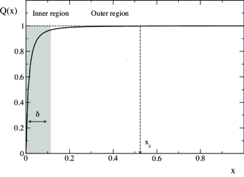
Figure 1: Shape of the order parameter function $Q(x)$ for $T\ll 1$ in the Parisi parameterization. The horizontal arrow shows the extent of the boundary layer of thickness $\delta\sim T$ as $T\to 0$.

From the Figure we see that for very small $T$ the function $Q(x)$ is slowly varying for $\delta\ll x\leq x_{c}$. However, in the boundary layer $0<x\leq\delta$, it undergoes an abrupt and rapid change. In the limit $T\to 0$ the thickness $\delta\sim T\to 0$ and the order parameter function becomes discontinuous at $x=0$.

Uniform approximate solutions valid for $T\ll 1$ can be constructed by using the boundary layer theory, that is by studying the problem separately inside (inner region) and outside (outer region) the boundary layer [23]. One then introduces the notion of the inner and outer limit of the solution. The outer limit is obtained by choosing a fixed $x$ outside the boundary layer, that is in $\delta\ll x\leq 1$, and allowing $T\to 0$. Similarly the inner limit is obtained by taking $T\to 0$ with $x\leq\delta$. This limit is conveniently expressed introducing an inner variable $a$, such as $a=x/\delta$, in terms of which the solution is slowly varying inside the boundary layer as $T\to 0$. The inner and outer solutions are then combined together by matching them in the intermediate limit $x\to 0$, $x/\delta\to\infty$ and $T\to 0$. The inner solution $Q(a)$ is a smooth function of $a$ for $T\to 0$ varying between $0$ and $q_{c}\simeq 1$ [14, 24, 16, 17], similar to $Q(x)$ at finite temperature. In the rest of this paper we shall concentrate on outer solution since as $T\to 0$ it covers the overwhelming part of the interval $[0,1]$.

The behavior of $Q(x)$ for $T\ll 1$ has strong consequences on other relevant quantities, such as, e.g, the four-spin correlation entering into the Hessian matrix. We shall make this more quantitative in the next Sections. Here the only feature we whish to retain is that in the outer region for $T\ll x<x_{c}$ and $T\to 0$, the function $Q(x)$ is driven closer and closer to $Q(x_{c})=q_{c}(T)$ as $T$ approaches zero. It can be shown [25], see also B, that for $T\ll x\leq x_{c}$ and $T\to 0$

$$Q(x)=1-c\,(\beta x)^{-2}+\left(\frac{c}{x_{c}^{2}}-\alpha\right)\,T^{2}+{\cal O}\bigl{(}(\beta x)^{-3},T^{3}\bigr{)},$$ (17)

where $c=0.4108\ldots$ and $\alpha=\lim_{T\to 0}(1-q(x_{c}))/T^{2}$. We note that the breakpoint $x_{c}$ depends on $T$. The dependence is however very weak for low temperatures [22] and the approximation $x_{c}(T)\simeq x_{c}=0.524\ldots$ is rather good for $T\sim 0$. From this expression we see that the variation of $Q(x)$ in the outer region is

$$\frac{Q(x_{c})-Q(x)}{Q(x)}\simeq c\left(\frac{T}{x}\right)^{2}\left[1-\left(\frac{x}{x_{c}}\right)^{2}\right]$$ (18)

so that one can safely take the approximation $Q(x)\sim Q(x_{c})=q_{c}(T)$ as $T\to 0$, the error being ${\cal O}(T^{2})$ at least. Going back to $R$ steps of Replica Symmetry Breaking this approximation translates into

$$Q_{r}\sim Q_{R}=q_{c}(T)=1-\alpha T^{2}+{\cal O}(T^{3}),\qquad T\to 0$$ (19)

for all $r$ in the outer region, that is such that $T\ll x(Q_{r})=p_{r}$ and $T\to 0$, or, equivalently, for fixed $r\not=0$ and $T\to 0$. We shall make this insensitivity with respect to the overlaps $r$ in the $T\ll 1$ limit more precise in the next Sections. Here we just discuss the consequence of the insensitivity on the elements of the Hessian by considering some simple cases.

Suppose the two pairs of replicas are equal: $(a,b)=(c,d)$. In this case from eq. (11) one constructs the simplest Hessian component:

$$M^{ab;ab} = 1-\beta^{2}\Bigl{[}\langle(s^{a}s^{b})^{2}\rangle-\langle s^{a}s^{b}\rangle\langle s^{a}s^{b}\rangle\Bigr{]}$$ (20)

$$= 1-\beta^{2}\Bigl{[}1-\left(Q^{ab}\right)^{2}\Bigr{]}$$

that for the overlap $a\cap b=r$ gives

$$M_{R+1;R+1}^{r;r}=1-\beta^{2}(1-Q_{r}^{2}).$$ (21)

Insensitivity implies that for fixed $r$ and $T\to 0$ we have

$$M_{R+1;R+1}^{r;r}\sim M_{R+1;R+1}^{R;R}=1-2\alpha+{\cal O}(T^{2}),\qquad T\to 0.$$ (22)

Figure 2: Tree configuration for replicas $a,b,c$ with $a\cap b=r$.

The next simple case is when only three replicas are different, in which case we have

$$M^{ab;ac}=-\beta^{2}\Bigl{[}\langle s^{b}s^{c}\rangle-\langle s^{a}s^{b}\rangle\langle s^{a}s^{c}\rangle\Bigr{]},\qquad b\not=c.$$ (23)

Ultrametricity imposes that the three replicas $a,b,c$ with $a\cap b=r$ can be only disposed as shown in Fig. 2. The LA geometries $(a)$ and $(b)$ lead for $T\to 0$ and fixed $r$ and $s$ to

$$M_{R+1}^{r;s}=-\frac{Q_{r}-Q_{r}Q_{s}}{T^{2}}\simeq-\frac{Q_{R}(1-Q_{R})}{T^{2}}=-\alpha+{\cal O}(T^{2}),$$ (24)

while the Replicon geometry $(c)$ yields

$$M_{R+1;s}^{r;r}=-\frac{Q_{s}-Q_{r}^{2}}{T^{2}}\simeq-\frac{Q_{R}(1-Q_{R})}{T^{2}}=-\alpha+{\cal O}(T^{2}).$$ (25)

We shall see below that insensitivity implies that $M_{s}^{r;r}-M_{r}^{r;r}\sim 0$, and that all Replicon components vanish. Then from eq. (15) and (25) it follows

$$M_{R+1}^{R;R}=-\alpha+{\cal O}(T^{2}),\qquad T\to 0.$$ (26)

Similarly from (15) and (22) one obtains

$$2M_{R+1}^{R;R}-M_{R}^{R;R}=1-2\alpha+{\cal O}(T^{2})$$ (27)

which combined with (26) gives

$$M_{R}^{R;R}=-1+{\cal O}(T^{2}),\qquad T\to 0.$$ (28)

The general case with four different replicas cannot be reduced to simple forms and the expression of the four-spin averages is required. This will be derived the next Section.

4 Spin Averages

The evaluation of the Hessian components requires the computation of the four-spin averages $\langle s^{a}s^{b}s^{c}s^{d}\rangle$ for a generic geometry of the four replicas. This can be done by introducing the generating function

$${\cal Z}({\bm{b}})=\exp\bigl{\{}nG_{-1}({\bm{b}})\bigr{\}}={\rm Tr}_{s^{a}}\,\exp\left({\frac{1}{2}\sum_{ab}\Lambda_{ab}\,s^{a}s^{b}+\sum_{a}b_{a}\,s^{a}}\right)$$ (29)

where $\Lambda_{ab}$, equal to $\beta^{2}Q_{ab}$ with $\beta=1/T$ for the SK model, is a generic $n\times n$ symmetric matrix with Parisi’s block structure,

$$\left.\Lambda_{ab}\right|_{a\cap b=r}=\lambda_{r},\qquad r=0,\ldots,R+1.$$ (30)

Spin averages follow from differentiation

$$\langle s^{a}s^{b}\cdots\rangle=\lim_{n\to 0}\frac{1}{{\cal Z}({\bm{b}})}\ \Bigl{[}\frac{\partial}{\partial b_{a}}\left.\frac{\partial}{\partial b_{b}}\cdots\Bigr{]}\ {\cal Z}({\bm{b}})\right|_{b_{1}=\cdots=b_{n}=0}.$$ (31)

Introducing the “block indexes” $a_{k}$,

$$a=(a_{0},a_{1},\ldots,a_{R}),\qquad a_{k}=0,\ldots\frac{p_{k}}{p_{k+1}}-1$$ (32)

where $p_{k}$, with $n=p_{0}>p_{1}>\cdots>p_{R}>p_{R+1}=1$, are the block sizes, the generating function can be written as multiple integrals over independent Gaussian variables:

$${\cal Z}({\bm{b}})=\int{\cal D}_{R}(\alpha)\prod_{0}^{R}\exp G_{R}(b^{R}_{\alpha}+b_{\alpha})$$ (33)

where ${\cal D}_{R}(\alpha)$ is the short-hand notation for:

$$\int{\cal D}_{R}(\alpha) \equiv \prod_{t=0}^{R}\int\prod_{0}^{t-1}Dz^{t}_{\alpha}$$ (34)

$$= \prod_{t=0}^{R}\int\prod_{\alpha_{0},\ldots,\alpha_{t-1}}Dz_{\alpha_{0},\ldots,\alpha_{t-1}}$$

and $z^{t}_{\alpha}=z_{\alpha_{0},\ldots,\alpha_{t-1}}$ are independent Gaussian random variables of zero mean and variance one:

$$Dz\equiv\frac{dz}{\sqrt{2\pi}}e^{-z^{2}/2}.$$ (35)

The function $G_{R}(b)$ is the “free energy” of a single spin in a field $b$:

$$\exp G_{R}(b)={\rm Tr}_{s}\,\exp(b\,s)=2\cosh b.$$ (36)

and the frozen (random) field $b^{R}_{\alpha}$, given by

$$b^{R}_{\alpha}=\sum_{t=0}^{R}\sqrt{\Delta\,\lambda_{t}}\,z^{t}_{\alpha}$$ (37)

where $\Delta\lambda_{t}=\lambda_{t}-\lambda_{t-1}$, keeps track of the contributions from the various blocks.

Inserting the form (33) of ${\cal Z}({\bm{b}})$ into eq. (31), and noticing that differentiation with respect to $b_{a}$ can be replaced by differentiation with respect to $b^{R}_{a}$, we obtain

$$\langle s^{a}s^{b}\cdots\rangle = \lim_{n\to 0}\frac{1}{{\cal Z}(0)}\left[\frac{\partial}{\partial b^{R}_{a}}\frac{\partial}{\partial b^{R}_{b}}\cdots\right]\int{\cal D}_{R}(\alpha)\prod_{0}^{R}\exp G_{R}(b^{R}_{\alpha})$$ (38)

$$= \lim_{n\to 0}\frac{1}{{\cal Z}(0)}\int{\cal D}_{R}(\alpha)\prod_{0}^{R}\exp G_{R}(b^{R}_{\alpha})$$

$$\phantom{======}\times\left[\frac{\partial}{\partial b^{R}_{a}}\,G_{R}(b^{R}_{a})\right]\left[\frac{\partial}{\partial b^{R}_{b}}\,G_{R}(b^{R}_{b})\right]\cdots$$

For any given geometry of the replicas $a,b,c\ldots$ the integrals can now be performed recursively from scale $R$ up to scale $0$. To illustrate the procedure let us consider

$${\cal Z}(0)=\int{\cal D}_{R}(\alpha)\prod_{0}^{R}\exp G_{R}(b^{R}_{\alpha}).$$ (39)

The field $b^{R}_{\alpha}$ can be written as

$$b^{R}_{\alpha} = \sqrt{\Delta\lambda_{R}}\,z^{R}_{\alpha}+\sum_{t=0}^{R-1}\sqrt{\Delta\,\lambda_{t}}\,z^{t}_{\alpha}$$ (40)

$$= \sqrt{\Delta\lambda_{R}}\,z^{R}_{\alpha}+b^{R-1}_{\alpha}.$$

Then splitting out the $z^{R}_{\alpha}$-integrals, and recalling that $z^{R}_{\alpha}$ depends only upon indexes $\alpha_{0},\ldots,\alpha_{R-1}$, one has:

$${\cal Z}(0)=\int{\cal D}_{R-1}(\alpha)\prod_{0}^{R-1}\int Dz^{R}_{\alpha}\exp\left\{p_{R}\,G_{R}(\sqrt{\Delta\lambda_{R}}\,z^{R}_{\alpha}+b^{R-1}_{\alpha})\right\}.$$ (41)

This structure suggests introducing quantities $G_{r}(b)$ as

$$\exp\left\{p_{r}\,G_{r-1}(b^{r-1}_{\alpha})\right\}=\int Dz^{r}_{\alpha}\,\exp\left\{p_{r}\,G_{r}(\sqrt{\Delta\lambda_{r}}\,z^{r}_{\alpha}+b^{r-1}_{\alpha})\right\}$$ (42)

so that eq. (39) can be written as

$${\cal Z}(0)=\int{\cal D}_{R-1}(\alpha)\prod_{0}^{R-1}\exp\left\{p_{R}\,G_{R-1}(b^{R-1}_{\alpha})\right\},$$ (43)

that has the same form of (39) provided $R\to R-1$. The entire process can be iterated up to level $0$ and leads to

$${\cal Z}(0)=\exp\left\{p_{0}G_{-1}(0)\right\}=\int Dz\exp\left\{p_{0}\,G_{0}(\sqrt{\lambda_{0}}\,z)\right\}.$$ (44)

In the limit $p_{0}=n\to 0$ one recovers the usual expression [12]

$$G_{-1}(0)=\int Dz\,G_{0}(\sqrt{\lambda_{0}}\,z).$$ (45)

Equation (42) has an interesting “physical” interpretation. The quantity $G_{R}(b^{R})$ is the free energy of a system of one spin, i.e. of size $1$, in the replica space in presence of the frozen field $b^{R}$, that is with all random (Gaussian) $z^{r}$ held fixed. To move one level up, $R\to R-1$, we have to unfreeze and integrate over $z^{R}$, while keeping all other fields $z^{t}$ with $t<R$ frozen. The fields $z^{t}$ with $t<R$ give the effective action, under the form of a (random) field, of the spins $s^{b}$ on the spin $s^{a}$ with $a\cap b=t<R$. Then integration over the field $z^{R}$ means that only the spins $s^{a}$ and $s^{b}$ such that $a\cap b=R$ are summed in the trace. All others are kept frozen. Thus the quantity $G_{R-1}(b^{R-1})$ can be seen as the free energy (density) of a system in the replica space of size $p_{R}$ in presence of an external field $b^{R-1}$, which gives the interaction with the frozen spins, that is the frozen degrees of freedom. Extension to the successive $z^{r}$-integration is straightforward. The quantity $G_{r-1}(b^{r-1})$ is obtained by integrating out in turn the random fields $z^{t}$ with $t\geq r$, while keeping all $z^{t}$ with $t<r$ frozen. This means that the trace is restricted to spins $s^{a}$ and $s^{b}$ such that $a\cap b=t\geq r$. The contribution from the spins not included into the trace, and hence frozen, is taken into account by the frozen field $b^{r-1}$. The quantity $G_{r-1}(b^{r-1})$ is then the free energy (density) of a system of size $p_{r}$ in the replica space in presence of the external field $b^{r-1}$, which accounts for the degrees of freedom still frozen at scale $r$.

The free energy $G_{-1}(0)$ is part of the total free energy density of the system, see eqs. (6) and (29), and thus it is itself an intensive quantity in the real space. This implies that $p_{r}G_{r-1}$ are intensive quantities, and hence as $n\to 0$ the $p_{r}$ become densities in the real space: $0<p_{r}<1$. The $p_{r}$ give a measure of the density of the frozen degrees of freedom at scale $r-1$ as measured from the overlap. Consider indeed the function

$$x(q)=n+\sum_{r=0}^{R}(p_{r+1}-p_{r})\,\theta(q-Q_{r})$$ (46)

which equals the number of pairs of replicas with overlap $Q^{ab}$ less or equal to $q$: $x(q)=p_{r+1}$ if $Q_{r}<q<Q_{r+1}$. The function $x(q)$ is not decreasing with $q$, thus $p_{r}<p_{r^{\prime}}$ if $r<r^{\prime}$ as $n\to 0$. Indeed in going from level $r$ to level $r-1$ the number of unfrozen degrees of freedom, that is the number of spins in the replica space over which the trace is done, increases, and hence the number of frozen degrees of freedom decreases, as signaled by the decrease of the value of the overlap. This picture is fully consistent with the dynamical formulation of CHS [26, 27] in terms of time-scales and density of frozen/unfrozen degrees of freedom.

We can now turn to the problem of calculating spin averages. This differs from that of ${\cal Z}(0)$ by the presence of terms that depends on the fields $b^{R}_{a}$, cfr. eqs. (38) and (39). The recursion relation (42) is the usual rule to compute the free energy when some frozen degrees of freedom become unfrozen, and hence must be summed up in the trace. In the specific case those frozen at scale $r$ but unfrozen at scale $r-1$, represented by the fields $z^{r}$. The presence of $p_{r}$ instead of $p_{r+1}$ in the integrand follows because at scale $r$ there are $p_{r}/p_{r+1}$ disjoint systems in the replica space, all with the same free energy, that merge at scale $r-1$. This suggests the following recursion relation for the calculation of spin averages. Let $F_{s}(b^{s}_{a})$ be a generic function of the field $b^{s}_{a}$ at scale $s$. We then define the quantity $F_{s-1}(b^{s-1}_{a})$ at scale $s-1$ as the average of $F_{s}(b^{s}_{a})$ over the random field $z^{s}$ weighted with the statistical weight of the state, that is,

$$F_{s-1}(b^{s-1}_{a}) = Z_{s-1}(a)^{-1}$$ (47)

$$\times\int Dz^{s}_{a}\,Z_{s}(a)^{p_{s}/p_{s+1}}\,F_{s}(\sqrt{\Delta\lambda_{s}}\,z^{s}_{a}+b^{s-1}_{a}).$$

where

$$Z_{r}(\alpha)\equiv Z_{r}(b^{r}_{\alpha}) = \exp\bigl{\{}p_{r+1}\,G_{r}(b^{r}_{\alpha})\bigr{\}}$$ (48)

$$= \exp\bigl{\{}p_{r+1}\,G_{r}(\sqrt{\Delta\lambda_{r}}\,z^{r}_{\alpha}+b^{r-1}_{\alpha})\bigr{\}}$$

This recursion relation is supplemented by the boundary condition

$$F_{s}(b^{s}_{a})\Bigr{|}_{s=r}=F_{r}(b^{r}_{a})$$ (49)

where $F_{r}(b_{r})$ is a known expression. Assume for example that

$$F_{r}(b^{r}_{a})=\frac{\partial}{\partial b^{r}_{a}}\,G_{r}(b^{r}_{a})$$ (50)

then a simple calculation shows that

$$F_{r-1}(b^{r-1}_{a})=\frac{\partial}{\partial b^{r-1}_{a}}\,G_{r-1}(b^{r-1}_{a}).$$ (51)

This result is not unexpected since it just states that the magnetization $m_{r}$ at any scale $r$ is given by the derivative of the free energy of that scale with respect to the applied field at that scale:

$$m_{r}(b^{r}_{a})=\frac{\partial}{\partial b^{r}_{a}}\,G_{r}(b^{r}_{a}).$$ (52)

From this result it immediately follows that

$$\langle s^{a}\rangle = m_{-1}(h)=\frac{\partial}{\partial h}G_{-1}(h)$$ (53)

$$= \frac{\partial}{\partial h}\int Dz\,G_{0}(\sqrt{\lambda_{0}}\,z+h)=\int Dz\,m_{0}(\sqrt{\lambda_{0}}\,z+h).$$

where $h$ is an external field. Clearly $\langle s^{a}\rangle=0$ if $h=0$.

Figure 3: $\langle s^{a}s^{b}\rangle_{a\cap b=r}=Q_{r}$ tree configuration.

To compute the two-spin correlation $\langle s^{a}s^{b}\rangle$ with $a\cap b=r$, i.e. the overlap $Q_{r}$, we have to evaluate the integral

$$\langle s^{a}s^{b}\rangle\rightarrow\int{\cal D}_{R}(\alpha)\prod_{0}^{R}Z_{R}(\alpha)\ m_{R}(b^{R}_{a})\,m_{R}(b^{R}_{b})$$ (54)

where we used (52). On a branch-tree diagram the two replicas $a$ and $b$ with $a\cap b=r$ are on different branches for scales $s>r$, see Fig. 3, i.e., they belong to different systems. The two local fields $b^{s}_{a}$ and $b^{s}_{b}$, and hence the magnetizations, are independent from each other and the integration factorizes. Then

$$\langle s^{a}s^{b}\rangle\rightarrow\int{\cal D}_{r}(\alpha)\prod_{0}^{r}Z_{r}(\alpha)\ m_{r}(b^{r}_{a})^{2}$$ (55)

since at scale $r$ the two replicas end up in the same system of size $p_{r}$ and the two fields $b^{r}_{a}$ and $b^{r}_{b}$ become equal. This expression suggests introducing the quantity

$$F_{s}(b^{s}_{a})=m_{r,s}^{(2)}\bigl{(}b^{s}_{a})$$ (56)

with the boundary condition

$$m_{r,r}^{(2)}(b^{r}_{a})=m_{r}(b^{r}_{a})^{2}$$ (57)

in terms of which we have

$$\langle s^{a}s^{b}\rangle\Bigr{|}_{a\cap b=r}=m_{r,-1}^{(2)}(h)\stackrel{{\scriptstyle n\to 0}}{{=}}\int Dz\,m_{r,0}^{(2)}(\sqrt{\lambda_{0}}\,z+h)$$ (58)

where $m_{r,0}^{(2)}$ is computed from the recursion relation (47) with (56) and (57).

For higher order spin correlations we proceed in a similar way. Consider for example the four-spin correlation

Figure 4: Longitudinal-Anomalous Sector tree configuration.

$$\langle s^{a}s^{b}s^{c}s^{d}\rangle^{r,s}_{t}\rightarrow\int{\cal D}_{R}(\alpha)\prod_{0}^{R}Z_{R}(\alpha)\ m_{R}(b^{R}_{a})\,m_{R}(b^{R}_{b})\,m_{R}(b^{R}_{c})\,m_{R}(b^{R}_{d})$$ (59)

where the replicas $a,b,c,d$ have the LA Sector configuration shown in Fig. 4. The four replicas are independent from scale $R$ to $t$, where the replicas $b$ and $c$ end up in the same system in the replica space and the fields $b^{t}_{b}$ and $b^{t}_{c}$ become equal. Thus

$$\langle s^{a}s^{b}s^{c}s^{d}\rangle^{r,s}_{t}\rightarrow\int{\cal D}_{t}(\alpha)\prod_{0}^{t}Z_{t}(\alpha)\ m_{t}(b^{t}_{a})\,m_{t}(b^{t}_{b})^{2}\,m_{t}(b^{t}_{d}).$$ (60)

Moving up along the tree the surviving three replicas remain in different systems up to scale $r$, where the replicas $a$ and $b$ eventually find themselves into the same system. Then, by using the quantity $m_{r,s}^{(2)}$ introduced for the two-spin correlation, we can write

$$\langle s^{a}s^{b}s^{c}s^{d}\rangle^{r,s}_{t}\rightarrow\int{\cal D}_{r}(\alpha)\prod_{0}^{r}Z_{r}(\alpha)\ m_{r}(b^{r}_{a})\,m_{t,r}^{(2)}(b^{r}_{a})\,m_{r}(b^{r}_{d})$$ (61)

where $m_{t,r}^{(2)}(b^{r})$ is obtained from the recursion relation (47) with the initial condition $m_{t,t}^{(2)}(b^{t})=m_{t}(b^{t})^{2}$. For the next step we observe that replicas $a$ and $d$ remain into different subspaces up to scale $s$. Thus by introducing the quantity

$$F_{k}(b^{k}_{a})=m_{t,r,k}^{(2,1)}(b^{k}_{a})$$ (62)

with the boundary condition,

$$m_{t,r,r}^{(2,1)}(b^{r}_{a})=m_{r}(b^{r}_{a})\,m_{t,r}^{(2)}(b^{r}_{a})$$ (63)

we can move up along the tree up to scale $s$, and

$$\langle s^{a}s^{b}s^{c}s^{d}\rangle^{r,s}_{t}\rightarrow\int{\cal D}_{s}(\alpha)\prod_{0}^{s}Z_{s}(\alpha)\ m_{t,r,s}^{(2,1)}(b^{s}_{a})\,m_{s}(b^{s}_{a}).$$ (64)

The last step from scale $s$ to scale $0$ is now straightforward. We introduce the quantity

$$F_{k}(b^{k}_{a})=m_{t,r,s,k}^{(2,1,1)}(b^{k}_{a})$$ (65)

with the boundary condition,

$$m_{t,r,s,s}^{(2,1,1)}l(b^{s}_{a})=m_{t,r,s}^{(2,1)}(b^{s}_{a})\,m_{s}(b^{s}_{a})$$ (66)

so that the final result reads

$$\langle s^{a}s^{b}s^{c}s^{d}\rangle^{r,s}_{t}=m_{t,r,s,-1}^{(2,1,1)}(h)\stackrel{{\scriptstyle n\to 0}}{{=}}\int Dz\,m_{t,r,s,0}^{(2,1,1)}(\sqrt{\lambda_{0}}\,z+h).$$ (67)

In a similar way, once the replica geometry is specified, one can compute spin averages involving any number of spins.

The above results, valid for any finite $R$, are easily extended to the continuous case $R\to\infty$. In this case, since the values of $Q^{ab}$, and hence those of $\lambda_{r}$, are bounded in a finite interval, the differences $\Delta\lambda_{r}\to 0$ as $R\to\infty$ to account for an infinite number of values in a finite interval. As a consequence the recursion relations are replaced by differential equations. In particular the recursion relation (42) becomes the Parisi equation [12], while eq. (47) is replaced by the partial differential equation

$$\dot{F}(x,b)=-\frac{\dot{\lambda}(x)}{2}\Bigl{[}F^{\prime\prime}(x,b)+2\,x\,m(x,b)\,F^{\prime}(x,b)\Bigr{]},\qquad x<t$$ (68)

where $m(x,b)=G^{\prime}(x,b)$, with the initial condition

$$F(x,b)\Bigl{|}_{x=t}=F(t,b)$$ (69)

where $F(t,b)$ is some known expression at scale $t$. As usual the “dot” and the “prime” denote partial derivative with respect to $x$ and $b$, respectively. Details are in A.

We conclude this Section by noticing that this formalisms can be easily extended to calculate the (static) response of the system to external perturbations that act at given scales. Let us denote by $\epsilon^{r}_{a}$ a small external perturbation acting only on scale $r$. We then define the static response as

$$\chi_{r}=\frac{\partial}{\partial\epsilon^{r}_{a}}\langle s^{a}\rangle^{\epsilon^{r}}\Bigr{|}_{\epsilon^{r}=0}$$ (70)

where $\langle s^{a}\rangle^{\epsilon^{r}}$ is the spin average in presence of $\epsilon^{r}$. The perturbation $\epsilon^{r}_{a}$ can be seen as an extra contribution to the frozen field $b^{r}_{a}$. Then, since $\epsilon^{r}_{a}$ acts only on scale $r$, in the recursion relation we end up with $G_{r+1}(\sqrt{\Delta\lambda_{r+1}}z^{r+1}_{a}+b^{r}_{a}+\epsilon^{r}_{a})$. By expanding to the first order in $\epsilon^{r}_{a}$, we finally have

$$\langle s^{a}\rangle^{\epsilon^{r}} \rightarrow \int{\cal D}_{r}(\alpha)\prod_{(\alpha_{0},\ldots,\alpha_{r})\not=(a_{0},\ldots,a_{r})}\int\,Dz^{r+1}_{\alpha}\,\exp\left\{p_{r+1}G_{r+1}(b^{r+1}_{\alpha})\right\}$$ (71)

$$\times\int\,Dz^{r+1}_{a}\exp\left\{p_{r+1}G_{r+1}(b^{r+1}_{a})+p_{r+1}\epsilon^{r}_{a}m_{r+1}(b^{r+1}_{a})\right\}\,m_{r+1}(b^{r+1}_{a})$$

and a similar expression for the normalization ${\cal Z}_{\epsilon^{r}}(0)$. By neglecting all unnecessary indexes, the recursion relation (47) is then replaced by

$$m_{r}^{\epsilon^{r}}(b) = \exp\left\{-p_{r+1}\,G_{r}^{\,\epsilon^{r}}(b)\right\}$$ (72)

$$\times\int Dz\exp\left\{p_{r+1}G_{r+1}(\sqrt{\Delta\lambda_{r+1}}\,z+b)+p_{r+1}\,\epsilon^{r}\,m_{r+1}(\sqrt{\Delta\lambda_{r+1}}\,z+b)\right\}\$$

$$\phantom{xxxxxxxxxxxxxxxxxxxxxxxx}\times m_{r+1}(\sqrt{\Delta\lambda_{r+1}}\,z+b)$$

with

$$\exp\left\{p_{r+1}\,G_{r}^{\,\epsilon^{r}}(b)\right\} = \int Dz\exp\Bigl{\{}p_{r+1}G_{r+1}(\sqrt{\Delta\lambda_{r+1}}\,z+b)$$ (73)

$$\phantom{=============}+p_{r+1}\,\epsilon^{r}\,m_{r+1}(\sqrt{\Delta\lambda_{r+1}}\,z+b)\Bigr{\}}.$$

Taking the derivative with respect to $\epsilon^{r}$, and setting $\epsilon^{r}\to 0$, leads to

$$\frac{\partial}{\partial\epsilon^{r}_{a}}\,m_{r}^{\epsilon^{r}}(b)\Bigr{|}_{\epsilon^{r}=0}=p_{r+1}\left(m_{r+1,r}^{(2)}(b)-m_{r}(b)^{2}\right).$$ (74)

Then from eqs. (70) and (71) we have

$$\chi_{r}=p_{r+1}\,\left(Q_{r+1}-Q_{r}\right).$$ (75)

The derivative of the normalization factor ${\cal Z}_{\epsilon^{r}}(0)$ gives a term proportional to $\langle s^{a}\rangle^{2}$, which vanishes in absence of external field. The expression (75) is the static limit of the modified Fluctuation Dissipation Theorem introduced by CHS [26, 27] in dynamics.

5 Replicon Sector

The Hessian is a $\frac{n(n-1)}{2}\times\frac{n(n-1)}{2}$ symmetric matrix that after block-diagonalization [32, 33] becomes a string of $(R+1)\times(R+1)$ blocks along the diagonal for the LA Sector, followed by $1\times 1$ fully diagonalized blocks, for the Replicon Sector. The diagonal elements in the Replicon Sector are given by:

$$\lambda_{\rm R}(r;\hat{k}\hat{l})=M_{\hat{k};\hat{l}}^{r;r}.$$ (76)

To evaluate $M_{\hat{k};\hat{l}}^{r;r}$ we need the matrix elements $M_{u;v}^{r;r}$, eq. (11), that is the four-spin average $\langle s^{a}s^{b}s^{c}s^{d}\rangle$ for the Replicon Geometry shown in Figure 5.

Figure 5: Replicon Sector tree configuration.

From the results of Section 4 and A this is given, in absence of an applied external field and for $R\to\infty$, by

$$\langle s^{a}s^{b}s^{c}s^{d}\rangle_{u;v}^{r;r}=m_{u,v}^{(2,2)}(0,0).$$ (77)

The function $m_{u,v}^{(2,2)}(x,b)$ is solution of a chain of partial differential equation of the form

$$\dot{F}(x,b)=-\frac{\beta^{2}\dot{Q}(x)}{2}\Bigl{[}F^{\prime\prime}(x,b)+2\,x\,m(x,b)\,F^{\prime}(x,b)\Bigr{]},$$ (78)

where $m(x,b)$ is the local magnetization at scale $x$ in presence of the field $b$.

In our case, starting from the bottom of the tree in Fig. 5, we first have to solve eq. (78) for $F(x,b)=m(x,b)$ and boundary condition

$$F(x,b)\Bigl{|}_{x=1^{-}}=m(1,b)=\tanh b.$$ (79)

The range of $x$ is $u\leq x\leq 1$ for the left branch of the tree, and $v\leq x\leq 1$ for the right branch. To proceed towards scale $0$ we have to solve next eq. (78) for $F(x,b)=m_{t}^{(2)}(x,b)$ and initial condition

$$F(x,b)\Bigl{|}_{x=t}=m_{t}^{(2)}(t,b)=m(t,b)^{2}$$ (80)

where $t=u,v$ depending upon we are on the left or on the right branch of the tree. The range of $x$ is either $r\leq x\leq u$, left branch, or $r\leq x\leq v$, right branch, see Fig. 5.

To accomplish the last step, $0\leq x\leq r$, we finally solve equation (78) for $F(x,b)=m_{u,v}^{(2,2)}(x,b)$ and initial condition

$$F(x,b)\Bigl{|}_{x=r}=m_{u,v}^{(2,2)}(r,b)=m_{u}^{(2)}(r,b)\,m_{v}^{(2)}(r,b).$$ (81)

While these equations are valid for any temperature $T$, we are interested into their solution in the limit $T\to 0$. Following Pankov [25] one can show, see B, that in the outer region $x\gg T$ and $T\to 0$ the solution of the partial differential equation (78) looses its explicit dependence on the scale variable $x$. As a consequence for $R\to\infty$ the matrix element $M_{u;v}^{r,r}$ becomes independent of $u$ and $v$ for all $r$ such that $p_{r}=x(Q_{r})\gg T$ as $T\to 0$, and this in turns implies that $M_{\hat{k};\hat{l}}^{r;r}$ is independent of $k$ and $l$. Thus by exploiting this insensitivity we conclude that for all $r$ in the outer region

$$M_{\hat{k};\hat{l}}^{r;r}=M_{\widehat{r+1};\widehat{r+1}}^{r;r}=O\left(\frac{1}{R^{2}}\right)\stackrel{{\scriptstyle R\to\infty}}{{=}}0.$$ (82)

The second equality follows from a Ward-Takahashi identity [7]. In the inner region the Replicon spectrum maintains its complexity. However its relevance becomes less and less important as $T$ approaches zero, and vanishes in the limit $T\to 0$ when the thickness of the boundary shrinks to zero. The Replicon spectrum, similarly to the order parameter function $Q(x)$, becomes then discontinuous at $x=0$.

6 Longitudinal-Anomalous Sector

The LA Sector corresponds to the $(R+1)\times(R+1)$ diagonal blocks along the diagonal labeled by the index $k=0,\ldots,R+1$. The matrix element in each block turns out to be

$$\leftidx{{}_{\rm LA}}M_{\hat{k}}^{r;s}=\Lambda_{\hat{k}}(r)\,\delta_{r,s}^{\rm Kr}+\frac{1}{4}M_{\hat{k}}^{r;s}\,\delta_{s}^{(k)},\qquad r,s=0,\ldots,R$$ (83)

where $\Lambda_{\hat{k}}(r)$ is a shorthand for

$$\Lambda_{\hat{k}}(r)=\left\{\begin{array}[]{ll}M_{\hat{k};\widehat{r+1}}^{r;r}&k>r+1,\\ \phantom{x}&\phantom{x}\\ M_{\widehat{r+1};\widehat{r+1}}^{r;r}&k\leq r+1,\\ \end{array}\right.$$ (84)

and $\delta_{s}^{(k)}=p_{s}^{(k)}-p_{s+1}^{(k)}$, $k=0,1,\ldots,R+1$, with

$$p_{s}^{(k)}=\left\{\begin{array}[]{ll}p_{s}&s\leq k\\ 2p_{s}&s>k.\end{array}\right.$$ (85)

$M_{\hat{k}}^{r;s}$ is the RFT of the matrix element $M_{t}^{r;s}$ with respect the cross-overlap $t$, that is,

$$M_{\hat{k}}^{r;s}=\sum_{t=k}^{R+1}p_{t}^{(r,s)}\left(M_{t}^{r;s}-M_{t-1}^{r;s}\right)$$ (86)

with , if $r<s$,

$$p_{t}^{(r,s)}=\left\{\begin{array}[]{ll}p_{t}&t\leq r\\ 2p_{t}&r<t\leq s\\ 4p_{t}&r<s<t\end{array}\right.$$ (87)

For finite temperature the matrix elements are different in each block, however for scales $k$ in the outer region the RFT $M_{\hat{k}}^{r;s}$ and $\Lambda_{\hat{k}}(r)$ become insensitive to the value of $k$ as $T\to 0$. All correspondent blocks are then diagonalized through the single eigenvalue equation:

$$\lambda_{\rm LA}f^{r}=M_{\widehat{R+1};\widehat{r+1}}^{r;r}f^{r}+\frac{1}{4}\sum_{s=0}^{R}M_{\widehat{R+1}}^{r;s}\delta_{s}f^{s}$$ (88)

where $\delta_{s}=p_{s}-p_{s+1}$. In the outer region the eigenvectors $f^{r}$ satisfy $f^{r}\not=0$ if $T\ll x(Q_{r})\leq x_{c}$ as $T\to 0$, and zero otherwise. The eigenvalue equation then reduces becomes

$$\lambda_{\rm LA}f^{r}=\frac{1}{4}M_{\widehat{R+1}}^{R;R}\sum_{s=\overline{r}}^{R}\delta_{s}f^{s},\qquad r=\overline{r},\ldots,R.$$ (89)

where $\overline{r}$ is the lower bound of the outer region: $x(Q_{\overline{r}})=\overline{x}\sim\delta$ as $T\to 0$. The diagonal Replicon contribution vanishes for $R\to\infty$, as ensured by the Ward-Takahashi identity, and does not contribute. This equation has two distinct solutions. The first

$$\lambda_{\rm LA}=0$$ (90)

for $\sum_{s=\overline{r}}^{R}\delta_{s}f^{s}=0$, and

$$\lambda_{\rm L} = \frac{1}{4}\left(\sum_{s=\overline{r}}^{R}\delta_{s}\right)\,M_{\widehat{R+1}}^{R;R}$$ (91)

$$= (\overline{x}-1)\bigl{(}1-\beta^{2}\,(1-q_{c}(T)\bigr{)}$$

$$= (\alpha-1)+O(T),\quad T\to 0$$

for $\sum_{s=\overline{r}}^{R}\delta_{s}f^{s}\not=0$. The last equality follows from eq. (19), and $\overline{x}\sim\delta\sim T$ as $T\to 0$. In the inner region, where the LA spectrum maintains the RSB structure, the solutions are smooth functions of the inner variable even for $T\to 0$. For $T\to 0$ the thickness of the boundary layer shrinks to zero, and the eigenvalues (90) and (91) cover the whole LA spectrum, with a discontinuity at $x=0$.

Figure 6: Possible tree configurations corresponding to the Longitudinal-Anomalous Sector with $r<s$ and $t\geq r$.

7 Summary and Conclusions

In this work we have presented the analysis of the very low temperature limit $T\ll 1$ of the spectrum of the Hessian for the Parisi solution of the SK model. It has been long known that in this regime two distinct regions of the interval $x\in[0,1]$ can be identified according to the variation of the order parameter function $Q(x)$ with $x$. We have shown that this has strong consequences on the the structure of the Hessian spectrum. In the first region $x\leq\delta\sim T$, where $Q(x)$ varies rapidly from $Q(0)=0$ up to $Q(\delta)\sim q_{c}(T)\sim 1$, the spectrum maintains the complex structure observed close to the critical temperature $T_{c}$ for the full RSB state. We can call this region the RSB-like regime. In the second region, $T\ll x\leq x_{c}$ with $x_{c}\sim 0.575\ldots$, where $Q(x)$ is slowly varying, the Hessian spectrum has a completely different structure. Here the components of the Hessian matrix become insensitive to changes of the overlaps and the bands observed in the replica symmetry breaking regime collapse. In this region only two distinct eigenvalues survive: a null one and the positive one. This ensures that the Parisi solution of the SK model then remains stable as the temperature goes to zero. Remarkable is the occurrence of zero modes in both the Replicon and the LA Sectors. Null eigenvalues arise from Replicon geometry, with Ward-Takahashi identities protecting them. Note, however, that the zero modes arise also from LA geometry, that is without protection of the Ward-Takahashi identities.

We observe that for $T\ll 1$ the order parameter function is almost constant for $T\ll x\leq x_{c}$, the variation being indeed of order $[Q(x_{c})-Q(x)]/Q(x)={\cal O}\left((T/x)^{2}\right)$. Thus in this region we have a marginally stable (almost) replica symmetric solution, that becomes a genuine replica symmetric solution in the limit $T\to 0$, with self-averaging trivially restored. It is worth to remind that the stability analysis of the replica symmetric solution also leads to two eigenvalues, one of which is zero to the lowest order in $T_{c}-T$ (and negative to higher order), and the other positive.

In the limit $T\to 0$ the region where the RSB structure of the solution is found shrinks to zero, and only the RS part survives. This feature, in a sense, brings about some perfume of conciliation between aspects of Parisi mean-field approach and of the droplet approach [28, 29]. We stress, however, that in order to identify a genuine droplet behavior, corrections to the mean-field have to be studied in more details.

Concerning the multiplicity of the eigenvalues we observe that in each Sector, Replicon and LA, one has to separate the contribution from the RSB-like and the droplet-like regions. The former is proportional to the width $\delta$ of the region. Therefore in the limit $T\to 0$ the contribution from the RSB-like region vanishes, and one has the usual Replicon and LA multiplicities for the droplet-like region.

Finally, we have developed a method to compute spin averages in replica space involving any number of replicas, both for a finite number $R$ of replica symmetry breaking steps and for the continuous limit $R\to\infty$. This generalizes some special cases known for the continuous limit $R\to\infty$, and to our knowledge it is new. Moreover it sheds light on the interpretation of the replica symmetry breaking method and its relation with the dynamical approach. For example we were able to compute the static susceptibility and show that it equals the static limit of the dynamic susceptibility computed via the modified Fluctuation Dissipation Theorem.

Appendix A Spin Averages: continuous case

The expressions derived in Section 4 are valid for any finite number $R$ of replica symmetry breaking steps. Here we shall address the limit $R\to\infty$, where the replica symmetry breaking become continuous. If the values of $\lambda_{r}$ are bounded in a finite interval, as is the case of the SK model, in the limit $R\to\infty$ they must be dense and

$$\Delta\lambda_{r}\to 0\ \mbox{\rm as}\ R\to\infty,\qquad r=0,1,\ldots,R.$$ (92)

so that the integral in the recursion relations can then be evaluated by expanding in powers of $\Delta\lambda_{r}$. We observe that a finite number of “jumps”, that is values of $r$ where $\Delta\lambda_{r}$ remains finite as $R\to\infty$, are possible. One then gets mixed continuous-discrete phase described by a piecewise order parameter function, as those observed, e.g., in spherical $p$ spin-glass models [30, 31]. We shall not discuss this case here.

Let us first consider the recursion relation for the free energy $G_{r}$. In the following we drop all unnecessary indexes. By expanding $G_{r}(\sqrt{\Delta\lambda_{r}}\,z+b)$ in eq. (42) in powers of $\Delta\lambda_{r}$ and integrating over the Gaussian variable $z$, a straightforward algebra leads to

$$G_{r-1}(b)=G_{r}(b)+\frac{\Delta\lambda_{r}}{2}\left[G_{r}^{\prime\prime}(b)+p_{r}\bigl{(}G_{r}^{\prime}(b)\bigr{)}^{2}\right]+O(\Delta\lambda_{r}^{2})$$ (93)

where the “prime” denote differentiation with respect the argument, i.e. the field $b$:

$$G_{r}^{\prime}(b)=\frac{\partial}{\partial b}G_{r}(b).$$ (94)

Next we observe that $G_{r}(b)$ is a function of $p_{r}$, thus to extract the non-trivial part of eq. (93) as $\Delta\lambda_{r}\to 0$ we have to specify what happens to $p_{r}-p_{r-1}$ as $R\to\infty$.

Suppose $p_{r}-p_{r-1}$ does not vanish in the limit $R\to\infty$. In this case eq. (93) implies that

$$G_{r-1}(b)=G_{r}(b)\qquad\mbox{as}\ \Delta\lambda_{r}\to 0\ \mbox{but}\ p_{r}-p_{r-1}\not=0$$ (95)

that is, $G_{r}(b)$ does not depend on the scale. This is what happens, for example, in the SK model for $x_{c}<r<1$, the so called “plateau”. If $p_{r}-p_{r-1}\to 0$ as $\Delta\lambda_{r}\to 0$ then, by defining

$$p_{r}\equiv x\qquad\Rightarrow\qquad p_{r}-p_{r-1}=\Delta x$$ (96)

and changing the notation to $G_{r}(b)=G(x,b)$, equation (93) leads for $\Delta\lambda_{r}\to 0$ to the Parisi equation [12, 36]

$$\dot{G}(x,b)=-\frac{\dot{\lambda}(x)}{2}\left[G^{\prime\prime}(x,b)+x\bigl{(}G^{\prime}(x,b)\bigr{)}^{2}\right]$$ (97)

where the “dot” denotes the (left) derivative with respect to the scale $x$, e.g.,

$$\dot{G}(x,b)=\frac{\partial}{\partial x}G(x,b)\equiv\lim_{\Delta x\to 0}\frac{G(x,b)-G(x-\Delta x,b)}{\Delta x}.$$ (98)

We note that with this definition the validity of the partial differential equation (97) can be extended to include the case (95) since the derivative is always well defined. As a consequence the initial condition simply reads, see eq. (36),

$$G(x=1^{-},b)=\ln\bigl{(}2\,\cosh b\bigr{)}$$ (99)

while (45) becomes

$$G_{-1}(b)=\int Dz\,G(0,\sqrt{\lambda(0)}\,z+b).$$ (100)

For the recursion relation (47) we follows a similar procedure, that is we expand the r.h.s. of (47) in powers of $\Delta\lambda_{r}$ and integrate over the Gaussian variable $z$. This leads to

$$F_{r-1}(b)=F_{r}(b)+\frac{\Delta\lambda_{r}}{2}\Bigl{[}F_{r}^{\prime\prime}(b)+2p_{r}G_{r}^{\prime}(b)F_{r}^{\prime}(b)\Bigr{]}+O(\Delta\lambda_{r}^{2}).$$ (101)

As before if $p_{r}-p_{r-1}$ does not vanish as $\Delta\lambda_{r}\to 0$, the recursion relation reduces to

$$F_{r-1}(b)=F_{r}(b).$$ (102)

If, however, $p_{r}-p_{r-1}=\Delta x\to 0$ as $\Delta\lambda_{r}\to 0$ we end up with the partial differential equation

$$\dot{F}(x,b)=-\frac{\dot{\lambda}(x)}{2}\Bigl{[}F^{\prime\prime}(x,b)+2\,x\,m(x,b)\,F^{\prime}(x,b)\Bigr{]},\qquad x<t$$ (103)

where $m(x,b)=G^{\prime}(x,b)$ is the magnetization at scale $x$ in presence of a field $b$, with the initial condition

$$F(x,b)\Bigl{|}_{x=t}=F(t,b)$$ (104)

where $F(t,b)$ is a known expression at scale $t$.

As an example consider the two-spin correlation $\langle s^{a}s^{b}\rangle$ with $a\cap b=r$. From eq. (58) it readily follows that

$$\langle s^{a}s^{b}\rangle\Bigr{|}_{a\cap b=r}=\int Dz\,m_{r}^{(2)}(0,\sqrt{\lambda(0)}\,z+h)$$ (105)

where $m_{r}^{(2)}(x,b)$ is solution of the the partial differential equation

$$\dot{m}_{r}^{(2)}(x,b)=-\frac{\dot{\lambda}(x)}{2}\Bigl{[}{m_{r}^{(2)}}^{\prime\prime}(x,b)+2\,x\,m(x,b)\,{m_{r}^{(2)}}^{\prime}(x,b)\Bigr{]}$$ (106)

for $0<x<r$ and initial condition

$$m_{r}^{(2)}(x=r,b)=m(r,b)^{2}.$$ (107)

To our knowledge this equation was first derived by Goltsev [37].

For the four-spin correlation $\langle s^{a}s^{b}s^{c}s^{d}\rangle^{r,s}_{t}$ of Fig. 4 we have a similar expression:

$$\langle s^{a}s^{b}s^{c}s^{d}\rangle^{r,s}_{t}=\int Dz\,m_{t,r,s}^{(2,1,1)}(0,\sqrt{\lambda(0)}\,z+h)$$ (108)

where $m_{t,r,s}^{(2,1,1)}(x,b)$ is solution of the partial differential equation

$$\dot{m}_{t,r,s}^{(2,1,1)}(x,b)=-\frac{\dot{\lambda}(x)}{2}\Bigl{[}{m_{t,r,s}^{(2,1,1)}}^{\prime\prime}(x,b)+2\,x\,m(x,b)\,{m_{t,r,s}^{(2,1,1)}}^{\prime}(x,b)\Bigr{]}$$ (109)

for $0<x<s$ and initial condition

$$m_{t,r,s}^{(2,1,1)}(x=s,b)=m_{t,r}^{(2,1)}(s,b)\,m(s,b).$$ (110)

The function $m_{t,r}^{(2,1)}(x,b)$ is itself solution of the partial differential equation

$$\dot{m}_{t,r}^{(2,1)}(x,b)=-\frac{\dot{\lambda}(x)}{2}\Bigl{[}{m_{t,r}^{(2,1)}}^{\prime\prime}(x,b)+2\,x\,m(x,b)\,{m_{t,r}^{(2,1)}}^{\prime}(x,b)\Bigr{]}$$ (111)

for $s<x<r$ and initial condition

$$m_{t,r}^{(2,1)}(x=r,b)=m_{t}^{(2)}(r,b)\,m(r,b).$$ (112)

Finally $m_{t}^{(2)}(x,b)$ is solution of equation (106) for $r<x<t$ and initial condition $m_{t}^{(2)}(x=t,b)=m(t,b)^{2}$.

We conclude this Section by noticing that if we take $F(x,b)=m(x,b)$, then the differential equation (103) becomes the known differential equation[14],

$$\dot{m}(x,b)=-\frac{\dot{\lambda}(x)}{2}\Bigl{[}m^{\prime\prime}(x,b)+2\,x\,m(x,b)\,m^{\prime}(x,b)\Bigr{]}$$ (113)

with the initial condition

$$m(1^{-},b)=\tanh b$$ (114)

derived by Sommers and Dupont for the local magnetization. Numerical solution of these equations can be found by using, e.g., the method described in Ref. [22].

Appendix B The Pankov scaling regime

To discuss the Pankov regime $T\to 0$ and $T\ll x\ll 1$ we first perform the change of variable $b=\beta y$ into the partial differential equation (103) to make explicit the temperature dependence. In the new variable the equation reads

$$\dot{F}(x,y)=-\frac{\dot{\lambda}(x)}{2\beta^{2}}\Bigl{[}F^{\prime\prime}(x,y)+2\beta x\,m(x,y)\,F^{\prime}(x,y)\Bigr{]}$$ (115)

where the “prime” now denotes differentiation with respect to $y$, and the local magnetization is $m(x,y)=\beta^{-1}\,G^{\prime}(x,y)$, see footnote page 3. Following Pankov [25] we assume that the dependence on the local fields $y$ is via the combination $z=\beta xy$, that is,

$$F(x,y)=\widetilde{F}(x,z),\qquad z=\beta xy$$ (116)

and similarly for $m(x,y)$. The differential equation (115) then becomes

$$x\,\dot{\widetilde{F}}(x,z) = -\frac{x^{3}\,\dot{\lambda}(x)}{2}\Bigl{[}\widetilde{F}^{\prime\prime}(x,z)+2\widetilde{m}(x,z)\,\widetilde{F}^{\prime}(x,z)\Bigr{]}$$ (117)

$$\phantom{===}-z\widetilde{F}^{\prime}(x,z).$$

Pankov has shown that in the outer region the “tilded” functions do not depend explicitly on the scale variable $x$: $\widetilde{F}(x,z)=\widetilde{F}(z)$. All dependence on scale, field and temperature enters via the combination $\beta xy$. Pankov called this the scaling regime.

From eq. (117) it is clear that the Pankov scaling regime is only possible iff

$$\frac{x^{3}\,\dot{\lambda}(x)}{2}=c=\mbox{\rm constant}\quad\Rightarrow\quad\lambda(x)=\mbox{\sl const.}-\frac{c}{x^{2}}$$ (118)

in which case the partial differential equation (117) reduces to the ordinary second order differential equation

$$\widetilde{F}^{\prime\prime}(z)=-\left[\frac{z}{c}+2\,\widetilde{m}(z)\right]\,\widetilde{F}^{\prime}(z).$$ (119)

In the SK model $\lambda(x)=\beta^{2}\,Q(x)$, where $Q(x)$ is the order parameter function, then from (118) it follows that in the outer region $Q(x)$ has the form

$$Q(x)=\mbox{\sl const.}-\frac{c}{(\beta x)^{2}}.$$ (120)

Equation (17) now follows by imposing $Q(x_{c})=q_{c}(T)=1-\alpha T^{2}+{\cal O}(T^{3})$.

Appendix C Descending the replica tree: the frozen field probability distribution functions

In Section 4 we have shown how spin averages can be computed using a bottom-up approach, that is starting from level $R$ at the bottom of the tree and climbing up towards level $0$ at the top of the tree. A top-down approach is also possible.

To illustrate the procedure suppose we have to compute the following average,

$$\langle g\rangle=\frac{\int{\cal D}_{r}(\alpha)\prod_{0}^{r}Z_{r}(\alpha)\ g_{r}(b^{r}_{a})}{\int{\cal D}_{r}(\alpha)\prod_{0}^{r}Z_{r}(\alpha)}$$ (121)

where $g_{r}(b^{r}_{a})$ is a generic function of the frozen field $b^{r}_{a}$ at scale $r$. For example $g_{r}(b^{r}_{a})=m_{r}(b^{r}_{a})^{2}$ for the two-spin correlation, see eq. (55). The average (121) can be rewritten in the simple form

$$\langle g\rangle=\int dy\,P_{r}(y)\,g_{r}(y).$$ (122)

by introducing the frozen field probability distribution function at scale $r$

$$P_{r}(y)=\frac{\int{\cal D}_{r}(\alpha)\prod_{0}^{r}Z_{r}(\alpha)\ \delta(b^{r}_{a}-y)}{\int{\cal D}_{r}(\alpha)\prod_{0}^{r}Z_{r}(\alpha)}=\langle\delta(b^{r}_{a}-y)\rangle.$$ (123)

Following the procedure outlined in Section 4 we can integrate the Gaussian variables $z^{r}_{\alpha}$ in eq. (123), ending with

$$P_{r}(y)=\frac{\int{\cal D}_{r-1}(\alpha)\prod_{0}^{r-1}Z_{r-1}(\alpha)\ g_{r-1}(b^{r-1}_{a};y)}{\int{\cal D}_{r-1}(\alpha)\prod_{0}^{r-1}Z_{r-1}(\alpha)}$$ (124)

where

$$g_{r-1}(b;y)=\frac{1}{\sqrt{2\pi\Delta\lambda_{r}}}\exp\left\{-\frac{(y-b)^{2}}{2\Delta\lambda_{r}}+p_{r}\,\bigl{[}G_{r}(y)-G_{r-1}(b)\bigr{]}\right\}.$$ (125)

Equation (124) has the same structure as eq. (121), thus we can write

$$P_{r}(y)=\int dy^{\prime}P_{r-1}(y^{\prime})\ g_{r-1}(y^{\prime};y)$$ (126)

where $P_{r-1}(y)$ is given by eq. (123) with $r\to r-1$. Inserting the expression (125) into (126) leads to the recursion relation

$$P_{r}(y) = \int Dz\exp\left\{p_{r}\,\bigl{[}G_{r}(y)-G_{r-1}(\sqrt{\Delta\lambda_{r}}\,z+y)\bigr{]}\right\}$$ (127)

$$\phantom{================}\times P_{r-1}(\sqrt{\Delta\lambda_{r}}\,z+y)$$

that gives the frozen field distribution at scale $r$ one it is known at scale $r-1$. The initial condition is specified at level $0$, at the top of the tree, and reads

$$P_{0}(y)=\frac{1}{\sqrt{2\pi\lambda_{0}}}\exp\left\{-\frac{(y-b)^{2}}{2\lambda_{0}}\right\}.$$ (128)

as follows from eqs. (124) and (125).

In the limit $R\to\infty$ $P_{r}(y)\to P(x,y)$ and the recursion relation (127) is replaced by the partial differential equation

$$\dot{P}(x,y)=\frac{\dot{\lambda}(x)}{2}\Bigl{[}P^{\prime\prime}(x,y)-2\,x\,\bigl{[}m(x,y)\,P(x,y)\bigr{]}^{\prime}\Bigr{]}$$ (129)

where $m(x,y)=G^{\prime}(x,y)$, with the initial condition at $x=0$:

$$P(0,y)=\frac{1}{\sqrt{2\pi\lambda(0)}}\exp\left\{-\frac{(y-b)^{2}}{2\lambda(0)}\right\}.$$ (130)

Equations (129) and (130) where first derived by Sommers and Dupont [14] using a variational approach. We note that taking $g_{r}(b)=m_{r}(b)^{2}$ from eq. (122) one recovers in limit $R\to\infty$ the Sommers-Dupont expression

$$Q(x)=\int dy\,P(x,y)\,m(x,y)^{2}.$$ (131)

The approach in terms of frozen field distribution functions can be generalized to deal with averages of quantities that depend on more then one local field. Suppose for example that $g_{r}\to g_{r}(b^{r}_{a},b^{r}_{b})$ with $a\not=b$. In this case eq. (122) is replaced by

$$\langle g\rangle=\int dy_{1}\,dy_{2}\,P_{r}(y_{1},y_{2})\,g_{r}(y_{1},y_{2})$$ (132)

where $P_{r}(y_{1},y_{2})$ is the probability distribution function of the frozen fields $y_{1}$ and $y_{2}$ lying on two different branches of the tree at scale $r$. This satisfies the top-down recursion relation

$$P_{r}(y_{1},y_{2}) = \int Dz_{1}\,Dz_{2}\prod_{k=1,2}\exp\left\{p_{r}\,\bigl{[}G_{r}(y_{k})-G_{r-1}(\sqrt{\Delta\lambda_{r}}\,z_{k}+y_{k})\bigr{]}\right\}$$ (133)

$$\phantom{============}\times P_{r-1}(\sqrt{\Delta\lambda_{r}}\,z_{1}+y_{1},\sqrt{\Delta\lambda_{r}}\,z_{2}+y_{2}).$$

The initial condition is specified at the branching point $s<r$ where the two branches meet, and reads

$$P_{r}(y_{1},y_{2})\Bigr{|}_{r=s}=\delta(y_{1}-y_{2})\,P_{s}(y_{1}).$$ (134)

It is easy to verify that the frozen field distribution functions obey the sum-rule

$$\int dy_{2}\,P_{r}(y_{1},y_{2})=P_{r}(y_{1}),\qquad\forall r.$$ (135)

In the continuous limit the recursion relation (133) is replaced by the partial differential equation

$$\dot{P}(x,y_{1},y_{2})=\frac{\dot{\lambda}(x)}{2}\sum_{k=1,2}\Bigl{\{}\partial_{k}^{2}P(x,y_{1},y_{2})-2\,x\,\partial_{k}\bigl{[}m(x,y_{k})\,\partial_{k}P(x,y_{1},y_{2})\bigr{]}\Bigr{\}}$$ (136)

where $\partial_{k}=(\partial/\partial y_{k})$. The generalization to frozen field distribution functions of any number of independent frozen fields is straightforward.

References

References

[1]
D. Sherrington and S. Kirkpatrick 1975
Phys. Rev. Lett.35 1792
[2]
G. Parisi 1979
Phys. Rev. Lett.43 1754
[3]
G. Parisi 1980
J. Phys. A 13 1101
[4]
G. Parisi 1980
J. Phys. A 13 1887
[5]
J.R.L. de Almeida and D.J. Thouless 1978
J. Phys. A 11 983
[6]
C. De Dominicis and I. Kondor 1983
Phys. Rev. B 27 606
[7]
C. De Dominicis, T. Temesvari and I. Kondor 1998
J. de Physique IV France8 13
(Preprint cont-mat/9802166)
Equation numbering having been messed up at the editing stage,
the reader should rather consult the cond-mat version.
[8]
A. Crisanti and C. De Dominicis 2010
J. Phys. A 43 055002
[9]
A. Crisanti, C. De Dominicis and T. Sarlat 2010
Eur. Phys. J. B 71 139
[10]
S. F. Edwards and P. W. Anderson 1975
J. Phys. F 5 965
[11]
A. Bray and M. Moore 1979
J. Phys. C 12 79
[12]
G. Parisi 1980
J. Phys. A 13 L115.
[13]
H. Sompolinsky 1981
Phys. Rev. Lett.47 935
[14]
H. J. Sommers and W. Dupont 1984
J. Phys. C 17 5785
[15]
R. Oppermann, M.J. Schmidt and D. Sherrington 2007
Phys. Rev. Lett.98 127201
[16]
M.J. Schmidt and R. Oppermann 2008
Phys. Rev. E 77 061104
[17]
R. Oppermann and M.J. Schmidt 2008
Phys. Rev. E 78 061124
[19]
C. De Dominicis, M. Gabay and B Duplantier,
J. Phys. A: Math. Gen. 15, L47 (1982)
[20]
C. De Dominicis, I. Kondor and T. Temesvari 1998
in Spin Glasses and Random Fields,
A.P. Young Editor (World Scientific), p. 119
[21]
H.-J. Sommers 1985
J. Phys. (France) Lett.46 L-779
[22]
A. Crisanti and T. Rizzo 2002
Phys. Rev. E 65 046137
[23]
see, e.g., C. Bender and S.A. Orszag
Advanced Mathematical Methods For Scientists and Engineers
(Springer, 1999)
[24]
R. Oppermann and D. Sherrington 2005
Phys. Rev. Lett.95 197203
[25]
S. Pankov 2006
Phys. Rev. Lett.96 197204
[26]
A. Crisanti, H. Hörner and H.-J. Sommers 1993
Z. Phys. B 92 257
[27]
A. Crisanti and L. Leuzzi 2007
Phys. Rev. B 75 144301
[28]
T. Aspelmeier, M.A. Moore and A.P. Young 2003
Phys. Rev. Lett.90 127202
see also cond-mat/0209290v1
[29]
A. Crisanti and C. De Dominicis 2010
Europhys. Lett.92 17003
[30]
A. Crisanti and L. Leuzzi 2006
Phys. Rev. B 73 134431
[31]
A. Crisanti and L. Leuzzi 2007
Phys. Rev. B 76 184417
[32]
C. De Dominicis, D.M. Carlucci and T. Temesvari 1997
J. Phys. I France7 105
[33]
T. Temesvari, C. De Dominicis and I. Kondor 1994
J. Phys. A 27 7569
[34]
A. Bray and M. Moore,
in Heidelberg Colloquium on Glassy dynamics and optimizations,
L. Van Hemmen and I. Morgensten Eds.
(Springer-Verlag, 1986).
[35]
A. Crisanti and C. De Dominicis, work in progress.