Simple foreground cleaning algorithm for detecting primordial $B$-mode polarization of the cosmic microwave background

Abstract

We reconsider the pixel-based, “template” polarized foreground removal method within the context of a next-generation, low-noise, low-resolution (0.5 degree FWHM) space-borne experiment measuring the cosmological $B$-mode polarization signal in the cosmic microwave background (CMB). This method was first applied to polarized data by the Wilkinson Microwave Anisotropy Probe (WMAP) team and further studied by Efstathiou et al. We need at least 3 frequency channels: one is used for extracting the CMB signal, whereas the other two are used to estimate the spatial distribution of the polarized dust and synchrotron emission. No extra data from non-CMB experiments or models are used. We extract the tensor-to-scalar ratio ($r$) from simulated sky maps outside the standard polarization mask (P06) of WMAP consisting of CMB, noise ($2~{}\mu$K arcmin), and a foreground model, and find that, even for the simplest 3-frequency configuration with 60, 100, and 240 GHz, the residual bias in $r$ is as small as $\Delta r\approx 0.002$. This bias is dominated by the residual synchrotron emission due to spatial variations of the synchrotron spectral index. With an extended mask with $f_{sky}=0.5$, the bias is reduced further down to $<0.001$.

1. Introduction

Why study the $B$-mode polarization of the cosmic microwave background (CMB)? Detection of the primordial gravitational waves generated during inflation would give us a direct insight into the physical condition of the universe when the energy scale was close to the grand unification scale, $\sim 10^{16}$ GeV (see Liddle & Lyth, 2009, for a recent review and references therein). While a direct detection of the primordial gravitational waves using, e.g., laser interferometers, seems not possible with the present-day technology, an indirect detection using the $B$-mode polarization of the CMB (Seljak & Zaldarriaga, 1997; Kamionkowski et al., 1997) may be possible in the near future (most optimistically, within a few years), provided that the energy scale of inflation at which the observed gravitational waves were generated was indeed as high as the grand unification scale.

We often characterize the amplitude of gravitational waves (also known as tensor perturbations) using the so-called “tensor-to-scalar ratio,” which is conventionally defined as

$$r\equiv\frac{2\langle|h^{+}_{{\mathbf{k}}}|^{2}+|h^{\times}_{{\mathbf{k}}}|^{2}\rangle}{\langle|{\cal R}_{\mathbf{k}}|^{2}\rangle},$$ (1)

where $h^{+}_{\mathbf{k}}$ and $h^{\times}_{\mathbf{k}}$ are the Fourier transform of the amplitudes of two linear polarization states of gravitational waves, and ${\cal R}_{\mathbf{k}}$ is the primordial curvature perturbation, which is a scalar perturbation (hence the name, “tensor-to-scalar ratio”). It is ${\cal R}_{\mathbf{k}}$ that seeded the observed structure in the universe, as well as the dominant component of the observed CMB temperature anisotropy (see Weinberg, 2008, for a recent review and references therein).

The dominant, scalar part of the temperature anisotropy generates radial and tangential polarization patterns around hot and cold spots (Coulson et al., 1994). This is called the $E$-mode polarization, and has been detected with high statistical significance (Brown et al., 2009; Chiang et al., 2010; Larson et al., 2010; Komatsu et al., 2010; QUIET, 2010). However, the $B$-mode polarization, which cannot be generated by the scalar perturbations but can be generated by the tensor perturbations, has not been found yet. The current 95% upper limit on the tensor-to-scalar ratio is $r<0.24$, which mainly comes from the upper limit on the tensor contribution to the temperature anisotropy on large angular scales (Komatsu et al., 2010).

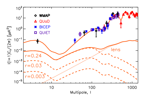
Figure 1.— $E$-mode and $B$-mode polarization power spectra. The diamonds, triangles, stars, and squares show the WMAP seven-year data (Larson et al., 2010), the QUaD final data (Brown et al., 2009), the BICEP two-year data (Chiang et al., 2010), and the QUIET 43 GHz data (QUIET, 2010), respectively. The upper solid line shows the scalar $E$-mode power spectrum of the WMAP seven-year best-fit model. The dashed lines show the primordial $B$-mode power spectra with the tensor-to-scalar ratio of $r=0.24$, which corresponds to the current 95% upper limit (Komatsu et al., 2010), as well as of $r=0.03$ and 0.003. These lines are linearly proportional to $r$. The dotted line shows the secondary $B$-mode power spectrum expected to be generated by the weak gravitational lensing effect converting $E$ modes to $B$ modes (Zaldarriaga & Seljak, 1998). This line is fixed (by the WMAP seven-year best-fit model) and acts as noise for the primordial $B$-mode detection. The lensing contribution becomes comparable to the primordial bump at $l=10$ and 100 for $r=0.003$ and 0.03, respectively.

Given the upper limit on $r$, one can calculate the expected level of the $B$-mode power spectrum (see Figure 1). For $r=0.24$, the $B$-mode power spectrum is smaller than the $E$-mode power spectrum by a factor of 10 at the first bump (created by electrons at $z\lesssim 10$). At the second bump (created by electrons at $z\simeq 1090$), the $B$-mode power spectrum is smaller than the $E$-mode power spectrum by a factor of 50. It is the smallness of the $B$-mode power spectrum that makes the detection of this signal challenging.

There are three sources of noise for $B$-mode detection: (1) Detector noise; (2) Galactic foreground emission; and (3) Gravitational lensing. In this paper, we shall focus on the Galactic foreground. We use a map-based method for reducing the Galactic foreground, and study how the residual foreground limits a measurement of the primordial $B$-mode polarization. The foreground reduction technique we use is motivated by the “template cleaning method” used by the WMAP team (Page et al., 2007; Gold et al., 2009, 2010). This method was further investigated by Efstathiou et al. (2009) in the context of the Planck mission. We shall study this technique in the context of a next-generation, low-noise, low-resolution (0.5 degree FWHM) space-borne experiment.

There is a large body of literature on the issue of polarized foreground cleaning for the $B$-mode detection. Our method is one specific (and relatively simpler) example. For the other methods in the literature, see review articles (Dunkley et al., 2009; Fraisse et al., 2008) and references therein.

This paper is organized as follows. In Section 2, we show how the detector noise and the lensing noise influence the statistical errors on $r$. In Section 3, we describe our method for estimating $r$ in the presence of the Galactic foreground and the dominant scalar $E$-mode polarization. In Section 4, we describe our simulation including CMB, detector noise, and foreground. In Section 5, we present the main results of this paper. We conclude in Section 6.

2. Detector noise and lensing noise

Before we study the effect of the foreground, we show how the detector noise and the lensing noise influence our ability to detect $r$. The detector noise enters into the likelihood of $r$ via the noise power spectrum, $N_{l}^{BB}$. Assuming white noise, we write the noise power spectrum as

$$N_{l}^{BB}=\left(\frac{\pi}{10800}\frac{{w}_{p}^{-1/2}}{{\mu{\rm K}}~{}\rm arcmin}\right)^{2}\mu{\rm K}^{2}~{}{\rm str},$$ (2)

where ${w}_{p}^{-1/2}$ is the noise in Stokes parameters $Q$ or $U$ per pixel whose solid angle, $\Omega_{\rm pix}$, gives $\sqrt{\Omega_{\rm pix}}=1$ arcmin. This quantity is useful because one can compare various experiments on the same scale.

Current and future experiments use many (of order $10^{3}-10^{4}$) detectors to reduce the noise equivalent temperature (NET) down to a few $\mu$K arcmin level. Is this sufficient for detecting primordial $B$ modes? For comparison, the expected sensitivity of Planck combining 70, 100, and 143 GHz is ${w}_{p}^{-1/2}=63~{}{\mu}$K arcmin (see, e.g., Appendix A of Zaldarriaga et al., 2008; Planck Blue Book, 2005).

In Figure 2, we compare the noise power spectra for $w_{p}^{-1/2}=2$ and 10 $\mu$K arcmin to the primordial and lensing $B$ modes. For $r=10^{-3}$ and the 10 $\mu$K arcmin noise, only a few modes ($l=2$, 3, and 4) are above noise. For the 2 $\mu$K arcmin noise, the noise power spectrum is below the lensing $B$-mode power spectrum, and thus noise is no longer the limiting factor (unless we “de-lens” maps and remove the lensing noise). How would this influence our ability to detect $r$?

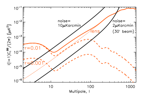
Figure 2.— $B$-mode polarization signal and noise power spectra. The dashed lines show the primordial $B$-mode power spectra with the tensor-to-scalar ratio of $r=0.01$ and 0.001, while the dotted line shows the secondary $B$-mode power spectrum from gravitational lensing. We also show the noise power spectra (Equation (2)) for $w_{p}^{-1/2}=2$ and 10 $\mu$K arcmin with a Gaussian beam window function of $\theta_{\rm FWHM}=30$ arcmin, i.e., $N_{l}^{BB}e^{l^{2}\theta_{\rm FWHM}^{2}/(8\ln 2)}$.

To see this, let us calculate the likelihood of $r$ for a given noise level. For simplicity, we assume that we cover the full sky and the noise per pixel is homogeneous. Then, one can write down the probability distribution function of the measured $B$-mode power spectrum, $\hat{C}_{l}^{BB}$, for a given value of $r$ as (e.g., Equation (8) of Hamimeche & Lewis, 2008)

$$-2\ln P(\hat{C}^{BB}_{l}|r)$$ (3)

$$= (2l+1)\left[\frac{\hat{C}^{BB}_{l}}{rc_{l}^{GW}+c_{l}^{L}+N_{l}^{BB}}+\ln(rc_{l}^{GW}+c_{l}^{L}+N_{l}^{BB})\right.$$

$$\left.\qquad\qquad-\frac{2l-1}{2l+1}\ln(\hat{C}_{l}^{BB})\right],$$

where $c_{l}^{GW}$ is the primordial $B$-mode power spectrum from gravitational waves with $r=1$, and $c_{l}^{L}$ is the secondary $B$ mode from gravitational lensing. We then use Bayes’ theorem to calculate the likelihood for $r$ as ${\cal L}(r|\hat{C}^{BB}_{l})\propto P(\hat{C}^{BB}_{l}|r)$. To calculate the likelihood, we set the measured power spectrum to be $\hat{C}^{BB}_{l}=r_{\rm input}c_{l}^{GW}+c_{l}^{L}+N_{l}^{BB}$, and sum the log-likelihood over multipoles up to $l_{\rm max}$:

$$\ln{\cal L}(r)=\sum_{l=2}^{l_{\rm max}}\ln{\cal L}(r|\hat{C}^{BB}_{l}).$$ (4)

Figure 3.— Effect of detector noise and gravitational lensing on the likelihood for $r$ (foreground is not included). The input value of $r$ is $r_{\rm input}=10^{-3}$. The values on the horizontal axis have been multiplied by $10^{3}$. In the top left, top right, bottom left, and bottom right panels, we sum the multipoles up to $l_{\rm max}=2$, 5, 10, and 100, respectively. For the detector noise level, we use $2~{}{\mu}$K arcmin for the solid and dashed lines, and $10~{}{\mu}$K arcmin for the dotted lines. The solid and dotted lines include the gravitational lensing contribution to the total noise, while the dashed lines do not. Even if we set the detector noise to be zero, the solid lines do not change very much: for $r=10^{-3}$, the gravitational lensing effect prevents us from measuring $r$ accurately beyond $l\sim 10$. Note that a single multipole, $l=2$, is enough for us to detect $r=10^{-3}$ if the detector noise is smaller than $10~{}{\mu}$K arcmin.

Figure 3 shows the likelihood of $r$ for the input value of $r_{\rm input}=10^{-3}$ and $l_{\rm max}=2$, 5, 10, and 100. One useful number to keep in mind is that a single multipole, $l=2$, is sufficient for detecting $r=10^{-3}$, if the noise is smaller than $10~{}{\mu}$K arcmin. However, the precision on $r$ does not improve beyond $l=5$. This is apparent also in Figure 2: the noise power spectrum exceeds the signal at $l\geq 5$.

We can improve the precision further if we lower the noise level to, say, $2~{}{\mu}$K arcmin. Even so, the gravitational lensing prevents us from improving on the precision beyond $l\sim 10$ if $r=10^{-3}$. (If there were no lensing in the universe, we would be able to continue to improve on the precision, as indicated by the dashed lines.) In fact, $2~{}{\mu}$K arcmin is essentially the same as zero detector noise, as the lensing term dominates the error budget. Again, this is apparent in Figure 2.

Of course, these results are overly optimistic, as the error would be dominated by the foreground rather than by the detector noise. Nevertheless, it is still useful to know what would be possible when we ignore the foreground.

To quantify the precision on $r$, it is convenient to use the variance, $\sigma^{2}_{r}$, given by the second moment of the likelihood:

$$\sigma^{2}_{r}=\int_{0}^{\infty}dr{\cal L}(r)r^{2}-\left[\int_{0}^{\infty}dr{\cal L}(r)r\right]^{2}.$$ (5)

Here, we have assumed that the likelihood is normalized such that $\int_{0}^{\infty}dr{\cal L}(r)=1$. One should be careful when interpreting this quantity. For $l_{\rm max}=2$, $\sigma_{r}$ would be greater than the input value, $r_{\rm input}=10^{-3}$; however, this does not mean that we cannot detect $r$. This just means that the distribution is highly non-Gaussian and has a long tail toward large values of $r$ (see the top left panel of Figure 3). For large values of $l_{\rm max}$, e.g., $l_{\rm max}\gtrsim 10$, the distribution of $r$ becomes approximately a Gaussian, and thus the value of $\sigma_{r}$ may be interpreted as the size of the usual $1\sigma$ error bar.

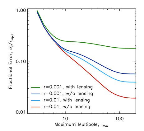
Figure 4.— Fractional error, $\sigma_{r}/r_{\rm input}$, on the determination of the value of $r$ as a function of maximum multipoles, $l_{\rm max}$. Here, $\sigma_{r}$ is the square-root of the second-order moment of the likelihood function given by Equation (5). (The foreground is not included. The full sky coverage is assumed.) From the top to bottom lines, we show $r_{\rm input}=0.001$ with and without the lensing noise, and $r_{\rm input}=0.01$ with and without the lensing noise, respectively. For the instrumental noise level, we have used 2 ${\mu}$K arcmin. Note that $\sigma_{r}/r_{\rm input}\sim 1$ at $l_{\rm max}=3$ does not mean that we do not detect $r$; on the contrary, we detect $r$ with high significance even at $l_{\rm max}=2$. Rather, it just means that the likelihood for $r$ is highly non-Gaussian and has a long tail toward large values of $r$ (see the top left panel of Figure 3). In other words, we detect $r$ with high statistical significance, but the value of $r$ is not determined very well.

Figure 4 shows the fractional error, $\sigma_{r}/r_{\rm input}$, on the determination of the value of $r$ as a function of $l_{\rm max}$. First, as one may expect from Figure 3, the fractional error for $r_{\rm input}=10^{-3}$ saturates at $l_{\rm max}\sim 10$ and does not improve further due to the lensing noise. For this case, while we can detect $r$ with high statistical significance, we can determine the actual value of $r$ to only $\sim 20$%. For $r_{\rm input}=10^{-2}$, we can determine the value of $r$ to $\sim 4$% at $l_{\rm max}=200$ (beyond which the fractional error no longer improves due to the lensing noise).

This study gives us an estimate of statistical errors on the measured values of $r$. On the other hand, the Galactic foreground gives us systematic errors (and bias). Now we shall turn to the foreground issue, which is the main subject of this paper.

3. Pixel-based foreground removal method

3.1. Motivation

The basic idea behind our methodology is simple: we have (at least) 3 polarized components on the sky that we know and have been detected by the WMAP: CMB, synchrotron emission, and thermal dust emission. As the synchrotron dominates at lower frequencies and the dust at higher frequencies, we use one map at a low frequency and another map at a high frequency as the foreground “templates.” We put the quotation marks here because these maps also contain the CMB. No external template maps are used in our method.

The WMAP team has applied this method for modeling the synchrotron: they used the lowest frequency (K-band, 23 GHz) map as a template, fitted it to the higher frequency maps (Ka, Q, V, and W bands), and subtracted from those maps. One can write this operation as

$$[Q^{\prime},U^{\prime}](\nu)=\frac{[Q,U](\nu)-\alpha_{S}(\nu)[Q,U](\nu=23~{}{\rm GHz})}{1-\alpha_{S}(\nu)},$$ (6)

where $Q^{\prime}$ and $U^{\prime}$ are the template-cleaned Stokes $Q$ and $U$ maps, respectively, and $\alpha_{S}$ is the best-fit synchrotron coefficient for a given frequency $\nu$. The denominator accounts for the fact that the K-band map also contains the CMB signal.

However, the WMAP team had to rely on an external map for modeling the dust emission, as the highest frequency, the W band (94 GHz), was not high enough for being a good template of the polarized dust emission. This issue would probably be resolved by the Planck satellite, which has higher frequency channels such as 217 and 353 GHz. Efstathiou et al. (2009) have studied this by using a simulated Planck 217 GHz or 353 GHz map as a template for dust, and a simulated 30 GHz map as a template for synchrotron. They find that this simple method removes the foreground efficiently, bringing the bias in $r$ down to a few times $10^{-3}$, which is much smaller than the expected statistical uncertainty on $r$ from Planck, $\sigma_{r}={\cal O}(10^{-2})$.

The goal of this paper is to put this method in the context of a next-generation, low noise (2 $\mu$K arcmin) polarization satellite experiment, and see if this method yields a promising result for measuring $r\sim 10^{-3}$ (which is easy to detect in the absence of foreground, as we just saw in Section 2).

3.2. “Template” cleaning method

Our methodology is similar to that given in Section 4.2 of Efstathiou et al. (2009).

The main parameter that we wish to extract from data is the tensor-to-scalar ratio, $r$. (We do not vary the tensor tilt, $n_{t}$.) The foreground coefficients, $\alpha$, are nuisance parameters that we wish to marginalize over. The foreground coefficients may be spatially varying.

Another nuisance parameter (for detecting $B$ modes) is the amplitude of the scalar $E$-mode power spectrum, which is by far the dominant source of CMB polarization. The signal power spectra are thus given as

$$C_{l}^{EE} = sc_{l}^{{\rm scalar},EE}+rc_{l}^{{\rm tensor},EE},$$ (7)

$$C_{l}^{BB} = rc_{l}^{{\rm tensor},BB},$$ (8)

where $c_{l}$ denotes the power spectra with $s=1$ and $r=1$. The fiducial value of $s$ is $s=1$.

We shall maximize the following likelihood function for estimating $r$, $s$, and $\alpha_{i}$:

$$\mathcal{L}(r,s,\alpha_{i})\propto\frac{\exp\left[-\frac{1}{2}{\bm{x}^{\prime}(\alpha_{i})}^{T}{\bm{C}^{-1}(r,s,\alpha_{i})}{\bm{x}^{\prime}(\alpha_{i})}\right]}{\sqrt{|{\bm{C}(r,s,\alpha_{i})}|}},$$ (9)

where

$$\bm{x}^{\prime}=\frac{[Q,U](\nu)-\sum_{i}\alpha_{i}(\nu)[Q,U](\nu^{\rm template}_{i})}{1-\sum_{i}\alpha_{i}(\nu)}$$ (10)

is a template-cleaned map. This is a generalization of Equation (6) for a multi-component case. In this paper, $i$ takes on “S” and “D” for synchrotron and dust, respectively, unless noted otherwise. For definiteness, we shall choose:

$$\nu=\mbox{100 GHz},$$

$$\nu^{\rm template}_{\rm S}=\mbox{60 GHz},$$

$$\nu^{\rm template}_{\rm D}=\mbox{240 GHz}.$$

These choices are somewhat arbitrary, but our preliminary optimization study indicates that this is a good configuration for achieving a smaller bias in $r$. A fuller optimization study, including more frequency channels, would require a more detailed specification of a given experiment (e.g., how many detectors one can fit in a given focal place; how low the detector noise can be as a function of frequencies), which is beyond the scope of this paper, but will be presented elsewhere.

The covariance matrix in pixel space, ${\bm{C}}$, for Stokes $Q$ and $U$ maps is given as

$${\bm{C}}(r,s,\alpha_{i})=r{\bm{c}}^{\rm tensor}+s{\bm{c}}^{\rm scalar}+\frac{{\bm{N}}_{1}+{\bm{N}}_{2}}{(1-\sum_{i}\alpha_{i})^{2}},$$ (11)

where ${\bm{c}}$ is the signal covariance matrix calculated from the theoretical power spectra, $c_{l}$, (see Appendix A) and the noise matrices, ${\bm{N}}_{1}$ and ${\bm{N}}_{2}$, are a noise covariance of a smoothed map (which is not diagonal) before the template cleaning is applied, and a small artificial diagonal noise matrix for a matrix regularization, respectively (see Section 4.1 for details).

For simplicity and clarity, we have ignored noise in template maps. For, if we assume that all three channels are similar in detector noise level, it is a good approximation, as $\alpha_{\rm D}\sim 0.08$ and $\alpha_{\rm S}\sim 0.25$, and the fractional contribution of the template noise to the covariance matrix is given by $\alpha^{2}_{i}$, i.e., 6% effect in the derived error bars. Note that this is equivalent to ignoring P in Section 4.2 of Efstathiou et al. (2009).

4. Simulation

4.1. CMB and detector noise

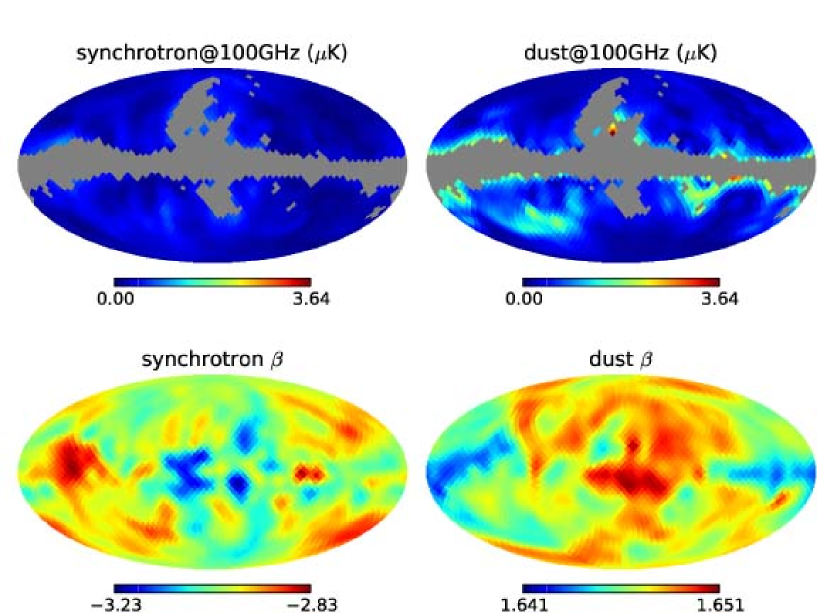
Figure 5.— Foreground maps from the Planck Sky Model (PSM; v1.6.2). The top left and top right panels show the polarization intensity maps ($P=\sqrt{Q^{2}+U^{2}}$ in units of $\mu$K) of synchrotron and dust, respectively. The dust polarization intensity has been multiplied by a factor of three to better approximate a more recent version of PSM. The lower left and lower right panels show the synchrotron index $\beta_{S}$ and the dust index $\beta_{D}$, respectively. Note a small range shown for $\beta_{D}$: the dust index does not vary much, but this is a built-in assumption of the PSM v1.6.2.

For CMB, we first generate the scalar and tensor polarization power spectra using the CAMB code (Lewis et al., 2000) with and without lensing contributions. We then generate Stokes $Q$ and $U$ maps at the Healpix resolution of $N_{\rm side}=128$. The signal map has been smoothed with a $30^{\prime}$ beam (FWHM), representing a low-angular-resolution CMB polarization satellite experiment targeting the primordial $B$ modes.

To this smoothed signal map, we add random Gaussian noise given by $\sigma_{0}/\sqrt{N_{\rm obs}(\hat{\bm{n}})}$ per pixel in the direction of $\hat{\bm{n}}$. Here, $\sigma_{0}$ is related to noise $w_{p}^{-1/2}$ as

$$\sigma_{0}=\frac{\pi}{10800}\frac{w_{p}^{-1/2}}{{\mu}{\rm K~{}arcmin}}\frac{1}{\sqrt{\Omega_{\rm pix}N_{\rm pix}^{-1}\sum_{i}N^{-1}_{\rm obs}(\hat{\bm{n}}_{i})}}~{}\mu{\rm K},$$ (12)

where $N_{\rm pix}=12(128)^{2}=196608$ is the total number of pixels at $N_{\rm side}=128$, and $N_{\rm obs}$ is the number of observations per pixel. We adopt $N_{\rm obs}$ from the “EPIC low-cost” (EPIC-LC) design (Bock et al., 2008). The noise is highest on the ecliptic plane and lowest on the ecliptic poles, similar to the $N_{\rm obs}$ pattern of the WMAP. Note that the absolute value of $N_{\rm obs}$ will cancel out in $\sigma_{0}/\sqrt{N_{\rm obs}(\hat{\bm{n}})}$ if we use the above formula: only the spatial distribution is taken from $N_{\rm obs}$, and the overall noise level is set by the assumed value of $w_{p}^{-1/2}$. We shall use $w_{p}^{-1/2}=2~{}\mu$K arcmin for the rest of this paper. For this low noise configuration, the results are not sensitive to the details of the $N_{\rm obs}$ pattern.

As we described at the end of Section 3, noise in template maps (at $\nu_{\rm S}=60$ GHz and $\nu_{\rm D}=240$ GHz) makes only a small contribution to the final covariance matrix. Therefore, for simplicity we add noise only to our CMB channel at 100 GHz.

We then apply an additional Gaussian smoothing to this signal-plus-noise map with 9.16 degrees (FWHM), which is $2.5$ times the pixel size at $N_{\rm side}=16$, and re-sample the smoothed map to $N_{\rm side}=16$. Finally, as the smoothed map at $N_{\rm side}=16$ is dominated by the scalar $E$-mode signal at all angular scales supported by the map resolution, the covariance matrix of this map is singular. In order to regularize the covariance matrix, we add an artificial, homogeneous white noise of $0.2~{}\mu{\rm K~{}arcmin}$ such that the map becomes noise dominated at the Nyquist frequency, $l_{\rm max}=3N_{\rm nside}-1=47$.

4.2. Foreground: Planck Sky Model

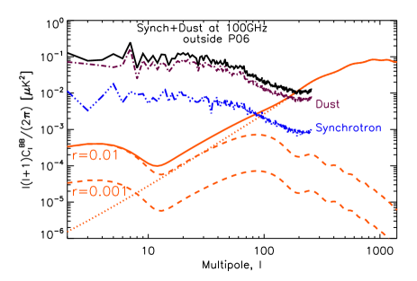
Figure 6.— $B$-mode polarization signal and foreground power spectra. The dashed lines show the primordial $B$-mode power spectra with the tensor-to-scalar ratio of $r=0.01$ and 0.001, while the dotted line shows the secondary $B$-mode power spectrum from gravitational lensing. We also show the $B$-mode power spectra of the dust (dot-dashed line) and synchrotron (triple-dot-dashed line) emission at 100 GHz outside the WMAP P06 mask ($N_{\rm side}=128$). (The measured foreground power spectra have been divided by $f_{\rm sky}=0.733$ to approximately correct for the mask, as well as by the pixel window function at $N_{\rm side}=128$.) The total (synch$+$dust) power spectrum is measured from the total map, which is slightly larger than the sum of the synchrotron and dust power spectra, as these two foreground components are spatially correlated. Note that the original PSM v1.6.2 dust map has the average polarization fraction of 1.5%, but we have multiplied the dust map by a factor of 3 to approximate a more recent dust template map adopted by the Planck collaboration.

For the Galactic foreground model, we use the Planck Sky Model (PSM; v1.6.2) developed by the Planck Component Separation Working Group (Working Group 2). Leach et al. (2008) describe the PSM for temperature, and Dunkley et al. (2009) for polarization.

The polarized synchrotron and dust emission are modeled as power-laws in antenna temperature:

$$[Q_{\rm synch},U_{\rm synch}](\nu,\hat{\bm{n}}) = g(\nu)[\tilde{Q}^{\rm PSM}_{\rm synch},\tilde{U}^{\rm PSM}_{\rm synch}](30~{}{\rm GHz},\hat{\bm{n}}),$$ (13)

$$\times\left(\frac{\nu}{30~{}{\rm GHz}}\right)^{\beta_{\rm S}(\hat{\bm{n}})},$$

$$[Q_{\rm dust},U_{\rm dust}](\nu,\hat{\bm{n}}) = g(\nu)[\tilde{Q}^{\rm PSM}_{\rm dust},\tilde{U}^{\rm PSM}_{\rm dust}](94~{}{\rm GHz},\hat{\bm{n}}),$$ (14)

$$\times\left(\frac{\nu}{94~{}{\rm GHz}}\right)^{\beta_{\rm D}(\hat{\bm{n}})}.$$

Here, $\tilde{Q}^{\rm PSM}$ and $\tilde{U}^{\rm PSM}$ are the PSM Stokes parameters in units of antenna temperature, and $g(\nu)\equiv(e^{x}-1)^{2}/(x^{2}e^{x})$ where $x=h\nu/k_{B}T_{\rm CMB}=\nu/56.780$ GHz converts the antenna temperature to thermodynamic temperature. (${Q}$ and ${U}$ are in units of thermodynamic temperature.)

For synchrotron, the position-dependent spectral index, $\beta_{\rm S}(\hat{\bm{n}})$, is calculated from the Haslam 408 MHz map (Haslam et al., 1981) and the three-year WMAP temperature map at 23 GHz (Page et al., 2007). The template maps at 30 GHz are taken from Miville-Deschênes et al. (2008).

For dust, the position-dependent spectral index, $\beta_{\rm D}(\hat{\bm{n}})$, as well as the unpolarized intensity map are taken from Model 8 of Finkbeiner et al. (1999). The polarization angles of dust approximately follow those of the synchrotron maps. The original PSM dust map has the average polarization fraction of 1.5% over the full sky, but we will multiply this map by a factor of 3 to approximate a more recent dust map used by the Planck collaboration.

Top panels of Figure 5 show the amplitude ($P=\sqrt{Q^{2}+U^{2}}$) of polarization intensity of synchrotron and dust at 100 GHz, while the bottom panels show the spectral indices, $\beta_{\rm S}$ and $\beta_{\rm D}$. After adding the above foreground maps (smoothed with a 9.16-degree beam at $N_{\rm side}=128$ and degraded to $N_{\rm side=16}$) to the CMB-plus-noise map, we mask the simulated sky by the WMAP P06 mask ($f_{sky}=73\%$)(Page et al., 2007).

The norm of the pixel vector, [$Q$,$U$], is $2259\times 2$, where 2259 is the number of pixels outside the P06 mask. In order to mask the covariance matrix, we use the technique described in Appendix D of Page et al. (2007): we compute an inverse of $6144\times 6144$ matrix and reduce it to $4518\times 4518$ matrix using Equation (D7) of Page et al. (2007). (Note that there is a typo in this equation: $D$ should be replaced by $D^{-1}$.)

In Figure 6, we show the $B$-mode power spectra measured from the PSM ($N_{\rm side}=128$) at 100 GHz outside the P06 mask. The total foreground power spectrum has $l(l+1)C_{l}^{BB}/(2\pi)\approx 10^{-1}~{}\mu{\rm K}^{2}$ at $l\lesssim 10$, which is 250 and 2500 times larger than the primordial $B$-mode spectra with $r=0.01$ and 0.001, respectively. The problem seems formidable; however, as we show below, the simple cleaning method can reduce the foreground-induced bias in $r$ to $\Delta r\approx 0.002(<0.001)$ with the P06(extended) mask.

5. Results

5.1. Fixing the scalar $E$-mode amplitude

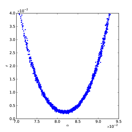
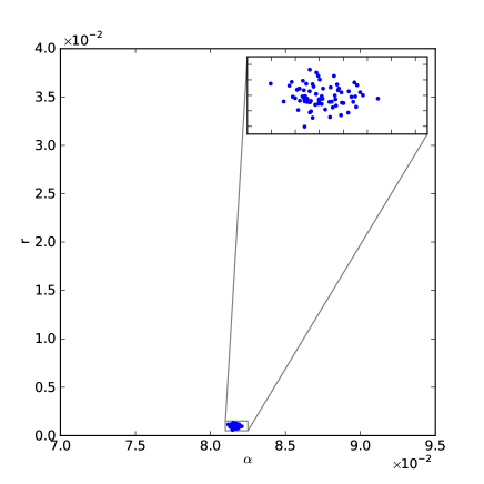
Figure 7.— Correlation between the tensor-to-scalar ratio, $r$, and the amplitude of dust, $\alpha_{\rm D}$. Left: The amplitude of the scalar $E$ modes is held fixed at $s=1$. Right: The amplitude of the scalar $E$ modes is treated as a nuisance parameter and marginalized over. The input tensor-to-scalar ratio is $r_{\rm input}=0.003$ and, for this figure only, the original PSM dust map (with an average polarization of $\sim 1.5\%$) is used.

Before we use our full likelihood function given by Equation (9), let us first try a simpler version and show that it actually fails.

For the moment (only within this subsection), we fix the amplitude of the scalar $E$ modes, i.e., $s=1$, and consider cleaning dust using a map at 240 GHz. (Synchrotron will not be discussed in this subsection.) Our model is thus

$$\left[Q,U\right](100) = \mbox{CMB}+\mbox{Dust(100)}+\mbox{Noise},$$ (15)

$$\left[Q,U\right](240) = \mbox{CMB}+\mbox{Dust(240)}.$$ (16)

As we described at the end of Section 3, we ignore noise at 240 GHz. We then fit the 240 GHz map to the 100 GHz map:

$$[Q^{\prime},U^{\prime}](100)=[Q,U](100)-\alpha_{\rm D}[Q,U](240).$$ (17)

Minimizing $\chi^{2}=[Q^{\prime},U^{\prime}]^{T}{\bm{C}}^{-1}[Q^{\prime},U^{\prime}]$ with respect to $\alpha_{\rm D}$ gives the following least-square solution:

$$\alpha_{\rm D}=\frac{[Q,U]^{T}(100){\bm{C}}^{-1}[Q,U](240)}{[Q,U]^{T}(240){\bm{C}}^{-1}[Q,U](240)}.$$ (18)

As the polarization signal is dominated by scalar $E$ modes, we can set $r=0$ when computing the covariance matrix ${\bm{C}}$ in this equation. (In practice, we used $r_{\rm input}$.) Finally, we maximize the likelihood given in Equation (9) with respect to $r$, with $s=1$ and $\alpha_{\rm D}$ given by the above least-square solution.

The left panel of Figure 7 shows the values of $r$ and $\alpha_{\rm D}$ obtained from many random realizations of noise and CMB skies. (The input tensor-to-scalar ratio is $r_{\rm input}=0.003$.) There is a clear correlation between $r$ and $\alpha_{\rm D}$, indicating a failure of this algorithm. This correlation is caused by a chance correlation between foreground and the dominant scalar $E$ modes (Chiang et al., 2008; Efstathiou et al., 2009). The correlation disappears when we set $C_{l}^{EE}=0$. This result motivates our treating the amplitude of scalar modes as a nuisance parameter.

The right panel of Figure 7 shows the results when $s$ is treated as a nuisance parameter and marginalized over. For this, we have maximized the likelihood given by Equation (9) by varying $r$, $s$, and $\alpha_{\rm D}$ simultaneously. The correlation between $r$ and $\alpha_{\rm D}$ has disappeared.

How well was dust cleaned? We have repeated this one-component foreground cleaning test for various values of $r_{\rm input}$ from 0.001 to 0.1. The results are shown in Table 1: in all cases, the method recovers $r$ successfully.

Table 1Dust-only Test

$r_{\rm input}$	mean($r$)	std($r$)
0.001	0.0011	0.0003
0.003	0.0030	0.0005
0.010	0.0102	0.0010
0.030	0.0296	0.0021
0.100	0.0991	0.0057

5.2. Cleaning synchrotron in multi-region

We are now ready to include synchrotron. Our model is

$$\left[Q,U\right](60) = \mbox{CMB}+\mbox{Synch(60)}+\mbox{Dust(60)}$$ (19)

$$\left[Q,U\right](100) = \mbox{CMB}+\mbox{Synch(100)}+\mbox{Dust(100)}$$ (20)

$$+\mbox{Noise}$$

$$\left[Q,U\right](240) = \mbox{CMB}+\mbox{Synch(240)}+\mbox{Dust(240)}$$ (21)

It turns out cleaning synchrotron is more challenging than cleaning dust, as the spatial distribution of synchrotron tends to be more extended above the Galactic plane than that of dust (see the top panels of Figure 5). We start by adding a mock synchrotron model (MSM) map to the PSM dust map. The MSM map has the same synchrotron polarization intensity across the sky as PSM at 30 GHz, but has a spatially invariant spectral index of $\beta=-3.0$ (where $\beta=-3.0$ is the average of spatially varying spectral index of PSM). With MSM plus PSM dust, $r$ is recoverd successfully; $\mbox{mean}(r)=0.0012$ and $0.0031$ for $r_{input}=0.001$ and $0.003$. (see the second and third columns of Table 2)

Even more problematic is the spatial variation of the synchrotron spectral index (see the bottom left panel of Figure 5), which causes a mismatch between a template map at 60 GHz and the actual synchrotron distribution at 100 GHz. When we use a single synchrotron coefficient, $\alpha_{\rm S}$, for the whole sky for the PSM model even without dust ($=$ synchrotron only), we find a bias in $r$ of order $\Delta r\approx 0.002$: $\mbox{mean}(r)=0.0028$ and $0.0120$ for $r_{\rm input}=0.001$ and 0.01, respectively (see the fourth and fifth columns of Table 2).

Table 2MSM and Synchrotron-only Tests (global and 48 regions)

$r_{\rm input}$	MSM		Global		48 Regions
	mean($r$)	std($r$)	mean($r$)	std($r$)	mean($r$)	std($r$)
0.001	0.0012	0.0004	0.0028	0.0005	0.0024	0.0005
0.003	0.0031	0.0006	0.0049	0.0008	0.0046	0.0007
0.010	-	-	0.0120	0.0011	0.0115	0.0011

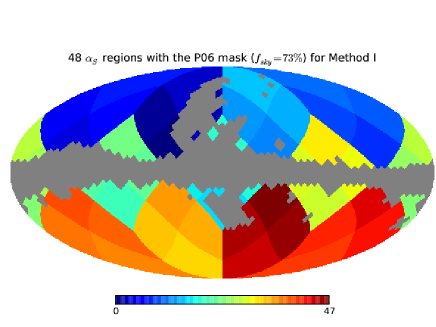
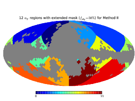
Figure 8.— (a) left: Method I. The P06 masked sky has been divided into 48 regions based on the Healpix map with $N_{\rm side}=2$. $f_{sky}$ of the mask is $73\%$. (b) right: Method II. The extended-masked sky has been divided into 12 regions based on the Healpix map with $N_{\rm side}=1$. $f_{sky}$ of the mask is $50\%$.

One way to mitigate this issue would be to extend the Galactic mask (Efstathiou et al., 2009). In addition, one may give up using a single synchrotron amplitude for the whole sky, and use multiple amplitudes depending on the locations on the sky. In this paper, we

1. continue to use the P06 mask, but divide the sky using the Healpix map with $N_{\rm side}=2$, as shown in Figure 8a and

2. extend the mask to $f_{sky}=50\%$ and divide the sky using the Healpix map with $N_{\rm side}=1$, as shown in Figure 8b.

We give the details of our definition of the extended mask in Appendix B. In short, we choose the threshold polarization intensity values at 60 and 240 GHz above which the pixels are masked, such that we retain 50% of the sky.

While we would probably do a better job at cleaning synchrotron if we divide the sky according to our knowledge of the polarized synchrotron measured by WMAP, for this paper we prefer to explore a simpler algorithm and see how well we can recover $r$.

Each region $I$ will be cleaned as (c.f., Equation (10))

$${\bm{x}}^{\prime}_{I}=\frac{[Q_{I},U_{I}](100)-\alpha_{\rm D}[Q_{I},U_{I}](240)-\alpha_{\rm S}^{I}[Q_{I},U_{I}](60)}{1-\alpha_{\rm D}-\alpha_{\rm S}^{I}}.$$ (22)

Note that we still use a single amplitude for dust on the whole sky. Similarly, the covariance matrix is given by (c.f., Equation (11))

$${\bm{C}}_{IJ}(r,s,\alpha_{i}) = r{\bm{c}}_{IJ}^{\rm tensor}+s{\bm{c}}_{IJ}^{\rm scalar}$$ (23)

$$+\frac{{\bm{N}}_{1,IJ}+{\bm{N}}_{2,IJ}}{(1-\alpha_{\rm D}-\alpha_{\rm S}^{I})(1-\alpha_{\rm D}-\alpha_{\rm S}^{J})},$$

where ${\bm{C}}_{IJ}$, ${\bm{c}}_{IJ}$ and ${\bm{N}}_{IJ}$ denote a block of matrices for pixels within regions $I$ and $J$.

The free parameters in the maximization are $r$, $s$, $\alpha_{\rm D}$, and $\alpha_{\rm S}^{i}$ (i=1…12(48)). In principle we wish to maximize the full likelihood function with respect to these parameters; however, in practice, this process is too time consuming to do brute-force, as varying each of these 15(51) parameters requires re-inverting a $4518\times 4518$ matrix. Therefore, we make one approximation: we fix $\alpha_{\rm D}$ and $\alpha_{\rm S}$ in the covariance matrix (Equation (23)) at the best-fit values, $\alpha_{\rm D}^{0}$ and $\alpha_{\rm S}^{i,0}$. This is a good approximation as long as the noise term is sub-dominant compared to the dominant scalar $E$-mode signal, which is always the case for our low-noise configuration. With this approximation,

$$\mathcal{L}(r,s,\alpha_{i})\propto\frac{\exp\left[-\frac{1}{2}{\bm{x}(\alpha_{i})}^{T}{\bm{C}(r,s;\alpha^{0}_{i})}^{-1}{\bm{x}(\alpha_{i})}\right]}{\sqrt{|{\bm{C}(r,s;\alpha^{0}_{i})}|}},$$ (24)

can be maximized with respect to $r$, $s$ and $\alpha_{i}$ where $i$ runs from 1 (dust) to 13(49) (synchrotron for 2 to 13(49)). We use the MINUIT package (James, 1988) for the maximization.

In the fourth and fifth columns of Table 2, we show the recovered values of $r$ for the synchrotron-only cases, in order to see if dividing the sky into 48 regions helps to reduce the bias in $r$ that we have just seen. We find that the bias has reduced, but not by much: $\Delta r=0.0018\to 0.0014$, $0.0019\to 0.0016$, and $0.0020\to 0.0015$ for $r_{\rm input}=0.001$, 0.003, and 0.01, respectively. This is probably due to the division not being tailored to match the distribution of synchrotron emission. While we keep this simple division and do not pursue a more complex division in this paper, we shall come back to this issue in the future work.

5.3. Recovering $r$

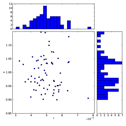
Figure 9.— Distribution of $r$ and $s$ obtained from 68 realizations $r_{\rm input}=0.003$ using Method I.

Table 3Recovered $r$ from Synchrotron and Dust cleaning

$r_{\rm input}$	mean($r$)	std($r$)	mean($r$)	std($r$)
0.001	0.0027	0.0005	0.0016	0.0006
0.003	0.0050	0.0008	0.0038	0.0009
0.010	0.0121	0.0013	0.0113	0.0015
0.030	0.0326	0.0021	-	-
0.100	0.1029	0.0053	-	-

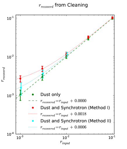
Figure 10.— Recovered values of $r$ (mean($r$)) and error bars (std($r$)) as a function of $r_{\rm input}$. The green points with error bars show the recovered $r$ from the dust-only results (Table 1); the red (cyan) points with error bars show the synchrotron-plus-dust results using Method I(II) (Table 3) A systematic bias of $\Delta r\approx 0.002(0.0006)$ is seen for the synchrotron-plus-dust results using Method I(II), which can be described by $r_{\rm recovered}=r_{\rm input}+(0.0018\pm 0.0004)((0.0006\pm 0.0004))$ (red(cyan) dotted line). We do not detect an offset for the dust-only results: $(0.0000\pm 0.0003)$ (green dashed line)

Now, we recover $r$ from the full dust-plus-synchrotron cases. In Figure 9, we show the distribution of $r$ and $s$ for all of 68 realizations that we have run with $r_{\rm input}=0.003$ using Method I. In Table 3, we show the recovered values of $r$ in the second and fourth columns. Comparing them to the input values, $r_{\rm input}$, in the first column, we conclude that our Method I recovers $r$ with a foreground-induced bias of $\Delta r\approx 0.002$, which is consistent with the bias we have just seen from the synchrotron-only cases. With Method II we recover $r$ with a much smaller bias of $\Delta r\approx 0.0006$. We visualize our results in Figure 10.

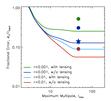
Figure 11.— The same as Figure 4, but the foreground-free predictions are made for simulated maps at $N_{\rm side}=16$ (as described in Section 2) and divided by $\sqrt{f_{\rm sky}}$ where $f_{\rm sky}=0.735$ for the P06 mask at $N_{\rm side}=16$. The filled circles use the error bars, $\sigma_{r}$, derived from our simulations with synchrotron and dust foreground cleaning (denoted as “std($r$)” in Table 3). The denominators, $r_{\rm input}$, are not the values recovered from the simulations, but the input values fixed at either 0.01 or 0.001. Each filled circle (foreground-cleaned result from simulations) should be compared to the corresponding line with the same color (foreground-free, analytical prediction). The star shows the foreground-free and lensing-free result from the simulation with $r_{\rm input}=0.001$, which agrees with the analytical prediction to within 10%.

The bias in $r$ is important, but the uncertainty in the recovered $r$ is equally important. In Figure 4, we have shown the predicted fractional errors on the determination of $r$, $\sigma_{r}/r_{\rm input}$, for idealistic full-sky, foreground-free cases. How would they look when synchrotron and dust are included and cleaned with our method? In Figure 11, we show the same figure but with the predictions made for the simulated CMB-plus-noise maps at $N_{\rm side}=16$ as described in Section 2, and scaled to the P06 mask. We also show $\sigma_{r}/r_{\rm input}$ where $\sigma_{r}$ is extracted from the simulations. First, when both the foreground and lensing noise are ignored, the simulation and the analytical prediction are in a good agreement (to within 10%) for $r_{\rm input}=0.001$ (see the star symbol in Figure 11). When the foreground is included, however, the error increases. For $r_{\rm input}=0.01$, the foreground cleaning increases the error by about 60%. We see larger discrepancies between the foreground-free predictions and the foreground-cleaned results for $r_{\rm input}=0.001$: the foreground-cleaned error is a factor of two larger than the foreground-free prediction; thus, the increase in the error due to foreground cleaning can be substantial when $r$ is as small as $10^{-3}$.

Further optimizations could be done, given the details of a given experiment, and we intend to explore this issue within the context of some specific experimental designs. Another improvement can be made by using $N_{\rm side}=32$ (or 64) map, so that the Nyquist frequency is close to (or beyond) the second bump of the $B$-mode spectrum and more information is used. Such analysis, however, would take $2^{6}=64$ ($4^{6}=4096$) times more computation.

6. Conclusions

In this paper, we have studied the pixel-based foreground cleaning method within the context of a next-generation, low-noise CMB polarization satellite. This method was originally applied to polarized data by the WMAP team (Page et al., 2007; Gold et al., 2009, 2010), and further investigated by Efstathiou et al. (2009) in the context of Planck.

Despite the simplicity of the method (namely, we have maps at 3 different frequencies, two of which are used for removing the synchrotron and dust emission), we are able to recover the input tensor-to-scalar ratio with only a small bias, $\Delta r\approx 0.002(<0.001)$ for the P06(extended) mask, which is dominated by the residual synchrotron emission. Further improvements should be straightforward: one can tune the Galactic mask, and divide the synchrotron fitting regions according to the actual distribution of the synchrotron spectral index in the Galaxy (rather than using the regular division shown in Figure 8). One may also increase the number of frequencies for measuring the spatial distribution of the synchrotron spectral index, provided that we have enough space on the focal plane. These will be investigated in the context of specific experimental designs such as LiteBIRD, and presented elsewhere.

Our study suggests that a detection of the primordial $B$-mode polarization at the level of $r\approx 10^{-3}$ should be possible with carefully optimized mask and $\alpha$ regions. Note that our statistical error and systematic bias becomes comparable with $f_{sky}=50\%$ mask case. However, let us mention one important caveat in our analysis. While our knowledge of the distribution and properties of the polarized synchrotron is fairly secure thanks to the WMAP data, our knowledge of the polarized dust emission, especially the spatial variation of the dust spectral index, is still highly limited. Therefore, the estimated bias in $r$ that we have presented in this paper cannot be too accurate. Fortunately, Planck will soon provide us with maps of the polarized dust emission with the unprecedented sensitivity; thus, we intend to revisit this issue once the Planck data become available.

Appendix A Signal Covariance matrix

Given power spectra, $c_{\ell}^{BB}$ and $c_{\ell}^{EE}$, components of the signal covariance matrix for $Q$ and $U$ can be computed analytically. We have

$${\bm{c}}(\hat{\bm{n}},{\hat{\bm{n}}^{\prime}})=\left(\begin{array}[]{cc}c_{QQ}(\hat{\bm{n}},{\hat{\bm{n}}^{\prime}})&c_{QU}(\hat{\bm{n}},{\hat{\bm{n}}^{\prime}})\\ c_{UQ}(\hat{\bm{n}},{\hat{\bm{n}}^{\prime}})&c_{UU}(\hat{\bm{n}},{\hat{\bm{n}}^{\prime}})\end{array}\right),$$

where

$$c_{QQ}(\hat{\bm{n}},{\hat{\bm{n}}^{\prime}}) = \sum_{l}c_{l}^{EE}w_{l}^{2}\sum_{m}W_{lm}(\hat{\bm{n}})W^{*}_{lm}({\hat{\bm{n}}^{\prime}})+\sum_{l}c_{l}^{BB}w_{l}^{2}\sum_{m}X_{lm}(\hat{\bm{n}})X^{*}_{lm}({\hat{\bm{n}}^{\prime}})$$

$$c_{QU}(\hat{\bm{n}},{\hat{\bm{n}}^{\prime}}) = \sum_{l}c_{l}^{EE}w_{l}^{2}\sum_{m}[-W_{lm}(\hat{\bm{n}})X^{*}_{lm}({\hat{\bm{n}}^{\prime}})]+\sum_{l}c_{l}^{BB}w_{l}^{2}\sum_{m}X_{lm}(\hat{\bm{n}})W^{*}_{lm}({\hat{\bm{n}}^{\prime}})$$

$$c_{UQ}(\hat{\bm{n}},{\hat{\bm{n}}^{\prime}}) = \sum_{l}c_{l}^{EE}w_{l}^{2}\sum_{m}[-X_{lm}(\hat{\bm{n}})W^{*}_{lm}({\hat{\bm{n}}^{\prime}})]+\sum_{l}c_{l}^{BB}w_{l}^{2}\sum_{m}W_{lm}(\hat{\bm{n}})X^{*}_{lm}({\hat{\bm{n}}^{\prime}})$$

$$c_{UU}(\hat{\bm{n}},{\hat{\bm{n}}^{\prime}}) = \sum_{l}c_{l}^{EE}w_{l}^{2}\sum_{m}X_{lm}(\hat{\bm{n}})X^{*}_{lm}({\hat{\bm{n}}^{\prime}})+\sum_{l}c_{l}^{BB}w_{l}^{2}\sum_{m}W_{lm}(\hat{\bm{n}})W^{*}_{lm}({\hat{\bm{n}}^{\prime}})$$

and

$$W_{lm}(\hat{\bm{n}}) \equiv (-1)[_{2}Y_{lm}(\hat{\bm{n}})+_{-2}Y_{lm}(\hat{\bm{n}})]/2,$$

$$X_{lm}(\hat{\bm{n}}) \equiv (-i)[_{2}Y_{lm}(\hat{\bm{n}})-_{-2}Y_{lm}(\hat{\bm{n}})]/2.$$

We have assumed that $E$ modes and $B$ modes are uncorrelated. Here, $w_{l}$ is a smoothing function which includes an experimental beam, a pixel window function, and any other smoothing applied to maps.

Appendix B Extended Mask

The resolution 4 ($r4$) mask is extended from the P06 mask by setting the threshold foreground polarization intensity values at 60 and 240 GHz above which the pixels are masked. The intensity of the pixel $i$ in the resolution 7 map is defined as

$$P_{i}(\nu)=\sqrt{Q_{i}^{2}(\nu)+U_{i}^{2}(\nu)}$$ (B1)

where $Q$ and $U$ are the sum of synchrotron and dust:

$$[Q_{i},U_{i}](\nu)=[Q_{i,{\rm synch}},U_{i,{\rm synch}}](\nu)+[Q_{i,{\rm dust}},U_{i,{\rm dust}}](\nu)$$ (B2)

using PSM (See Eqs. (13) and (14)).

An $r4$ pixel is masked if

1. median of $P_{i}(240)$ pixels in the $r4$ pixel exceeds Threshold I, or

2. maximum of $P_{i}(240)$ in the $r4$ pixel exceeds Threshold II, or

3. median of $P_{i}(60)$ pixels in the $r4$ pixel exceeds Threshold III, or

4. maximum of $P_{i}(60)$ in the $r4$ pixel exceeds Threshold IV.

Keeping $f_{sky}=50\%$, the values of the four thresholds are determined by minimizing the total foreground intensity in the residual map;

$$P_{\rm res}({\rm mask})=\sum_{i\notin{\rm mask}}\sqrt{Q^{2}_{{\rm res},i}+U^{2}_{{\rm res},i}}$$ (B3)

where

$$[Q_{{\rm res},i},U_{{\rm res},i}]=[Q_{i},U_{i}](100)-\alpha_{D}[Q_{i},U_{i}](240)-\alpha_{S}[Q_{i},U_{i}](60).$$ (B4)

$\alpha_{D}$ and $\alpha_{S}$ are given in the usual way by solving

$$\frac{\partial\chi^{2}}{\partial\alpha_{j}}=0,(j=D,S)$$ (B5)

where

$$\chi^{2}=[Q_{{\rm res},i},U_{{\rm res},i}]^{T}[Q_{{\rm res},i},U_{{\rm res},i}],(Q_{{\rm res},i}=U_{{\rm res},i}=0,i\in{\rm mask})$$ (B6)

The median and max. thresholds for the 240(60) GHz map determined this way are $19.2(1.42)$ and $38.4(2.11)\mu K.$ I.e., ${\rm Threshold~{}I}=19.2$, ${\rm II}=38.4$, ${\rm III}=1.42$, and ${\rm IV}=2.11~{}\mu$K. Note that we have defined an extended mask by using PSM maps without CMB or noise. In practice, both contributions would add noise spikes to the mask which need to be carefully examined. The noise contribution should be quite small given that we consider a low-noise ($2~{}\mu$K arcmin) experiment in this paper. The CMB contribution can be removed by taking the difference between different channels and defining the threshold values on the difference maps (in the same way that the WMAP team has created temperature masks). However, given $f_{sky}$, $P_{\rm res}({\rm mask})$ has a very broad bottom as a function of the thresholds. At the bottom, the shape of the mask is stable and our results are insensitive to the choice of the threshold values or the algorithm.

References

- Bock et al. (2008) Bock, J., Cooray, A., Hanany, S., Keating, B., Lee, A., Matsumura, T., Milligan, M., Ponthieu, N., Renbarger, T., & Tran, H. 2008, ArXiv e-prints
- Brown et al. (2009) Brown, M. L., Ade, P., Bock, J., Bowden, M., Cahill, G., Castro, P. G., Church, S., Culverhouse, T., Friedman, R. B., Ganga, K., Gear, W. K., Gupta, S., Hinderks, J., Kovac, J., Lange, A. E., Leitch, E., Melhuish, S. J., Memari, Y., Murphy, J. A., Orlando, A., O’Sullivan, C., Piccirillo, L., Pryke, C., Rajguru, N., Rusholme, B., Schwarz, R., Taylor, A. N., Thompson, K. L., Turner, A. H., Wu, E. Y. S., Zemcov, M., & The QUa D collaboration. 2009, ApJ, 705, 978
- Chiang et al. (2010) Chiang, H. C., Ade, P. A. R., Barkats, D., Battle, J. O., Bierman, E. M., Bock, J. J., Dowell, C. D., Duband, L., Hivon, E. F., Holzapfel, W. L., Hristov, V. V., Jones, W. C., Keating, B. G., Kovac, J. M., Kuo, C. L., Lange, A. E., Leitch, E. M., Mason, P. V., Matsumura, T., Nguyen, H. T., Ponthieu, N., Pryke, C., Richter, S., Rocha, G., Sheehy, C., Takahashi, Y. D., Tolan, J. E., & Yoon, K. W. 2010, ApJ, 711, 1123
- Chiang et al. (2008) Chiang, L., Naselsky, P. D., & Coles, P. 2008, Modern Physics Letters A, 23, 1489
- Coulson et al. (1994) Coulson, D., Crittenden, R. G., & Turok, N. G. 1994, Phys. Rev. Lett., 73, 2390
- Dunkley et al. (2009) Dunkley, J., Komatsu, E., Nolta, M. R., Spergel, D. N., Larson, D., Hinshaw, G., Page, L., Bennett, C. L., Gold, B., Jarosik, N., Weiland, J. L., Halpern, M., Hill, R. S., Kogut, A., Limon, M., Meyer, S. S., Tucker, G. S., Wollack, E., & Wright, E. L. 2009, ApJS, 180, 306
- Efstathiou et al. (2009) Efstathiou, G., Gratton, S., & Paci, F. 2009, MNRAS, 397, 1355
- Finkbeiner et al. (1999) Finkbeiner, D. P., Davis, M., & Schlegel, D. J. 1999, ApJ, 524, 867
- Fraisse et al. (2008) Fraisse, A. A., Brown, J., Dobler, G., Dotson, J. L., Draine, B. T., Frisch, P. C., Haverkorn, M., Hirata, C. M., Jansson, R., Lazarian, A., Magalhães, A. M., Waelkens, A., & Wolleben, M. 2008, ArXiv e-prints, arXiv:0811.3920
- Gold et al. (2009) Gold, B., Bennett, C. L., Hill, R. S., Hinshaw, G., Odegard, N., Spergel, D. N., Weiland, J., Dunkley, J., Halpern, M., Jarosik, N., Kogut, A., Komatsu, E., Larson, D., Meyer, S. S., Nolta, M., Wollack, E., & Wright, E. L. 2009, ApJS, 180, 265
- Gold et al. (2010) Gold, B. et al. 2010, Astrophys. J. Suppl., submitted
- Gorski et al. (2005) Gorski, K. M., Hivon, E., Banday, A. J., Wandelt, B. D., Hansen, F. K., Reinecke, M., & Bartlemann, M. 2005, ApJ, 622, 759
- Hamimeche & Lewis (2008) Hamimeche, S. & Lewis, A. 2008, Phys. Rev. D, 77, 103013
- Haslam et al. (1981) Haslam, C. G. T., Klein, U., Salter, C. J., Stoffel, H., Wilson, W. E., Cleary, M. N., Cooke, D. J., & Thomasson, P. 1981, A&A, 100, 209
- James (1988) James, F. 1988, MINUIT, Reference Manual, Version 94.1 (CERN, Geneva, Switzerland)
- Kamionkowski et al. (1997) Kamionkowski, M., Kosowsky, A., & Stebbins, A. 1997, Phys. Rev. D, 55, 7368
- Komatsu et al. (2010) Komatsu, E. et al. 2010, Astrophys. J. Suppl., submitted, arXiv:1001.4538
- Larson et al. (2010) Larson, D. et al. 2010, Astrophys. J. Suppl., submitted
- Leach et al. (2008) Leach, S. M., Cardoso, J., Baccigalupi, C., Barreiro, R. B., Betoule, M., Bobin, J., Bonaldi, A., Delabrouille, J., de Zotti, G., Dickinson, C., Eriksen, H. K., González-Nuevo, J., Hansen, F. K., Herranz, D., Le Jeune, M., López-Caniego, M., Martínez-González, E., Massardi, M., Melin, J., Miville-Deschênes, M., Patanchon, G., Prunet, S., Ricciardi, S., Salerno, E., Sanz, J. L., Starck, J., Stivoli, F., Stolyarov, V., Stompor, R., & Vielva, P. 2008, A&A, 491, 597
- Lewis et al. (2000) Lewis, A., Challinor, A., & Lasenby, A. 2000, ApJ, 538, 473
- Liddle & Lyth (2009) Liddle, A. R. & Lyth, D. H. 2009, The Primordial Density Perturbation: Cosmology, Inflation and the Origin of Structure (Cambridge University Press)
- Miville-Deschênes et al. (2008) Miville-Deschênes, M., Ysard, N., Lavabre, A., Ponthieu, N., Macías-Pérez, J. F., Aumont, J., & Bernard, J. P. 2008, A&A, 490, 1093
- Page et al. (2007) Page, L., Hinshaw, G., Komatsu, E., Nolta, M. R., Spergel, D. N., Bennett, C. L., Barnes, C., Bean, R., Doré, O., Dunkley, J., Halpern, M., Hill, R. S., Jarosik, N., Kogut, A., Limon, M., Meyer, S. S., Odegard, N., Peiris, H. V., Tucker, G. S., Verde, L., Weiland, J. L., Wollack, E., & Wright, E. L. 2007, ApJS, 170, 335
- Planck Blue Book (2005) Plank; The Scientific Program ESA-SCI(2005)1
- QUIET (2010) QUIET Collaboration: Bischoff, C., Brizius, A., Buder, I., Chinone, Y., Cleary, K., Dumoulin, R. N., Kusaka, A., Monsalve, R., Næss, S. K., Newburgh, L. B., Reeves, R., Smith, K. M., Wehus, I. K., Zuntz, J. A., Zwart, J. T. L., Bronfman, L., Bustos, R., Church, S. E., Dickinson, C., Eriksen, H. K., Ferreira, P. G., Gaier, T., Gundersen, J. O., Hasegawa, M., Hazumi, M., Huffenberger, K. M., Jones, M. E., Kangaslahti, P., Kapner, D. J., Lawrence, C. R., Limon, M., May, J., McMahon, J. J., Miller, A. D., Nguyen, H., Nixon, G. W., Pearson, T. J., Piccirillo, L., Radford, S. J. E., Readhead, A. C. S., Richards, J. L., Samtleben, D., Seiffert, M., Shepherd, M. C., Staggs, S. T., Tajima, O., Thompson, K. L., Vanderlinde, K., Williamson, R., & Winstein, B. 2010, ArXiv e-prints, arXiv:1012.3191
- Seljak & Zaldarriaga (1996) Seljak, U. & Zaldarriaga, M. 1996, ApJ, 469, 437
- Seljak & Zaldarriaga (1997) Seljak, U. & Zaldarriaga, M. 1997, Phys. Rev. Lett., 78, 2054
- Weinberg (2008) Weinberg, S. 2008, Cosmology (Oxford, UK: Oxford University Press)
- Zaldarriaga et al. (2008) Zaldarriaga, M., Colombo, L., Komatsu, E., Lidz, A., Mortonson, M., Oh, S. P., Pierpaoli, E., Verde, L., & Zahn, O. 2008, ArXiv e-prints, arXiv:0811.3918
- Zaldarriaga & Seljak (1998) Zaldarriaga, M. & Seljak, U. 1998, Phys. Rev., D58, 023003