Crossing $w=-1$ by a single scalar field coupling with matter and the observational constraints

Abstract

Motivated by Yang-Mills dark energy model, we propose a new model by introducing a logarithmic correction. we find that this model can avoid the coincidence problem naturally and gives an equation of state $w$ smoothly crossing $-1$ if an interaction between dark energy and dark matter exists. It has a stable tracker solution as well. To confront with observations based on the combined data of SNIa, BAO, CMB and Hubble parameter, we obtain the best fit values of the parameters with $1\sigma,2\sigma,3\sigma$ errors for the noncoupled model: $\Omega_{m}=0.276\pm 0.008^{+0.016+0.024}_{-0.015-0.022}$, $h=0.699\pm 0.003\pm 0.006\pm 0.008$, and for the coupled model with a decaying rate $\gamma=0.2$: $\Omega_{m}=0.291\pm 0.004^{+0.008+0.012}_{-0.007-0.011}$, $h=0.701\pm 0.002\pm 0.005\pm 0.007$. In particular, it is found that the non-coupled model has a dynamic evolution almost undistinguishable to $\Lambda$CDM at the late-time Universe.

PACS number: 95.36.+x, 98.80.Cq, 98.80.Es

1 Introduction

The accelerating expansion has been supported by observations of supernova observations [1, 2], cosmic microwave background radiation (CMB), and the large scale structure through the baryon acoustic oscillation (BAO). However, the physical origin of acceleration is still a challenging mystery. Within the framework of general relativity, this can be interpreted by a cosmic dark energy with negative pressure. The simplest dark energy model is the cosmological constant ($\Lambda$CDM), where the vacuum energy is responsible for the accelerating expansion. Whereas, it suffers from two problems degenerately. The first is the fine-tuning problem: The observed vacuum energy density of order $\sim 10^{-47}$ GeV⁴ is about $10^{121}$ orders of magnitude smaller than the value expected by quantum field theory for a cut-off scale being the Plank scale, and is still about $10^{44}$ orders smaller even for a cut-off scale being the QCD scale [3]. The second is the coincidence problem: The conditions in the early Universe have to be set very carefully in order for the energy density of the vacuum and that of the matter to be comparable today. To solve these problems, abundances of dynamical dark energy models have been proposed, such as scalar field [4, 5, 6, 7, 8, 9], vector field [10, 11, 12, 13], and decaying vacuum energy [14, 15], Holographic dark energy model [16, 17, 18, 19] and so on (see [3] for details). In quintessence of scalar field, the Lagrangian density has a standard form $\mathcal{L}=\frac{1}{2}(\nabla\phi)^{2}-V(\phi)$, which contains a canonical kinetic term and a potential term. Some particular forms of the potentials of quintessence [4, 5, 6] or the coupled quintessence with dark matter [20, 21, 22], can not only lead to the late time acceleration of the Universe, but also avoid the coincidence problem.

As well known, the quintessence always has an equation of state (EoS) $w$ larger than $-1$. However, there have been some preliminary evidences that the current value of $w$ may be less than $-1$, as indicated from observations [23, 24, 25, 26, 27, 28, 29]. On the other hand, the phantom field with a negative kinetic energy [30] predicts a EoS being always smaller than $-1$. Furthermore, another scalar field model with a noncanonical kinetic term called K-essence was proposed [31, 32, 33]. The Lagrangian is generally taken to be $\mathcal{L}=f(\phi)g(X)$, where $X=\frac{1}{2}(\nabla\phi)^{2}$. In [33], $f(\phi)\propto\phi^{-\alpha}$ and $g(X)$ is a polynomial of $X$, leading to $w>-1$ for $\alpha>0$ as a quintessence and $w<-1$ for $\alpha<0$ as a phantom. For the considerations of the EoS of dark energy tracking that of the background, one expect that the EoS of dark energy may be lager than $-1$ in early times and smaller than $-1$ in late times, i.e., $w$ crosses $-1$. If this is supported by further observations, many dark energy models would undergo a problem. Note that, even in K-essence model, $w$ can not cross $-1$ for a fixed $\alpha$. Is it possible to have a transit from quintessence to phantom? The particular interacting phantom dark energy could give smooth transit from $w>-1$ to $w<-1$ [34]. The non-minimal interaction between dark matter and dark energy with a single scalar field could also make possible to do the crossing of the phantom divide [35]. Besides, based on employment of two scalar fields, a class of models have been proposed, thereby using extra degrees of freedom [36, 37, 38].

In this paper, we propose to study a new dark energy model described by a single scalar field, whose Lagrangian density contains a logarithmic factor. We call it effective scalar field (ESF) dark energy model. Since the kinetic energy term is noncanonical, it should belong to a subclass of K-essence models. This is inspired by our previous work on the quantum effective Yang-Mills condensate (YMC) dark energy model [11, 39, 40, 41, 42, 43] with $\mathcal{L}_{eff}\propto F\ln F$ for 1-loop case [10, 11, 39, 40], where $F$ is the squared gauge field strength [44, 45, 10]. The nonlinear kinetic terms appear generically in the effective action in string and supergravity theories [46]. The appearance of a logarithmic correction in the field is generic for effective quantum theories, e.g., the Coleman-Weinberg potential [47], the effective gravity [48, 49], as well as the effective Yang-Mills field [44]. Since the nature of dark energy is still unknown, in the following, we will investigate the phenomenological properties of ESF model. Based on the observation of nearby galaxies [50], an interaction between dark energy and dark matter is favored since it would give a more rapid structure formation than predicted by the $\Lambda$CDM model [51]. So, we will also generally consider that an interaction between dark energy and matter exists. As will be seen, with one scalar field, the model provides a smooth dynamical transit from quintessence to phantom, with its $w$ going from $>-1$ at high reshifts to $<-1$ at low redshifts, if the field decays into matter. All the physical quantities involved in the model are smooth during the whole dynamical evolution. Moreover, the coincidence problem is also avoided in this model, since it has a stable attractor solution. But, unfortunately, the fine-tuning problem is still exist since a model parameter has to be tuned to accord with the low density of the dark energy component obtained through observations. We will demonstrate these afore-mentioned points, and also carry out a joint $\chi^{2}$ analysis for the model, confronting it with recent observations from SN Ia [53, 54, 55], BAO peak measurement of large scale structure from the Sloan Digital Sky Survey (SDSS) [56] and the Two Degree Field Galaxy Redshift Survey (2dFGRS) [57], the shift parameter of CMB [58], and the history of the Hubble parameter [59, 60, 61]. Throughout this paper, we adopt a unit with $c=1$. Greek indices $\mu,\nu,...$ range over 0 to 3, and Latin indices $i,j,...$ range over 1 to 3.

2 The effective scalar field model

We consider a spatially flat Universe described by Friedmann-Robertson-Walker metric

$$ds^{2}=dt^{2}-a^{2}(t)\delta_{ij}dx^{i}dx^{j},$$ (1)

where the scalar factor $a(t)$ is determined by the Friedmann equation:

$$H^{2}=\frac{8\pi G}{3}(\rho_{\phi}+\rho_{m}+\rho_{r}),$$ (2)

where $\rho_{\phi}$, $\rho_{m}$ and $\rho_{r}$ represent energy density of dark energy, matter and radiation, respectively, and $H=\dot{a}/a$ is the Hubble parameter. The dark energy is described by a scalar field $\phi$ with a Lagrangian density

$${\cal L}_{\phi}=\left(\frac{1}{2}(\nabla\phi)^{2}-V(\phi)\right)\ln\left|\frac{\frac{1}{2}(\nabla\phi)^{2}-V(\phi)}{\alpha e}\right|,$$ (3)

where $(\nabla\phi)^{2}=g^{\mu\nu}\partial_{\nu}\phi\partial_{\nu}\phi$, $V(\phi)$ is a function of $\phi$, $\alpha$ is a scale of energy density to be fixed by observations, and $\ln e=1$. ${\cal L}_{\phi}$ in Eq.(3) is formally similar to the Lagrangian density of the 1-loop effective YMC dark energy model [11]. Assuming $\phi$ is homogeneous and isotropic, and only depends on time, i.e., $\phi=\phi(t)$. The action is given by

$$S=\int d^{4}x\sqrt{-g}{\cal L}_{\phi},$$ (4)

where $g\equiv{\rm det}(g_{\mu\nu})$. The variation of the action (4) with respect to $\phi$ gives

$$\ddot{\phi}+\left(3\frac{\dot{a}}{a}+\frac{\dot{\varepsilon}}{\varepsilon}\right)\dot{\phi}+\frac{dV}{d\phi}=0,$$ (5)

where a dot denotes $d/dt$, and $\varepsilon\equiv\ln\left|(\frac{1}{2}\dot{\phi}^{2}-V)/\alpha\right|$. Note that, Eq.(5) differs from that of the quintessence model by the extra term $(\dot{\varepsilon}/\varepsilon)\dot{\phi}$ . When a coupling exists between ESF and matter, their dynamical evolution equations are given by

$$\dot{\rho}_{\phi}+3H(\rho_{\phi}+p_{\phi})=-\Gamma\rho_{\phi},$$ (6)

$$\dot{\rho}_{m}+3H\rho_{m}=\Gamma\rho_{\phi},$$ (7)

where $\Gamma$ denotes the energy transformation rate from ESF to matter. For simplicity, we assume $\Gamma$ is a constant. The radiation is an independent component and evolves as $\rho_{r}(t)\propto a^{-4}$.

In the following we focus on the simple case of $V=0$. The energy density and pressure are easily gained by the variation of action (4) with respect to $g^{\mu\nu}$:

$$\rho_{\phi}=\alpha(\varepsilon+1)e^{\varepsilon},~{}~{}~{}~{}~{}p_{\phi}=\alpha(\varepsilon-1)e^{\varepsilon},$$ (8)

with $\varepsilon=\ln{(\frac{1}{2}\dot{\phi}^{2}}/\alpha)>-1$ required by $\rho_{\phi}>0$. It is easy to prove that, for the non-coupled case ($\Gamma=0$), Eq. (6) reduces to Eq. (5) with the help of Eq. (8). The EoS is given by

$$w=\frac{p_{\phi}}{\rho_{\phi}}=\frac{\varepsilon-1}{\varepsilon+1}.$$ (9)

In high energy limit with $\varepsilon\gg 1$, $w\rightarrow 1$, different from the high energy behavior $w\rightarrow{1}/{3}$ of the YMC model [11]. At the critical point $\varepsilon=0$, one has $w=-1$. Furthermore, $w<-1$ will be arrived when $-1<\varepsilon<0$. Introducing dimensionless $x\equiv\rho_{m}/\alpha$ and $r\equiv\rho_{r}/\alpha$, Eqs. (6) and (7) read as

$$\varepsilon^{\prime}+\frac{6\varepsilon}{\varepsilon+2}+\frac{\gamma(\varepsilon+1)}{\varrho(\varepsilon+2)}=0,$$ (10)

$$x^{\prime}+3x-\frac{\gamma}{\varrho}(1+\varepsilon)e^{\varepsilon}=0,$$ (11)

where ${}^{\prime}\equiv{d}/{dN}$ with $N\equiv\ln a(t)$, $\gamma\equiv\Gamma/\left(\frac{8\pi G\alpha}{3}\right)^{\frac{1}{2}}$ is the dimensionless decaying rate, and $\varrho\equiv[x+r+e^{\varepsilon}(\varepsilon+1)]^{1/2}$. Given initial values ($\varepsilon_{i}$, $x_{i}$), Eqs. (10) and (11) can be solved for each $\gamma$. $\gamma>0$ means that dark energy decays into matter, and vice versa. In this paper, we assume that $\gamma$ is positive, since $\gamma<0$ will lead to a negative matter density in the future, which is unacceptable from the point of view of physics.

Firstly, we would like to discuss the simple case of the non-coupled $(\gamma=0)$ ESF model. To ensure the standard cosmology not being spoiled by the presence of dark energy, one may take $\rho_{\phi i}/\rho_{ri}\leq 10^{-2}$ at $z_{i}\simeq 10^{8}$. The outcome is that, for any $\varepsilon_{i}$ in a wide range $-1<\varepsilon_{i}\leq 55$ corresponding to $\rho_{\phi i}$ ranging over almost infinity orders of magnitude, the current status ($\Omega_{\phi},\Omega_{m})\simeq(0.73,0.27$) is always attained. So the coincidence problem is solved at the price of choosing a fixed $\alpha$. As can be seen in Fig.1 (a), different initial values of $\varepsilon_{i}=-0.9,0,10,50$, lead to the same density of the ESF at present time. During earlier stages the decreasing $\rho_{\phi}(z)$ is subdominant to $\rho_{r}(z)$ and $\rho_{m}(z)$. Note that $\rho_{\phi}(z)$ always levels off at a certain time, earlier for a smaller $\varepsilon_{i}$. Then, it surpasses $\rho_{r}$ at $z\sim 10$ and surpasses $\rho_{m}$ at $z\sim 1$, respectively. Whereas, the matter density $\rho_{m}(t)$ evolves independently as $\rho_{m}(t)\propto a(t)^{-3}$, since it does not couple with the ESF. Fig.1 (b) shows that $w$ will decrease and increase with time and approach $-1$ at the late-time for $\varepsilon_{i}>0$ and $\varepsilon_{i}<0$, respectively. Moreover, for $\varepsilon_{i}=0$, the ESF acts as the $\Lambda$CDM model exactly. Note that, in the above three cases, all the corresponding $w$ will stay at $-1$ in the future and never cross $-1$. It can be understood as follows. For $\gamma=0$, Eq. (10) has a solution:

$$\varepsilon^{2}e^{\varepsilon}=Aa^{-6},$$ (12)

where $A$ is an integration constant determined by the initial conditions. Except the particular case that $\varepsilon=0$, $A$ is always positive, i.e., the RHS of Eq. (12) will always be larger than 0. This indicates that $\varepsilon$ will never cross 0 no matter the initial value of $\varepsilon$ is positive or negative. According to Eq. (9), we know that $w$ can not cross $-1$ resulting from $\varepsilon$ failing to cross $0$. In the special case of $\varepsilon_{i}=0$, $A$ is fixed to be zero. Thus, $\varepsilon=0$ will be kept all the time, i.e., $w=-1$ is constant. Since $\varepsilon^{2}e^{\varepsilon}$ decays with the expansion Universe as $\propto a^{-6}$, $\varepsilon\rightarrow 0$ at $z=0$. Therefore, $\rho_{\phi}(z=0)\simeq\alpha\simeq 0.73\rho_{c}$, where $\rho_{c}$ is the critical density of the Universe. We find that, for the whole range of $\varepsilon_{i}$, the resulting dynamical evolution in the recent past $(z<30)$ is almost identical to that in $\Lambda$CDM with deviations $(\rho_{\phi}-\rho_{\Lambda})/\rho_{\Lambda}<10^{-4}$. The total EoS is $w_{tot}=\sum\Omega_{j}w_{j}$, where $j$ stands for the ESF, matter and radiation, respectively. In the future ($N\rightarrow\infty$), one has $\Omega_{r}\rightarrow 0$, $\Omega_{m}\rightarrow 0$ and $\Omega_{\phi}\rightarrow 1$. Hence, $w_{tot}=w=-1$, as shown in Fig.1 (b). That is, the Universe will do an exact de Sitter expansion, and there is no big rip event which some dark energy models would encounter. Note that, the interacting phantom dark energy could also avoid the big rip event [34].

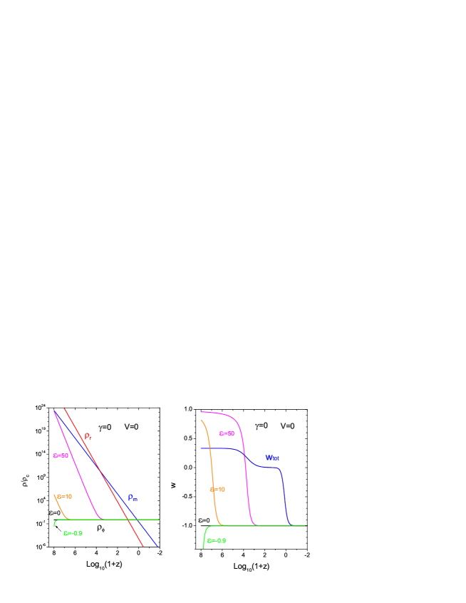
Figure 1: (a) $\rho_{\phi}(z)$, $\rho_{m}(z)$, and $\rho_{r}(z)$ in the non-coupled ESF model. For various initial values $\varepsilon_{i}$ the current status $\Omega_{\phi}=0.73$ and $\Omega_{m}=0.27$ is always achieved. (b) $w(z)$ does not cross $-1$ without the coupling.

Secondly, as an explicit example of ESF, we discuss the coupled case with $\gamma=0.2$. The initial conditions for the ESF and radiation are chosen the same as the case of non-coupled ESF. The initial condition for the matter is chosen a little differently from the non-coupled case in order to ensure the current status ($\Omega_{\phi},\Omega_{m})\simeq(0.73,0.27$). As illustrated in Fig.2 (a), the coincidence problem is also avoided in this case. The dynamic evolutions of the density of the coupled ESF are quite similar to those in the non-coupled ESF. However, $\rho_{m}$ levels off around $z\sim 0$ and will approach a constant instead of decaying as $\propto a(t)^{-3}$. This is caused by the coupling $\gamma\neq 0$. Fig. 2(b) plots evolutions of the corresponding $w(z)$. Due to the coupling, $w$ crosses $-1$, arrives at $w_{0}\simeq-1.05$ at present, and settles down to a constant value $w\simeq-1.07$ in future. The influence of the coupling $\gamma$ has been investigated, and computations show that a greater $\gamma$ yields a larger matter fraction $\Omega_{m}$ and a smaller EoS $w_{0}$ at present. We have also found an interesting relation: $\Omega_{\phi}=-1/w$ as $N\rightarrow\infty$, which is similar to YMC model [62]. This implies that the total EoS satisfies $w_{tot}=\Omega_{\phi}w=-1$ as $N\rightarrow\infty$. Thus, the coupled ESF model also predicts an exact de Sitter expansion in future, and the big rip event is avoided naturally. The parameter $\alpha$ in this case are determined by setting $\rho_{\phi}\simeq 0.73\rho_{c}$ at $z=0$, leading to $\alpha\simeq 0.76\rho_{c}$. Unfortunately, the particular choices of $\alpha$ being the same order of magnitude as $\rho_{c}$ let the ESF model still suffer from the fine-tuning problem.

We have carried out an analysis of dynamic stability of the set of Eqs. (10) and (11), and found that it has the fixed point $(\varepsilon_{c},x_{c})=(0,0)$ for $\gamma=0$ and $(\varepsilon_{c},x_{c})=(-0.0323,0.0625)$ for $\gamma=0.2$, respectively, as $N\rightarrow\infty$. Moreover, any perturbations $\delta\varepsilon$ and $\delta x$ are both decay as $e^{-3N}$ for $\gamma=0$, and decay as linear combinations of $e^{-3.3913N}$ and $e^{-2.8372N}$ for $\gamma=0.2$, respectively. Thus, the fixed points are stable, and then the attractor solutions of $\rho_{\phi}(t)$ are obtained for the above two cases. Aside the trajectory smoothness in phase space, the stability is problematic in single scalar field models [63]. Moreover, all the physical quantities in our models, such as $a(t)$, $\rho_{\phi}(t)$, and $w(t)$, are smooth from the initial moment up to the future.

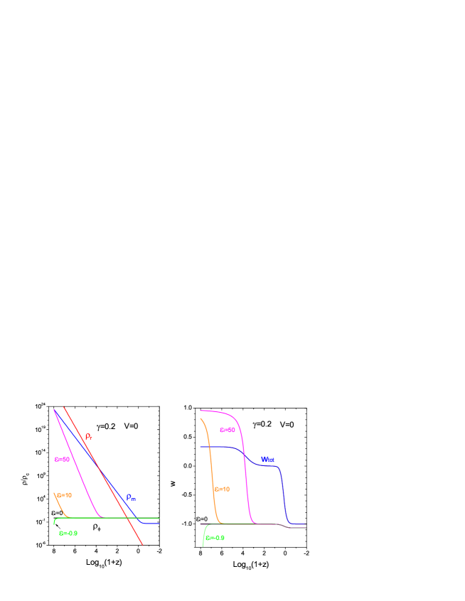
Figure 2: (a) $\rho_{\phi}(z)$, $\rho_{m}(z)$, and $\rho_{r}(z)$ in the coupled ESF model with $\gamma=0.2$. For various initial values $\varepsilon_{i}$ the current status $\Omega_{\phi}=0.73$ and $\Omega_{m}=0.27$ is always achieved. (b) $w(z)$ in the coupled model. Due to coupling, $w(z)$ is able to cross $-1$ at low redshifts.

3 Constraints from SN Ia, BAO, CMB and Hubble data

For a model of dark energy to be viable, it needs to confront or be constrained with observational data. Here we constrain the $V=0$ model with the latest observational data of the 557 SN Ia assembled in the Union2 compilation [55], the BAO measurement from SDSS [56] as well as 2dFGRS [57], the shift parameter of CMB from WMAP7 [58], and the the history of the Hubble parameter [59, 60, 61].

First, we compare the theoretical distance modulus to the observed ones compiled in [55]. The theoretical distance modulus is defined as

$$\mu_{th}(z)\equiv 5\log_{10}D_{L}(z)+\mu_{0},$$ (13)

where $D_{L}(z)=H_{0}(1+z)\int_{0}^{z}\frac{dz^{\prime}}{H(z^{\prime})}$ is the Hubble-free luminosity distance in a spatially flat Universe, and $\mu_{0}\equiv 42.38-5\log_{10}h$ with $h$ the Hubble constant in the unit of $100km/sec/Mpc$. The late-time Hubble rate of the effective scalar model is given by

$$H(z)=H_{0}[\Omega_{\phi}(z)+\Omega_{m}(z)]^{1/2},$$ (14)

where $\Omega_{i}(z)=\rho_{i}(z)/\rho_{c}$ for $i=\phi,m$. Since the evolution for $z\leq 10^{3}$ in this model is insensitive to the initial conditions, we choose $\varepsilon_{i}=10$ in the following calculations for concreteness. For the SN Ia data, the $\chi^{2}$ function is

$$\chi^{2}_{SN}(p_{s};\mu_{0})=\sum_{i=1}^{557}\frac{[\mu_{th}(z_{i})-\mu_{obs}(z_{i})]^{2}}{\sigma_{i}^{2}},$$ (15)

where $p_{s}$ stands for a set of parameters, such as $\Omega_{m}$. The nuisance parameter $\mu_{0}$ can be analytically marginalized over [64], so that one actually minimizes $\chi^{2}_{SN}(p_{s})$ instead of $\chi^{2}_{SN}(p_{s};\mu_{0})$.

Next, the BAO is revealed by a distinct peak in the large scale correlation function measured from the luminous red galaxies sample of the SDSS at $z=0.35$ [56], as well as in the 2dFGRS at $z=0.2$ [57]. The peaks can be associated to expanding spherical waves of baryonic perturbations. Each peak introduces a characteristic distance scale [56, 65]

$$D_{v}(z_{BAO})=\left[\frac{z_{BAO}}{H(z_{BAO})}\left(\int_{0}^{z_{BAO}}\frac{dz}{H(z)}\right)^{2}\right]^{1/3}.$$ (16)

The observational date from SDSS and 2dFGRS measurements yield $D_{v}(0.35)/D_{v}(0.2)=1.736\pm 0.065$ [57]. The best fit values for the model are given by minimizing [51, 52]

$$\chi_{BAO}^{2}(p_{s})=\frac{([D_{v}(0.35)/D_{v}(0.2)]_{th}-[D_{v}(0.35)/D_{v}(0.2)]_{obs})^{2}}{\sigma^{2}_{D_{v}(0.35)/D_{v}(0.2)}},$$ (17)

where $\sigma^{2}_{D_{v}(0.35)/D_{v}(0.2)}=0.065$.

As discussed in [66, 67], the first peak of the CMB spectrum of anisotropies, $l_{1}$, is more suitable to be used to test the interacting dark energy model than the CMB shift parameter, $R\equiv\sqrt{\Omega_{m}}D_{L}(z_{rec})/(1+z_{rec})$ [68, 69], where $z_{red}=1091$ [58] is redshift of recombination. Then, we use $l_{1}$, which is related to the angular scale, $l_{A}$, by [70]

$$l_{1}=l_{A}(1-\delta_{1}),$$ (18)

where

$$\delta_{1}=0.267\left(\frac{\bar{\rho}}{0.3}\right)^{0.1}$$ (19)

with $\bar{\rho}\equiv\rho_{r}(z_{rec})/\rho_{m}(z_{rec})$ the density ratio of radiation and matter at the time of recombination. The acoustic scale is defined as

$$l_{A}=\pi\int_{0}^{z_{rec}}\frac{dz}{H(z)}/\int_{z_{rec}}^{\infty}\frac{c_{s}dz}{H(z)},$$ (20)

where the sound velocity is $c_{s}=(3+\frac{9\Omega_{b}a}{4\Omega_{\gamma}})$, with $\Omega_{b}$ and $\Omega_{\gamma}$ the present density parameters of baryons and photons, respectively. With the observed position of the first peak $l_{1obs}=220.8\pm 0.7$ [71], the $\chi^{2}$ for CMB is

$$\chi_{CMB}^{2}(p_{s})=\frac{(l_{1th}-l_{1obs})^{2}}{\sigma_{l}^{2}},$$ (21)

where $\sigma_{l}=0.7$.

Finally, the Hubble parameter as a function of redshift $z$ can be written as

$$H(z)=-\frac{1}{1+z}\frac{dz}{dt}.$$ (22)

Then, once $dz/dt$ is known, $H(z)$ is obtained directly. Simon et al. [72] and Stern et al. [59] obtained $H(z)$ in the range of $0\leq z\leq 1.8$, using the differential ages of passively-evolving galaxies and archival data. Recently, some high precision measurements constrained $H(z)$ at $z=0$ from the observation of 240 Cepheid variables of rather similar periods and metallicities [60]. Besides, $H(z)$ at $z=0.24$, $0.34$ and $0.43$ is obtained [61] by using the BAO peak position as a standard ruler in the radial direction. We employ the twelve data in [60, 59] and the three data in [61]. The best fit values of the model parameters from observational Hubble data are determined by minimizing

$$\chi^{2}_{Hub}(p_{s})=\sum_{i=1}^{15}\frac{[H_{th}(z_{i})-H_{obs}(z_{i})]^{2}}{\sigma^{2}(z_{i})}$$ (23)

  

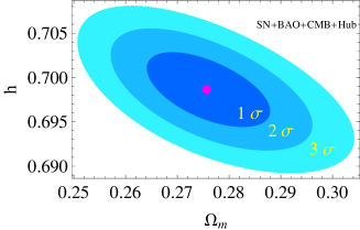
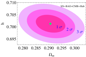
Figure 3: Left: The confidence contours for the pair of free parameters ($\Omega_{m},h$) obtained by constraining the non-coupled ESF model with the joint observational data from SN Ia, BAO, CMB and H(z). Right: The confidence contours of the same pair of parameters of the coupled ESF model with $\gamma=0.2$ obtained by the same observational data.

Thus, the total $\chi^{2}$ is combined as

$$\chi^{2}_{total}=\chi_{SN}^{2}+\chi_{BAO}^{2}+\chi_{CMB}^{2}+\chi_{Hub}^{2}.$$ (24)

As the likelihood function is determined as $\mathcal{L}\propto{\rm exp}(-\chi_{total}^{2}/2)$, the best fit values of $\Omega_{m}$ and $h$ follow from minimizing Eq.(24). Fig.3 shows the $68.3\%$ ($1\sigma$), $95.4\%$ ($2\sigma$) and $99.7\%$ ($3\sigma$) confidence contours in the $\Omega_{m}-h$ plane for both the ESF model with $\gamma=0$ and $\gamma=0.2$. For $\gamma=0$, the best fit values of 1-dimension up to $3\sigma$ confidence level are: $\Omega_{m}=0.276\pm 0.008^{+0.016+0.024}_{-0.015-0.022}$, $h=0.699\pm 0.003\pm 0.006\pm 0.008$, with a minimal $\chi^{2}_{totoal}=554.713$; while for $\gamma=0.2$, the results are: $\Omega_{m}=0.291\pm 0.004^{+0.008+0.012}_{-0.007-0.011}$, $h=0.701\pm 0.002\pm 0.005\pm 0.007$ with $\chi^{2}_{totoal}=556.033$. For comparison, we also calculate the case of $\Lambda$CDM and find it gives almost the same results as the non-coupled ESF model at a very high precision.

Now, we would like to compare these three dark energy models, i.e., $\Lambda$CDM, ESF models with $\gamma=0$ and $\gamma=0.2$. A conventional criterion for comparison is $\chi^{2}_{min}/dof$, in which the degree of freedom $dof=N-k$, whereas $N$ and $k$ are the number of data points and the number of free model parameters, respectively. We calculated the $\chi^{2}_{min}/dof$ for the three models, which can be seen in Table. I. Besides, there are other criterions for model comparison such as the Bayesian evidence [73, 74]. However, the Bayesian evidence is usually sophisticated. As an alternative, we can use some approximations of Bayesian evidence such as the so-called Bayesian Information Criterion (BIC) and Akaike Information Criterion (AIC), instead [75]. The BIC is defined as [76]

$${\rm{BIC}}=-2\ln{\mathcal{L}_{max}}+k\ln N,$$ (25)

and AIC is defined as [77]

$${\rm{AIC}}=-2\ln{\mathcal{L}_{max}}+2k,$$ (26)

where $\mathcal{L}_{max}$ is the maximum likelihood. In the Gaussian cases, $\chi^{2}_{min}=-2\ln{\mathcal{L}_{max}}$. So, the differences of BIC and AIC between two models are $\Delta{\rm{BIC}}=\Delta\chi^{2}_{min}+\Delta k\ln N$ and $\Delta{\rm{AIC}}=\Delta\chi^{2}_{min}+2\Delta k$, respectively. In Table. I, we also present the $\Delta{\rm{BIC}}$ and $\Delta{\rm{AIC}}$. One can find easily from Table. I that, the non-coupled ESF model and $\Lambda$CDM model not only have an almost identical evolution in the recent past ($z<30$), but also are undistinguishable in confronting with the combining observations from SN Ia, BAO, CMB and Hubble parameter. Moreover, for the coupled ESF model, it only gives a little larger $\chi^{2}_{\rm min}$ and little larger values of all the criterions for model comparison. Thus, $\gamma>0$ would be favored if further observations support $w<-1$ as indicated in Refs. [25], since the coupled and non-coupled ESF models perform similarly in $\chi^{2}$ analysis.

Table 1: Comparison of the three models considered in this work.

• Model	$\chi^{2}_{total}$	$\chi^{2}/dof$	$\Delta\rm{BIC}$	$\Delta\rm{AIC}$
  $\Lambda$CDM	554.713	0.970	0	0
  ESF ($\gamma=0$)	554.713	0.970	0	0
  ESF ($\gamma=0.2$)	556.033	0.972	1.32	1.32

4 Conclusions

Inspired by a generic feature of effective quantum fields, we have proposed a scalar field dark energy model, whose Lagrangian contains a logarithmic correction. It can be regarded as a special case of the generic K-essence models. For an initial value $\rho_{\phi i}$ ranging over almost infinite orders of magnitude, $\rho_{\phi}(t)$ tracks radiation and matter, and the current status ($\Omega_{\phi},\Omega_{m})\simeq(0.73,0.27$) is always attained. So the coincidence problem is solved if the parameter $\alpha$ is chosen in advance, but the fine-tuning problem remains. Moreover, $w$ smoothly crosses $-1$ if the ESF decays into matter. For a decay rate $\gamma=0.2$, the EoS arrives at $w_{0}\simeq-1.05$ at present. A greater $\gamma$ yields a larger $\Omega_{m}$ and a smaller $w_{0}$ at present. As $t\rightarrow\infty$, the expanding spacetime approaches the de Sitter as an asymptote, which is also a stable attractor, and there is no cosmic big rip. For the non-coupled model, $w$ approaches $-1$ but does not cross $-1$, and the dynamic behavior is almost the same as $\Lambda$CDM for low redshifts. In particular, for an initial $\varepsilon_{i}=0$, the model reduces to $\Lambda$CDM. Since the meaning of a non-zero $V(\phi)$ is unknown, we did not discuss the properties of the ESF model with $V(\phi)\neq 0$. Some particular forms of $V(\phi)$ would be investigated in the future study.

In confronting with observations of SN Ia, BAO, CMB and Hubble parameter, we plotted the confidence contours in the $\Omega_{m}-h$ plane for the ESF model with $\gamma=0$ and $\gamma=0.2$. The best fits of the parameters are: $\Omega_{m}=0.276\pm 0.008$ and $h=0.699\pm 0.003$ with $\chi^{2}_{totoal}=554.713$ for $\gamma=0$; $\Omega_{m}=0.291\pm 0.004$ and $h=0.701\pm 0.002$ with $\chi^{2}_{totoal}=556.033$ for $\gamma=0.2$. Furthermore, the non-coupled ESF model is distinguishable from $\Lambda$CDM model under present observations. Besides, we compared the three dark energy models studied in this work using $\chi^{2}/dof$, BIC and AIC . It is found that a non-coupled ESF model is a little more favored, however, the coupled model will survive if further observations support $w<-1$ strongly.

References

References

- [1] Riess A G et al 1998 Astron. J. 116 1009
- [2] Perlmutter S et al 1999 Astrophys. J. 517 565
- [3] Copeland E J, Sami M and Tsujikawa S 2006 Int. J. Mod. Phys. D 15 1753
- [4] Ratra B and Peebles P J E 1988 Phys. Rev. D 37 3406
- [5] Zlatev I , Wang L M and Steinhardt P J 1999 Phys. Rev. Lett. 82 896
- [6] Steinhardt P J , Wang L and Zlatev I 1999 Phys. Rev. D 59 123504
- [7] Ferreira P G and Joyce M 1998 Phys. Rev. D 58 023503
- [8] Dodelson S,Kaplinghat M and Steinhart E 2000 Phys. Rev. Lett. 85 5276
- [9] Carvalho F C, Alcaniz J S, Lima J A S and Silva R 2006 Phys. Rev. Lett. 97 081301
- [10] Zhang Y 1994 Phys. Lett. B 340 18
- [11] Zhang Y 2002 Gen. Relativ. Gravit. 34 2155
- [12] Kiselev V V 2004 Class. Quantum Grav. 21 3323
- [13] Armendariz-Picon C 2004 JCAP 07 007
- [14] Borges H A and Carneiro S 2005 Gen. Relativ. Gravit. 37 1385
- [15] Tong M L and Zhang Y 2009 Phys. Rev. D 80 023503
- [16] Cohen A G, Kaplan D B and Nelson A E 1999 Phys. Rev. Lett. 82 4971
- [17] Pavón D and Zimdahl W 2005 Phys. Lett. B 628 206
- [18] Li M 2004 Phys. Lett. B 603 1
- [19] Gao C, Wu F and Chen X 2009 Phys. Rev. D 79 043511
- [20] Amendola L 2000 Phys. Rev. D 62 043511
- [21] Chimento L P, Jakubi A S, Pavon D and Zimdahl W 2003 Phys. Rev. D 67 083513
- [22] Gonzalez T, Leon G and Quiros I 2006 Class Quantum. Grav. 23 3165
- [23] Corasaniti P S, Kunz M, Parkinson D, Copeland E J and Bassett B A 2004 Phys. Rev. D 70 083006
- [24] Alam U, Sahni V, Saini T D and Starobinsky A A 2004 Mon. Not. Roy. Astron. Soc. 354 275
- [25] Astier P et al 2006 Astron. Astrophys. 447 31
- [26] Conley A et al 2006 Astrophys. J. 644 1
- [27] Wood-Vasey W M et al 2007 Astrophys. J. 666 694
- [28] Davis T M et al 2007 Astrophys. J. 666 716
- [29] Freedman W L et al 2009 Astrophys. J. 704 1036
- [30] Caldwell R R 2002 Phys. Lett. B 545 23
- [31] Armendariz-Picon C, Mukhanov V and Steinhardt P J 2000 Phys. Rev. Lett. 85 4438
- [32] Armendariz-Picon C, Mukhanov V and Steinhardt P J 2001 Phys. Rev. D 63 103510
- [33] Chiba K, Okabe T, Yamaguchi M 2000 Phys. Rev. D 62 023511
- [34] Curbelo R, Gonzalez T and Quiros I 2006 Class. Quantum Grav. 23 1585
- [35] Gonzalez T and Quiros I 2008 Class. Quantum Grav. 25 175019
- [36] Feng B, Wang X L and Zhang X M 2005 Phys. Lett. B 607 35
- [37] Hu W 2005 Phys. Rev. D 71 047301
- [38] Zhao W and Zhang Y 2006 Phys. Rev. D 73 123509
- [39] Zhao W and Zhang Y 2006 Class. Quantum. Grav. 23 3405
- [40] Zhang Y, Xia T Y and Zhao W 2007 Class. Quantum. Grav. 24 3309
- [41] Xia T Y and Zhang Y 2007 Phys. Lett. B 656 19
- [42] Tong M L, Zhang Y and Xia T Y 2009 Int. J. Mod. Phys. D 18 797
- [43] Wang S, Zhang Y and Xia T Y 2008 JACP 10 037
- [44] Pagels H and Tomboulis E 1978 Nucl. Phys. B 143 485
- [45] Adler S and Piran T 1984 Rev. Mod. Phys. 56 1
- [46] Gross D and Witten E 1986 Nucl. Phys. B 277 1
- [47] Coleman S and Weinberg E 1973 Phys. Rev. D 7 1888
- [48] Parker L and Ravel A 1999 Phys. Rev. D 60 063512
- [49] Parker L and Ravel A 1999 Phys. Rev. D 60 123502
- [50] Peebles P J E and Nusser A 2010 Nature 465 565
- [51] Durán I, Pavón D and Zimdahl W 2010 JCAP 07 018
- [52] Xu L X and Lu J B 2010 JCAP 03 025
- [53] Kowalski M et al 2008 Astrophys. J. 686 749
- [54] Hicken M et al 2009 Astrophys. J. 700 1097
- [55] Amanullah R et al 2010 Astrophys. J. 716 712
- [56] Eisenstein D J et al 2005 Astrophys. J. 633 560
- [57] Percival W J et al 2010 Mon. Not. Roy. Astron. Soc. 401 2148
- [58] Komatsu E et al arXiv:1001.4538
- [59] Stern D, Jiménez R, Verde L, Kamionkowski M and Stanford S A 2010 JCAP 02 008
- [60] Riess A G et al 2009 Astrophys. J. 699 539
- [61] Gaztañaga E, Cabré A and Hui L 2009 Mon. Not. Roy. Astron. Soc. 399 1663
- [62] Zhao W 2009 Int. J. Mod. Phys. D 18 1331
- [63] Vikman A 2005 Phys. Rev. D 71 023515
- [64] Nesseris S and Perivolaropooulos L 2005 Phys. Rev. D 72 123519
- [65] Nesseris S and Perivolaropooulos L 2007 JCAP 01 018
- [66] Carneiro S, Dantas M A, Pigozzo C and Alcaniz J S 2008 Phys. Rev. D 77 083504
- [67] Pigozzo C, Dantas M A, Carneiro S and Alcaniz J S 2010 arXiv:1007.5290
- [68] Bond J R, Efstathoiu G and Tegmark M 1997 Mon. Not. Roy. Astron. Soc. 291 L33
- [69] Wang Y and Mukherjee P 2006 Astrophys. J. 650 1
- [70] Hu W et al 2001 Astrophys. J. 549 669
- [71] Hinshaw G et al 2007 Astrophys. J. Suppl. 170 228
- [72] Simon J, Verde L and Jiménez R 2005 Phys. Rev. D 71 123001
- [73] Liddle A R 2007 Mon. Not. Roy. Astron. Soc. Lett. 377 L74
- [74] Liddle A R 2009 Ann. Rev. Nucl. Part. Sci. 59 95
- [75] Wei H 2010 JCAP 08 020
- [76] Schwarz G 1978 Ann. Statist. 6 461
- [77] Akaike H 1974 IEEE Trans. Automatic Control 19 716