Computational approaches to Poisson traces associated to finite subgroups of $\Sp_{2n}(\CC)$

Abstract.

We reduce the computation of Poisson traces on quotients of symplectic vector spaces by finite subgroups of symplectic automorphisms to a finite one, by proving several results which bound the degrees of such traces as well as the dimension in each degree. This applies more generally to traces on all polynomial functions which are invariant under invariant Hamiltonian flow. We implement these approaches by computer together with direct computation for infinite families of groups, focusing on complex reflection and abelian subgroups of $\mathsf{GL}_{2}(\CC)<\Sp_{4}(\CC)$, Coxeter groups of rank $\leq 3$ and $A_{4},B_{4}=C_{4}$, and $D_{4}$, and subgroups of $\mathsf{SL}_{2}(\CC)$.

1. Introduction

Let $A$ be a Poisson algebra over $\mathbb{C}$. We are interested in linear functionals $A\rightarrow\mathbb{C}$ satisfying $\{a,b\}\mapsto 0$ for all $a,b\in A$. Such functionals are called Poisson traces on $A$. The space of Poisson traces is denoted by $\mathsf{HP}_{0}(A)^{*}$, and is dual to the vector space $\mathsf{HP}_{0}(A):=A/\{A,A\}$, known as the zeroth Poisson homology, which coincides with the zeroth Lie homology.

Here, we study the case where $A=\mathcal{O}_{V}^{G}$ is the algebra of $G$-invariant polynomial functions on a nonzero symplectic vector space $V$, for a finite subgroup $G<\Sp(V)$. We will let $2n>0$ denote the dimension of $V$. We also consider the larger space $\mathsf{HP}_{0}(\mathcal{O}_{V}^{G},\mathcal{O}_{V}):=\mathcal{O}_{V}/\{\mathcal{O}_{V}^{G},\mathcal{O}_{V}\}$, as well as its dual, $\mathsf{HP}_{0}(\mathcal{O}_{V}^{G},\mathcal{O}_{V})^{*}$, which is the space of functionals $\phi$ on $\mathcal{O}_{V}$ which are invariant under the flow of $G$-invariant Hamiltonian vector fields, i.e., $\phi(\{f,g\})=0$ for all $f\in\mathcal{O}_{V}^{G}$ and $g\in\mathcal{O}_{V}$. Note that $\mathsf{HP}_{0}(\mathcal{O}_{V}^{G},\mathcal{O}_{V})^{*}$ is a $G$-representation, and its $G$-invariants form the space of Poisson traces on $\mathcal{O}_{V}^{G}$.

In general, not very much is known about such Poisson traces. In [AFLS00], a related quantity was computed: the dimension of the space of Hochschild traces on $\mathcal{D}_{X}^{G}$ where $\mathcal{D}_{X}$ is the algebra of differential operators on $X\subseteq V$, a Lagrangian subspace. The algebra $\mathcal{D}_{X}^{G}$ is naturally a quantization of $\mathcal{O}_{V}^{G}$, and its Hochschild traces are defined as $\mathsf{HH}_{0}(\mathcal{D}_{X}^{G})^{*}:=(\mathcal{D}_{X}^{G}/[\mathcal{D}_{X}^{G},\mathcal{D}_{X}^{G}])^{*}$. More precisely, equip $\mathcal{O}_{V}$ with its natural grading by degree of polynomials and $\mathcal{D}_{X}$ with its natural filtration (which is known as the additive or Bernstein filtration). Then, $\operatorname{\mathsf{gr}}\mathcal{D}_{X}=\mathcal{O}_{V}$, and there is a canonical surjection $\mathsf{HP}_{0}(\mathcal{O}_{V}^{G})\twoheadrightarrow\operatorname{\mathsf{gr}}\mathsf{HH}_{0}(\mathcal{D}_{X}^{G})$, and similarly $\mathsf{HP}_{0}(\mathcal{O}_{V}^{G},\mathcal{O}_{V})\twoheadrightarrow\operatorname{\mathsf{gr}}\mathsf{HH}_{0}(\mathcal{D}_{X}^{G},\mathcal{D}_{X})$. As a result, the dimension of the space of Hochschild traces is a lower bound for the dimension of the space of Poisson traces. In some special cases, the lower bound is attained, i.e., the surjection is an isomorphism. For example, $\mathsf{HP}_{0}(\mathcal{O}_{V}^{G})\cong\operatorname{\mathsf{gr}}\mathsf{HH}_{0}(\mathcal{D}_{X}^{G})$ is known to hold when $V=\mathbb{C}^{2}$, and in [ES09b], the first and last authors generalized this to the case $V=\mathbb{C}^{2n}=(\mathbb{C}^{2})^{\oplus n}$ and $G=S_{n}\ltimes K^{n}$ for $K<\mathsf{SL}_{2}(\CC)$ (certain cases were shown previously in [But09], and this result was conjectured by Alev [But09, Remark 40]). In [ES], the same authors will show that $\mathsf{HP}_{0}(\mathcal{O}_{V}^{G})\cong\operatorname{\mathsf{gr}}\mathsf{HH}_{0}(\mathcal{D}_{X}^{G})$ when $G=S_{n+1}$ is a Weyl group of type $A_{n}$ acting on its reflection representation $V=\CC^{2n}$ (but not for the $D_{n}$ case).

The following explicit formula for $\mathsf{HH}_{0}(\mathcal{D}_{X}^{G},\mathcal{D}_{X})$ as a $G$-representation is an easy generalization of the main result of [AFLS00]. Let $\mathbb{C}[G]_{\operatorname{ad}}$ denote the $G$-representation with underlying vector space the group algebra $\mathbb{C}[G]$, but with the conjugation action of $G$.

Lemma 1.1.

As a $G$-representation, $\mathsf{HH}_{0}(\mathcal{D}_{X}^{G},\mathcal{D}_{X})$ is isomorphic to the subrepresentation of $\mathbb{C}[G]_{\operatorname{ad}}$ spanned by elements $g\in G$ such that $g-\operatorname{Id}$ is invertible.

We stress, however, that the above lemma does not say anything about the filtration on $\mathsf{HH}_{0}(\mathcal{D}_{X}^{G},\mathcal{D}_{X})$ and hence about the grading on $\operatorname{\mathsf{gr}}\mathsf{HH}_{0}(\mathcal{D}_{X}^{G},\mathcal{D}_{X})$. In the aforementioned cases in [ES09b] and [ES], $\mathsf{HP}_{0}(\mathcal{O}_{X}^{G})$ is computed along with its grading, so when it is also isomorphic to $\operatorname{\mathsf{gr}}\mathsf{HH}_{0}(\mathcal{D}_{X}^{G})$, one obtains the grading on the latter.

Although we will not use it, the argument of Lemma 1.1 applies more generally to show that $\mathsf{HH}_{*}(\mathcal{D}_{X}^{G},\mathcal{D}_{X})\cong\mathbb{C}[G]_{\operatorname{ad}}$ as $G$-representations, with $\mathsf{HH}_{j}(\mathcal{D}_{X}^{G},\mathcal{D}_{X})$ mapping to the span of elements $g$ such that $\operatorname{rk}(g-\operatorname{Id})=\dim V-j$. In particular, $\mathsf{HH}_{*}(\mathcal{D}_{X}^{G},\mathcal{D}_{X})$ is always finite-dimensional. This is not necessarily true for $\mathsf{HP}_{*}(\mathcal{O}_{V}^{G},\mathcal{O}_{V})$: see, e.g., [EG07, Theorem 2.4.1.(ii)], which implies that $\mathsf{HP}_{*}(\mathcal{O}_{V}^{G})$ is infinite-dimensional when $G$ is nontrivial and $V$ is two-dimensional.

However, thanks to [BEG04, §7] (see also [ES09a]), the space $\mathsf{HP}_{0}(\mathcal{O}_{V}^{G},\mathcal{O}_{V})$ is finite-dimensional. On the other hand, explicit upper bounds are known in only a few cases. The first aim of this paper is to prove explicit upper bounds, which allow us to compute precisely $\mathsf{HP}_{0}(\mathcal{O}_{V}^{G},\mathcal{O}_{V})$ and $\mathsf{HP}_{0}(\mathcal{O}_{V}^{G})$ for small enough $G$ and low enough dimension of $V$ with the help of computer programs.

More precisely, it is not very computationally useful to prove an upper bound on $\dim\mathsf{HP}_{0}(\mathcal{O}_{V}^{G},\mathcal{O}_{V})$, since this does not immediately render its computation finite. Instead, we find upper bounds on the top degree of $\mathsf{HP}_{0}(\mathcal{O}_{V}^{G},\mathcal{O}_{V})$ as a graded vector space. This renders the computation of $\mathsf{HP}_{0}(\mathcal{O}_{V}^{G},\mathcal{O}_{V})$ finite.

To prove such a bound, we use the following reformulation exploited in [BEG04, §7]. Given any Poisson algebra $A$ and any $f\in A$, the condition that a functional $\varphi\in A^{*}$ kills $\{f,A\}$ can be rewritten as $\xi_{f}(\varphi)=0$ where $\xi_{f}$ is the Hamiltonian vector field corresponding to $f$, which acts on $A$ by $\xi_{f}(g)=\{f,g\}$ and acts on $A^{*}$ by the negative dual. In the case that $A=\mathcal{O}_{V}$ is a polynomial algebra, we may canonically identify the graded dual $A^{*}$, defined by $(A^{*})_{i}:=(A_{-i})^{*}$, with $\mathcal{O}_{V^{*}}$. Call this isomorphism $F:A^{*}{\;\stackrel{{{}_{\sim}}}{{\to}}\;}\mathcal{O}_{V^{*}}$. Under this isomorphism,

(1.2) $$F(\xi_{f}(\varphi))=F_{D}(\xi_{f})F(\varphi),$$

where $F_{D}(\xi_{f})$ is a kind of Fourier transform of $\xi_{f}$: for every $v\in V^{*},w\in V$, and $m\geq 0$, $F_{D}(v^{m}\partial_{w})=w\partial_{v}^{m}$. Here, $\partial_{v},\partial_{w}$ are differentiation operators defined by $\partial_{w}(v)=v(w)=\partial_{v}(w)$. More generally, $F_{D}:\mathcal{D}_{V}{\;\stackrel{{{}_{\sim}}}{{\to}}\;}\mathcal{D}_{V^{*}}^{\mathrm{op}}$ is an anti-isomorphism of rings of differential operators, given by $v\mapsto\partial_{v}$ and $\partial_{w}\mapsto w$.

As a result, $\mathsf{HP}_{0}(\mathcal{O}_{V}^{G},\mathcal{O}_{V})^{*}$ is identified with the solutions $h\in\mathcal{O}_{V^{*}}$ of the differential equations

(1.3) $$F_{D}(\xi_{f})(h)=0,\forall f\in\mathcal{O}_{V}^{G}.$$

To help understand the main argument below, we will make the above explicit using coordinates (although we do not strictly need to do this—everything below can be formulated invariantly. We will at least take care to distinguish between vector spaces and their duals.) Suppose that $\mathcal{O}_{V}^{G}$ is generated as a commutative algebra by elements $h_{1},\ldots,h_{k}$, and $V=X\oplus Y$ is symplectic with complementary Lagrangians $X$ and $Y$. Let us write $V^{*}=X^{*}\oplus Y^{*}$, where the inclusions $X^{*},Y^{*}\subseteq V^{*}$ are defined by $X^{*}=Y^{\perp}$ and $Y^{*}=X^{\perp}$. Fix bases $(x_{1},\ldots,x_{n})$ and $(y_{1},\ldots,y_{n})$ of $X^{*}$ and $Y^{*}$, respectively, with dual bases $(x_{1}^{*},\ldots,x_{n}^{*})$ and $(y_{1}^{*},\ldots,y_{n}^{*})$ of $X$ and $Y$, and assume that $(x_{i}^{*},y_{j}^{*})=\delta_{ij}=-(y_{j}^{*},x_{i}^{*})$. In particular, $\mathcal{O}_{V}=\mathbb{C}[x_{1},\ldots,x_{n},y_{1},\ldots,y_{n}]$. This induces the isomorphism $V{\;\stackrel{{{}_{\sim}}}{{\to}}\;}V^{*}$ given by $x_{i}\mapsto y_{i}^{*}$ and $y_{i}\mapsto-x_{i}^{*}$, and hence the Poisson bracket $\{x_{i},y_{j}\}=\delta_{ij}=-\{y_{j},x_{i}\}$. Then, $\mathsf{HP}_{0}(\mathcal{O}_{V}^{G},\mathcal{O}_{V})^{*}\subseteq\mathcal{O}_{V^{*}}$ identifies with the solutions of the differential equations

(1.4) $$\sum_{i=1}^{n}\bigl{(}y_{i}^{*}F_{D}(\frac{\partial h_{j}}{\partial x_{i}})-x_{i}^{*}F_{D}(\frac{\partial h_{j}}{\partial y_{i}})\bigr{)}(g)=0.$$

Note that, in (1.4), we only needed the restriction of $F_{D}$ to $\mathcal{O}_{V}$,

(1.5) $$F_{D}:\mathbb{C}[x_{1},\ldots,x_{n},y_{1},\ldots,y_{n}]{\;\stackrel{{{}_{\sim}}}{{\to}}\;}\mathbb{C}[\partial_{x_{1}},\ldots,\partial_{x_{n}},\partial_{y_{1}},\ldots,\partial_{y_{n}}].$$

The reason why we wrote $\frac{\partial h_{j}}{\partial x_{i}}$ instead of $\partial_{x_{i}^{*}}(h_{j})$ above was to avoid confusion with the product of the two elements $\partial_{x_{i}^{*}},h_{j}\in\mathcal{D}_{V^{*}}$, which would not be in $\mathcal{O}_{V}$, and similarly with $\frac{\partial h_{j}}{\partial y_{i}}$.

Next, for every $v\in V^{*}$, we can evaluate the above equations at $v$:

(1.6) $$\sum_{i=1}^{n}\bigl{(}y_{i}^{*}(v)F_{D}(\frac{\partial h_{j}}{\partial x_{i}})-x_{i}^{*}(v)F_{D}(\frac{\partial h_{j}}{\partial y_{i}})\bigr{)}(g)(v)=0.$$

This shows that the Taylor coefficients $F(\partial_{x_{1}},\ldots,\partial_{x_{n}},\partial_{y_{1}},\ldots,\partial_{y_{n}})(g)(v)$ of $g$ at $v$ (for $F$ a polynomial) only depend on the class of $F$ in the quotient $R_{v}:=\mathbb{C}[\partial_{x_{1}},\ldots,\partial_{x_{n}},\partial_{y_{1}},\ldots,\partial_{y_{n}}]/J_{v}$ (and on $g$), where $J_{v}$ is the ideal generated by the constant-coefficient operators on the LHS of (1.6), i.e., the elements $D_{v^{\prime}}h_{1},\ldots,D_{v^{\prime}}h_{k}$ where $v^{\prime}\in V$ is the element corresponding to $v\in V^{*}$ via the symplectic form, and $D_{v^{\prime}}$ is the directional derivative operation $D_{v^{\prime}}:\mathcal{O}_{V}\to\mathcal{O}_{V}$. Note that $J_{v}$ does not actually depend on the choice of generators $h_{1},\ldots,h_{k}\in\mathcal{O}_{V}^{G}$, since if we adjoin another polynomial $h_{k+1}\in\mathcal{O}_{V}^{G}$ to the list $h_{1},\ldots,h_{k}$, the new equation (1.6) is already implied by the previous $k$ equations due to the Leibniz rule, $D_{v^{\prime}}(fg)=(D_{v^{\prime}}f)g+(D_{v^{\prime}}g)f$.

As a result, we deduce that

(1.7) $$\dim\mathsf{HP}_{0}(\mathcal{O}_{V}^{G},\mathcal{O}_{V})^{*}\leq\dim R_{v},\forall v\in V^{*}.$$

This is the upper bound found in [ES09a, Proposition 3.5] (with the Fourier transform of the proof found there), and gives a precise version of the proof that $\mathsf{HP}_{0}$ is finite-dimensional from [BEG04, §7], once one notices that $\dim R_{v}$ is finite for generic $v\in V^{*}$. However, the main drawback is that there is no relation, in general, between the grading on $\mathsf{HP}_{0}(\mathcal{O}_{V}^{G},\mathcal{O}_{V})$ and that on $R_{v}$. The first main goal of this paper is to overcome this problem.

Much of this paper will concern the special case where $G<\mathsf{GL}(X)<\Sp(V)$, where the embedding $\mathsf{GL}(X)<\Sp(V)$ is defined by sending $A\in\mathsf{GL}(X)$ to $A\oplus(A^{-1})^{*}\in\Sp(X\oplus Y)$.

We now outline the contents of the paper. First, §2 gives an elementary bound on $\dim R_{v}$ using regular sequences, using an argument we will need again in §3. We also apply these results in §2.1 to bound the number of irreducible finite-dimensional representations of filtered quantizations as well as the number of zero-dimensional symplectic leaves of filtered Poisson deformations, although this is not needed for the rest of the paper.

In §§3 and 4 we refine the argument outlined in the present section in two different ways to obtain computationally useful bounds on the top degree of $\mathsf{HP}_{0}(\mathcal{O}_{V}^{G},\mathcal{O}_{V})$. In §3, we apply the above argument in the case $v\in X^{*}$ and $G<\mathsf{GL}(X)<\Sp(V)$ to obtain an upper bound on the top degree of $\mathsf{HP}_{0}(\mathcal{O}_{V}^{G},\mathcal{O}_{V})$. In §4, for arbitrary $G$ (not necessarily preserving a Lagrangian subspace) and for arbitrary $v\in V$ such that $R_{v}$ is finite-dimensional, we define a square matrix $A_{v}$ of size $\dim R_{v}$ such that the dimension of the degree $m$ part $\dim\mathsf{HP}_{0}(\mathcal{O}_{V}^{G},\mathcal{O}_{V})^{*}_{m}$ is bounded by the dimension of the $m$-eigenspace of $A$. We do this by lifting generators $f_{1},\ldots,f_{N}$ of $R_{v}$ to differential operators $F_{1},\ldots,F_{N}$ on $V^{*}$, and considering the differential equations satisfied by the vector $(F_{1}(T),\ldots,F_{N}(T))$ for all $T\in\mathsf{HP}_{0}(\mathcal{O}_{V}^{G},\mathcal{O}_{V})^{*}$ upon evaluation on the line $\mathbb{C}\cdot v$.

Next, in §5, we will apply these results and computer programs [RS10b] written by two of the authors in Magma [BCP97] to obtain $\mathsf{HP}_{0}(\mathcal{O}_{V}^{G},\mathcal{O}_{V})$ for many groups $G$, including all finite subgroups of $\mathsf{SL}_{2}(\CC)$, the Coxeter groups of rank $\leq 3$ and types $A_{4},B_{4}=C_{4}$, and $D_{4}$, and the exceptional Shephard-Todd complex reflection groups $G_{4},\ldots,G_{22}<\mathsf{GL}_{2}<\Sp_{4}$ (except for $G_{18}$ and $G_{19}$, where we could only obtain $\mathsf{HP}_{0}(\mathcal{O}_{V}^{G})$ and without proof). Combining the latter with results of §7, we obtain a classification of complex reflection groups of rank two for which $\mathsf{HP}_{0}(\mathcal{O}_{V}^{G},\mathcal{O}_{V})\cong\operatorname{\mathsf{gr}}\mathsf{HH}_{0}(\mathcal{D}_{X}^{G},\mathcal{D}_{X})$ as well as those for which $\mathsf{HP}_{0}(\mathcal{O}_{V}^{G})\cong\operatorname{\mathsf{gr}}\mathsf{HH}_{0}(\mathcal{D}_{X}^{G})$, and give the Hilbert series in these cases.

In the final two sections, we explicitly compute $\mathsf{HP}_{0}(\mathcal{O}_{V}^{G},\mathcal{O}_{V})$, as well as its grading and $G$-structure, for several infinite families of groups in $\Sp_{4}$. Namely, in §6, we give an explicit description of $\mathsf{HP}_{0}(\mathcal{O}_{V}^{G},\mathcal{O}_{V})$ in the case that $G<\Sp_{4}$ is abelian (where it coincides with $\mathsf{HP}_{0}(\mathcal{O}_{V}^{G})$), classify such groups that have the property that $\mathsf{HP}_{0}(\mathcal{O}_{V}^{G})\cong\operatorname{\mathsf{gr}}\mathsf{HH}_{0}(\mathcal{D}_{X}^{G})$, and give the relevant Hilbert series. In §7, we explicitly compute $\mathsf{HP}_{0}(\mathcal{O}_{V}^{G},\mathcal{O}_{V})$ for the complex reflection groups $G=G(m,p,2)$, and classify those having the properties $\mathsf{HP}_{0}(\mathcal{O}_{V}^{G},\mathcal{O}_{V})\cong\operatorname{\mathsf{gr}}\mathsf{HH}_{0}(\mathcal{D}_{X}^{G},\mathcal{D}_{X})$ and $\mathsf{HP}_{0}(\mathcal{O}_{V}^{G})\cong\operatorname{\mathsf{gr}}\mathsf{HH}_{0}(\mathcal{D}_{X}^{G})$.

Throughout this article, $G$ always denotes a finite group, and $V$ a finite-dimensional symplectic vector space. The algebra $\mathcal{O}_{V}$ and the space $\mathsf{HP}_{0}(\mathcal{O}_{V}^{G},\mathcal{O}_{V})$ are nonnegatively graded, whereas their duals, $\mathcal{O}_{V^{*}}$ and $\mathsf{HP}_{0}(\mathcal{O}_{V}^{G},\mathcal{O}_{V})^{*}$, are nonpositively graded.

1.1. Acknowledgements

This work grew out of several projects supported by MIT’s Undergraduate Research Opportunities Program. The first author’s work was partially supported by the NSF grant DMS-1000113. The second author is a five-year fellow of the American Institute of Mathematics, and was partially supported by the ARRA-funded NSF grant DMS-0900233.

2. An elementary bound on dimension using Koszul complexes

We begin with an elementary explicit bound on the dimension of $\mathsf{HP}_{0}(\mathcal{O}_{V}^{G},\mathcal{O}_{V})$. While, for computational purposes, we ultimately want to bound its top degree, we include this both because it may be of independent interest, and because we will generalize it in §3.1 to give a bound also on the top degree. Additionally, in the next subsection we apply it to representation theory.

We will consider $J_{v}$ to be an ideal of $\mathcal{O}_{V}$ via (1.5). If $h_{1},\ldots,h_{2n}\in J_{v}$ is a collection of homogeneous elements which forms a regular sequence, i.e., $h_{i}$ is a nonzerodivisor in $\mathcal{O}_{V}/(h_{1},h_{2},\ldots,h_{i-1})$ for all $i$, then the Hilbert series of $R=\mathcal{O}_{V}/(h_{1},\ldots,h_{2n})$ can be computed using the associated Koszul complex, and one obtains

(2.1) $$h(R_{v};t)\leq h(R;t)=\frac{\prod_{i=1}^{2n}(1-t^{|h_{i}|})}{(1-t)^{2n}}.$$

Here we say that $\sum_{i}a_{i}t^{i}\leq\sum_{i}b_{i}t^{i}$ if $a_{i}\leq b_{i}$ for all $i$.

We can construct such a regular sequence from a regular sequence $g_{1},\ldots,g_{2n}\in\mathcal{O}_{V}^{G}$ using the following lemma, which essentially follows from [ES09a, Theorem 3.1]. We will actually state and prove it more generally.

Lemma 2.2.

Let $U$ be an arbitrary finite-dimensional vector space and $g_{1},\ldots,g_{\dim U}\in\mathcal{O}_{U}$ a regular sequence of homogeneous elements of degree $\geq 2$. Then, for generic $u\in U$, the directional derivatives $D_{u}g_{1},\ldots,D_{u}g_{\dim U}$ also form a regular sequence.

Remark 2.3.

In particular, the ideal in $\mathcal{O}_{U}$ generated by $D_{u}g_{1},\ldots,D_{u}g_{\dim U}$ has finite codimension for generic $u$. Specializing to the case that $U=V$ is symplectic of dimension $2n>0$, $G<\Sp(V)$ is finite, and $g_{1},\ldots,g_{2n}\in\mathcal{O}_{V}^{G}$, then for $v\in V^{*}$ and $u\in V$ the corresponding element by the symplectic form, this ideal is contained in $J_{v}$. Hence, this result strengthens the fact from [ES09a, §3] that $J_{v}$ has finite codimension for generic $v\in V^{*}$, once one notes that a regular sequence $g_{1},\ldots,g_{2n}\in\mathcal{O}_{V}^{G}$ of positively-graded homogeneous elements always exists (the elements must have degree $\geq 2$ unless $V^{G}\neq\{0\}$, in which case $J_{v}$ is generically the unit ideal).

Proof.

We will prove that, for generic $u$, the vanishing locus $Y_{u}$ of the functions $D_{u}g_{1},\ldots,D_{u}g_{\dim U}$ is $\{0\}$. Hence they form a complete intersection, and therefore a regular sequence (by standard characterizations of regular sequences; see, e.g., [Eis95, §§17, 18]). Note that $Y_{u}$ is nonempty and invariant under scaling, since $g_{1},\ldots,g_{\dim U}$ are homogeneous of degrees $\geq 2$. So we only need to prove that $\dim Y_{u}=0$.

The inclusion of polynomial algebras $\CC[g_{1},\ldots,g_{\dim U}]\subseteq\mathcal{O}_{U}$ defines a map $\phi:U\to\mathbb{A}^{\dim U}$. Since $g_{1},\ldots,g_{\dim U}$ define a regular sequence, $\phi$ is a finite map, i.e., $\mathcal{O}_{U}$ is a finite module over the polynomial subalgebra $\CC[g_{1},\ldots,g_{\dim U}]$. Now, consider the locus

$$Z:=\{(v,u)\in TU\mid v\in U,u\in T_{v}U,D_{u}g_{i}(v)=0,\forall i\}.$$

We are interested in the intersection $(U\times\{u\})\cap Z=(Y_{u}\times\{u\})$.

For every $0\leq r\leq\dim U$, consider the locus $U_{r}$ of $v\in U$ at which the map $\phi$ has rank $r$, i.e., the derivatives $D(g_{1})|_{v},\ldots,D(g_{\dim U})|_{v}$ evaluated at $v$ span a dimension $r$ subspace of $T_{v}^{*}U$. Then, the intersection $Z\cap(TU|_{U_{r}})$ is a vector bundle of rank $\dim U-r$ over $U_{r}$.

We claim that $\dim U_{r}\leq r$. This implies that $\dim Z\leq\dim U$. Thus, $(U\times\{u\})\cap Z=(Y_{u}\times\{u\})$ has dimension zero for generic $u$ (as $Y_{u}$ is always nonempty), as desired.

It remains to prove the claim that $\dim U_{r}\leq r$. Assume $U_{r}$ is nonempty. If we restrict $\phi$ to $U_{r}$, then we obtain a finite map $U_{r}\to\phi(U_{r})$. Generically, this restriction has rank $\dim U_{r}$, but by definition the rank is at most $r$. Hence, $\dim U_{r}\leq r$. ∎

We return to the case of the symplectic vector space $V$.

Corollary 2.4.

If $A\subseteq\mathcal{O}_{V}$ is a graded Poisson subalgebra containing a regular sequence $g_{1},\ldots,g_{2n}\in A$ of homogeneous, positively-graded elements, then

(2.5) $$\dim\mathsf{HP}_{0}(A,\mathcal{O}_{V})^{*}\leq\prod_{i=1}^{2n}(|g_{i}|-1).$$

Proof.

This follows immediately if none of the $g_{i}$ have degree one. On the other hand, if $g_{i}$ has degree one, then $\{g_{i},\mathcal{O}_{V}\}=\mathcal{O}_{V}$ since $\{g_{i},-\}$ is a directional derivative operator, so $\mathsf{HP}_{0}(A,\mathcal{O}_{V})=0$. ∎

For example, if $G<\mathsf{GL}(X)<\Sp(V)$ is a complex reflection group and $A=\mathcal{O}_{V}^{G}$, one could take $g_{1},\ldots,g_{n}$ and $g_{n-1},\ldots,g_{2n}$ to be homogeneous generators of the polynomial algebras $\mathcal{O}_{X}^{G}$ and $\mathcal{O}_{Y}^{G}$, where $V=X\oplus Y$ is as in the introduction. Then, we deduce that $\dim\mathsf{HP}_{0}(\mathcal{O}_{V}^{G},\mathcal{O}_{V})^{*}\leq\prod_{i=1}^{n}(|g_{i}|-1)^{2}<\prod_{i=1}^{n}|g_{i}|^{2}=|G|^{2}$. On the other hand, by Lemma 1.1, $\dim\mathsf{HH}_{0}(\mathcal{D}_{X}^{G},\mathcal{D}_{X})=|\{g\in G:g-\operatorname{Id}\text{ is invertible}\}|$, and as explained in the introduction, this gives a lower bound for $\dim\mathsf{HP}_{0}(\mathcal{O}_{V}^{G},\mathcal{O}_{V})$. Hence, we deduce

Corollary 2.6.

If $G<\mathsf{GL}(X)<\Sp(V)$ is a complex reflection group, then

(2.7) $$|\{g\in G:g-\operatorname{Id}\text{ is invertible}\}|\leq\dim\mathsf{HP}_{0}(\mathcal{O}_{V}^{G},\mathcal{O}_{V})^{*}<|G|^{2}.$$

However, in individual cases, one can do much better than this by directly computing $\dim R_{v}$.

2.1. Applications to representation theory and Poisson geometry

The material of this subsection is not needed for the rest of the paper; we include it since it is a natural consequence of the preceding results. Let $A=\bigoplus_{i\geq 0}A_{i}$ be a nonnegatively graded commutative algebra with a Poisson bracket of degree $-d<0$, i.e., $\{A_{i},A_{j}\}\subseteq A_{i+j-d}$. A filtered quantization is a filtered associative algebra $B=\bigcup_{i\geq 0}B_{\leq i}$ such that $\operatorname{\mathsf{gr}}B=A$ as a commutative algebra, $[B_{\leq i},B_{\leq j}]\subseteq B_{\leq(i+j-d)}$, and $\operatorname{\mathsf{gr}}_{i+j-d}[a,b]=\{\operatorname{\mathsf{gr}}_{i}a,\operatorname{\mathsf{gr}}_{j}b\}$ for all $a\in B_{\leq i},b\in B_{\leq j}$.

Next, given an arbitrary associative algebra $B$ and any finite-dimensional representation $\rho$ of $B$, the trace functional $\operatorname{Tr}(\rho):B\to\CC$ annihilates $[B,B]$ and hence defines an element of $\mathsf{HH}_{0}(B)^{*}$. Given nonisomorphic finite-dimensional irreducible representations $\rho_{1},\ldots,\rho_{m}$, the trace functionals $\operatorname{Tr}(\rho_{i})$ are linearly independent (by the density theorem), and hence $\dim\mathsf{HH}_{0}(B)\geq m$. In the situation that $B$ is a filtered quantization of $A$, one has a canonical surjection $\mathsf{HP}_{0}(A)\to\operatorname{\mathsf{gr}}\mathsf{HH}_{0}(B)$ (as in the case of $A=\mathcal{O}_{V}^{G}$ and $B=\mathcal{D}_{X}^{G}$ treated in the introduction). Hence, the number of irreducible representations of $B$ is at most $\dim\mathsf{HP}_{0}(A)$.

By the material from [ES09a] recalled in the introduction, we conclude:

Corollary 2.8.

[ES09a] If $G<\Sp(V)$ is finite, $B$ is an arbitrary filtered quantization of $\mathcal{O}_{V}^{G}$, and $v\in V^{*}$, then there are at most $\dim R_{v}$ irreducible finite-dimensional representations of $B$.

Applying Corollary 2.5, we immediately conclude:

Corollary 2.9.

If $g_{1},\ldots,g_{2n}\in\mathcal{O}_{V}^{G}$ is a regular sequence of homogeneous, positively-graded elements, then for every filtered quantization $B$ of $\mathcal{O}_{V}^{G}$, there are at most $\prod_{i}(|g_{i}|-1)$ irreducible finite-dimensional representations.

Applying Corollary 2.6, we conclude

Corollary 2.10.

If $G$ is a complex reflection group and $B$ a filtered quantization of $\mathcal{O}_{V}^{G}$, then there are fewer than $|G|^{2}$ irreducible finite-dimensional representations of $B$.

As pointed out after Corollary 2.6, in individual cases one can compute $\dim R_{v}$ directly, and it is typically much lower than this. Moreover, $\dim R_{v}$ is actually a bound on $\dim\mathsf{HP}_{0}(\mathcal{O}_{V}^{G},\mathcal{O}_{V})$, which is in general much larger than the upper bound $\dim\mathsf{HP}_{0}(\mathcal{O}_{V}^{G})$ above. Finally, again for $G$ a complex reflection group, when $B$ is a spherical symplectic reflection algebra quantizing $\mathcal{O}_{V}^{G}$ (see Remark 2.12 for the notion; note that these are also called spherical Cherednik algebras in the present case that $G$ is a complex reflection group), then it is actually known that there are fewer than $|\text{Irrep}(G)|$ irreducible finite-dimensional representations of $B$, where $\text{Irrep}(G)$ is the set of isomorphism classes of irreducible representations of $G$. This is much better than Corollary 2.10, in these cases. However, in general, there may exist more general quantizations $B$ than these.

The main goal of this paper is to introduce and apply techniques to explicitly compute $\mathsf{HP}_{0}(\mathcal{O}_{V}^{G})$ in many cases. This in particular provides the better upper bound $\dim\mathsf{HP}_{0}(\mathcal{O}_{V}^{G})$ on the number of irreducible finite-dimensional representations of quantizations $B$ of $\mathcal{O}_{V}^{G}$. These cases include many complex reflection groups, allowing us to replace the bound $|G|^{2}$ above by this improved bound. For example, by Theorem 5.24 below, applying also Lemma 1.1,

Corollary 2.11.

If $G<\mathsf{GL}_{2}<\Sp_{4}$ is one of the complex reflection groups $G(m,1,2),G(m,m,2)$, $G(4,2,2),G(6,2,2)$, or $G_{4},G_{5},G_{6},G_{8},G_{9},G_{14}$, or $G_{21}$, then $\mathsf{HP}_{0}(\mathcal{O}_{V}^{G})\cong\operatorname{\mathsf{gr}}\mathsf{HH}_{0}(\mathcal{D}_{X}^{G})$ has dimension equal to the number of conjugacy classes of elements $g\in G$ such that $g-\operatorname{Id}$ is invertible, i.e., $|\text{Irrep}(G)|-\text{Rank}(G)-1$, where $\text{Rank}(G)$ equals the number of conjugacy classes of complex reflections of $G$. Hence, this bounds the number of irreducible finite-dimensional representations of every filtered quantization of $\mathcal{O}_{\CC^{4}}^{G}$.

Note that, in the case $G(m,1,2)$, this is a special case of [ES09b, Corollary 1.2.1], which gives this upper bound in the case $G=G(m,1,n)$ for arbitrary $m$ and $n$ (as well as for $G=S_{n}\ltimes K^{n}$ for arbitrary $K<\mathsf{SL}_{2}(\CC)$). In the other cases, this bound is new. Similarly, the bounds $\dim\mathsf{HP}_{0}(\mathcal{O}_{V}^{G})$ for the other groups $G<\mathsf{GL}_{2}<\Sp_{4}$ considered in this paper are new.

Remark 2.12.

The filtered quantizations of $\mathcal{O}_{V}^{G}$ include all the associated noncommutative spherical symplectic reflection algebras (SRAs), defined in [EG02]. Recall that SRAs are certain deformations of $\mathcal{O}_{V}\rtimes G$ and spherical SRAs are of the form $B=e\widetilde{B}e$ where $e=\frac{1}{|G|}\sum_{g\in G}g\in\CC[G]$ is the symmetrizer element. Noncommutative spherical SRAs are those associated to those $\widetilde{B}$ obtainable by deforming $\mathcal{D}_{X}\rtimes G$ (these form a semi-universal family of deformations of $\mathcal{D}_{X}\rtimes G$).

Remark 2.13.

Similarly, one can make a statement about the commutative spherical SRAs. Namely, these are filtered commutative algebras $B$ equipped with a Poisson bracket satisfying $\{B_{\leq i},B_{\leq j}\}\subseteq B_{\leq i+j-d}$ such that $\operatorname{\mathsf{gr}}B=\mathcal{O}_{V}^{G}$ as a Poisson algebra. More generally, if $\operatorname{\mathsf{gr}}B=A$ where $B$ is a filtered commutative algebra equipped with a Poisson bracket satisfying $\{B_{\leq i},B_{\leq j}\}\subseteq B_{\leq i+j-d}$ and $A$ is equipped with the associated graded Poisson bracket of degree $-d<0$, then one obtains a canonical surjection $\mathsf{HP}_{0}(A)\twoheadrightarrow\operatorname{\mathsf{gr}}\mathsf{HP}_{0}(B)$. Hence, $\dim\mathsf{HP}_{0}(B)\leq\dim\mathsf{HP}_{0}(A)$. In particular, the number of zero-dimensional symplectic leaves (i.e., points whose maximal ideal is a Poisson ideal) of $B$ is dominated by $\dim\mathsf{HP}_{0}(A)$, the same bound as on the number of irreducible finite-dimensional representations of filtered quantizations of $A$, described in the above results. This is because the zero-dimensional symplectic leaves of $B$ all support linearly independent Poisson traces on $B$, given by evaluation at that point, and the space of Poisson traces on $B$ is the vector space $\mathsf{HP}_{0}(B)^{*}$. So, the number of zero-dimensional symplectic leaves of commutative spherical symplectic reflection algebras associated to $G$ is dominated by $\dim\mathsf{HP}_{0}(\mathcal{O}_{V}^{G})$, and hence by the same bounds described above.

3. The case $G<\mathsf{GL}_{n}<\Sp_{2n}$

As in the introduction, suppose $X$ is a Lagrangian in $V$ and $Y$ a complementary Lagrangian so that $V=X\oplus Y$. In this section we restrict to the case that $G<\mathsf{GL}(X)<\Sp(V)$. As in the introduction, we may equip $\mathcal{O}_{V}$ with a $G$-invariant bigrading, in which $|X^{*}|=(1,0)$ and $|Y^{*}|=(0,1)$. The total degree is the sum of these degrees. When an element $f$ has bidegree $(a,b)$, we will also say that $\deg_{X^{*}}f=a$ and $\deg_{Y^{*}}f=b$. Similarly, equip $\mathcal{O}_{V^{*}}$ with the bigrading in which $|X|=(-1,0)$ and $|Y|=(0,-1)$, and when $g\in\mathcal{O}_{V^{*}}$ has bidegree $(a,b)$, we say $\deg_{X}g=a$ and $\deg_{Y}g=b$. The total degree is again the sum of these degrees.

If we take $v\in X^{*}$, we can read off $\deg_{Y}g$ (for bihomogeneous $g\in\mathcal{O}_{V^{*}}$) from its Taylor expansion at $v$: it is given by the unique $j\geq 0$ such that there exists $F$ of degree $j$ in $Y^{*}$ such that $F(\partial_{x_{1}},\ldots,\partial_{x_{n}},\partial_{y_{1}},\ldots,\partial_{y_{n}})(g)(v)\neq 0$. Moreover, considering (1.6), we see that $J_{v}$ is a bihomogeneous ideal. Hence, we deduce that

$$\dim\{g\in\mathsf{HP}_{0}(\mathcal{O}_{V}^{G},\mathcal{O}_{V})^{*}\mid\deg_{Y}(g)=-j\}\leq\dim\{F\in R_{v}\mid\deg_{Y^{*}}F=j\},\quad\forall v\in X^{*},j\geq 0.$$

That is, we get a bound on the Hilbert series of $\mathsf{HP}_{0}(\mathcal{O}_{V}^{G},\mathcal{O}_{V})^{*}$ with respect to the $Y$-grading, in terms of the $Y^{*}$-grading on $R_{v}$ (for $v\in X^{*}$).

Next, we note that $\mathsf{HP}_{0}(\mathcal{O}_{V}^{G},\mathcal{O}_{V})$ is concentrated in bidegrees $(i,i),i\geq 0$, since it is annihilated by the action of the Hamiltonian vector field of $\sum_{i}x_{i}y_{i}$, i.e., the difference of degrees operator, $\xi_{\sum_{i}x_{i}y_{i}}(g)=(\deg_{Y}g-\deg_{X}g)g$ (for bihomogeneous $g\in\mathcal{O}_{V}$). Hence, the total degree of homogeneous elements of $\mathsf{HP}_{0}(\mathcal{O}_{V}^{G},\mathcal{O}_{V})^{*}$ is always twice the degree in $Y$ (equivalently, twice the degree in $X$). We deduce

Theorem 3.1.

For all $v\in X^{*}$,

(3.2) $$h(\mathsf{HP}_{0}(\mathcal{O}_{V}^{G},\mathcal{O}_{V});t)\leq h((R_{v},\deg_{Y});t^{2}).$$

Thus, the top degree of $(\mathsf{HP}_{0}(\mathcal{O}_{V}^{G},\mathcal{O}_{V})$ is dominated by twice the top degree of $R_{v}$ in $Y$.

Here, $(R_{v},\deg_{Y})$ denotes the ring $R_{v}$ equipped with its grading by degree in $Y$.

For the purpose of computing the top degree only, one can simplify the computation somewhat. Namely, the top degree of $R_{v}$ in $Y$ is the same as the top degree of $\overline{R_{v}}:=R_{v}/(X^{*})$. This follows since $R_{v}$ is bihomogeneous. So we obtain

(3.3) $$\text{topdeg}(\mathsf{HP}_{0}(\mathcal{O}_{V}^{G},\mathcal{O}_{V}))\leq 2\cdot\text{topdeg}(\overline{R_{v}}).$$

Explicitly, if $v^{\prime}\in Y$ is the element dual to $v\in X^{*}$ via the symplectic pairing, then $\overline{R_{v}}=\mathcal{O}_{Y}/(D_{v^{\prime}}g_{i})_{g_{i}\in\mathcal{O}_{Y}}$, where $\mathcal{O}_{Y}\subset\mathcal{O}_{V}$ are the functions of degree zero in $X^{*}$, which we also identify with $\mathcal{O}_{V}/(X^{*})$. That is, we can restrict to those $g_{i}$ which are only polynomials in the $y_{i}$. This has a particular advantage when $G$ is a complex reflection group, since there $\mathcal{O}_{Y}^{G}$ is a polynomial algebra whose structure is well known. We will exploit this below.

3.1. A bound on top degree using Koszul complexes

If we combine Theorem 3.1 with (2.1), we obtain

Corollary 3.4.

Suppose that $h_{1},\ldots,h_{2n}\in J_{v}$ are bihomogeneous and form a regular sequence, for $v\in X^{*}$. Then,

(3.5) $$h(\mathsf{HP}_{0}(\mathcal{O}_{V}^{G},\mathcal{O}_{V});t)\leq\frac{\prod_{i=1}^{2n}(1-t^{2\deg_{Y}(h_{i})})}{(1-t^{2})^{2n}}$$

The disadvantage of the above corollary is the need to verify the regular sequence property. Since the condition $v\in X^{*}$ is not generic, we cannot immediately apply Lemma 2.2. To ameliorate this, we can use an alternative approach, using the polynomial algebra in only the second half of the variables, $\mathcal{O}_{Y}$. Namely, rather than computing $R_{v}$, one can compute $\overline{R_{v}}=R_{v}/(X^{*})$ mentioned above, at the price of only bounding the top degree. Let us write $\overline{R_{v}}=\mathcal{O}_{Y}/\overline{J_{v}}$ where $\overline{J_{v}}=J_{v}/((X^{*})\cap J_{v})$.

Thus, if $h_{1},\ldots,h_{n}\in\overline{J_{v}}$ form a regular sequence in $\mathcal{O}_{Y^{*}}$, then

(3.6) $$\text{topdeg}(\mathsf{HP}_{0}(\mathcal{O}_{V}^{G},\mathcal{O}_{V}))\leq 2\,\sum_{i=1}^{n}(|h_{i}|-1).$$

Applying Lemma 2.2, we obtain:

Corollary 3.7.

If $g_{1},\ldots,g_{n}$ are homogeneous and form a regular sequence in $\mathcal{O}_{Y}^{G}$, then

(3.8) $$\text{topdeg}(\mathsf{HP}_{0}(\mathcal{O}_{V}^{G},\mathcal{O}_{V}))\leq 2\,\sum_{i}(|g_{i}|-2).$$

3.2. Complex reflection groups

In the case of complex reflection groups, $\mathcal{O}_{Y}^{G}$ is a polynomial algebra generated by homogeneous elements whose degrees are well known ([ST54]; see also [BMR98, Appendix 2]). Thus, in this case, we can apply Corollary 3.7 to generators $g_{1},\ldots,g_{n}$ of $\mathcal{O}_{Y}^{G}$. We thus deduce from Corollary 3.7 explicit bounds on the top degree of $\mathsf{HP}_{0}$:

Corollary 3.9.

The top degrees of $\mathsf{HP}_{0}(\mathcal{O}_{V}^{G},\mathcal{O}_{V})$ for complex reflection groups $G$ are at most:

$S_{n+1}$:	$n(n-1)$	$G(m,p,n)$, $m,n>1$:	$n(n-1)m+2mn/p-4n$	$G(m,1,1)$:	$2(m-2)$

$G_{4}$:	$12$	$G_{5}$:	$28$	$G_{6}$:	$24$	$G_{7}$:	$40$	$G_{8}$:	$32$	$G_{9}$:	$56$	$G_{10}$:	$64$
$G_{11}$:	$88$	$G_{12}:$	$20$	$G_{13}$:	$32$	$G_{14}$:	$52$	$G_{15}$:	$64$	$G_{16}$	$92$	$G_{17}$:	$152$
$G_{18}$:	$172$	$G_{19}$:	$232$	$G_{20}$:	$76$	$G_{21}$:	$136$	$G_{22}$:	$56$	$G_{23}$:	$24$	$G_{24}$:	$36$
$G_{25}$:	$42$	$G_{26}$:	$60$	$G_{27}$:	$84$	$G_{28}$:	$40$	$G_{29}$:	$72$	$G_{30}$:	$112$	$G_{31}$:	$112$

$G_{32}$:	$152$	$G_{33}$:	$80$	$G_{34}$:	$240$	$G_{35}$:	$60$	$G_{36}$:	$112$	$G_{37}$:	$224$

Remark 3.10.

Since the elements $g_{1},\ldots,g_{n}$ can be extended to a generating set for $\mathcal{O}_{V}$ by elements in the ideal $(X^{*})$, e.g., the corresponding generators of $\mathcal{O}_{X}^{G}$, the directional derivatives $D_{v^{\prime}}g_{1},\ldots,D_{v^{\prime}}g_{n}$ actually generate $\overline{J_{v}}\subseteq\mathcal{O}_{Y}$. Hence, the above bounds coincide with those obtained from $R_{v}$ itself using Theorem 3.1, and we lose nothing by applying the regular sequence arguments. This is in stark contrast to the estimate $\dim R_{v}<|G|^{2}$ of Corollary 2.6 (or even $\dim R_{v}\leq\prod_{i}(|g_{i}|-1)^{2}$), where one can do much better, in general, by computing $\dim R_{v}$ directly.

In the case $S_{n+1}$, the above bound was found by [Mat95], up to the equivalence of [RS10a, Theorem 1.5.1]; in the other cases, the bounds are new (except for the rank one case, $G(m,1,1)$, where $\mathsf{HP}_{0}(\mathcal{O}_{V}^{G},\mathcal{O}_{V})\cong\mathsf{HP}_{0}(\mathcal{O}_{V}^{G})$ is known to have dimension $2(m-2)$). Using the methods of this paper, we have computed the actual top degree in the cases of rank $\leq 2$ (with the possible exception of $G_{18},G_{19}$) as well as for certain Coxeter groups of higher rank, which generally differs substantially from the above. See Remark 7.45 for the top degree in the cases $G(m,p,2)$, and Theorem 5.25 for the top degree in some of the exceptional cases $G_{4},\ldots,G_{22}$.

4. The system of invariant Hamiltonian vector fields restricted to a line

Now, let $G<\Sp(V)$ and $v\in V^{*}$ be arbitrary. Although we know that elements in $\mathsf{HP}_{0}(\mathcal{O}_{V}^{G},\mathcal{O}_{V})^{*}$ are determined by their Taylor coefficients by representatives of $R_{v}$, in general the grading on $R_{v}$ is unrelated to the grading on $\mathsf{HP}_{0}(\mathcal{O}_{V}^{G},\mathcal{O}_{V})^{*}$ (note that $R_{v}$ is obtained by evaluating at $v$, which in particular replaces some polynomials on $V^{*}$ which have nonzero grading by numbers). To fix this problem, we will use $R_{v}$ to construct a local system on the line $\mathbb{C}\cdot v$ and make use of the Euler vector field, which multiplies by the (correct) degree on $\mathsf{HP}_{0}(\mathcal{O}_{V}^{G},\mathcal{O}_{V})^{*}$.

Let $f_{1},\ldots,f_{N}$ be a homogeneous basis for $R_{v}$, and let $F_{1},\ldots,F_{N}\in\mathcal{D}_{V^{*}}$ be differential operators on $V$ such that $(\operatorname{\mathsf{gr}}F_{i})|_{T^{*}_{v}V^{*}}\equiv f_{i}\pmod{J_{v}}$. Here, restricting $\operatorname{\mathsf{gr}}F_{i}\in\mathcal{O}_{T^{*}V^{*}}$ to $T^{*}_{v}V^{*}$ means evaluating the coefficients of the principal symbol $\operatorname{\mathsf{gr}}F_{i}$ of $F_{i}$ at the point $v$, obtaining an element of $\mathcal{O}_{T^{*}_{v}V^{*}}\cong\mathbb{C}[\partial_{x_{1}},\ldots,\partial_{x_{n}},\partial_{y_{1}},\ldots,\partial_{y_{n}}]$. For instance, we can let each $F_{i}$ be a constant-coefficient differential operator corresponding to a lift of $f_{i}$ to $\mathbb{C}[\partial_{x_{1}},\ldots,\partial_{x_{n}},\partial_{y_{1}},\ldots,\partial_{y_{n}}]$.

Claim 4.1.

For every $\phi\in\mathcal{D}_{V^{*}}$, there exists an operator of the form $\psi=\sum_{i}c_{i}F_{i}$ for $c_{i}\in\mathbb{C}$, such that $\phi(g)|_{\mathbb{C}\cdot v}=\psi(g)|_{\mathbb{C}\cdot v}$ for all $g\in\mathsf{HP}_{0}(\mathcal{O}_{V}^{G},\mathcal{O}_{V})^{*}$ (i.e., solutions of (1.4)).

In other words, the derivatives of solutions $g\in\mathcal{O}_{V^{*}}$ of (1.4), evaluated on the line $\mathbb{C}\cdot v$, depend only on the $F_{i}(g)$.

Using the claim, for every $\xi\in\mathcal{D}_{V^{*}}$, there exists an $N$ by $N$ matrix $C_{\xi}\in\mathrm{Mat}_{N}(\mathbb{C})$ such that

(4.2) $$(\xi\circ F_{1}(g),\ldots,\xi\circ F_{N}(g))|_{\mathbb{C}\cdot v}=C_{\xi}(F_{1}(g),\ldots,F_{N}(g))|_{\mathbb{C}\cdot v},\forall g\in\mathsf{HP}_{0}(\mathcal{O}_{V}^{G},\mathcal{O}_{V})^{*}.$$

In particular, if $\xi$ is the Euler vector field, i.e., $\xi(g)=\deg(g)\cdot g$, and if the $F_{i}$ are homogeneous (under the $\mathbb{C}^{*}$ action on $V$, i.e., $\deg u=-1$ for all $u\in V$, and $\deg\partial_{w}=1$ for all $w\in V^{*}$) of degrees $d_{1},\ldots,d_{N}\geq 0$, and $g\in\mathsf{HP}_{0}(\mathcal{O}_{V}^{G},\mathcal{O}_{V})^{*}$ is homogeneous, then

(4.3) $$C_{\xi}(F_{1}(g),\ldots,F_{N}(g))|_{\mathbb{C}\cdot v}-(d_{1}F_{1}(g),\ldots,d_{N}F_{N}(g))|_{\mathbb{C}\cdot v}=\deg(g)(F_{1}(g),\ldots,F_{N}(g))|_{\mathbb{C}\cdot v},$$

i.e., $\deg(g)$ is an eigenvalue of the matrix $B_{\xi}:=C_{\xi}-\mathrm{Diag}(d_{1},\ldots,d_{N})$, and $(F_{1}(g),\ldots,F_{N}(g))|_{\mathbb{C}\cdot v}$ is an eigenvector. Here $\mathrm{Diag}(d_{1},\ldots,d_{N})$ denotes the diagonal matrix with entries $d_{1},\ldots,d_{N}$. Now, for $\lambda\in\mathbb{C}$ and $C$ a square matrix, let $E_{\lambda}(C)$ denote the $\lambda$-eigenspace of $C$. We obtain

Theorem 4.4.

For arbitrary $v\in V^{*}$, degree $d_{i}$ lifts $F_{i}$ of generators $f_{i}$ of $R_{v}$ to $\mathcal{D}_{V^{*}}$, and $C_{\xi}$ satisfying (4.2) for $\xi$ the Euler vector field,

(4.5) $$h(\mathsf{HP}_{0}(\mathcal{O}_{V}^{G},\mathcal{O}_{V})^{*};t)\leq\sum_{i\leq 0}\dim E_{i}(B_{\xi})t^{i},\quad B_{\xi}:=C_{\xi}-\mathrm{Diag}(d_{1},\ldots,d_{N}).$$

It seems that the theorem has the disadvantage that many choices are involved: in particular, there are many possible choices of the matrix $C_{\xi}$. We claim nonetheless that, up to conjugation, the set of possible $B_{\xi}$ only depends on the choice of line $\mathbb{C}\cdot v$, and not on the choice of $f_{i}$ and $F_{i}$. Changing the $f_{i}$ and $F_{i}$ amounts to a combination of linear changes of basis (which change $C_{\xi}$ by the corresponding linear changes of basis), adding homogeneous elements to $F_{i}$ of the same degree as $F_{i}$ which send $\mathsf{HP}_{0}(\mathcal{O}_{V}^{G},\mathcal{O}_{V})^{*}$ to elements which are zero along $\mathbb{C}\cdot v$ (this does not change $C_{\xi}$), or multiplying the $F_{i}$ by homogeneous polynomials in $\mathcal{O}_{V^{*}}$ (which does not change $B_{\xi}$). Hence, the set of possible matrices $B_{\xi}$ is independent of these choices up to conjugation, and depends only only the line $\mathbb{C}\cdot v$. Thus, the same is true for the set of possible bounds (i.e., possible polynomials on the RHS of (4.5)).

Still, even for fixed $v$, there are in general several nonconjugate choices of $B_{\xi}$. This is because, in general, $N$ may exceed $\dim\mathsf{HP}_{0}(\mathcal{O}_{V}^{G},\mathcal{O}_{V})$, and so the coefficients $c_{i}$ given by Claim 4.1 are not uniquely determined. In practice, however, using only a single choice of $B_{\xi}$, the bound one obtains is often equal to the top degree of $\mathsf{HP}_{0}(\mathcal{O}_{V}^{G},\mathcal{O}_{V})$ (or only a few degrees higher), in contrast to the performance of the methods of §3.

We will explain in §4.1 below how to turn this into a practical algorithm.

Proof of Claim 4.1.

Let $I_{H}:=\langle\mathcal{D}_{V^{*}}F_{D}(\xi_{f})\mid f\in\mathcal{O}_{V}^{G}\rangle\subset\mathcal{D}_{V^{*}}$ be the left ideal generated by the Fourier transforms of Hamiltonian vector fields of invariant functions. Note that the solutions $g\in\mathsf{HP}_{0}(\mathcal{O}_{V}^{G},\mathcal{O}_{V})^{*}\subset\mathcal{O}_{V^{*}}$ are exactly the elements annihilated by $I_{H}$.

It is evident that, if $g\in\mathsf{HP}_{0}(\mathcal{O}_{V}^{G},\mathcal{O}_{V})^{*}$, and $\beta\in I_{H}$, then $\beta(g)|_{\mathbb{C}\cdot v}=0$. Moreover, $(\operatorname{\mathsf{gr}}I_{H})|_{T^{*}_{v}V^{*}}\supseteq J_{v}=(\operatorname{\mathsf{gr}}(\xi_{f}):f\in\mathcal{O}_{V}^{G})|_{T^{*}_{v}V^{*}}$ as ideals of $\mathcal{O}_{T^{*}_{v}V^{*}}=\mathbb{C}[\partial_{x_{1}},\ldots,\partial_{x_{n}},\partial_{y_{1}},\ldots,\partial_{y_{n}}]$. Let $I_{v}\subseteq\mathcal{O}_{V^{*}}$ be the ideal of functions vanishing at $v\in V^{*}$. Then, lifts of $f_{i}$ to elements $F_{i}\in\mathcal{D}_{V^{*}}$ span $\mathcal{D}_{V^{*}}/(I_{v}\cdot\mathcal{D}_{V^{*}}+I_{H})$, since the latter is filtered and has the associated graded vector space $\mathbb{C}[\partial_{x_{1}},\ldots,\partial_{x_{n}},\partial_{y_{1}},\ldots,\partial_{y_{n}}]/(\operatorname{\mathsf{gr}}I_{H})|_{T^{*}_{v}V}$. Therefore, for every $\phi\in\mathcal{D}_{V^{*}}$, there exists a linear combination $\psi=\sum_{i}c_{i}F_{i}$ such that $\phi-\psi\in I_{v}\cdot\mathcal{D}_{V^{*}}+I_{H}$, and it follows that $\psi(g)|_{\mathbb{C}\cdot v}=\phi(g)|_{\mathbb{C}\cdot v}$ for all $g\in\mathsf{HP}_{0}(\mathcal{O}_{V}^{G},\mathcal{O}_{V})^{*}$. ∎

4.1. Algorithmic implementation

In [RS10b], we algorithmically construct the $C_{\xi}$ above. The first step is to compute the $f_{i}$ in a way that remembers additional information. Normally, one computes generators $f_{i}$ for $R_{v}$ by computing a Gröbner basis for $J_{v}$ with respect to some ordering of monomials in $\partial_{x_{1}},\ldots,\partial_{x_{n}},\partial_{y_{1}},\ldots,\partial_{y_{n}}$, e.g., the graded reverse-lexicographical ordering (grevlex), whose definition is recalled below. (Note that we will use monomials to refer to products of powers of the variables). We will perform this computation, following the Buchberger algorithm, while simultaneously keeping track of lifts of the Gröbner basis elements to elements of $\mathcal{D}_{V^{*}}$, as follows.

Recall that the (commutative) Buchberger algorithm works in the following manner. Fix a polynomial ring $\mathbb{C}[z_{1},\ldots,z_{n}]$. Equip the monomials with an ordering, such as the grevlex ordering: $z_{1}^{a_{1}}\cdots z_{n}^{a_{n}}<z_{1}^{b_{1}}\cdots z_{n}^{b_{n}}$ if and only if either $a_{1}+\cdots+a_{n}<b_{1}+\cdots+b_{n}$ or $a_{1}+\cdots+a_{n}=b_{1}+\cdots+b_{n}$ and, for some $1\leq i\leq n$, $a_{i}<b_{i}$ and $a_{j}=b_{j}$ for all $j>i$. We require that $g<h$ implies $fg<fh$ for monomials $f,g$, and $h$, and that $g<h$ when $g$ has lower total degree than $h$ (which are both true for the grevlex ordering).

Next, given an ideal $I=(g_{1},\ldots,g_{m})\subset\mathbb{C}[z_{1},\ldots,z_{n}]$, we compute a Gröbner basis as follows. Assume that the $g_{i}$ are all monic, i.e., their leading monomials (with respect to the monomial ordering) have coefficient one. Denote the leading monomial of an element $g$ by $LM(g)$. Then, for every pair $i\neq j$, we define the monomial $h:=\operatorname{lcm}(LM(g_{i}),LM(g_{j}))$, and consider the element $g_{ij}$ obtained by rescaling $\frac{h}{LM(g_{i})}\cdot g_{i}-\frac{h}{LM(g_{j})}g_{j}$ to be monic (unless it is zero, in which case we set $g_{ij}=0$). If $g_{ij}=0$, we throw it out. Otherwise, we reduce $g_{ij}$ modulo the $g_{1},\ldots,g_{m}$, i.e., if $LM(g_{k})|LM(g_{ij})$, we replace $g_{ij}$ with $g_{ij}-\frac{LM(g_{ij})}{LM(g_{k})}g_{k}$. If the result is zero, we discard it, and otherwise, we rescale it to be monic. We then iterate this until we either obtain zero (which we discard) or a monic polynomial $g$ such that $LM(g_{k})\nmid LM(g)$ for all $k$, which we adjoin to the collection $\{g_{1},\ldots,g_{m}\}$ of generators of $I$. (Note that we could have skipped the case $\operatorname{lcm}(LM(g_{i}),LM(g_{j}))=g_{i}g_{j}$, since then we always obtain zero.) Furthermore, if $LM(g_{i})\mid LM(g_{j})$, then we discard $g_{j}$ (this is the case where $(g_{i},g_{j},g_{ij})=(g_{i},g_{ij})$), and vice-versa. This process is then repeated until exhaustion, i.e., all pairs of elements in the generating set have been computed (and no new elements remain to be added).

In our algorithm, we perform the Buchberger algorithm for $J_{v}$ while keeping track, for every generator of $J_{v}$, of a differential operator in $I_{H}$ (the left ideal generated by Hamiltonian vector fields) lifting the given element. Namely, we begin with the lifts $\xi_{f_{i}}$ of $f_{i}$ for all $i=1,2,\ldots,N$. Every time we compute the element $\frac{h}{LM(g_{i})}\cdot g_{i}-\frac{h}{LM(g_{j})}g_{j}$, for $h=\operatorname{lcm}(LM(g_{i}),LM(g_{j}))$, given lifts $\widetilde{g_{i}},\widetilde{g_{j}}$ of $g_{i},g_{j}\in J_{v}$ to $I_{H}$, we also compute $\frac{h}{LM(g_{i})}\cdot\widetilde{g_{i}}-\frac{h}{LM(g_{j})}\widetilde{g_{j}}$, which is a lift to $I_{H}$. Here we view $\frac{h}{LM(g_{i})}$ and $\frac{h}{LM(g_{j})}$ as constant-coefficient differential operators. We then rescale and reduce while also keeping track of the lift to $I_{H}$.

In the end, we arrive at a Gröbner basis $(g_{i})$ for $J_{v}$ together with (noncanonical) lifts $(\widetilde{g_{i}})$ of the basis elements to $I_{H}$.

Using these lifts, we can reduce $\phi=\xi\circ F_{j}\in\mathcal{D}_{V^{*}}$ to a linear combination $\psi=\sum_{i}c_{i}F_{i}$ modulo $I_{v}\cdot\mathcal{D}_{V^{*}}+I_{H}$, as follows: We work in $\mathcal{D}_{V^{*}}/(I_{v}\cdot\mathcal{D}_{V^{*}})$, which identifies with $\mathcal{O}_{T^{*}_{v}V^{*}}\cong\mathbb{C}[\partial_{x_{1}},\ldots,\partial_{x_{n}},\partial_{y_{1}},\ldots,\partial_{y_{n}}]$ as a vector space. Define $\overline{I_{H}}:=(I_{H}+I_{v}\cdot\mathcal{D}_{V^{*}})/(I_{v}\cdot\mathcal{D}_{V^{*}})$, which is a vector subspace. Under the above identification, $\overline{I_{H}}$ is filtered (by order of differential operators), and $\operatorname{\mathsf{gr}}\overline{I_{H}}\supseteq J_{v}$. Let $\overline{\widetilde{g_{i}}}\in\overline{I_{H}}$ be the image of $\widetilde{g_{i}}\in I_{H}$ under this quotient. Then, $\operatorname{\mathsf{gr}}\overline{\widetilde{g_{i}}}=g_{i}$. We may now reduce $\overline{\phi}\in\mathcal{D}_{V^{*}}/(I_{v}\cdot\mathcal{D}_{V^{*}})$ modulo $\overline{I_{H}}$ by iteratively reducing $\operatorname{\mathsf{gr}}\overline{\phi}$ modulo $J_{v}$, such that every time we subtract $g\cdot g_{i}$ from $\operatorname{\mathsf{gr}}\overline{\phi}$ for $g\in\mathbb{C}[\partial_{x_{1}},\ldots,\partial_{x_{n}},\partial_{y_{1}},\ldots,\partial_{y_{n}}]$ a constant-coefficient differential operator, we simultaneously subtract $g\cdot\overline{\widetilde{g_{i}}}$ from $\overline{\phi}$.

5. Computational results

We developed computer programs in Magma [RS10b] to compute $\mathsf{HP}_{0}(\mathcal{O}_{V}^{G},\mathcal{O}_{V})$ using the above theory. First, we wrote programs which compute $\mathsf{HP}_{0}(\mathcal{O}_{V}^{G},\mathcal{O}_{V})$ (together with its grading and $G$-structure) up to a specified degree. Then, we wrote programs which compute the bounds of Theorems 3.1 and 4.4.

It turns out that, in practice, the bound produced by Theorem 4.4 (using the matrix $B_{\xi}$) is much sharper than that of Theorem 3.1 (which is only applicable to the case $G<\mathsf{GL}(X)<\Sp(V)$). In particular, in most cases we tested, the top integer eigenvalue of $-B_{\xi}$ (for appropriate $v\in V^{*}$) was in fact equal to the top degree of $\mathsf{HP}_{0}(\mathcal{O}_{V}^{G},\mathcal{O}_{V})$ (recall that the degrees of $\mathsf{HP}_{0}(\mathcal{O}_{V}^{G},\mathcal{O}_{V})$ are nonpositive, which is why we have a minus sign in $-B_{\xi}$). This is good because it can also be applied to arbitrary $G<\Sp(V)$. The downside is that the computation required can be much slower, and sometimes too slow.

In the case of groups $G<\mathsf{GL}(X)<\Sp(V)$, we actually use both techniques: first we apply §3 to compute the (generally less sharp) bound $2\cdot\text{topdeg}(\overline{R_{v}})$ on the top degree; this is usually very fast, and for complex reflection groups the result is already in Corollary 3.9. Next, we compute $-B_{\xi}$ and its eigenvalues working over a prime field ${\mathbb{F}}_{p}$ for $p$ larger than the first bound. This can be effectively computed in some cases where it is not over a number field. Although, in theory, this could produce a less sharp bound than over a number field, in practice, it is quite effective, and one obtains a useful bound (often the actual top degree).

Finally, once we have this bound on degree, we use our programs to explicitly compute $\mathsf{HP}_{0}(\mathcal{O}_{V}^{G},\mathcal{O}_{V})$ up to that top degree, working over a number field (either the field of definition of $G$, generally a cyclotomic field, or a smaller subfield containing the coefficients of generators of the invariant ring, over which one can therefore define $\mathcal{O}_{V}^{G}$: for example, for some of the exceptional Shephard-Todd groups of rank two, one can compute generators of $\mathcal{O}_{V}^{G}$ with rational coefficients even though the generators of $G$ do not have rational coefficients). If this is too slow, one could work over a prime field ${\mathbb{F}}_{p}$ containing primitive $|G|$-th roots of unity, although then the result would technically only yield an upper bound for the ($G$-graded) Hilbert series of $\mathsf{HP}_{0}(\mathcal{O}_{V}^{G},\mathcal{O}_{V})$ (in practice, one will probably get the right answer if the prime $p$ is large). However, if one obtains in this way a group $\mathsf{HP}_{0}({\mathbb{F}}_{p}[V]^{G},{\mathbb{F}}_{p}[V])$ of dimension $|\{g\in G\mid(g-\operatorname{Id})\text{ is invertible}\}|=\dim\mathsf{HH}_{0}(\mathcal{D}_{X}^{G},\mathcal{D}_{X})$ (cf. Lemma 1.1), then this must be the correct dimension since this is a lower bound for $\dim\mathsf{HP}_{0}(\mathcal{O}_{V}^{G},\mathcal{O}_{V})$, and therefore $\mathsf{HP}_{0}(\mathcal{O}_{V}^{G},\mathcal{O}_{V})\cong\operatorname{\mathsf{gr}}\mathsf{HH}_{0}(\mathcal{D}_{X}^{G},\mathcal{D}_{X})$.

5.1. Subgroups of $\mathsf{SL}_{2}(\CC)$

In [AL98], the groups $\mathsf{HP}_{0}(\mathcal{O}_{V}^{G})$ were computed for $V=\CC^{2}$ and $G<\Sp(V)=\mathsf{SL}_{2}(\CC)$ a finite subgroup (for an alternative computation, one can specialize [ES09b] to the rank one case). The associated varieties $V/G$ are well known and are called Kleinian singularities. It then follows from Lemma 1.1 (the main result of [AFLS00]) that $\mathsf{HP}_{0}(\mathcal{O}_{V}^{G})\cong\operatorname{\mathsf{gr}}\mathsf{HH}_{0}(\mathcal{D}_{X}^{G})$.

In this subsection, we extend this by computing $\mathsf{HP}_{0}(\mathcal{O}_{V}^{G},\mathcal{O}_{V})$. Our main result is Theorem 5.3 below, which we expand on in the subsequent sections.

Definition 5.1.

Given a graded vector space $K$, let $K_{\mathrm{ev}}$ denote the span of the even-graded homogeneous elements of $K$.

The following elementary lemma explains our interest in the even-graded subspace:

Lemma 5.2.

Let $V$ be an arbitrary finite-dimensional symplectic vector space and $G<\Sp(V)$ finite. Then, $\operatorname{\mathsf{gr}}\mathsf{HH}_{0}(\mathcal{D}_{X}^{G},\mathcal{D}_{X})$ is concentrated in even degrees.

Proof.

First suppose that $-\operatorname{Id}\in G$. Since $-\operatorname{Id}$ is central, it acts trivially on $\mathbb{C}[G]_{\operatorname{ad}}$ and hence on $\mathsf{HH}_{0}(\mathcal{D}_{X}^{G},\mathcal{D}_{X})$ by Lemma 1.1. Since the action of $-\operatorname{Id}$ on $\operatorname{\mathsf{gr}}\mathsf{HH}_{0}(\mathcal{D}_{X}^{G},\mathcal{D}_{X})$ is by $(-1)^{\deg}$, this implies that it is concentrated in even degrees.

In the general case, let $K:=\langle G,-\operatorname{Id}\rangle$. Then, $\mathsf{HH}_{0}(\mathcal{D}_{X}^{G},\mathcal{D}_{X})$ is a quotient of $\mathsf{HH}_{0}(\mathcal{D}_{X}^{K},\mathcal{D}_{X})$, so this also holds on the level of associated graded vector spaces. Therefore, by the above paragraph, $\operatorname{\mathsf{gr}}\mathsf{HH}_{0}(\mathcal{D}_{X}^{G},\mathcal{D}_{X})$ is concentrated in even degrees. ∎

Let $\widetilde{D_{m}}$ denote the dicyclic subgroup of order $2m$ (for $m$ even), which is the inverse image of the dihedral subgroup $D_{m}$ of $\operatorname{\mathsf{SO}}(3,\mathbb{R})$ under the double cover by $\mathsf{SU}(2,\CC)$. It is well known (the “McKay correspondence”) that all finite subgroups of $\mathsf{SL}_{2}(\CC)$ are either cyclic, dicyclic, or one of the three exceptional groups $\widetilde{A}_{4},\widetilde{S}_{4}$, and $\widetilde{A}_{5}$, which are the preimages of the tetrahedral, octahedral, and icosahedral rotation subgroups of $\operatorname{\mathsf{SO}}(3,\mathbb{R})$ in $\mathsf{SU}(2,\CC)<\mathsf{SL}_{2}(\CC)$ under the double cover $\mathsf{SU}(2,\CC)\twoheadrightarrow\operatorname{\mathsf{SO}}(3,\mathbb{R})$.

By the McKay correspondence, the cyclic, dicyclic, and exceptional groups correspond to the simply-laced extended Dynkin diagrams of types $\widetilde{A},\widetilde{D}$, and $\widetilde{E}$, respectively: the vertices are the irreducible representations of the group, and given an irreducible representation, the decomposition of its tensor product with the defining representation $\CC^{2}$ into irreducibles is given by the vertices adjacent to the one corresponding to the original irreducible representation.

Theorem 5.3.

If $G<\mathsf{SL}_{2}(\CC)$ is finite, then the composition $\mathsf{HP}_{0}(\mathcal{O}_{V}^{G},\mathcal{O}_{V})_{\mathrm{ev}}\hookrightarrow\mathsf{HP}_{0}(\mathcal{O}_{V}^{G},\mathcal{O}_{V})\twoheadrightarrow\operatorname{\mathsf{gr}}\mathsf{HH}_{0}(\mathcal{D}_{X}^{G},\mathcal{D}_{X})$ is an isomorphism. The Hilbert series of $h(\mathsf{HP}_{0}(\mathcal{O}_{V}^{G},\mathcal{O}_{V});t)$ is given by

(5.4) $$1+t^{2}+\cdots+t^{2(m-2)},\quad G\cong\mathbb{Z}/m;$$

(5.5) $$1+(2t+3t^{2}+2t^{3}+\cdots+3t^{m-2})+2t^{m}+(t^{m+2}+t^{m+4}+\cdots+t^{2m-4})+t^{2m},\quad G\cong\widetilde{D_{m}};$$

(5.6) $$1+2t+3t^{2}+4t^{3}+5t^{4}+4t^{5}+4t^{6}+2t^{7}+4t^{8}+3t^{10}+t^{12}+t^{14}+t^{20},\quad G\cong\widetilde{A_{4}};$$

(5.7) $$1+2t+3t^{2}+4t^{3}+5t^{4}+6t^{5}+7t^{6}+6t^{7}+6t^{8}+6t^{9}\\ +6t^{10}+4t^{11}+6t^{12}+2t^{13}+4t^{14}+3t^{16}+3t^{18}+t^{20}+t^{24}+t^{32},\quad G\cong\widetilde{S_{4}};$$

(5.8) $$1+2t+3t^{2}+4t^{3}+5t^{4}+6t^{5}+7t^{6}+8t^{7}+9t^{8}+10t^{9}+11t^{10}+10t^{12}+10t^{13}+10t^{14}\\ +10t^{15}+10t^{16}+10t^{17}+10t^{18}+8t^{19}+10t^{20}+6t^{21}+6t^{22}+4t^{23}+6t^{24}+2t^{25}\\ +6t^{26}+5t^{28}+3t^{30}+t^{32}+3t^{34}+t^{36}+t^{44}+t^{56},\quad G\cong\widetilde{A_{5}},$$

and $h(\mathsf{HP}_{0}(\mathcal{O}_{V}^{G});t)$ is given by (5.4) when $G\cong\mathbb{Z}/m$, and

(5.9) $$(1+t^{4}+\cdots+t^{2m})+t^{m},\quad G\cong\widetilde{D_{m}};$$

(5.10) $$1+t^{6}+t^{8}+t^{12}+t^{14}+t^{20},\quad G\cong\widetilde{A_{4}};$$

(5.11) $$1+t^{8}+t^{12}+t^{16}+t^{20}+t^{24}+t^{32},\quad G\cong\widetilde{S_{4}};$$

(5.12) $$1+t^{12}+t^{20}+t^{24}+t^{32}+t^{36}+t^{44}+t^{56},\quad G\cong\widetilde{A_{5}}.$$

By the lemma, the composition $\mathsf{HP}_{0}(\mathcal{O}_{V}^{G},\mathcal{O}_{V})_{\mathrm{ev}}\to\operatorname{\mathsf{gr}}\mathsf{HH}_{0}(\mathcal{D}_{X}^{G},\mathcal{D}_{X})$ is always a surjection. The fact that it is injective follows from the explicit formulas for Hilbert series above, since this together with Lemma 1.1 shows that the dimensions are equal. Thus, below, we restrict our attention to proving (5.4)–(5.8).

On the other hand, the map $\mathsf{HP}_{0}(\mathcal{O}_{V}^{G},\mathcal{O}_{V})\twoheadrightarrow\operatorname{\mathsf{gr}}\mathsf{HH}_{0}(\mathcal{D}_{X}^{G},\mathcal{D}_{X})$ itself is not injective when $G<\mathsf{SL}_{2}(\CC)$ is not abelian, since $\mathsf{HP}_{0}(\mathcal{O}_{V}^{G},\mathcal{O}_{V})$ is not concentrated in even degrees. Nonetheless, by the above formulas (or [AL98]) together with Lemma 1.1, the restriction to invariants, $\mathsf{HP}_{0}(\mathcal{O}_{V}^{G})\twoheadrightarrow\operatorname{\mathsf{gr}}\mathsf{HH}_{0}(\mathcal{D}_{X}^{G})$, is an isomorphism.

Remark 5.13.

The above gives examples where $\mathsf{HP}_{0}(\mathcal{O}_{V}^{G},\mathcal{O}_{V})$ is not concentrated in even degrees, but $\mathsf{HP}_{0}(\mathcal{O}_{V}^{G})$ is. It is natural to ask for an example where $\mathsf{HP}_{0}(\mathcal{O}_{V}^{G})$ itself is not concentrated in even degrees. We construct such examples in Appendix A.

Remark 5.14.

The fact that $\mathsf{HP}_{0}(\mathcal{O}_{V}^{G},\mathcal{O}_{V})_{\mathrm{ev}}\cong\operatorname{\mathsf{gr}}\mathsf{HH}_{0}(\mathcal{D}_{X}^{G},\mathcal{D}_{X})$ is quite special to the above case. For many groups $G$ (such as many examples discussed below), $\mathsf{HP}_{0}(\mathcal{O}_{V}^{G})\ncong\operatorname{\mathsf{gr}}\mathsf{HH}_{0}(\mathcal{D}_{X}^{G})$ and the former is concentrated in even degrees (in the cases below, $G<\mathsf{GL}(X)<\Sp(V)$, so $\mathsf{HP}_{0}(\mathcal{O}_{V}^{G},\mathcal{O}_{V})$ itself is automatically concentrated in even degrees, by the discussion at the beginning of §3). There are also examples where $\mathsf{HP}_{0}(\mathcal{O}_{V}^{G})\cong\operatorname{\mathsf{gr}}\mathsf{HH}_{0}(\mathcal{D}_{X}^{G})$ but still $\mathsf{HP}_{0}(\mathcal{O}_{V}^{G},\mathcal{O}_{V})_{\mathrm{ev}}\ncong\operatorname{\mathsf{gr}}\mathsf{HH}_{0}(\mathcal{D}_{X}^{G},\mathcal{D}_{X})$. For example, this holds when $G$ is the complex reflection group $G(4,2,2)$ or $G(6,2,2)$ as discussed below.

As already remarked, the formulas (5.9)–(5.12) were first computed in [AL98], but we include them since they follow directly from the (apparently new) formulas (5.4)–(5.8) of the theorem. Note that, when $G$ is abelian (and hence cyclic since $V=\CC^{2}$), by Lemma 6.1 below, $\mathsf{HP}_{0}(\mathcal{O}_{V}^{G},\mathcal{O}_{V})=\mathsf{HP}_{0}(\mathcal{O}_{V}^{G})$, so (5.4) also follows from [AL98]. Thus, we do not need to discuss the cyclic case at all, but we do so anyway since the computation is short and simple.

Let us write $\mathcal{O}_{V}=\CC[x,y]$ with $\{x,y\}=1$. Using the symplectic form, $V\cong\operatorname{Span}(x,y)$, and let us write matrices according to their action on the basis pulled back from $(x,y)$. We will use the following elementary lemma, which holds for arbitrary symplectic $V$ and $G<\Sp(V)$:

Lemma 5.15.

Let $(g_{i})$ be a collection of Poisson generators of $\mathcal{O}_{V}^{G}$. Then $\{\mathcal{O}_{V}^{G},\mathcal{O}_{V}\}$ is the sum of the subspaces $\{g_{i},\mathcal{O}_{V}\}$.

Proof.

It suffices to show that, for all $f,g\in\mathcal{O}_{V}^{G}$ and all $h\in\mathcal{O}_{V}$, that $\{fg,h\}$ and $\{\{f,g\},h\}$ are subspaces of $\{f,\mathcal{O}_{V}\}+\{g,\mathcal{O}_{V}\}$. This follows from the identities

$$\{fg,h\}=\{f,gh\}+\{g,fh\},\quad\{\{f,g\},h\}=\{f,\{g,h\}\}-\{g,\{f,h\}\}.\qed$$

5.1.1. Cyclic subgroups

Suppose $G\cong\mathbb{Z}/m$. We give a short, self-contained proof of

Theorem 5.16.

[AL98] $h(\mathsf{HP}_{0}(\mathcal{O}_{V}^{G},\mathcal{O}_{V});t)=1+t^{2}+\cdots+t^{2(m-2)}$, and $G$ acts trivially. Moreover, a basis is obtained by the images of the elements $x^{a}y^{a}$ for $0\leq a\leq m-2$.

Up to conjugation, $G=\biggl{\langle}\begin{pmatrix}e^{2\pi i/m}&0\\ 0&e^{-2\pi i/m}\end{pmatrix}\biggr{\rangle}$. The ring $\mathcal{O}_{V}^{G}$ is generated by the elements $xy,x^{m}$, and $y^{m}$. It is Poisson generated by the first two elements.

Therefore, by Lemma 5.15, we only need to compute $\{xy,\mathcal{O}_{V}\}$ and $\{x^{m},\mathcal{O}_{V}\}$. The former is spanned by all monomials of unequal degrees in $x$ and $y$. The latter is spanned by monomials of degree $\leq m-1$ in $x$. Hence, a basis for $\mathsf{HP}_{0}(\mathcal{O}_{V}^{G},\mathcal{O}_{V})$ is given by $(1,xy,\ldots,x^{m-2}y^{m-2})$. This recovers the theorem.

5.1.2. Dicyclic subgroups

By the classification of finite subgroups of $\mathsf{SL}_{2}(\CC)$ recalled above, the other infinite family of subgroups is that of the dicyclic groups, which are given up to conjugation by

$$G=\biggl{\langle}\begin{pmatrix}e^{2\pi i/m}&0\\ 0&e^{-2\pi i/m}\end{pmatrix},\begin{pmatrix}0&-1\\ 1&0\end{pmatrix}\biggl{\rangle},$$

for $m$ even. Let $\rho_{0}$ denote the trivial representation of $G$, $\rho_{1}$ the nontrivial one-dimensional representation which vanishes on the diagonal elements, $\rho_{3}$ and $\rho_{4}$ the other one-dimensional representations (in either order), $\tau_{1}$ the standard $2$-dimensional representation, and $\tau_{j}$ the irreducible two-dimensional representation in which the diagonal elements act through their $j$-th powers (for $1\leq j\leq m/2-1$).

The goal of this section is to prove

Theorem 5.17.

As a graded $G$-representation, $H:=\mathsf{HP}_{0}(\mathcal{O}_{V}^{G},\mathcal{O}_{V})$ is given by

$$h(\text{Hom}_{G}(\rho_{0},H);t)=(1+t^{4}+\cdots+t^{2m})+t^{m};\quad h(\text{Hom}_{G}(\rho_{1},H);t)=(t^{2}+t^{6}+\cdots+t^{2m-6})+t^{m};$$

$$h(\text{Hom}_{G}(\rho_{2},H);t)=h(\text{Hom}_{G}(\rho_{3},H);t)=t^{m/2};$$

$$h(\text{Hom}_{G}(\tau_{1},H);t)=t;\quad h(\text{Hom}_{G}(\tau_{j},H);t)=t^{j}+t^{m-j},\quad 2\leq j\leq m/2-1.$$

The invariant ring $\mathcal{O}_{V}^{G}$ in generated by $x^{2}y^{2},x^{m}+y^{m}$, and $xy(x^{m}-y^{m})$. The first two of these are Poisson generators. By Lemma 5.15, we therefore only need to compute $\{x^{2}y^{2},\mathcal{O}_{V}\}$ and $\{x^{m}+y^{m},\mathcal{O}_{V}\}$.

First, $\{x^{2}y^{2},\mathcal{O}_{V}\}$ is spanned by $\{x^{2}y^{2},x^{a}y^{b}\}=2(b-a)x^{a+1}y^{b+1}$. This is the span of all monomials of unequal positive degrees in $x$ and $y$.

Next, $\{x^{m}+y^{m},\mathcal{O}_{V}\}$ is spanned by $\{x^{m}+y^{m},x^{a}y^{b}\}=bmx^{a+m-1}y^{b-1}-amx^{a-1}y^{b+m-1}$. Up to the previous span, this is the same as the span of the monomials $x^{a}y^{b}$ with either $a\geq m-1$ or $b\geq m-1$, with the exception of the pairs $(a,b)\in\{(m,0),(0,m),(2m,0),(m,m),(0,2m)\}$, where we obtain the elements

$$x^{m}-y^{m},\quad mx^{2m}-m(m+1)x^{m}y^{m},\quad m(m+1)x^{m}y^{m}-my^{2m}.$$

As a result, the following elements map to a graded basis of $\mathsf{HP}_{0}(\mathcal{O}_{V}^{G},\mathcal{O}_{V})$:

(5.18) $$(1)\cup(x^{a},y^{a},x^{a}y^{a})_{1\leq a\leq m-2}\cup(x^{m}+y^{m})\cup((m+1)(x^{2m}+y^{2m})+x^{m}y^{m}).$$

Moreover, the span of these elements is $G$-invariant, and the theorem follows easily.

5.1.3. Exceptional subgroups

By computer programs in Magma, we computed for the exceptional subgroups the graded representations $\mathsf{HP}_{0}(\mathcal{O}_{V}^{G},\mathcal{O}_{V})$. In this case, one can prove that the answer is correct using only the bound on dimension, $\dim R_{v}$, from the introduction, for a particular choice of $v$, since for $G<\mathsf{SL}_{2}$, $\operatorname{\mathsf{gr}}(\xi_{h_{i}})=(\operatorname{\mathsf{gr}}\xi_{h_{i}})$, as $h_{i}$ ranges over generators of $\mathcal{O}_{V}^{G}$. Just to double-check, we also employed the programs using the method of §4 (since $\dim R_{v}=\dim\mathsf{HP}_{0}(\mathcal{O}_{V}^{G},\mathcal{O}_{V})$ in this case, this yields precisely the correct Hilbert series, i.e., (4.5) is an equality.)

Label the representations of $G\in\{\widetilde{A_{4}},\widetilde{S_{4}},\widetilde{A_{5}}\}$, corresponding to the McKay graph $E_{m}$, by $\rho_{0},\ldots,\rho_{m}$, with $\rho_{0}$ the trivial representation, according to Figure 1. Our indexing follows Magma (in particular, indices increase with the dimension of the irreducible representation).

Figure 1. Labels of the irreducible representations of $\widetilde{A_{4}},\widetilde{S_{4}},\widetilde{A_{5}}<\mathsf{SL}_{2}(\CC)$ in terms of the McKay graphs $\widetilde{E_{6}},\widetilde{E_{7}},\widetilde{E_{8}}$, respectively. The defining $2$-dimensional representation is the second from the left in all cases; tensoring a representation by this representation yields the direct sum of all adjacent representations.

Theorem 5.19.

The graded $G$-structure of $H=\mathsf{HP}_{0}(\mathcal{O}_{V}^{G},\mathcal{O}_{V})$ is given by:

1. $h(\text{Hom}_{G}(\rho_{0},H);t)=1+t^{6}+t^{8}+t^{12}+t^{14}+t^{20};$
   $h(\text{Hom}_{G}(\rho_{1},H);t)=h(\text{Hom}_{G}(\rho_{2},H);t)=t^{4};$
   $h(\text{Hom}_{G}(\rho_{3},H);t)=t+t^{7};$
   $h(\text{Hom}_{G}(\rho_{4},H);t)=h(\text{Hom}_{G}(\rho_{5},H);t)=t^{3}+t^{5};$
   $h(\text{Hom}_{G}(\rho_{6},H);t)=t^{2}+t^{4}+t^{6}+t^{8}+t^{10}$.

2. $h(\text{Hom}_{G}(\rho_{0},H);t)=1+t^{8}+t^{12}+t^{16}+t^{20}+t^{24}+t^{32}$;     $h(\text{Hom}_{G}(\rho_{1},H);t)=t^{6}+t^{14}$;
   $h(\text{Hom}_{G}(\rho_{2},H);t)=t^{4}+t^{8}+t^{12}+t^{16}$;     $h(\text{Hom}_{G}(\rho_{3},H);t)=t+t^{9}$;
   $h(\text{Hom}_{G}(\rho_{4},H);t)=t^{5}+t^{7}+t^{13}$;     $h(\text{Hom}_{G}(\rho_{5},H);t)=t^{4}+t^{6}+t^{8}+t^{12}$;
   $h(\text{Hom}_{G}(\rho_{6},H);t)=t^{2}+t^{6}+2t^{10}+t^{14}+t^{18}$;     $h(\text{Hom}_{G}(\rho_{7},H);t)=t^{3}+t^{5}+t^{7}+t^{9}+t^{11}$.

3. $h(\text{Hom}_{G}(\rho_{0},H);t)=1+t^{12}+t^{20}+t^{24}+t^{32}+t^{36}+t^{44}+t^{56}$;     $h(\text{Hom}_{G}(\rho_{1},H);t)=t+t^{13}+t^{25}$;
   $h(\text{Hom}_{G}(\rho_{3},H);t)=t^{6}+t^{10}+t^{14}+t^{18}+t^{22}+t^{26}+t^{30}$;     $h(\text{Hom}_{G}(\rho_{2},H);t)=t^{7}+t^{13}+t^{19}$;
   $h(\text{Hom}_{G}(\rho_{4},H);t)=t^{2}+t^{10}+t^{14}+t^{18}+t^{22}+t^{26}+t^{34}$;
   $h(\text{Hom}_{G}(\rho_{5},H);t)=t^{6}+t^{8}+t^{12}+t^{14}+t^{18}+t^{20}$;
   $h(\text{Hom}_{G}(\rho_{6},H);t)=t^{3}+t^{9}+t^{11}+t^{15}+t^{17}+t^{23}$;
   $h(\text{Hom}_{G}(\rho_{7},H);t)=t^{4}+t^{8}+t^{10}+t^{12}+2t^{16}+t^{20}+t^{24}+t^{28}$;
   $h(\text{Hom}_{G}(\rho_{8},H);t)=t^{5}+t^{7}+t^{9}+t^{11}+t^{13}+t^{15}+t^{17}+t^{19}+t^{21}$.

5.2. Coxeter groups of rank $\leq 3$ and $A_{4},B_{4}=C_{4}$, and $D_{4}$

Theorem 5.20.

For every Coxeter group $G<\mathsf{GL}(X)<\Sp(V)$ of rank $\leq 3$, $\mathsf{HP}_{0}(\mathcal{O}_{V}^{G},\mathcal{O}_{V})\cong\operatorname{\mathsf{gr}}\mathsf{HH}_{0}(\mathcal{D}_{X}^{G},\mathcal{D}_{X})$. The resulting Hilbert series is

$$A_{1}:1;\quad A_{2}:1+t^{2};\quad A_{3}:1+3t^{2}+2t^{4};$$

$$B_{2}=C_{2}:1+t^{2}+t^{4};\quad B_{3}=C_{3}:1+3t^{2}+6t^{4}+4t^{6}+t^{8};$$

$$H_{3}:1+3t^{2}+6t^{4}+10t^{6}+15t^{8}+9t^{10}+t^{12};\quad I_{2}(m):1+t^{2}+\cdots+t^{2(m-2)}.$$

Also, for types $A_{4},B_{4}=C_{4}$, and $D_{4}$, $\mathsf{HP}_{0}(\mathcal{O}_{V}^{G},\mathcal{O}_{V})\cong\operatorname{\mathsf{gr}}\mathsf{HH}_{0}(\mathcal{D}_{X}^{G},\mathcal{D}_{X})$ holds. The resulting Hilbert series are

$$A_{4}:1+6t^{2}+10t^{4}+6t^{6}+t^{8};\quad D_{4}:1+6t^{2}+20t^{4}+16t^{6}+2t^{8};$$

$$B_{4}=C_{4}:1+6t^{2}+20t^{4}+31t^{6}+28t^{8}+15t^{10}+4t^{12}.$$

The Hilbert series of $\mathsf{HP}_{0}(\mathcal{O}_{V}^{G})\cong\mathsf{HH}_{0}(\mathcal{D}_{X}^{G})$ in all of these cases are

$$A_{1},A_{2},A_{3},A_{4}:1;\quad D_{4}:1+t^{4}+t^{8};$$

$$B_{2}=C_{2}:1+t^{4};\quad B_{3}=C_{3}:1+t^{4}+t^{8};\quad B_{4}=C_{4}:1+t^{4}+2t^{8}+t^{12};$$

$$H_{3}:1+t^{4}+t^{8}+t^{12};\quad I_{2}(m):1+t^{4}+\cdots+t^{4\lfloor(m-2)/2\rfloor}.$$

Remark 5.21.

Partial computer tests have shown that $\mathsf{HP}_{0}(\mathcal{O}_{V}^{G},\mathcal{O}_{V})\ncong\operatorname{\mathsf{gr}}\mathsf{HH}_{0}(\mathcal{D}_{X}^{G},\mathcal{D}_{X})$ for $G=F_{4}$, although we do not know whether the identity holds on the level of invariants.

Remark 5.22.

The surjection $\mathsf{HP}_{0}(\mathcal{O}_{V}^{G},\mathcal{O}_{V})\twoheadrightarrow\operatorname{\mathsf{gr}}\mathsf{HH}_{0}(\mathcal{D}_{X}^{G},\mathcal{D}_{X})$ is not, in general, an isomorphism for Coxeter groups of rank $\geq 5$. Via the equivalence of [RS10a, Theorem 1.5.1], [Mat95, 8.6] (see also [RS10a, Example 1.6.1]) shows that $\mathsf{HP}_{0}(\mathcal{O}_{V}^{G},\mathcal{O}_{V})\ncong\operatorname{\mathsf{gr}}\mathsf{HH}_{0}(\mathcal{D}_{X}^{G},\mathcal{D}_{X})$ when $G\cong S_{n+1}$ is a Weyl group of type $A_{n}$ for $n\geq 5$ (but, $HP_{0}(\mathcal{O}_{V}^{G})\cong\operatorname{\mathsf{gr}}\mathsf{HH}_{0}(\mathcal{D}_{X}^{G})$ for all types $A_{n}$ by [ES]). Also, by [ES], $\mathsf{HP}_{0}(\mathcal{O}_{V}^{G})\ncong\operatorname{\mathsf{gr}}\mathsf{HH}_{0}(\mathcal{D}_{X}^{G})$ when $G$ is a Weyl group of type $D_{n}$ for $n\geq 5$.

Question 5.23.

In the cases $F_{4},H_{4},E_{6},E_{7}$, and $E_{8}$, does $\mathsf{HP}_{0}(\mathcal{O}_{V}^{G})\cong\operatorname{\mathsf{gr}}\mathsf{HH}_{0}(\mathcal{D}_{X}^{G})$ hold? If so, in any case (except $F_{4}$), does $\mathsf{HP}_{0}(\mathcal{O}_{V}^{G},\mathcal{O}_{V})\cong\operatorname{\mathsf{gr}}\mathsf{HH}_{0}(\mathcal{D}_{X}^{G},\mathcal{D}_{X})$ hold?

5.3. Complex reflection groups of rank two

Theorem 5.24.

Of the complex reflection groups of rank two, the ones such that $\mathsf{HP}_{0}(\mathcal{O}_{V}^{G},\mathcal{O}_{V})\cong\operatorname{\mathsf{gr}}\mathsf{HH}_{0}(\mathcal{D}_{X}^{G},\mathcal{D}_{X})$ are exactly $S_{3},G(m,1,2),G(m,m,2),G_{4},G_{6},G_{8}$, and $G_{14}$. The additional groups such that $\mathsf{HP}_{0}(\mathcal{O}_{V}^{G})\cong\operatorname{\mathsf{gr}}\mathsf{HH}_{0}(\mathcal{D}_{X}^{G})$ are $G(4,2,2),G(6,2,2),G_{5},G_{9}$, and $G_{21}$.

We also compute the relevant Hilbert series, where $\mathsf{HP}_{0}$ and $\mathsf{HH}_{0}$ coincide. For the case $S_{3}$, this is given in the previous section, and the $G(m,p,2)$ case is treated in §7, where we also prove the above theorem in this case. For the exceptional cases, we used Magma programs and the techniques of §§3 and 4 to compute $\mathsf{HP}_{0}(\mathcal{O}_{V}^{G},\mathcal{O}_{V})$ for all $G_{4},\ldots,G_{22}$ except $G_{18}$ and $G_{19}$, and computed enough of $\mathsf{HP}_{0}(\mathcal{O}_{V}^{G})$ for the cases $G_{18}$ and $G_{19}$ to prove that $\mathsf{HP}_{0}(\mathcal{O}_{V}^{G})\ncong\operatorname{\mathsf{gr}}\mathsf{HH}_{0}(\mathcal{D}_{X}^{G})$ (in fact, it seems we computed all of $\mathsf{HP}_{0}(\mathcal{O}_{V}^{G})$, but we could not prove it). We give the results in the cases where the isomorphism holds:

Theorem 5.25.

The Hilbert series of $\mathsf{HP}_{0}(\mathcal{O}_{V}^{G})\cong\operatorname{\mathsf{gr}}\mathsf{HH}_{0}(\mathcal{D}_{X}^{G})$ for the exceptional Shephard-Todd groups $G_{4},G_{5},G_{6},G_{8},G_{9},G_{14}$, and $G_{21}$ where this holds are:

$$G_{4}:1+t^{2}+t^{4}+t^{8};\quad G_{5}:1+t^{2}+t^{4}+2t^{6}+3t^{8}+2t^{10}+2t^{12}+2t^{14}+t^{16}+t^{20};$$

$$G_{6}:1+t^{2}+t^{4}+t^{6}+2t^{8}+t^{10}+t^{12}+t^{14}+t^{16};$$

$$G_{8}:1+t^{2}+t^{4}+t^{6}+2t^{8}+t^{10}+2t^{12}+t^{14}+t^{16}+t^{20};$$

$$G_{9}:1+t^{2}+t^{4}+t^{6}+2t^{8}+2t^{10}+3t^{12}+2t^{14}+3t^{16}+2t^{18}+3t^{20}+t^{22}+2t^{24}+t^{26}+t^{28}+t^{32};$$

$$G_{14}:1+t^{2}+t^{4}+t^{6}+2t^{8}+t^{10}+2t^{12}+2t^{14}+2t^{16}+t^{18}+2t^{20}+t^{22}+t^{24}+t^{26}+t^{28};$$

$$G_{21}:1+t^{2}+t^{4}+t^{6}+t^{8}+t^{10}+2t^{12}+2t^{14}+2t^{16}+2t^{18}+3t^{20}+2t^{22}+3t^{24}+3t^{26}+3t^{28}\\ +2t^{30}+3t^{32}+2t^{34}+3t^{36}+2t^{38}+2t^{40}+t^{42}+2t^{44}+t^{46}+t^{48}+t^{50}+t^{52}+t^{56}.$$

The Hilbert series of $\mathsf{HP}_{0}(\mathcal{O}_{V}^{G},\mathcal{O}_{V})\cong\operatorname{\mathsf{gr}}\mathsf{HH}_{0}(\mathcal{D}_{X}^{G},\mathcal{D}_{X})$ in the cases $G_{4},G_{6},G_{8}$, and $G_{14}$ where this holds are

$$G_{4}:1+4t^{2}+6t^{14}+3t^{6}+t^{8};\quad G_{6}:1+4t^{2}+9t^{4}+7t^{6}+5t^{8}+4t^{10}+t^{12}+t^{14}+t^{16};$$

$$G_{8}:1+4t^{2}+9t^{4}+16t^{6}+17t^{8}+13t^{10}+10t^{12}+5t^{14}+t^{16}+t^{20};$$

$$G_{14}:1+4t^{2}+9t^{4}+16t^{6}+22t^{8}+18t^{10}+15t^{12}+11t^{14}+7t^{16}+6t^{18}+2t^{20}+t^{22}+t^{24}+t^{26}+t^{28}.$$

6. Abelian subgroups of $\Sp_{4}$

In this section, we describe $\mathsf{HP}_{0}(\mathcal{O}_{V}^{G},\mathcal{O}_{V})$ in the case that $V=\mathbb{C}^{4}$ and $G$ is an abelian subgroup of $\Sp_{4}$. By the following elementary lemma, it suffices to assume that $G<(\mathbb{C}^{\times})^{2}<\mathsf{GL}_{2}<\Sp_{4}$, and moreover, in this case, $\mathsf{HP}_{0}(\mathcal{O}_{V}^{G},\mathcal{O}_{V})=\mathsf{HP}_{0}(\mathcal{O}_{V}^{G})$:

Lemma 6.1.

Let $G<\Sp_{2n}$ be a finite abelian subgroup. Then, up to conjugation, $G<(\mathbb{C}^{\times})^{n}<\mathsf{GL}_{n}<\Sp_{2n}$ is a subgroup of diagonal matrices. Moreover, $G$ acts trivially on $\mathsf{HP}_{0}(\mathcal{O}_{\mathbb{C}^{2n}}^{G},\mathcal{O}_{\mathbb{C}^{2n}})$.

Proof.

To prove the first statement, we proceed inductively. There must exist a common eigenvector $v_{1}\in\mathbb{C}^{2n}$ for $G$. Set $V_{1}:=\operatorname{Span}(v_{1})$. Since $G<\Sp_{2n}$ and $G$ stabilizes $V_{1}$, it also stabilizes $V_{1}^{\perp}$. If $\dim V_{1}^{\perp}>\dim V_{1}$, pick another common eigenvector $v_{2}\in\dim V_{1}^{\perp}$ not in $V_{1}$, and set $V_{2}:=\operatorname{Span}(v_{1},v_{2})$. Inductively, we form in this way a sequence of isotropic $G$-invariant subspaces $0\subseteq V_{1}\subseteq V_{2}\subseteq\cdots$ such that $\dim V_{i}=i$, and we terminate at $V_{n}$, since only for $i=n$ do we have $\dim V_{i}^{\perp}=i$. Then, $G$ stabilizes the Lagrangian subspace $V_{n}$, and in the eigenbasis obtained from $v_{1},\ldots,v_{n}$ together with their duals under the symplectic form, $G<(\mathbb{C}^{\times})^{n}<\mathsf{GL}_{n}<\Sp_{2n}$.

For the last statement, note that, if $G<(\CC^{\times})^{n}$, then in standard symplectic coordinates, the elements $x_{i}y_{i}\in\mathcal{O}_{\CC^{2n}}=\CC[x_{1},\ldots,x_{n},y_{1},\ldots,y_{n}]$ are $G$-invariant. Since, for a monomial $f$, $\{x_{i}y_{i},f\}=\deg_{x_{i}}f-\deg_{y_{i}}f$, it follows that $\mathsf{HP}_{0}(\mathcal{O}_{V}^{G},\mathcal{O}_{V})$ is a quotient, as a vector space, of the subalgebra $\CC[x_{1}y_{1},x_{2}y_{2},\ldots,x_{n}y_{n}]\subseteq\mathcal{O}_{\CC^{2n}}$. Since this subalgebra is $G$-invariant, we deduce the statement. ∎

Theorem 6.2.

$G<\CC{}^{\times{}}\times{}\CC{}^{\times{}}$ has the property $\mathsf{HP}_{0}(\mathcal{O}_{V}^{G},\mathcal{O}_{V})\cong{}\operatorname{\mathsf{gr}}\mathsf{HH}_{0}(\mathcal{D}_{X}^{G},\mathcal{D}_{X})$ if and only if, up to conjugation, $G$ is one of the following groups (for $r,m,A,B\geq 1)$:

1. The cyclic group generated by $\begin{pmatrix}e^{2\pi{}i/m}&0\\ 0&e^{\pm{}2r\pi{}i/m}\end{pmatrix},$ where $\mathrm{gcd}(r,m)=1$, and either
   $r|(m+1)$ or $r|(m-1)$.

2. The cyclic group generated by $\begin{pmatrix}e^{\pm{}2\pi{}i/(mA)}&0\\ 0&e^{2\pi{}i/m}\end{pmatrix}.$

3. The group generated by $\begin{pmatrix}e^{2\pi{}i/A}&0\\ 0&1\end{pmatrix}$ and $\begin{pmatrix}1&0\\ 0&e^{2\pi{}i/B}\end{pmatrix}$.

The proof of the theorem yields a complete description of the resulting graded vector space $\mathsf{HP}_{0}(\mathcal{O}_{V}^{G},\mathcal{O}_{V})\cong\operatorname{\mathsf{gr}}\mathsf{HH}_{0}(\mathcal{D}_{X}^{G},\mathcal{D}_{X})$. In particular, from Theorem 6.5 and Figures 2 and 3 (for type (1)), 6 (for type (2)), and 5 (for type (3)), we deduce

Corollary 6.3.

In the three cases defined in Theorem 6.2 such that $\mathsf{HP}_{0}(\mathcal{O}_{V}^{G},\mathcal{O}_{V})\cong{}\operatorname{\mathsf{gr}}\mathsf{HH}_{0}(\mathcal{D}_{X}^{G},\mathcal{D}_{X})$,

1. Let us assume that $r\not\equiv\pm 1\pmod{m}$; otherwise this case is covered in (2) below. Define $p,q\geq 1$ as in §6.2.1: namely, $1<p,q<m/2$, $p\equiv\pm r\pmod{m}$, and $pq=m\pm 1$. Without loss of generality (up to conjugating $G$ by the nontrivial permutation matrix) we can assume $p\leq q$. Then,

   $$h(\mathsf{HP}_{0}(\mathcal{O}_{V}^{G},\mathcal{O}_{V});t) =1+2t^{2}+3t^{4}+\dotsb{}+pt^{2p-2}+pt^{2p}+\dotsb{}+pt^{2q-2}+(p-1)t^{2q}$$

   $$+\dotsb{}+t^{2p+2q-4},\text{ if }pq+1=m;$$

   $$h(\mathsf{HP}_{0}(\mathcal{O}_{V}^{G},\mathcal{O}_{V});t) =1+2t^{2}+3t^{4}+\dotsb{}+pt^{2p-2}+pt^{2p}+\dotsb{}+pt^{2q-2}+(p-1)t^{2q}$$

   $$+\dotsb{}+3t^{2p+2q-8}+t^{2p+2q-6},\text{ if }pq-1=m.$$

2. In this case,

   $$h(\mathsf{HP}_{0}(\mathcal{O}_{V}^{G},\mathcal{O}_{V});t) =1+2t^{2}+\dotsb{}+(m-1)t^{2m-4}+(m-1)t^{2m-2}+\dotsb{}+(m-1)t^{2A-2}$$

   $$+(m-2)t^{2A}+\dotsb{}+t^{2m+2A-6},\text{ if }m\leq{}A;$$

   $$h(\mathsf{HP}_{0}(\mathcal{O}_{V}^{G},\mathcal{O}_{V});t) =1+2t^{2}+\dotsb{}+At^{2A-2}+At^{2A}+\dotsb{}+At^{2m-4}+(A-1)t^{2m-2}$$

   $$+\dotsb{}+t^{2m+2A-6},\text{ if }m>A.$$

3. Without loss of generality, assume that $A\geq{}B$. Then

   $$h(\mathsf{HP}_{0}(\mathcal{O}_{V}^{G},\mathcal{O}_{V});t) =1+2t^{2}+\dotsb{}+(B-1)t^{2B-4}+(B-1)t^{2B-2}+\dotsb{}+(B-1)t^{2A-4}$$

   $$+(B-2)t^{2A-2}+\dotsb{}+t^{2A+2B-8}.$$

The theorem will follow from a case-by-case analysis of the following general combinatorial description of $\mathsf{HP}_{0}(\mathcal{O}_{V}^{G},\mathcal{O}_{V})$ for arbitrary $G<\mathbb{C}^{\times}\times\mathbb{C}^{\times}<\mathsf{GL}_{2}<\Sp_{4}$, which is interesting in its own right.

Let $V_{1}$ be the minimal set of generators for the semigroup $\{x_{1}^{r}x_{2}^{s}|x_{1}^{r}x_{2}^{s}\in{}\mathcal{O}_{V}^{G},(r,s)\neq(0,0)\}$ and $V_{2}$ be the minimal set of generators for the semigroup $\{x_{1}^{r}y_{2}^{s}|x_{1}^{r}y_{2}^{s}\in{}\mathcal{O}_{V}^{G},(r,s)\neq(0,0)\}$. Note that the elements of $V_{1}$ are those $x_{1}^{r}x_{2}^{s}$ with $r,s\geq 0$ and $(r,s)\neq(0,0)$ such that, for all other $x_{1}^{r^{\prime}}x_{2}^{s^{\prime}}\in\mathcal{O}_{V}^{G}$ with $r^{\prime},s^{\prime}\geq 0$, either $r<r^{\prime}$ or $s<s^{\prime}$, and similarly for $V_{2}$.

Construct a graph $\Gamma$ as follows. The vertices of $\Gamma$ are the points $(j,k)$ where $j,k\geq-1$. For each $(r,s)$ such that $x_{1}^{r}x_{2}^{s}\in{}V_{1}$, we draw an edge between $(a+r,b+s-1)$ and $(a+r-1,b+s)$ for every pair of nonnegative integers $a,b$; we then do the same for every $x_{1}^{r}y_{2}^{s}\in V_{2}$.

Definition 6.4.

Let $\mathcal{C}$ be the set of connected components of $\Gamma$ whose vertices are all pairs $(a,b)$ of nonnegative integers, and such that every pair of adjacent vertices comprises the endpoints of a unique edge.

Theorem 6.5.

Pick for each $C\in\mathcal{C}$ a vertex $(a_{C},b_{C})\in C$. Then a basis of $\mathsf{HP}_{0}(\mathcal{O}_{V}^{G},\mathcal{O}_{V})$ is obtained by the image of the monomials $\{x_{1}^{a_{C}}x_{2}^{b_{C}}y_{1}^{a_{C}}y_{2}^{b_{C}}\mid C\in\mathcal{C}\}$.

Corollary 6.6.

The Hilbert series of $\mathsf{HP}_{0}(\mathcal{O}_{V}^{G},\mathcal{O}_{V})$ is $\sum_{C\in\mathcal{C}}t^{2a_{C}+2b_{C}}$. Its dimension is $|\mathcal{C}|$.

Let us describe the connected components of the theorem more explicitly. Let $E:=\{(r,s)\in\mathbb{Z}_{\geq 0}^{2}\setminus\{(0,0)\}\mid x_{1}^{r}x_{2}^{s}\in V_{1}\text{ or }x_{1}^{r}y_{2}^{s}\in V_{2}\}$. Then, a connected component $C$ of $\Gamma$ is in $\mathcal{C}$ if and only if it is one of the following:

1. A connected component which is a point $(a,b)$ with $a,b\geq 0$, such that for all $(r,s)\in E$, either $a<r-1$ or $b<s-1$;

2. A connected component which is a chain $(a,b+c),(a+1,b+c-1),\ldots,(a+c,b)$ with $a,b,c\geq{}0$ such that there is exactly one edge between any two consecutive points in the chain. Equivalently, for any $0\leq{}i\leq{}c-1$, there is exactly one $(r,s)\in{}E$ such that $a+i\geq{}r-1$ and $b+c-i\geq{}s$.

We will refer to connected components of the first type as “points of type (1)” and connected components of the second type as “chains of type (2).” Note that there may exist chains of type (2) consisting of a single point. We will not always make a distinction between connected components consisting of a single point and the point itself.

Note that elements of $E$ the form $(0,s)$ and $(r,0)$ may generate chains $(a,b+c),(a+1,b+c-1),\ldots,(a+c,b)$ which satisfy all the conditions of type (2) except that either $a<0$ or $b<0$; these are not included in $\mathcal{C}$.

In practice, to apply the above theorem, it is more convenient and intuitive to draw a picture called the staircase. This is the collection of vertices $(r-1,s-1)$ for $(r,s)\in E$, together with some line segments as follows: Call a vertex $(r-1,s-1)$ a corner if $(r,s)\in E$ and, for all other $(r^{\prime},s^{\prime})\in E$, either $r<r^{\prime}$ or $s<s^{\prime}$. Note that the points of type (1) above are exactly those $(a,b)$ such that, for every corner $(r-1,s-1)$, either $a<r-1$ or $b<s-1$. Order the corners $(r_{1},s_{1}),(r_{2},s_{2}),\ldots$ such that $r_{1}<r_{2}<\cdots$. We then draw line segments from $(r_{i},s_{i})$ to $(r_{i+1},s_{i})$ and from $(r_{i+1},s_{i})$ to $(r_{i+1},s_{i+1})$. Let the staircase be the region

$$S:=\{(x,y)\in\mathbb{R}_{\geq 0}^{2}\mid x\leq r_{i}-1\text{ or }y\leq s_{i}-1,\forall i\}.$$

In general, this region is shaped like a staircase, which explains our terminology. See Figures 2–6 for examples of the resulting staircases. In all of these figures except Figure 4, the shaded regions consist only of vertices lying in connected components in $\mathcal{C}$ (and every connected component includes at least one vertex in the shaded region, possibly on the boundary). Moreover, again in all figures except Figure 4, the plotted vertices are exactly those appearing in a connected component in $\mathcal{C}$.

Then, the points of type (1) are the lattice points of $S$ which are not incident to any of the aforementioned line segments (this includes all the lattice points in the interior of $S$). The chains of type (2) are naturally in bijection with a subquotient of the remaining lattice points in $S$, i.e., those incident to one of the aforementioned line segments.

6.1. Proof of Theorem 6.5

We begin with a series of preliminary lemmas.

Lemma 6.7.

$\mathcal{O}_{V}^{G}$ is generated, as an algebra, by $x_{1}y_{1}$, $x_{2}y_{2}$, and the elements of the form $x_{1}^{a}x_{2}^{b}$, $x_{1}^{a}y_{2}^{b}$, $y_{1}^{a}x_{2}^{b}$, and $y_{1}^{a}y_{2}^{b}$.

Proof.

It is clear that $x_{1}y_{1}$ and $x_{2}y_{2}$ are invariants. Since $G$ is a group of diagonal matrices, $f\in{}\mathcal{O}_{V}$ is an invariant if and only if every term of $f$ is an invariant. For each monomial $x_{1}^{a_{1}}x_{2}^{a_{2}}y_{1}^{b_{1}}y_{2}^{b_{2}}$, if $a_{1}\geq{}b_{1}$ and $a_{2}\geq{}b_{2}$, then we can write $x_{1}^{a_{1}}x_{2}^{a_{2}}y_{1}^{b_{1}}y_{2}^{b_{2}}=(x_{1}y_{1})^{b_{1}}(x_{2}y_{2})^{b_{2}}(x_{1}^{a_{1}-b_{1}}x_{2}^{a_{2}-b_{2}})$. The other cases are similar. ∎

Lemma 6.8.

If $a_{1}\neq{}b_{1}$ or $a_{2}\neq{}b_{2}$, then $x_{1}^{a_{1}}x_{2}^{a_{2}}y_{1}^{b_{1}}y_{2}^{b_{2}}\in{}\{\mathcal{O}_{V}^{G},\mathcal{O}_{V}\}$.

Proof.

This is a special case of the argument of the proof of the final statement of Lemma 6.1. Explicitly, if $a_{1}\neq{}b_{1}$, then

$$\frac{1}{a_{1}-b_{1}}\{x_{1}y_{1},x_{1}^{a_{1}}x_{2}^{a_{2}}y_{1}^{b_{1}}y_{2}^{b_{2}}\} =x_{1}^{a_{1}}x_{2}^{a_{2}}y_{1}^{b_{1}}y_{2}^{b_{2}}.$$

If $a_{2}\neq{}b_{2}$, then

$$\frac{1}{a_{2}-b_{2}}\{x_{2}y_{2},x_{1}^{a_{1}}x_{2}^{a_{2}}y_{1}^{b_{1}}y_{2}^{b_{2}}\} =x_{1}^{a_{1}}x_{2}^{a_{2}}y_{1}^{b_{1}}y_{2}^{b_{2}}.\qed$$

Proof of Theorem 6.5.

By the above lemmas and Lemma 5.15, it suffices to determine, for all $a,b\geq 0$, whether or not $x_{1}^{a}x_{2}^{b}y_{1}^{a}y_{2}^{b}\in\{\mathcal{O}_{V}^{G},\mathcal{O}_{V}\}$. By symmetry, $\{y_{1}^{r}y_{2}^{s}|x_{1}^{r}x_{2}^{s}\in{}V_{1}\}$ is a minimal set of generators of the semigroup of invariants of the form $y_{1}^{r}y_{2}^{s}$, and $\{y_{1}^{r}x_{2}^{s}|x_{1}^{r}y_{2}^{s}\in{}V_{2}\}$ is a minimal set of generators of the semigroup of invariants of the form $y_{1}^{r}x_{2}^{s}$. Furthermore,

$$\{x_{1}^{r}x_{2}^{s},\mathcal{O}_{V}\}\cap{}\{x_{1}^{a}x_{2}^{b}y_{1}^{a}y_{2}^{b}\mid a,b\geq 0\} =\{y_{1}^{r}y_{2}^{s},\mathcal{O}_{V}\}\cap{}\{x_{1}^{a}x_{2}^{b}y_{1}^{a}y_{2}^{b}\mid a,b\geq 0\},$$

$$\{x_{1}^{r}y_{2}^{s},\mathcal{O}_{V}\}\cap{}\{x_{1}^{a}x_{2}^{b}y_{1}^{a}y_{2}^{b}\mid a,b\geq 0\} =\{y_{1}^{r}x_{2}^{s},\mathcal{O}_{V}\}\cap{}\{x_{1}^{a}x_{2}^{b}y_{1}^{a}y_{2}^{b}\mid a,b\geq 0\}.$$

So, $\{\mathcal{O}_{V}^{G},\mathcal{O}_{V}\}$ is spanned by $\{V_{1},\mathcal{O}_{V}\}$ and $\{V_{2},\mathcal{O}_{V}\}$, together with $\{x_{1}^{a}y_{1}^{b}x_{2}^{c}y_{2}^{d}\mid(a,b)\neq(c,d)\}$. Next,

$$\{x_{1}^{r}x_{2}^{s},x_{1}^{a_{1}}x_{2}^{a_{2}}y_{1}^{b_{1}}y_{2}^{b_{2}}\} =sb_{2}x_{1}^{a_{1}+r}x_{2}^{a_{2}+s-1}y_{1}^{b_{1}}y_{2}^{b_{2}-1}+rb_{1}x_{1}^{a_{1}+r-1}x_{2}^{a_{2}+s}y_{1}^{b_{1}-1}y_{2}^{b_{2}},$$

$$\{x_{1}^{r}y_{2}^{s},x_{1}^{a_{1}}x_{2}^{a_{2}}y_{1}^{b_{1}}y_{2}^{b_{2}}\} =-sa_{2}x_{1}^{a_{1}+r}x_{2}^{a_{1}-1}y_{1}^{b_{1}}y_{2}^{b_{2}+s-1}+rb_{1}x_{1}^{a_{1}+r-1}x_{2}^{a_{1}}y_{1}^{b_{1}-1}y_{2}^{b_{2}+s}.$$

We are interested in the possible RHS expressions whose monomials have the form $x_{1}^{a}x_{2}^{b}y_{1}^{a}y_{2}^{b}$:

$$\{x_{1}^{r}x_{2}^{s},x_{1}^{a_{1}}x_{2}^{a_{2}}y_{1}^{a_{1}+r}y_{2}^{a_{2}+s}\} =s(a_{2}+s)x_{1}^{a_{1}+r}x_{2}^{a_{2}+s-1}y_{1}^{a_{1}+r}y_{2}^{a_{2}+s-1}+r(a_{1}+r)x_{1}^{a_{1}+r-1}x_{2}^{a_{2}+s}y_{1}^{a_{1}+r-1}y_{2}^{a_{2}+s},$$

$$\{x_{1}^{r}y_{2}^{s},x_{1}^{a_{1}}x_{2}^{a_{2}+s}y_{1}^{a_{1}+r}y_{2}^{a_{2}}\} =-s(a_{2}+s)x_{1}^{a_{1}+r}x_{2}^{a_{2}+s-1}y_{1}^{a_{1}+r}y_{2}^{a_{2}+s-1}+r(a_{1}+r)x_{1}^{a_{1}+r-1}x_{2}^{a_{2}+s}y_{1}^{a_{1}+r-1}y_{2}^{a_{2}+s}.$$

For simplicity, denote $[f]=f+\{\mathcal{O}_{V}^{G},\mathcal{O}_{V}\}\in{}\mathsf{HP}_{0}(\mathcal{O}_{V}^{G},\mathcal{O}_{V})$. Then, for every $x_{1}^{r}x_{2}^{s}\in V_{1}$,

(6.9) $$s_{i}(a_{2}+s_{i})[x_{1}^{a_{1}+r_{i}}x_{2}^{a_{2}+s_{i}-1}y_{1}^{a_{1}+r_{i}}y_{2}^{a_{2}+s_{i}-1}]+r_{i}(a_{1}+r_{i})[x_{1}^{a_{1}+r_{i}-1}x_{2}^{a_{2}+s_{i}}y_{1}^{a_{1}+r_{i}-1}y_{2}^{a_{2}+s_{i}}]=0.$$

For every $x_{1}^{r}y_{2}^{s}\in V_{2}$,

(6.10) $$-s_{i}(a_{2}+s_{i})[x_{1}^{a_{1}+r_{i}}x_{2}^{a_{2}+s_{i}-1}y_{1}^{a_{1}+r_{i}}y_{2}^{a_{2}+s_{i}-1}]+r_{i}(a_{1}+r_{i})[x_{1}^{a_{1}+r_{i}-1}x_{2}^{a_{2}+s_{i}}y_{1}^{a_{1}+r_{i}-1}y_{2}^{a_{2}+s_{i}}]=0,$$

if $r,s\geq 1$; in the case that $s=0$,

(6.11) $$[x_{1}^{a_{1}+r-1}x_{2}^{a_{2}}y_{1}^{a_{1}+r-1}y_{2}^{a_{2}}]=0,$$

and in the case that $r=0$,

(6.12) $$[x_{1}^{a_{1}}x_{2}^{a_{2}+s-1}y_{1}^{a_{1}}y_{2}^{a_{2}+s-1}]=0.$$

Since $V_{1}\cup V_{2}$ forms a set of algebra generators of $\mathcal{O}_{V}^{G}$, these span all the relations in $\mathsf{HP}_{0}(\mathcal{O}_{V}^{G},\mathcal{O}_{V})$, together with the relations $[x_{1}^{a}x_{2}^{b}y_{1}^{c}y_{2}^{d}]=0$ if $a\neq c$ or $b\neq d$. Now, if we represent $[x_{1}^{a_{1}}x_{2}^{a_{2}}y_{1}^{a_{1}}y_{2}^{a_{2}}]$ by the point $(a_{1},a_{2})$ and each relation by an edge, then we get the subgraph of $\Gamma$ of vertices with nonnegative coordinates, together with the additional relations that $[x_{1}^{a_{1}}x_{2}^{a_{2}}y_{1}^{a_{1}}y_{2}^{a_{2}}]=0$ if $(a_{1},a_{2})$ is adjacent in $\Gamma$ to a vertex that does not have nonnegative coordinates.

Let $C_{1},C_{2},\ldots$ be the connected components of $\Gamma$ containing at least one vertex with nonnegative coordinates. Let $V(C_{i})\subseteq\mathsf{HP}_{0}(\mathcal{O}_{V}^{G},\mathcal{O}_{V})$ be the vector space spanned by $\{[x_{1}^{r}x_{2}^{s}y_{1}^{r}y_{2}^{s}]|(r,s)\in{}C_{i},r,s\geq{}0\}$. Then $\mathsf{HP}_{0}(\mathcal{O}_{V}^{G},\mathcal{O}_{V})=\bigoplus_{i}V(C_{i})$.

For any $a,b\geq{}0$, if for every $(r,s)\in E$, either $a<r-1$ or $b<s-1$, then there is no relation involving $[x_{1}^{a}x_{2}^{b}y_{1}^{a}y_{2}^{b}]$. Thus, $\dim{}V(\{(a,b)\})=1$. This accounts for the points of type (1). Next, if $a^{\prime},b^{\prime}\geq 0$ and there exists $(r,s)\in E$ such that $a^{\prime}\geq r-1$ and $b^{\prime}\geq s-1$, then $(a^{\prime},b^{\prime})$ is in a connected component of $\Gamma$ that is a chain of the form $(a,b+c),(a+1,b+c-1),\ldots,(a+c,b)$. If there is exactly one edge between any two consecutive points $(a+i,b+c-i)$ and $(a+i+1,b+c-i-1)$, and $a,b\geq 0$, then there is exactly one relation of the form 6.9 or 6.10 between the two corresponding terms $[x_{1}^{a+i}y_{1}^{b+c-i}x_{2}^{a+i}y_{2}^{b+c-i}]$ and $[x_{1}^{a+i+1}y_{1}^{b+c-i-1}x_{2}^{a+i+1}y_{2}^{b+c-i-1}]$, and no other relations involving these elements. Therefore, $\dim{}V(\{(a,b+c),(a+1,b+c-1),\dotsc{},(a+c,b)\})=1$. This accounts for the chains of type (2).

If there are two edges between two consecutive points of a chain, then there are two relations of the form 6.9 or 6.10. The assumption that $V_{1}$, $V_{2}$ are minimal sets of generators implies that the two relations are irredundant. Therefore, $V(\{(a,b+c),(a+1,b+c-1),\dotsc{},(a+c,b)\})=0$. Finally, if a connected component $C_{i}$ contains a point $(a,b)$ with $a=-1$ or $b=-1$, then there is a relation of the form 6.11 or 6.12, which implies that $V(C_{i})=0$. ∎

6.2. Proof of Theorem 6.2

We prove Theorem 6.2 first in the case that $G$ is cyclic and generated by an element of the form

(6.13) $$\begin{pmatrix}e^{2\pi{}i/m}&0\\ 0&e^{2r\pi{}i/m}\end{pmatrix},$$

where $\mathrm{gcd}(r,m)=1$ (Case I), and then we reduce the general case (Case II) to this case.

6.2.1. Case I: $G$ is generated by (6.13)

In this subsection, we prove the most difficult part of the theorem:

Proposition 6.14.

Let $G$ be cyclic and generated by $\begin{pmatrix}e^{2\pi{}i/m}&0\\ 0&e^{2r\pi{}i/m}\end{pmatrix}$ where $\mathrm{gcd}(r,m)=1$. Assume $|r|\leq{}\frac{m}{2}$. Then, $G$ has the property $\mathsf{HP}_{0}(\mathcal{O}_{V}^{G},\mathcal{O}_{V})\cong\operatorname{\mathsf{gr}}\mathsf{HH}_{0}(\mathcal{D}_{X}^{G},\mathcal{D}_{X})$ if and only if $r|(m+1)$ or $r|(m-1)$.

Since $\mathrm{gcd}(r,m)=1$, it follows from Lemma 1.1, as mentioned at the beginning of the section, that $\dim\mathsf{HH}_{0}(\mathcal{D}_{X}^{G},\mathcal{D}_{X})=|G|-1$.

We break the proof into two easy lemmas and one hard one.

Since $G$ is generated by $\begin{pmatrix}e^{2\pi{}i/m}&0\\ 0&e^{2r\pi{}i/m}\end{pmatrix}$, it follows in the case $r>0$ that $x_{1}^{r}y_{2}$ is an invariant, and in the case $r<0$ that $x_{1}^{-r}x_{2}$ is an invariant. Since also $|r|\leq m/2$, $(|r|-1,0)$ is a corner of the staircase. Next, let $t$ be an integer such that $|t|\leq m/2$ and $rt\equiv 1\pmod{m}$. Then, $G$ is also generated by $\begin{pmatrix}e^{2t\pi{}i/m}&0\\ 0&e^{2\pi{}i/m}\end{pmatrix}$. It follows that $(0,|t|-1)$ is a corner of the staircase. For ease of notation, let us set $p:=|r|$ and $q:=|t|$, so that $(p-1,0)$ and $(0,q-1)$ are corners of the staircase.

Since $rt\equiv 1\pmod{m}$, it follows that either $m|(pq+1)$ or $m|(pq-1)$. It suffices to assume that $G$ is nontrivial, i.e., $m>1$. Let $k\geq 0$ be such that $mk=pq+1$ or $mk=pq-1$. Then the proposition reduces to the following lemmas:

Lemma 6.15.

If $k=0$, then $\dim{}\mathsf{HP}_{0}(\mathcal{O}_{V}^{G},\mathcal{O}_{V})=\dim{}\mathsf{HH}_{0}(\mathcal{D}_{X}^{G},\mathcal{D}_{X})$.

Proof.

In this case, $p=q=1$. Then, $(0,0)$ is a corner of the staircase, as are $(m-1,0)$ and $(0,m-1)$. The proposition follows easily. ∎

Lemma 6.16.

If $k=1$, then $\dim{}\mathsf{HP}_{0}(\mathcal{O}_{V}^{G},\mathcal{O}_{V})=\dim{}\mathsf{HH}_{0}(\mathcal{D}_{X}^{G},\mathcal{D}_{X})$.

Proof.

If $k=1$, then $m=pq+1$ or $pq-1$. It is straightforward to compute $\dim{}\mathsf{HP}_{0}(\mathcal{O}_{V}^{G},\mathcal{O}_{V})$ from Figures 2 and 3, which depict the corresponding staircases. ∎

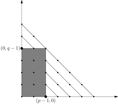
Figure 2. The case m=pq+1

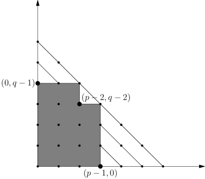
Figure 3. The case m=pq-1

Lemma 6.17.

If $k\geq{}2$ and $m>1$, then $\dim{}\mathsf{HP}_{0}(\mathcal{O}_{V}^{G},\mathcal{O}_{V})>\dim{}\mathsf{HH}_{0}(\mathcal{D}_{X}^{G},\mathcal{D}_{X})$.

The proof of this final lemma is long and somewhat technical, so we further subdivide it into several parts.

Proof.

Note that, by assumption, $p,q>1$. Write $m=bp+a$ for $0<a<p$ and $m=cq+d$ for $0<d<q$.

Claim 6.18.

$(a-1,b-1)$ and $(c-1,d-1)$ are corners of the staircase: $(a-1,b-1)$ is the rightmost before $(p-1,0)$, and $(c-1,d-1)$ is the leftmost after $(0,q-1)$, as in Figure 4.

Proof.

First, note that $b<q/k$ and $c<p/k$, since $m=\frac{pq\pm 1}{k}=bp+a=cq+d$. Next, for all $a^{\prime}$ such that $a<a^{\prime}<p$, $a^{\prime}+b^{\prime}p\equiv 0\pmod{m}$ implies that $b^{\prime}p>m$ so that $b^{\prime}>q/k$. Therefore, $(a^{\prime}-1,b^{\prime}-1)$ cannot be a corner of the staircase. It follows that $(a-1,b-1)$ is a corner. Similarly, if $d<d^{\prime}<q$, then $(c^{\prime}-1,d^{\prime}-1)$ cannot be a corner, and hence $(c-1,d-1)$ is a corner. ∎

In particular, it follows that $c\leq a$ and $d\geq b$ (see Figure 4). (A direct proof of this also follows from the argument of the proposition: first one shows $c<p/k$ and $b<q/k$; then if $a<c<p$, it would follow that $d>q/k$, a contradiction.) To summarize, $0<c\leq a<p$ and $0<b\leq d<q$.

Note also that $b=\lfloor{}\frac{m}{p}\rfloor{}=\lfloor{}\frac{q}{k}\rfloor{}$ and $c=\lfloor{}\frac{m}{q}\rfloor{}=\lfloor{}\frac{p}{k}\rfloor{}$. By our assumptions, $p,q<m/2$, and hence also $b,c\geq 2$.

Claim 6.19.

$p+b-2\leq{}m-p$.

Proof.

$$(m-p)-(p+b-2) =m+2-2p-b$$

$$\geq{}m+2-2p-\frac{m}{p}.$$

Let $f(p)=m+2-2p-\frac{m}{p}$. Since $f(p)$ is convex and $1<p<\frac{m}{2}$, it suffices to prove that $f(1)\geq 0$ and $f(\frac{m}{2})\geq 0$. This is clear because they are both $0$. ∎

Therefore, glancing at Figure 4, we see that there are chains beginning at $(p-1,0),\ldots,(p-1,b-2)$ of type (2) (in the language of the beginning of the section) which form connected components in $\mathcal{C}$. Similarly, there are chains of type (2) ending at $(0,q-1),\dotsc{},(c-2,q-1)$. Next, again from Figure 4, we see that there are points of type (1) of the form $(c-1,j)$ with $b-1\leq j<d-1$ and of the form $(i,b-1)$ for $c-1\leq i<a-1$, and also the chains $(c-1,d-1)$ and $(a-1,b-1)$ of type (2), each a connected component in $\mathcal{C}$ consisting of a single vertex (some of which may be equal). Together with the more obvious points $(i,j)$ of type (1) where either $i<c-1,j<q-1$ or $i<p-1,j<b-1$, we deduce

Claim 6.20.

$\dim{}\mathsf{HP}_{0}(\mathcal{O}_{V}^{G},\mathcal{O}_{V})\geq{}p(b-1)+q(c-1)-(b-1)(c-1)+(d-b)+(a-c)+1$.

Let $h$ denote the difference $h:=\dim{}\mathsf{HP}_{0}(\mathcal{O}_{V}^{G},\mathcal{O}_{V})-\bigl{(}p(b-1)+q(c-1)-(b-1)(c-1)+(d-b)+(a-c)+1\bigr{)}$. In particular, $h$ is at least the number of chains of type (2) containing vertices $(j,k)$ such that $j+k>\max\{c+d-2,a+b-2\}$ and $j<p-1,k<q-1$. (The last condition ensures that these chains are not the ones beginning with any of the vertices $(p-1,0),\ldots,(p-1,b-2)$ or ending at any of the vertices $(0,q-1),\ldots,(c-2,q-1)$, which we already counted above.)

Figure 4. The staircase for $k\geq 2$

In view of the claim and the formula for $\dim{}\mathsf{HH}_{0}(\mathcal{D}_{X}^{G},\mathcal{D}_{X})$, we deduce that

$$\dim{}\mathsf{HP}_{0} (\mathcal{O}_{V}^{G},\mathcal{O}_{V})-\dim{}\mathsf{HH}_{0}(\mathcal{D}_{X}^{G},\mathcal{D}_{X})$$

$$=p(b-1)+q(c-1)-(b-1)(c-1)+(d-b)+(a-c)+1-(m-1)+h$$

$$=m-a-p+m-d-q-bc+b+c-1+d-b+a-c+1-m+1+h$$

$$=m+1-p-q-bc+h.$$

We will need one more inequality which gives a lower bound on $p$, and similarly on $q$.

Claim 6.21.

$p\geq{}kc+1$. Similarly, $q\geq kb+1$.

Proof.

$pq\geq{}km-1=k(cq+d)-1>kcq$. The same argument shows $q>kb$. ∎

We now divide the lemma into five cases. In each case, we prove that $m+1-p-q-bc+h>0$. Up to symmetry (swapping $r$ with $t$), we will assume that $b\geq c$.

Case 1. $k=2$. Note that, since $b,c\geq 2$ as remarked at the beginning of the proof of the lemma, it follows that $p\geq kc+1\geq 5$ and similarly $q\geq 5$.

Case 1a. $m=\frac{pq-1}{2}$.

In this case, the staircase has three corners with nonnegative coefficients: $(p-1,0)$, $(\frac{p-1}{2}-1,\frac{q-1}{2}-1)$, and $(0,q-1)$. So $a=c=\frac{p-1}{2}$ and $b=d=\frac{q-1}{2}$. Then,

$$m+1-p-q-bc =\frac{pq-1}{2}+1-p-q-\frac{p-1}{2}\cdot\frac{q-1}{2}$$

$$=\frac{1}{4}(pq-3p-3q+1).$$

In addition, since $p,q\geq 5$, we have at least two additional chains in $\mathcal{C}$ of type (2): $(\frac{p-3}{2},\frac{q-1}{2}),(\frac{p-1}{2},\frac{q-3}{2})$ and $(\frac{p-3}{2},\frac{q+1}{2}),(\frac{p-1}{2},\frac{q-1}{2}),(\frac{p+1}{2},\frac{q-3}{2})$. So $h\geq 2$, and it suffices to prove that $pq-3p-3q+9=(p-3)(q-3)>0$, which is obvious.

Case 1b. $m=\frac{pq+1}{2}$.

In this case, the staircase has four corners with nonnegative coefficients: $(0,q-1)$, $(\frac{p-1}{2}-1,\frac{q+1}{2}-1)$, $(\frac{p+1}{2}-1,\frac{q-1}{2}-1)$, and $(0,p-1)$. So $a=\frac{p+1}{2}$, $b=\frac{q-1}{2}$, $c=\frac{p-1}{2}$, $d=\frac{q+1}{2}$. Then,

$$m+1-p-q-bc =\frac{pq+1}{2}+1-p-q-\frac{p-1}{2}\cdot\frac{q-1}{2}$$

$$=\frac{1}{4}(pq-3p-3q+5).$$

Also, since $p,q\geq 5$, there is at least one additional chain of type (2) in $\mathcal{C}$: $(\frac{p-3}{2},\frac{q+1}{2}),(\frac{p-1}{2},\frac{q-1}{2}),(\frac{p+1}{2},\frac{q-3}{2})$. So $h\geq 1$, and it suffices to prove that $pq-3p-3q+9>0$, which we already saw in Case 1a.

Case 2. $k\geq{}3$, $b\geq{}3$, $c\geq{}3$.

In this case, $m+1-p-q-bc>0$ follows from the inequalities

$$p <\frac{m}{b}\leq{}\frac{m}{3},$$

$$q <\frac{m}{c}\leq{}\frac{m}{3},\text{ and }$$

$$bc =\frac{m-a}{p}\cdot\frac{m-d}{q}<\frac{m^{2}}{pq}\leq{}\frac{m\frac{pq+1}{k}}{pq}=\frac{m}{k}+\frac{m}{kpq}<\frac{m}{3}+1.$$

Case 3. $k\geq{}3$, $c=2$, $b\geq{}4$.

Since $p\geq{}kc+1\geq{}7$,

$$p <\frac{m}{b}\leq{}\frac{m}{4},$$

$$q+\frac{1}{2}b \leq{}q+\frac{d}{2}=\frac{m}{2},\text{ and }$$

$$\frac{3}{2}b <\frac{3m}{2p}\leq{}\frac{3m}{14}.$$

For the inequality on the second line, see Figure 4 and the discussion after Claim 6.18. We deduce from the three lines that $m+1-p-q-bc=m+1-p-(q+\frac{1}{2}b)-(\frac{3}{2}b)>0$.

Case 4. $k\geq{}3$, $c=2$, $b=3$.

Note that $d\geq b=3$ and $a\geq c=2$. Hence

$$q =\frac{m-d}{c}\leq{}\frac{m-3}{2}\text{ and }$$

$$p =\frac{m-a}{b}\leq{}\frac{m-2}{3}.$$

So, $m-p-q-5\geq{}\frac{m-17}{6}$. Since $m>bp>bkc\geq{}18$, we conclude that $m-p-q-5>0$, as desired.

Case 5. $k\geq{}3$, $c=2$, $b=2$. Note that

$$m+1-p-q-bc =m+1-\frac{m-a}{2}-\frac{m-d}{2}-4$$

$$=\frac{a+d-6}{2}$$

Therefore, it suffices to prove that $2h+a+d>6$.

Case 5a. $a=d=2$.

In this case, we have at least two additional chains of type (2) in $\mathcal{C}$: $(1,2),(2,1)$ and $(1,3),(2,2),(3,1)$. Therefore, $h\geq 2$, as desired.

Case 5b. If we are not in the case $a=d=2$, then $(1,1)$ is not a corner of the staircase; in view of Figure 4, this implies $a,d>2$. It suffices to assume that $a=d=3$. We claim that this cannot happen. For sake of contradiction, assume $a=d=3$. Then, $m=2p+3=2q+3$. Since $m=\frac{pq\pm 1}{k}$, $4m$ divides $4(pq\pm 1)=m^{2}-6m+9\pm 4$. Therefore, $m$ is odd, so $m\mid m^{2}-6m+9\pm 4$, and hence $m$ divides $5$ or $13$. However, $m=2p+3\geq{}2(kc+1)+3\geq 17$, which is a contradiction. ∎

6.2.2. Case II: the general case

In this subsection, we complete the proof of Theorem 6.2 by reducing the general case to Proposition 6.14, which was proved in the previous subsection.

Lemma 6.22.

Let $A=\min\{r>0:x_{1}^{r}x_{2}^{s}\in\mathcal{O}_{V}^{G}\text{ or }x_{1}^{r}y_{2}^{s}\in\mathcal{O}_{V}^{G}\}$. Then, for every invariant of the form $x_{1}^{r}x_{2}^{s}$ or $x_{1}^{r}y_{2}^{s}$ in $\mathcal{O}_{V}^{G}$, $A\mid r$.

Proof.

It is enough to show the result for $r>0$. Suppose, for sake of contradiction, that $A\nmid r$ and $x_{1}^{r}x_{2}^{s}$ or $x_{1}^{r}y_{2}^{s}$ is an invariant. We can assume that $r$ is minimal for this property. There must exist $s^{\prime},s^{\prime\prime}\geq 0$ such that $x_{1}^{A}x_{2}^{s^{\prime}}$ and $x_{1}^{A}y_{2}^{s^{\prime\prime}}$ are invariants. In the first case that $x_{1}^{r}x_{2}^{s}$ is invariant, it follows also that $x_{1}^{r-A}x_{2}^{s+s^{\prime\prime}}$ is invariant; in the latter case that $x_{1}^{r}y_{2}^{s}$ is invariant, it follows also that $x_{1}^{r-A}y_{2}^{s+s^{\prime}}$ is invariant. This contradicts our assumption. ∎

Similarly, let $B=\min\{s>0:x_{1}^{r}x_{2}^{s}\in\mathcal{O}_{V}^{G}\text{ or }x_{1}^{r}y_{2}^{s}\in\mathcal{O}_{V}^{G}\}$. Then $B$ divides all of the $s$ appearing in the set. We construct a group $G^{\prime}$ in the following way:

$$G^{\prime}=\left\{\begin{pmatrix}\zeta^{A}&0\\ 0&\xi^{B}\end{pmatrix}:\begin{pmatrix}\zeta&0\\ 0&\xi\end{pmatrix}\in{}G\right\}.$$

Then $x_{1}^{Ar}x_{2}^{Bs}$ is an invariant of $G$ if and only if $x_{1}^{r}x_{2}^{s}$ is an invariant of $G^{\prime}$, and $x_{1}^{Ar}y_{2}^{Bs}$ is an invariant of $G$ if and only if $x_{1}^{r}y_{2}^{s}$ is an invariant of $G^{\prime}$.

Lemma 6.23.

$G=\left\{\begin{pmatrix}\zeta&0\\ 0&\xi\end{pmatrix}:\begin{pmatrix}\zeta^{A}&0\\ 0&\xi^{B}\end{pmatrix}\in{}G^{\prime}\right\}$.

Proof.

It is immediate from the above description that the two groups have the same invariants. This implies that the two groups are the same in a standard way: for example, if $G\leq H$ and $\mathcal{O}_{V}^{G}=\mathcal{O}_{V}^{H}$, then the quotient fields $\CC(V)^{G}$ and $\CC(V)^{H}$ would also be equal, and by the main theorem of Galois theory, $G=H$. ∎

Lemma 6.24.

$G^{\prime}$ is generated by $\begin{pmatrix}e^{2\pi{}i/m}&0\\ 0&e^{2r\pi{}i/m}\end{pmatrix}$, for some integers $r,m$ with $\mathrm{gcd}(r,m)=1$.

Proof.

Let $m\geq 1$ be the positive integer such that the first projection $\{\zeta:\begin{pmatrix}\zeta&0\\ 0&\xi\end{pmatrix}\in G^{\prime}\}$ is the cyclic group generated by $e^{2\pi i/m}$. By the definition of $G^{\prime}$, there exists $\ell\geq 1$ such that $x_{1}^{\ell}x_{2}\in\mathcal{O}_{V}^{G^{\prime}}$. It follows that the lattice $(\mathbb{Z}^{2})^{G^{\prime}}:=\{(a,b)\in\mathbb{Z}^{2}\mid x_{1}^{a}x_{2}^{b}\in\CC(V)^{G^{\prime}}\}$ is generated by $(m,0)$ and $(\ell,1)$. By assumption, $\mathrm{gcd}(\ell,m)=1$. Thus, we can let $r:=-\ell$, and then $(\mathbb{Z}^{2})^{G^{\prime}}$ identifies with the lattice invariant under the element stated in the lemma. This implies that $G^{\prime}$ is generated by the element. In more detail, if $K\leq G^{\prime}$ is the subgroup generated by this element, then $|K|=|\mathbb{Z}^{2}/(\mathbb{Z}^{2})^{K}|=|\mathbb{Z}^{2}/(\mathbb{Z}^{2})^{G^{\prime}}|=|G^{\prime}|$. ∎

We see that Case I of Theorem 6.2, i.e., Proposition 6.14, is equivalent to the case $A=B=1$. We divide the remainder of the theorem into two cases:

Case 1. $A,B>1$. In the case that $G^{\prime}$ is the trivial group, $G$ is evidently of the type (3) in Theorem 6.2, and it is easy to see that, for this group, $\dim\mathsf{HP}_{0}(\mathcal{O}_{V}^{G},\mathcal{O}_{V})=(A-1)(B-1)=\dim\mathsf{HH}_{0}(\mathcal{D}_{X}^{G},\mathcal{D}_{X})$. See also Figure 5.

Claim 6.25.

If $A,B>1$, and $G^{\prime}$ is nontrivial, then $\dim{}\mathsf{HP}_{0}(\mathcal{O}_{V}^{G},\mathcal{O}_{V})>\dim{}\mathsf{HH}_{0}(\mathcal{D}_{X}^{G},\mathcal{D}_{X})$.

Proof.

Without loss of generality, assume that $A\geq{}B$. Then $\dim{}\mathsf{HH}_{0}(\mathcal{D}_{X}^{G},\mathcal{D}_{X})=ABm-A-B+1$. Then, we prove that $\dim{}\mathsf{HP}_{0}(\mathcal{O}_{V}^{G},\mathcal{O}_{V})\geq{}AB\dim{}\mathsf{HP}_{0}(\mathcal{O}_{V}^{G^{\prime}},\mathcal{O}_{V})+2(A-1)(B-1)$ by the following correspondence:

(i) Let $(a,b)$ be a point that forms a connected component of $\Gamma(G^{\prime})$ of type (1). Then, for every $(r,s)\in E(G)$, either $a<r/A-1$ or $b<s/B-1$. Hence, $(Aa+i,Bb+j)$ forms a connected component of $\Gamma(G)$ of type (1) for each $0\leq{}i<A$, $0\leq{}j<B$, because $Aa+i<r-1$ or $bB+j<s-1$ for all $(r,s)\in E(G)$.

(ii) Let $(a,b+c),(a+1,b+c-1),\ldots,(a+c,b)$ form a connected component of $\Gamma(G^{\prime})$ of type (2). Then we can verify that $(Aa+i,B(b+c)+j)$ is a connected component of $\Gamma(G)$ of type (1) for each $0\leq{}i<A-1$, $0\leq{}j<B$, and that the chains starting from $(Aa+A-1,B(b+c)+j)$, $0\leq{}j<B$ are connected components of $\Gamma(G)$ of type (2).

(iii) In addition, each point $(A(m-1)+i,j)$ and $(i,B(m-1)+j)$, $0\leq{}i<A-1$, $0\leq{}j<B-1$ forms a connected component of $\Gamma(G)$ of type (1).

Thus, $\dim{}\mathsf{HP}_{0}(\mathcal{O}_{V}^{G},\mathcal{O}_{V})\geq{}AB\dim{}\mathsf{HP}_{0}(\mathcal{O}_{V}^{G^{\prime}},\mathcal{O}_{V})+2(A-1)(B-1)\geq{}AB(m-1)+2(A-1)(B-1)>ABm-A-B+1=\dim{}\mathsf{HH}_{0}(\mathcal{D}_{X}^{G},\mathcal{D}_{X})$. ∎

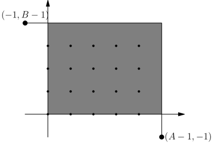
Figure 5. The staircase for type (3) in Theorem 6.2

Case 2. $A>1,B=1$ or $A=1,B>1$. Without loss of generality, assume that $A>1,B=1$.

Claim 6.26.

If $A>1$ and $B=1$, $G$ is nontrivial, and $\dim{}\mathsf{HP}_{0}(\mathcal{O}_{V}^{G},\mathcal{O}_{V})=\dim{}\mathsf{HH}_{0}(\mathcal{D}_{X}^{G},\mathcal{D}_{X})$, then $G^{\prime}$ is generated by $\begin{pmatrix}e^{2\pi{}i/m}&0\\ 0&e^{\pm{}2\pi{}i/m}\end{pmatrix}$.

For $G^{\prime}$ as in the claim, Lemma 6.23 implies that $G$ is generated by $\begin{pmatrix}e^{\pm{}2\pi{}i/(mA)}&0\\ 0&e^{2\pi{}i/m}\end{pmatrix}$. This accounts for the groups of type (2) in Theorem 6.2; conversely, it is an easy consequence of Theorem 6.5 that all of these groups indeed satisfy $\dim{}\mathsf{HP}_{0}(\mathcal{O}_{V}^{G},\mathcal{O}_{V})=\dim{}\mathsf{HH}_{0}(\mathcal{D}_{X}^{G},\mathcal{D}_{X})$. See also Figure 6. This finishes the proof of the theorem, and it remains only to prove the claim.

Proof of Claim 6.26.

Similarly to (i) and (ii) in Case 1 above,

$$\dim{}\mathsf{HH}_{0}(\mathcal{D}_{X}^{G},\mathcal{D}_{X})=A(m-1)=A\dim{}\mathsf{HH}_{0}(\mathcal{D}_{X}^{G^{\prime}},\mathcal{D}_{X})\text{ and }$$

$$\dim{}\mathsf{HP}_{0}(\mathcal{O}_{V}^{G},\mathcal{O}_{V})\geq{}A\dim{}\mathsf{HP}_{0}(\mathcal{O}_{V}^{G^{\prime}},\mathcal{O}_{V}).$$

Assume that $\dim{}\mathsf{HP}_{0}(\mathcal{O}_{V}^{G},\mathcal{O}_{V})=\dim{}\mathsf{HH}_{0}(\mathcal{D}_{X}^{G},\mathcal{D}_{X})$. Then, we must have $\dim{}\mathsf{HP}_{0}(\mathcal{O}_{V}^{G^{\prime}},\mathcal{O}_{V})=\dim{}\mathsf{HH}_{0}(\mathcal{D}_{X}^{G^{\prime}},\mathcal{D}_{X})$.

Define $p,q$ in the same way as in Case I (note that we must have $k=0$ or $k=1$). Then $(0,q-1)$ is the corner of the staircase for $G^{\prime}$ with $x$-coordinate equal to zero. This implies that the staircase for $G$ has the corner $(A-1,q-1)$. However, in this case, it would follow, similarly to the argument in Case 1 of this subsection, that $\dim\mathsf{HP}_{0}(\mathcal{O}_{V}^{G},\mathcal{O}_{V})>A\dim\mathsf{HP}_{0}(\mathcal{O}_{V}^{G^{\prime}},\mathcal{O}_{V})$ unless $q=1$. In the latter case, $G^{\prime}$ is as claimed. ∎

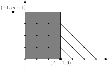
Figure 6. The staircase for type (2) in Theorem 6.2

7. Complex reflection groups $G(m,p,2)<\mathsf{GL}_{2}<\Sp_{4}$

Assume $m\geq 2$. Up to conjugation, the complex reflection group $G=G(m,p,2)<\mathsf{GL}_{2}$ has the form

(7.1) $$G=\biggl{\langle}\begin{pmatrix}e^{2\pi i/m}&0\\ 0&e^{-2\pi i/m}\end{pmatrix},\begin{pmatrix}e^{2\pi pi/m}&0\\ 0&1\end{pmatrix},\begin{pmatrix}0&1\\ 1&0\end{pmatrix}\biggr{\rangle}.$$

Let $K<G$ be the index-two abelian subgroup of diagonal matrices. As before, let $V=\CC^{4}$ and consider $K<G<\Sp(V)$ in the standard way. Let $r:=m/p$. Then, the invariants $\mathcal{O}_{V}^{K}$ are spanned by the monomials

(7.2) $$x_{1}^{a}x_{2}^{b}y_{1}^{c}y_{2}^{d},\quad m\mid\bigl{(}(a-c)-(b-d)\bigr{)},r\mid a,b,c,d.$$

The invariants $\mathcal{O}_{V}^{G}$ are spanned by the sums $x_{1}^{a}x_{2}^{b}y_{1}^{c}y_{2}^{d}+x_{1}^{b}x_{2}^{a}y_{1}^{d}y_{2}^{c}$ where $a,b,c$, and $d$ are as above. It follows easily that, as an algebra, $\mathcal{O}_{V}^{G}$ is generated by

(7.3) $$x_{1}y_{1}+x_{2}y_{2},x_{1}y_{1}x_{2}y_{2},x_{1}^{m}+x_{2}^{m},y_{1}^{m}+y_{2}^{m},x_{1}^{r}x_{2}^{r},y_{1}^{r}y_{2}^{r},x_{1}^{jr}y_{2}^{m-jr}+x_{2}^{jr}y_{1}^{m-jr}(1\leq j<p),$$

(7.4) $$x_{1}^{m+1}y_{1}+x_{2}^{m+1}y_{2},y_{1}^{m+1}x_{1}+y_{2}^{m+1}x_{2},x_{1}^{jr+1}y_{1}y_{2}^{m-jr}+x_{2}^{jr+1}y_{2}y_{1}^{m-jr}(1\leq j<p).$$

The second line consists of elements obtainable from those in the first line by a linear combination of bracketing with $x_{1}y_{1}x_{2}y_{2}$ and multiplying by $x_{1}y_{1}+x_{2}y_{2}$, and hence the first line Poisson generates $\mathcal{O}_{V}^{G}$. Therefore, $\{\mathcal{O}_{V}^{G},\mathcal{O}_{V}\}$ is spanned by $\{f,\mathcal{O}_{V}\}$ where $f$ ranges among the elements listed in (7.3).

In the next subsections we will consider separately the cases $p=1$, $p=m$, and $1<p<m$. We first consider $p=1$ since the computations here will be used in subsequent subsections as well.

Remark 7.5.

The techniques used here might also be able to handle the case of somewhat more general finite subgroups of $\mathsf{GL}_{2}$: namely, those generated by a subgroup of diagonal matrices together with an off-diagonal element with zeros on the diagonal. For such groups, we can use the subgroup $K<G$ of diagonal matrices, which has index two, and for which $\mathsf{HP}_{0}(\mathcal{O}_{V}^{K},\mathcal{O}_{V})$ was computed in the previous section. In more detail, there is a natural map $\mathsf{HP}_{0}(\mathcal{O}_{V}^{G})\hookrightarrow\mathsf{HP}_{0}(\mathcal{O}_{V}^{G},\mathcal{O}_{V})\twoheadrightarrow\mathsf{HP}_{0}(\mathcal{O}_{V}^{K},\mathcal{O}_{V})=\mathsf{HP}_{0}(\mathcal{O}_{V}^{K})$ whose image is $\mathsf{HP}_{0}(\mathcal{O}_{V}^{K})^{G}$, the part symmetric under swapping indices $1$ and $2$. The dimension of the latter is roughly $\frac{1}{2}\dim\mathsf{HP}_{0}(\mathcal{O}_{V}^{K})$, so estimates using Theorem 6.5, in the spirit of the previous section, should suffice to show that $\mathsf{HP}_{0}(\mathcal{O}_{V}^{G})\ncong\operatorname{\mathsf{gr}}\mathsf{HH}_{0}(\mathcal{D}_{X}^{G})$ for many of these $G$.

7.1. The case $p=1$

Set $G=G(m,1,2)$.

Theorem 7.6.

For $G=G(m,1,2)$, $\mathsf{HP}_{0}(\mathcal{O}_{V}^{G},\mathcal{O}_{V})\cong\operatorname{\mathsf{gr}}\mathsf{HH}_{0}(\mathcal{D}_{X}^{G},\mathcal{D}_{X})$, and a homogeneous basis for the former is given by the images of the elements

(7.7) $$x_{1}^{a}x_{2}^{b}y_{1}^{a}y_{2}^{b}\quad(a,b\leq m-2);\quad\quad x_{1}^{m-1}x_{2}^{a}y_{1}^{m-1}y_{2}^{a}+x_{1}^{a}x_{2}^{m-1}y_{1}^{a}y_{2}^{m-1}(1\leq a\leq m-1);$$

(7.8) $$x_{1}^{a+b}y_{1}^{a}y_{2}^{b},\quad x_{2}^{a+b}y_{1}^{b}y_{2}^{a}\quad(a+b\leq m-2,\,b\geq 1);$$

(7.9) $$bx_{1}^{m-1}y_{1}^{m-1-b}y_{2}^{b}-(m-b)x_{2}^{m-1}y_{1}^{m-b}y_{2}^{b-1}\quad(1\leq b\leq m-1).$$

The $G$-graded structure of $H=\mathsf{HP}_{0}(\mathcal{O}_{V}^{G},\mathcal{O}_{V})\cong\operatorname{\mathsf{gr}}\mathsf{HH}_{0}(\mathcal{D}_{X}^{G},\mathcal{D}_{X})$ follows immediately from (7.7)–(7.9). We will need some notation for the irreducible representations of $G$. Let $\chi$ be the tautological one-dimensional representation of the group of $m$-th roots of unity $\{e^{2\pi ki/m}\}$. For $0\leq a\leq m-1$, let $\rho_{a}:=\chi^{a}\circ\det$, so that $\rho_{0}$ is the trivial representation. Let $\rho_{0}^{-}$ be the nontrivial one-dimensional representation which restricts to the trivial representation on $K$, i.e., which is $-1$ on off-diagonal elements and $1$ on diagonal elements. Then, let $\rho_{a}^{-}:=\rho_{0}^{-}\otimes\rho_{a}$. Next, for $a\neq b$, let $\tau_{a,b}$ be the two-dimensional irreducible representation which restricts to $(\chi^{a}\boxtimes\chi^{b})\oplus(\chi^{b}\boxtimes\chi^{a})$ on $K$. There are ${m\choose 2}$ distinct such irreducible representations. Note that the corresponding representation in the case $a=b$ is $\rho_{a}\oplus\rho_{a}^{-}$.

Corollary 7.10.

(7.11) $$h(\text{Hom}_{G}(\rho_{0},H);t)=\sum_{j=0}^{m-2}\lfloor\frac{j+2}{2}\rfloor t^{2j}+\sum_{j=m-1}^{2m-4}\lfloor\frac{2m-2-j}{2}\rfloor t^{2j}+\sum_{j=0}^{m-2}t^{2m+2j};$$

(7.12) $$h(\text{Hom}_{G}(\rho_{0}^{-},H);t)=\sum_{j=0}^{m-2}\lfloor\frac{j+1}{2}\rfloor t^{2j}+\sum_{j=m-1}^{2m-4}\lfloor\frac{2m-3-j}{2}\rfloor t^{2j};$$

(7.13) $$h(\text{Hom}_{G}(\tau_{b,-b},H);t)=(t^{2b}+t^{2b+2}+\cdots+t^{2(m-b)-2})\\ +(2t^{2(m-b)}+2t^{2(m-b)+4}+\cdots+2t^{2m-4})+t^{2m-2},\quad 1\leq b<m/2;$$

If $m$ is odd, then for all other irreducible representations $\rho$, $\text{Hom}_{G}(\rho,H)=0$. If $m$ is even, then this is true except for $\rho_{m/2}$ and $\rho_{m/2}^{-}$, for which

(7.14) $$h(\text{Hom}_{G}(\rho_{m/2},H);t)=t^{m}+t^{m+2}+\cdots+t^{2m-4};$$

(7.15) $$h(\text{Hom}_{G}(\rho_{m/2}^{-},H);t)=t^{m}+t^{m+2}+\cdots+t^{2m-2}.$$

We omit the proof of the corollary, since it follows directly from the theorem.

Proof of Theorem 7.6.

We will prove that the given elements map to a basis of $\mathsf{HP}_{0}(\mathcal{O}_{V}^{G},\mathcal{O}_{V})$. From this it is easy to deduce that $\mathsf{HP}_{0}(\mathcal{O}_{V}^{G},\mathcal{O}_{V})\cong\operatorname{\mathsf{gr}}\mathsf{HH}_{0}(\mathcal{D}_{X}^{G},\mathcal{D}_{X})$: we only need to compute that the dimensions are equal, since there is always a surjection. By Lemma 1.1, $\dim\mathsf{HH}_{0}(\mathcal{D}_{X}^{G},\mathcal{D}_{X})$ equals the number of elements $g\in G$ such that $g-\operatorname{Id}$ are invertible. There are $(m-1)^{2}$ diagonal elements without $1$ on the diagonal, and $m(m-1)$ off-diagonal matrices of determinant not equal to $-1$, and these are exactly the elements such that $g-\operatorname{Id}$ is invertible. So it is enough to show that $\dim\mathsf{HP}_{0}(\mathcal{O}_{V}^{G},\mathcal{O}_{V})=(m-1)(2m-1)$, and this follows by computing the number of basis elements.

We will compute explicitly the brackets of (7.3) and show that the claimed elements form a basis of $\mathsf{HP}_{0}(\mathcal{O}_{V}^{G},\mathcal{O}_{V})$. Since $p=1$, only the first four elements of (7.3) are needed. So, we compute the brackets with these elements.

First, $\{x_{1}y_{1}+x_{2}y_{2},\mathcal{O}_{V}^{G}\}$ is the span of all monomials $x_{1}^{a}x_{2}^{b}y_{1}^{c}y_{2}^{d}$ with $a+b\neq c+d$.

Next, $\{x_{1}y_{1}x_{2}y_{2},\mathcal{O}_{V}^{G}\}$ is the span of elements $(c-a)x_{1}^{a-1}x_{2}^{b}y_{1}^{c-1}y_{2}^{d}+(d-b)x_{1}^{a}x_{2}^{b-1}y_{1}^{c}y_{2}^{d-1}$. In the case $a+b=c+d$ (otherwise the monomial is in the span of the previous paragraph), this reduces to $x_{1}^{a-1}x_{2}^{b}y_{1}^{c-1}y_{2}^{d}+x_{1}^{a}x_{2}^{b-1}y_{1}^{c}y_{2}^{d-1}$. So if we quotient by this and the brackets of the previous paragraph, the result is spanned by the images of the monomials

(7.16) $$x_{1}^{a}x_{2}^{b}y_{1}^{a}y_{2}^{b}\quad(a,b\geq 0);\quad\quad x_{1}^{a+b}y_{1}^{a}y_{2}^{b},\quad x_{2}^{a+b}y_{1}^{b}y_{2}^{a}\quad(a\geq 0,b>0),$$

remembering also the equivalences

(7.17) $$x_{1}^{a+b}y_{1}^{a}y_{2}^{b}\equiv x_{1}^{a+b-c}x_{2}^{c}y_{1}^{a-c}y_{2}^{b+c},\quad x_{2}^{a+b}y_{1}^{b}y_{2}^{a}\equiv x_{1}^{c}x_{2}^{a+b-c}y_{1}^{b+c}y_{2}^{a-c},\quad\quad c\leq a,b>0,$$

which we will use for subsequent relations.

Finally, $\{x_{1}^{m}+x_{2}^{m},\mathcal{O}_{V}^{G}\}$ is spanned by $cx_{1}^{a+m-1}x_{2}^{b}y_{1}^{c-1}y_{2}^{d}+dx_{1}^{a}x_{2}^{b+m-1}y_{1}^{c}y_{2}^{d-1}$, and similarly for $\{y_{1}^{m}+y_{2}^{m},\mathcal{O}_{V}^{G}\}$. In particular, this includes the elements $x_{1}^{a}x_{2}^{b}y_{1}^{a+b}$ and $x_{1}^{b}x_{2}^{a}y_{2}^{a+b}$ for $a\geq m-1$ and $b\geq 0$. Together with the spans described in the previous paragraphs, we can first restrict our attention to the case $a+b+m-1=c+d-1$, i.e., $d=a+b-c+m$. Then, we obtain the monomials of the second two forms of (7.16) in the case that $a\geq m-1$, i.e.,

(7.18) $$x_{1}^{a+b}y_{1}^{a}y_{2}^{b},\quad x_{2}^{a+b}y_{1}^{b}y_{2}^{a}\quad(a\geq m-1,b>0).$$

The remaining elements in the span yield, up to the symmetry of swapping $x_{1}$ with $x_{2}$ and $y_{1}$ with $y_{2}$ (and still assuming $d=a+b-c+m$),

$$cx_{1}^{a+b+m-1}y_{1}^{b+c-1}y_{2}^{d-b}+dx_{2}^{a+b+m-1}y_{1}^{c-a}y_{2}^{a+d-1},\quad\text{if $a<c,b<d$};$$

$$x_{1}^{a+b+m-1}y_{1}^{b+c-1}y_{2}^{d-b},\quad\text{if $a>c$};$$

(7.19) $$(b+m)x_{1}^{a}x_{2}^{b+m-1}y_{1}^{a}y_{2}^{b+m-1}+ax_{1}^{a+b+m-1}y_{1}^{a+b-1}y_{2}^{m},\quad\text{if $a=c$}.$$

The final expression (7.19) together with (7.18) yields the first monomial of (7.19) when $a+b\geq m$, or equivalently (by changing $a$ and $b$):

(7.20) $$x_{1}^{a}x_{2}^{b}y_{1}^{a}y_{2}^{b},\quad a+b\geq 2m-1.$$

The expressions in the two lines above (7.19) can be rewritten, by changing $a,b,c,d$, as

$$cx_{1}^{a+b}y_{1}^{a}y_{2}^{b}+(a+b+1-c)x_{2}^{a+b}y_{1}^{m-b}y_{2}^{a+2b-m}\quad(0<m-b\leq c\leq a+1,\,b>0);$$

(7.21) $$x_{1}^{a+b}y_{1}^{a}y_{2}^{b},\quad x_{2}^{a+b}y_{1}^{b}y_{2}^{a}\quad(b>m).$$

For fixed $a$ and $b$, if there is more than one possible value of $c$ in the first equation above, then in fact both monomials that appear are in the span. So, we can rewrite this as

(7.22) $$(a+1)x_{1}^{m-1}y_{1}^{a}y_{2}^{m-a-1}+(m-a-1)x_{2}^{m-1}y_{1}^{a+1}y_{2}^{m-a-2}\quad(a<m-1);$$

(7.23) $$x_{1}^{a+b}y_{1}^{a}y_{2}^{b},\quad x_{2}^{a+b}y_{1}^{b}y_{2}^{a}\quad(a+b\geq m,\,0<b<m).$$

Applying the aforementioned swap of indices $1$ and $2$ to (7.19), we also obtain

(7.24) $$(b+m)x_{1}^{b+m-1}x_{2}^{a}y_{1}^{b+m-1}y_{2}^{a}+ax_{2}^{a+b+m-1}y_{1}^{m}y_{2}^{a+b-1}.$$

The overall span (7.18)–(7.24) is now symmetric in swapping indices $1$ and $2$. It is also almost symmetric in swapping $x$ with $y$ using (7.17), since the latter shows that $x_{1}^{a+b}y_{1}^{a}y_{2}^{b}$ is equivalent to $x_{1}^{b}x_{2}^{a}y_{2}^{a+b}$ when $b>0$. However, (7.19) yields, after swapping $x$ with $y$ and applying (7.17),

$$(b+m)x_{1}^{a}x_{2}^{b+m-1}y_{1}^{a}y_{2}^{b+m-1}+ax_{2}^{a+b+m-1}y_{1}^{m}y_{2}^{a+b-1}.$$

Up to (7.24), this is equivalent to

(7.25) $$x_{1}^{a}x_{2}^{b+m-1}y_{1}^{a}y_{2}^{b+m-1}-x_{1}^{b+m-1}x_{2}^{a}y_{1}^{b+m-1}y_{2}^{a}.$$

We conclude that $\mathsf{HP}_{0}(\mathcal{O}_{V}^{G},\mathcal{O}_{V})$ is presented as the span of monomials (7.16) modulo span of (7.18)–(7.25). From this the statement of the theorem easily follows. ∎

7.2. The case $p=m$, i.e., the Coxeter groups $I_{2}(m)$

In the case $p=m$, $G(m,m,2)$ is the Coxeter group $I_{2}(m)$.

Theorem 7.26.

If $p=m$, then $\mathsf{HP}_{0}(\mathcal{O}_{V}^{G},\mathcal{O}_{V})\cong\operatorname{\mathsf{gr}}\mathsf{HH}_{0}(\mathcal{O}_{V}^{G},\mathcal{O}_{V})$, and a homogeneous basis of the former is given by the images of the elements

(7.27) $$x_{1}^{a}y_{1}^{a}+(-1)^{a}x_{2}^{a}y_{2}^{a},0\leq a\leq m-2.$$

We can immediately deduce the graded $G$-structure. Let $\rho_{0}$ be the trivial representation and “$\det$” the determinant representation. Let $H:=\mathsf{HP}_{0}(\mathcal{O}_{V}^{G},\mathcal{O}_{V})\cong\operatorname{\mathsf{gr}}\mathsf{HH}_{0}(\mathcal{O}_{V}^{G},\mathcal{O}_{V})$.

Corollary 7.28.

(7.29) $$h(\text{Hom}_{G}(\rho_{0},H);t)=1+t^{4}+\cdots+t^{4\lfloor\frac{m-2}{2}\rfloor}\text{ and }h(\text{Hom}_{G}(\det,H);t)=t^{2}+t^{6}+\cdots+t^{4\lfloor\frac{m-1}{2}\rfloor-2}.$$

Proof of Theorem 7.26.

As in the proof of Theorem 7.6, it is enough to prove that the claimed elements form a basis of $\mathsf{HP}_{0}(\mathcal{O}_{V}^{G},\mathcal{O}_{V})$, since there are $m-1$ basis elements and this equals the number of elements $g\in G$ such that $g-\operatorname{Id}$ is invertible (in this case, they are the nontrivial diagonal elements of $G$).

To do this, we compute explicitly the remaining brackets of (7.3) needed. In this case, the final element of (7.3) is unnecessary, since it is a scalar multiple of the bracket $\{x_{1}x_{2},y_{1}^{m}+y_{2}^{m}\}$. So, $\mathsf{HP}_{0}(\mathcal{O}_{V}^{G},\mathcal{O}_{V})$ is the quotient of the span of (7.16) and also the equivalent monomials according to (7.17), modulo (7.18)–(7.25) together with the span of $\{x_{1}x_{2},\mathcal{O}_{V}\}+\{y_{1}y_{2},\mathcal{O}_{V}\}$. We now compute these spans.

Note that

(7.30) $$\{x_{1}x_{2},x_{1}^{a}x_{2}^{b}y_{1}^{c}y_{2}^{d}\}=cx_{1}^{a}x_{2}^{b+1}y_{1}^{c-1}y_{2}^{d}+dx_{1}^{a+1}x_{2}^{b}y_{1}^{c}y_{2}^{d-1}.$$

In the case $c=0$ or $d=0$ but not both, this yields the monomial $x_{1}^{a}x_{2}^{b+1}y_{1}^{c-1}$ or $x_{1}^{a+1}x_{2}^{b}y_{2}^{d-1}$. Applying this to the span $\{y_{1}y_{2},\mathcal{O}_{V}\}$ and changing the $a,b,c$, and $d$, we obtain the monomials

(7.31) $$x_{1}^{c}y_{1}^{a}y_{2}^{b},\quad x_{2}^{c}y_{1}^{b}y_{2}^{a},\quad\quad b\geq 1.$$

This already includes all but the first type of monomial in (7.16). For the remaining type, let us assume $a=c-1$ and $b+1=d$ in (7.30). Then we obtain the element

(7.32) $$(a+1)x_{1}^{a}x_{2}^{b+1}y_{1}^{a}y_{2}^{b+1}+(b+1)x_{1}^{a+1}x_{2}^{b}y_{1}^{a+1}y_{2}^{b}.$$

By symmetry, this is the end of the new elements of $\{\mathcal{O}_{V}^{G},\mathcal{O}_{V}\}$ added in the case $p=m$ to those (7.18)–(7.25) from the previous section. Note that (7.19) and (7.24) together with (7.31) yields

(7.33) $$x_{1}^{a}x_{2}^{b}y_{1}^{a}y_{2}^{b},\quad\text{$a\geq m-1$ or $b\geq m-1$}.$$

Now, putting (7.31)–(7.33) together, applied to the monomials (7.16) modulo (7.17), we can recover all of the elements (7.18)–(7.25), and we easily deduce the statement of the theorem. ∎

7.3. The case $1<p<m$

Theorem 7.34.

If $G=G(m,p,n)<\mathsf{GL}_{2}<\Sp_{4}$ and $1<p<m$, then a basis of $\mathsf{HP}_{0}(\mathcal{O}_{V}^{G},\mathcal{O}_{V})$ is obtained by the images of the elements

(7.35) $$x_{1}^{a}x_{2}^{b}y_{1}^{a}y_{2}^{b},\quad a<r-1,b<m-1\text{ or }a<m-1,b<r-1;$$

(7.36) $$x_{1}^{a}x_{2}^{r-1}y_{1}^{a}y_{2}^{r-1}+(-1)^{a-r+1}x_{1}^{r-1}x_{2}^{a}y_{1}^{r-1}y_{2}^{a},\quad r-1\leq a\leq m-r-1;$$

(7.37) $$x_{1}x_{2}^{m-1}y_{1}y_{2}^{m-1}+x_{1}^{m-1}x_{2}y_{1}^{m-1}y_{2},\quad p=2;$$

(7.38) $$x_{1}^{a+b}y_{1}^{a}y_{2}^{b},\quad x_{2}^{a+b}y_{1}^{b}y_{2}^{a},\quad\quad b>0,(\text{either }a+b<2r-1\text{ or }a<r-1),\text{ and:}$$

$$\text{$\nexists k\in[b,a+b]$ s.t.~{}both $\lfloor\frac{k+1}{r}\rfloor+\lfloor\frac{a+2b-k}{r}\rfloor\geq p$}\text{ and }k\neq m/2-1;$$

(7.39) $$x_{1}^{a+b}y_{1}^{a}y_{2}^{b}+x_{2}^{a+b}y_{1}^{b}y_{2}^{a},\quad b>0,(\text{either $a+b<2r-1$ or $a<r-1$}),$$

$$a+2b\geq m,\text{ and }\lfloor\frac{a+b+1}{r}\rfloor=p/2;$$

(7.40) $$x_{1}^{a+b}y_{1}^{a}y_{2}^{b}-x_{2}^{a+b}y_{1}^{b}y_{2}^{a},\quad\frac{a+b+1}{r}=\frac{p+1}{2},\quad\frac{b}{r}>\frac{p-1}{2}.$$

We remark that the condition of (7.38) in particular implies $a+b<m-1$ (by taking $k=a+b\geq m-1$), so it is consistent with Theorem 7.6, noting that $\mathsf{HP}_{0}(\mathcal{O}_{V}^{G},\mathcal{O}_{V})$ for $G=G(m,p,2)$ is a quotient of $\mathsf{HP}_{0}(\mathcal{O}_{V}^{H},\mathcal{O}_{V})$ for $H=G(m,1,2)>G$.

Also, note that the statement of the theorem actually holds when $p=m>2$, and reduces to Theorem 7.26, but since the result is then much simpler, we separated the two theorems.

Corollary 7.41.

For $1<p<m$, $\mathsf{HP}_{0}(\mathcal{O}_{V}^{G},\mathcal{O}_{V})\ncong\operatorname{\mathsf{gr}}\mathsf{HH}_{0}(\mathcal{D}_{X}^{G},\mathcal{D}_{X})$. Also, $\mathsf{HP}_{0}(\mathcal{O}_{V}^{G})\ncong\operatorname{\mathsf{gr}}\mathsf{HH}_{0}(\mathcal{D}_{X}^{G})$ unless $p=2$ and $m\in\{4,6\}$, in which case one obtains

(7.42) $$h(\mathsf{HP}_{0}(\mathcal{O}_{V}^{G});t)=h(\operatorname{\mathsf{gr}}\mathsf{HH}_{0}(\mathcal{D}_{X}^{G});t)=1+t^{2}+3t^{4}+t^{8},\quad G=G(4,2,2);$$

(7.43) $$h(\mathsf{HP}_{0}(\mathcal{O}_{V}^{G});t)=h(\operatorname{\mathsf{gr}}\mathsf{HH}_{0}(\mathcal{D}_{X}^{G});t)=1+t^{2}+2t^{4}+3t^{6}+4t^{8}+t^{10}+t^{12},\quad G=G(6,2,2).$$

In general, when $1<p<m$,

(7.44) $$h(\mathsf{HP}_{0}(\mathcal{O}_{V}^{G});t)=\sum_{j=0}^{2r-5}\lfloor\frac{j+2}{2}\rfloor t^{2j}+\sum_{j=2r-4}^{m-2}(r-1)t^{2j}+\sum_{j=m-1}^{m+r-4}(m+r-3-j)t^{2j}\\ +\sum_{j=0}^{\lfloor\frac{m-2r}{2}\rfloor}t^{4(r+j-1)}+\delta_{p,2}t^{2m}+\delta_{2\mid p}\sum_{i=0}^{r-2}t^{m+2i},$$

where $\delta_{2\mid p}=1$ if $p$ is even and $\delta_{2\mid p}=0$ otherwise.

It is also possible to use Theorem 7.34 to give an explicit description of the graded $G$-structure of $\mathsf{HP}_{0}(\mathcal{O}_{V}^{G},\mathcal{O}_{V})$ similarly to Corollaries 7.10 and 7.28, but we omit this as it is complicated and less explicit. In computing the Hilbert series of the $G$-invariants above, the relevant basis elements above greatly simplify.

Remark 7.45.

As a consequence of the theorem, we see that, for $1<p<m$, the top degree of $\mathsf{HP}_{0}(\mathcal{O}_{V},\mathcal{O}_{V}^{G})$ is the same as the top degree of $\mathsf{HP}_{0}(\mathcal{O}_{V}^{G})$, which is $2(m+r-4)$ except in the cases $p=2$ and $m\in\{4,6\}$ (exactly the same cases wherein $\mathsf{HP}_{0}(\mathcal{O}_{V}^{G})\cong\operatorname{\mathsf{gr}}\mathsf{HH}_{0}(\mathcal{O}_{V}^{G})$), in which case the top degree is $2m$. In contrast, Theorem 7.6 shows that, in the case $p=1$, the top degree is $4m-4$, which is also the same as the top degree of $G$-invariants; Theorem 7.26 shows that, in the case $p=m$ (i.e., the Coxeter groups of type $I_{2}(m)$), the top degree is $2m-4$, while the top degree of $G$-invariants is either $2m-4$ or $2m-6$, whichever is a multiple of $4$. In the case $m$ is odd, these produce some of the only examples of groups considered in this paper such that the top degree of $\mathsf{HP}_{0}(\mathcal{O}_{V}^{G},\mathcal{O}_{V})$ exceeds that of $\mathsf{HP}_{0}(\mathcal{O}_{V}^{G})$: the other examples are the groups $S_{n+1}<\mathsf{GL}_{n}<\Sp_{2n}$ (i.e., the type $A_{n}$ Weyl groups). This does not include groups mentioned for which we did not actually compute $\mathsf{HP}_{0}(\mathcal{O}_{V}^{G},\mathcal{O}_{V})$, such as complex reflection groups of rank $\geq 3$ and $G_{18}$ and $G_{19}$.

Finally, note that the actual top degrees for $G(m,p,2)$ above differ from the bounds of Corollary 3.9 (assuming $m>1$): there we have $2m+4r-8$, whereas the actual top degree as above is a constant plus $2m+2r$ (the constant depending on whether $p=1,p=m$, or $1<p<m$, with the special cases $(m,p)\in\{(4,2),(6,2)\}$). The only cases where the bound is sharp are $p=m$, $(m,p)=(4,2)$, and $(m,p)=(2,2)$.

7.3.1. Proof of Theorem 7.34

We need to compute the spans of brackets with the final three elements of (7.3), when summed with the spans already computed from §7.1.

First, $\{x_{1}^{r}x_{2}^{r},x_{1}^{a}x_{2}^{b}y_{1}^{c}y_{2}^{d}\}=crx_{1}^{a+r-1}x_{2}^{b+r}y_{1}^{c-1}y_{2}^{d}+drx_{1}^{a+r}x_{2}^{b+r-1}y_{1}^{c}y_{2}^{d-1}$. Together with the similar expression for brackets with $y_{1}^{r}y_{2}^{r}$, and up to (7.17), this yields the span of

(7.46) $$(a+1)x_{1}^{a}x_{2}^{b+1}y_{1}^{a}y_{2}^{b+1}+(b+1)x_{1}^{a+1}x_{2}^{b}y_{1}^{a+1}y_{2}^{b},\quad a,b\geq r-1;$$

(7.47) $$x_{1}^{a+b}y_{1}^{a}y_{2}^{b},x_{2}^{a+b}y_{1}^{b}y_{2}^{a},\quad a+b\geq 2r-1,a\geq r-1,b>0.$$

Together with (7.19), since $m\geq 2r$, this also yields

(7.48) $$x_{1}^{a}x_{2}^{b}y_{1}^{a}y_{2}^{b},\quad a+b\geq r+m-1.$$

It remains to consider the final element of (7.3) (note that $m-jr=(p-j)r$):

(7.49) $$\{x_{1}^{jr}y_{2}^{m-jr}+x_{2}^{jr}y_{1}^{m-jr},x_{1}^{a}x_{2}^{b}y_{1}^{c}y_{2}^{d}\}=r\Bigl{[}\bigl{(}jcx_{1}^{a+jr-1}x_{2}^{b}y_{1}^{c-1}y_{2}^{d+m-jr}-(p-j)bx_{1}^{a+jr}x_{2}^{b-1}y_{1}^{c}y_{2}^{d+m-jr-1}\bigr{)}\\ -\bigl{(}(p-j)ax_{1}^{a-1}x_{2}^{b+jr}y_{1}^{c+m-jr-1}y_{2}^{d}-jdx_{1}^{a}x_{2}^{b+jr-1}y_{1}^{c+m-jr}y_{2}^{d-1}\bigr{)}\Bigr{]}$$

We will assume that $(a+jr-1)+b=c-1+(d+m-jr)$, since otherwise the above is all in the span of $\{x_{1}y_{1}+x_{2}y_{2},\mathcal{O}_{V}^{G}\}$ as noted in §7.1.

In the case $a+jr=c$, so that the first two terms on the RHS have the form $x_{1}^{a^{\prime}}x_{2}^{b^{\prime}}y_{1}^{a^{\prime}}y_{2}^{b^{\prime}}$, we can simplify the above using (7.46). We can restrict our attention to the case that $a+d<r$, since otherwise all the terms on the RHS are already in the span of (7.47) and (7.48), using also the relations (7.17). Then, up to the previous spans and rescaling we obtain

(7.50) $$p(a+jr)x_{1}^{a+jr-1}x_{2}^{d+m-jr}y_{1}^{a+jr-1}y_{2}^{d+m-jr}-((p-j)a-jd)x_{2}^{a+d+m-1}y_{1}^{m}y_{2}^{a+d-1}.$$

In the case $a=d=0$, the second term vanishes and we obtain the monomial $x_{1}^{jr-1}x_{2}^{m-jr}y_{1}^{jr-1}y_{2}^{m-jr}$ in the span. Otherwise, substituting (7.24), this is equivalent to

(7.51) $$(a+d)p(a+jr)x_{1}^{a+jr-1}x_{2}^{d+m-jr}y_{1}^{a+jr-1}y_{2}^{d+m-jr}+m((p-j)a-jd)x_{1}^{a+d}x_{2}^{m-1}y_{1}^{a+d}y_{2}^{m-1}.$$

If, instead of $a+jr=c$, we have $b+jr=d$, i.e., the second two terms on the RHS of (7.49) have the form $x_{1}^{a^{\prime}}x_{2}^{b^{\prime}}y_{1}^{a^{\prime}}y_{2}^{b^{\prime}}$ (rather than the first two terms), then up to (7.25) and swapping $j$ with $p-j$, we obtain the same relations.

Let analyze (7.50) and (7.51) further. Using (7.51) together with (7.46) (and the case $a=d=0$ of (7.50)), we can replace all monomials of the form $x_{1}^{a}x_{2}^{b}y_{1}^{a}y_{2}^{b}$ for $a,b\geq r-1$ and $a+b\geq m-1$ by monomials of the form $x_{1}^{a+b-m+1}x_{2}^{m-1}y_{1}^{a+b-m+1}y_{2}^{m-1}$ as above. It remains to see when two such ways, for fixed $a$ and $b$, are irredundant, and hence $x_{1}^{a+b-m+1}x_{2}^{m-1}y_{1}^{a+b-m+1}y_{2}^{m-1}$ is itself in the span. We already saw that the latter is true when $a+b=m-1$, by (7.19).

In the case that $a=0$ and $d=1$ of (7.50), then (7.51) becomes, after dividing by $mj$,

(7.52) $$x_{1}^{jr-1}x_{2}^{m-jr+1}y_{1}^{jr-1}y_{2}^{m-jr+1}-x_{1}x_{2}^{m-1}y_{1}x_{2}^{m-1}.$$

In the case that $a=1$ and $d=0$ of (7.50), applying also (7.46), we obtain

$$-\frac{jr}{m-jr+1}p(1+jr)x_{1}^{jr-1}x_{2}^{m-jr+1}y_{1}^{jr-1}y_{2}^{m-jr+1}+m(p-j)x_{1}x_{2}^{m-1}y_{1}y_{2}^{m-1}.$$

Together with (7.52), this yields both monomials above, and in particular $x_{1}x_{2}^{m-1}y_{1}x_{2}^{m-1}$, unless $jrp(1+jr)=m(p-j)(m-jr+1)$. Substituting $m=pr$ this equality becomes $\frac{j}{p-j}=\frac{(p-j)r+1}{jr+1}$. This holds if and only if $j=p-j$: if $j\neq p-j$, then one is strictly between both sides. Note further that, unless $p=2$, then we can always choose $j$ so that $j\neq p-j$, and therefore we obtain the monomial $x_{1}x_{2}^{m-1}y_{1}y_{2}^{m-1}$ in the span.

In the case that $a+d>1$, then (7.51) can be applied to at least three pairs $(a,d)$ with the same sum, and it is easy to see that the second monomial (which does not change) must be in the span, and hence all the monomials which appear are in the span. To summarize, (7.49) yields, in the case $c=a+jr$,

(7.53) $$x_{1}^{a}x_{2}^{m-1}y_{1}^{a}y_{2}^{m-1},a\geq 2\text{ or }a=1,p>2.$$

In the remaining case of (7.49) where neither $a+jr=c$ nor $b+jr=d$, provided $c,d\geq 1$, using (7.17), (7.49) becomes

(7.54) $$(jc-(p-j)b)x_{1}^{a+jr-1}x_{2}^{b}y_{1}^{c-1}y_{2}^{d+m-jr}-((p-j)a-jd)x_{1}^{a}x_{2}^{b+jr-1}y_{1}^{c+m-jr}y_{2}^{d-1}.$$

As before, we assume that the total degree in $x_{1}$ and $x_{2}$ equals the total degree in $y_{1}$ and $y_{2}$, i.e., $a+b+jr=c+d+m-jr$. In particular, $a+b\equiv c+d\pmod{r}$.

If $c=0$ and/or $d=0$, then we instead get the same relation as above, except that we must multiply the first term above by $\frac{x_{1}y_{1}}{x_{2}y_{2}}$ and/or the second term by $\frac{x_{2}y_{2}}{x_{1}y_{1}}$, respectively. (Note that if $b=c=0$ then the first term is zero, and if $a=d=0$ then the second term is zero.)

The first term above vanishes if and only if $jc=(p-j)b$, and the second term if and only if $jd=(p-j)a$. One way the first equality can hold is if $b=c=0$, in which case the second monomial appearing above is in the overall span unless $jd=(p-j)a$, in which case we obtain no relations. If $b+c=1$, then the first term does not vanish, and we obtain a nontrivial relation. If $b+c>1$ and either $a,c>0$ or $b,d>0$, then we can replace $(a,b,c,d)$ by $(a\pm 1,b\mp 1,c\pm 1,d\mp 1)$, and together with (7.17), the new expression (7.54) is irredundant unless $j=p-j$.

The same arguments apply if we swap $b$ and $c$ with $a$ and $d$. So, all the monomials that can occur above are actually in the span, unless we are in one of the cases $b+c=1=a+d$, one of $a,c$ and one of $b,d$ are zero, or $j=p-j$ and $b+c,a+d>0$. Even if we are in one of these cases, by applying also (7.17), we can still obtain the first monomial in the span if $b+c\geq r$, and the second monomial in the span if $a+d\geq r$. We can therefore discard the case $b+c=1=a+d$, since this together with $b+c<r$ and $a+d<r$ already implies $j=p-j$.

Next, let us assume that $b+c<r$ and $a+d<r$, in addition to being in one of the two cases (i) one of $a,c$ and one of $b,d$ are zero, or (ii) $j=p-j$ and $b+c,a+d>0$. Then, applying again (7.17), we obtain a single nontrivial relation unless either $a=d=0$ and $jc=(p-j)b$ are both satisfied or $b=c=0$ and $jd=(p-j)a$ are both satisfied. Then, we are in case (i), so $j=p-j$, and either (1) both $a=d=0$ and $b=c<r$ are satisfied, or (2) both $a=d<r$ and $b=c=0$ are satisfied. So, in these final two subcases (1) and (2) only, (7.54) yields no relations on the monomials (7.16) modulo (7.17), and otherwise we obtain a single nontrivial relation.

Putting everything together, one may verify that (7.54) adds to the overall span of $\{\mathcal{O}_{V}^{G},\mathcal{O}_{V}\}$ exactly the following:

(7.55) $$x_{1}^{a+b}y_{1}^{a}y_{2}^{b},\quad b>0,\,\lfloor\frac{a+b+1}{r}\rfloor\neq p/2,\frac{a+b+1}{r}\neq\frac{p+1}{2},\text{ and }$$

$$\exists k\in[b,a+b]\text{ s.t. }\lfloor\frac{k+1}{r}\rfloor+\lfloor\frac{a+2b-k}{r}\rfloor\geq p;$$

(7.56) $$x_{1}^{a+b}y_{1}^{a}y_{2}^{b}-x_{2}^{a+b}y_{1}^{b}y_{2}^{a},\quad b>0,\lfloor\frac{a+b+1}{r}\rfloor=p/2,a+2b\geq m;$$

(7.57) $$x_{1}^{a+b}y_{1}^{a}y_{2}^{b}+x_{2}^{a+b}y_{1}^{b}y_{2}^{a},\quad\frac{a+b+1}{r}=\frac{p+1}{2},\quad\frac{b}{r}>\frac{p-1}{2}.$$

Therefore, $\mathsf{HP}_{0}(\mathcal{O}_{V}^{G},\mathcal{O}_{V})$ is the quotient of the span of monomials (7.16) up to (7.17) and the relations (7.46)–(7.48), (7.53), and (7.55)–(7.57). From this, we easily obtain the basis claimed in the theorem. (A priori, we might also need to include relations from §7.1, but it is easy to see they are all spanned by the present relations, by comparing the basis of the present theorem with that of Theorem 7.6. Alternatively, one can verify directly that the aforementioned relations span also (7.18)–(7.25). This completes the proof of Theorem 7.34.

7.3.2. Proof of Corollary 7.41

First, to prove (7.44), we can use the basis of the theorem: it is easy to see that the dimension of the space of $G$-invariants in each degree is the number of terms of the form $x_{1}^{a}x_{2}^{b}y_{1}^{a}y_{2}^{b}+x_{1}^{b}x_{2}^{a}y_{1}^{b}y_{2}^{a}$ and, in the case $p$ is even, also $x_{1}^{a+m/2}y_{1}^{a}y_{2}^{m/2}+x_{2}^{a+m/2}y_{1}^{m/2}y_{1}^{a}$, which are in the span of the elements appearing in the theorem. From this (7.44) easily follows.

Now, (7.44) implies that the LHS and RHS of (7.42) are equal by substituting in the given values of $m$ and $p$, and similarly for (7.43). To deduce from this that $\mathsf{HP}_{0}(\mathcal{O}_{V}^{G})\cong\operatorname{\mathsf{gr}}\mathsf{HH}_{0}(\mathcal{D}_{X}^{G})$ in the cases $p=2$ and $m\in\{4,6\}$, and hence the equality with the second term in the these two equations, it suffices to show that $\dim\mathsf{HP}_{0}(\mathcal{O}_{V}^{G})=\dim\mathsf{HH}_{0}(\mathcal{D}_{X}^{G})$. By Lemma 1.1, $\dim\mathsf{HH}_{0}(\mathcal{D}_{X}^{G},\mathcal{D}_{X})$ and $\dim\mathsf{HH}_{0}(\mathcal{D}_{X}^{G})$ equal the number of elements $g\in G$ such that $g-\operatorname{Id}$ is invertible and the number of conjugacy classes of such elements, respectively. First, there are $(m-r)r+(r-1)^{2}$ diagonal matrices in $G$ without $1$ on the diagonal; of these there are $r-1$ or $2r-1$ scalar matrices, depending on whether $p$ is odd or even, respectively. The diagonal matrices with distinct diagonal entries appear in conjugacy classes of size two. Next, the off-diagonal matrices $g$ such that $g-\operatorname{Id}$ is invertible are those of determinant not equal to $-1$, i.e., equal to a nontrivial $r$-th root of unity. There are $m(r-1)$ of these. Their conjugacy classes are of size either $m$ (in the case $p$ is odd) or $m/2$ (in the case $p$ is even). Putting this together, we conclude

(7.58) $$\dim\mathsf{HH}_{0}(\mathcal{D}_{X}^{G},\mathcal{D}_{X})=(2r-1)(m-1),$$

(7.59) $$\dim\mathsf{HH}_{0}(\mathcal{D}_{X}^{G})=\begin{cases}\frac{1}{2}r(m+1)-1,&\text{$p$ is odd},\\ \frac{1}{2}r(m+4)-2,&\text{$p$ is even}.\end{cases}$$

We easily deduce from this and (7.42) and (7.43) the fact that $\dim\mathsf{HH}_{0}(\mathcal{D}_{X}^{G})=\dim\mathsf{HP}_{0}(\mathcal{O}_{V}^{G})$ in these cases. Moreover, using (7.58) and an explicit calculation from the basis given in the theorem, or using computer programs from Magma, we see that $\dim\mathsf{HP}_{0}(\mathcal{O}_{V}^{G},\mathcal{O}_{V})>\dim\mathsf{HH}_{0}(\mathcal{D}_{X}^{G},\mathcal{D}_{X})$ in these cases: for $(m,p)=(4,2)$, we obtain dimensions $12>9$, and in the case $(m,p)=(6,2)$, we obtain dimensions $34>25$.

It remains to prove that, in all other cases (i.e., other than $p=2$ and $m\in\{4,6\}$) $1<p<m$ implies that $\mathsf{HP}_{0}(\mathcal{O}_{V}^{G})\not\cong\operatorname{\mathsf{gr}}\mathsf{HH}_{0}(\mathcal{D}_{X}^{G})$, since this clearly implies $\mathsf{HP}_{0}(\mathcal{O}_{V}^{G},\mathcal{O}_{V})\ncong\operatorname{\mathsf{gr}}\mathsf{HH}_{0}(\mathcal{D}_{X}^{G},\mathcal{D}_{X})$. For this, it suffices to show that $\dim\mathsf{HP}_{0}(\mathcal{O}_{V}^{G})>\dim\mathsf{HH}_{0}(\mathcal{D}_{X}^{G})$. From (7.44) we can easily compute $\dim\mathsf{HP}_{0}(\mathcal{O}_{V}^{G})$ by plugging in $t=1$; or we can compute it from the theorem itself and the observations of the first paragraph of the proof. The first line becomes the number of elements of the form $x_{1}^{a}x_{2}^{b}y_{1}^{a}y_{2}^{b}+x_{1}^{b}x_{2}^{a}y_{1}^{b}y_{2}^{a}$ with $a\leq b\leq m-2$ and $a\leq r-2$, which is the area of an obvious trapezoid in the plane: $(r-1)(m-1)-\frac{1}{2}(r-1)(r-2)$. The evaluation of the second line of (7.44) at $t=1$ is $\delta_{p,2}+\lfloor\frac{m-2r}{2}\rfloor+1+(r-1)\delta_{2\mid p}$. Put together,

(7.60) $$\dim\mathsf{HP}_{0}(\mathcal{O}_{V}^{G})=(r-1)(m-\frac{1}{2}r)+\lfloor\frac{m-2r}{2}\rfloor+(r-1)\delta_{2\mid p}+1+\delta_{p,2}.$$

Since the value of the formula in (7.59) for the even case of $p$ exceeds that of the odd case, let us subtract the even case formula from (7.60) and try to see when the result is positive. We get:

(7.61) $$(\frac{1}{2}r-1)(m-r-5)+\lfloor\frac{(p-2)r}{2}\rfloor+(r-1)\delta_{2\mid p}-2+\delta_{p,2}.$$

All of the terms above except for the first sum to a nonnegative number unless $p=3$ and $r=2$. The first term will be positive whenever $r>2$ and $(p-1)r>5$; the second condition is satisfied for all pairs $(p,r)$ with $r>2$ except when $p=2$ and $r\in\{3,4,5\}$. It remains to check these last cases (along with $r=2$).

If $r=2$, then the above sum is positive unless either $p=2$ or $p=3$. If $p=2$ and $r\in\{3,4,5\}$, then the above is clearly positive unless $r=3$. So this leaves only the cases $(p,r)\in\{(2,2),(2,3),(3,2)\}$. The first two cases are those in which the above is zero and we actually get $\mathsf{HP}_{0}(\mathcal{O}_{V}^{G})\cong\operatorname{\mathsf{gr}}\mathsf{HH}_{0}(\mathcal{D}_{X}^{G})$. In the final case $p=3,r=2$, $\dim\mathsf{HP}_{0}(\mathcal{O}_{V}^{G})=7>6=\dim\mathsf{HH}_{0}(\mathcal{D}_{X}^{G})$ (recall that (7.61) used the formula (7.59) in the case $p$ is even). This completes the proof.

Appendix A Examples where $\mathsf{HP}_{0}(\mathcal{O}_{V}^{G})$ is nontrivial in cubic degree

Let $G$ be a group and $V_{1},V_{2}$, and $V_{3}$ three quaternionic irreducible representations: then $(\operatorname{\mathsf{Sym}}^{2}V_{i})^{G}=0$ for all $i\in\{1,2,3\}$. If, furthermore, $(V_{i}\otimes V_{j})^{G}=0$ for all $i\neq j$ and $(V_{1}\otimes V_{2}\otimes V_{3})^{G}\neq 0$, then it would follow that the lowest degree invariant element in $\mathcal{O}_{V_{1}\oplus V_{2}\oplus V_{3}}^{G}$ is cubic. Equipping $V:=V_{1}\oplus V_{2}\oplus V_{3}$ with a $G$-invariant symplectic form, $\mathsf{HP}_{0}(\mathcal{O}_{V}^{G})$ would have a nontrivial cubic component, isomorphic to the cubic part of $\mathcal{O}_{V}^{G}$ itself. Our goal is to construct such $G,V_{1},V_{2}$, and $V_{3}$.

To do so, we will employ the field ${\mathbb{F}}_{2}$ and the Arf invariant. Let $m\geq 1$ and let $E$ be a ${\mathbb{F}}_{2}$-vector space of dimension $2m$. Let $Q_{E}$ denote the group of quadratic forms on $E$ with values in ${\mathbb{F}}_{2}$. Corresponding to each $q\in Q_{E}$ is a canonical central extension $\widetilde{E}_{q}$ of $E$ by ${\mathbb{F}}_{2}$, since $H^{2}(E,{\mathbb{F}}_{2})=Q_{E}$. If $q$ is nondegenerate, then it is well known [Dic07, Arf41] that $(E,q)$ is isomorphic to either $U_{0}^{m}$ or $U_{0}^{m-1}\oplus U_{1}$, where $U_{0}$ and $U_{1}$ are defined as ${\mathbb{F}}_{2}^{2}$ with the quadratic forms $x_{1}x_{2}$ and $x_{1}^{2}+x_{1}x_{2}+x_{2}^{2}$, respectively. In the former case, $q$ is said to have Arf invariant $0$, and in the latter case, Arf invariant $1$; the Arf invariant is the value that $q$ attains on the majority of vectors.

It follows that, if $q$ is nondegenerate, then $\widetilde{E}_{q}$ has a (unique) irreducible representation $Y_{q}$ of dimension $2^{m}$ (note that any such irreducible representation must be unique and of maximal dimension, since $|\widetilde{E}_{q}|=2^{2m+1}$ equals the sum of squares of dimensions of the irreducible representations). Namely, if $q=q_{1}\oplus\cdots\oplus q_{m}$, then $\widetilde{E}_{q_{1}\oplus\cdots\oplus q_{m}}$ is a central quotient of $\prod_{i}\widetilde{E}_{q_{i}}$, and $Y_{q}=Y_{q_{1}}\boxtimes\cdots\boxtimes Y_{q_{m}}$. This reduces one to the case $m=1$, where the central extensions corresponding to $U_{0}$ and $U_{1}$ are just the dihedral and quaternion groups of order eight, each equipped with a (unique) irreducible $2$-dimensional representation. It also follows that $Y_{q}$ is equipped with a canonical $\widetilde{E}_{q}$-invariant bilinear form, which is symmetric or skew-symmetric, depending on whether the Arf invariant of $q$ is $0$ or $1$, respectively (since this is true in the case $m=1$). That is, $Y_{q}$ is real or quaternionic, respectively.

Next, there is a canonical group which puts together all the central extensions for varying $q$: Let $Q_{E}$ be the ${\mathbb{F}}_{2}$-vector space of quadratic forms on $E$. Then $H^{2}(E,{\mathbb{F}}_{2})=Q_{E}$ and so there is a canonical element of $H^{2}(E,Q_{E}^{*})$ yielding a central extension

$$1\to Q_{E}^{*}\to G\to E\to 1.$$

Then, $G$ also acts on $Y_{q}$ with action factoring through $\widetilde{E}_{q}$, which is the pushout of the above extension under the evaluation map $q:Q_{E}^{*}\to{\mathbb{F}}_{2}$. It follows that $Y_{q}$ is an irreducible representation of $G$ that is real or quaternionic, depending on whether the Arf invariant of $q$ is $0$ or $1$, respectively. Moreover, for distinct nondegenerate quadratic forms $q_{1},q_{2}$, $Y_{q_{1}}\ncong Y_{q_{2}}$. Furthermore, one may check that, if $q_{1}+q_{2}$ is nondegenerate, then $Y_{q_{1}}\otimes Y_{q_{2}}\cong Y_{q_{1}+q_{2}}^{2^{m}}$.

Now, suppose that we are given quadratic forms $q_{1}$ and $q_{2}$ of Arf invariant $1$ such that $q_{1}+q_{2}$ is nondegenerate and also has Arf invariant $1$. Then, setting $q_{3}:=q_{1}+q_{2}$, we deduce that $(\operatorname{\mathsf{Sym}}^{2}Y_{q_{i}})^{G}=0$ and $(Y_{q_{i}}\otimes Y_{q_{j}})^{G}=0$ for all $i\neq j$, but since $q_{1}+q_{2}=q_{3}$, $(Y_{q_{1}}\otimes Y_{q_{2}}\otimes Y_{q_{3}})^{G}\neq 0$. Thus, $G,Y_{q_{1}},Y_{q_{2}}$, and $Y_{q_{1}+q_{2}}$ provide an example of the desired form. In fact, in this case, setting $V:=Y_{q_{1}}\oplus Y_{q_{2}}\oplus Y_{q_{3}}$, the cubic part of $\operatorname{\mathsf{Sym}}(\mathcal{O}_{V}^{G})$ and hence $\mathsf{HP}_{0}(\mathcal{O}_{V}^{G})$ is isomorphic to $(Y_{q_{1}}\otimes Y_{q_{2}}\otimes Y_{q_{3}})^{G}$, which is $2^{m}$-dimensional.

It is not hard to find such examples. Using Magma we found several with $m=2$ (the minimum possible value), such as $q_{1}=x_{1}x_{2}+x_{3}^{2}+x_{3}x_{4}+x_{4}^{2}$ and $q_{2}=x_{1}^{2}+x_{1}x_{4}+x_{2}^{2}+x_{2}x_{3}+x_{3}x_{4}$. In this case, setting $V:=Y_{q_{1}}\oplus Y_{q_{2}}\oplus Y_{q_{1}+q_{2}}$, the space $\mathsf{HP}_{0}(\mathcal{O}_{V}^{G})$ is nonzero in cubic degree (where it has dimension four), and $\dim V=12$.

References

- [AFLS00] J. Alev, M. A. Farinati, T. Lambre, and A. L. Solotar, Homologie des invariants d’une algèbre de Weyl sous l’action d’un groupe fini, J. Algebra 232 (2000), 564–577.
- [AL98] J. Alev and T. Lambre, Comparaison de l’homologie de Hochschild et de l’homologie de Poisson pour une déformation des surfaces de Klein, Algebra and operator theory (Tashkent, 1997) (Dordrecht), Kluwer Acad. Publ., 1998, pp. 25–38.
- [Arf41] C. Arf, Untersuchungen über quadratischen formen in körpern der charakteristik 2, i, J. Reine Angew. Math. 183 (1941), 148–167.
- [BCP97] W. Bosma, J. Cannon, and C. Playoust, The Magma algebra system. I. The user language, J. Symbolic Comput. 24 (1997), no. 3–4, 235–265.
- [BEG04] Y. Berest, P. Etingof, and V. Ginzburg, Morita equivalence of Cherednik algebras, J. Reine Angew. Math. 568 (2004), 81–98, arXiv:math/0207295.
- [BMR98] Michel Broué, Gunter Malle, and Raphaël Rouquier, Complex reflection groups, braid groups, Hecke algebras, J. Reine Angew. Math. 500 (1998), 127–190.
- [But09] F. Butin, Poisson homology in degree 0 for some rings of symplectic invariants, J. Algebra 322 (2009), no. 10, 3580–3613, arXiv:0809.4983.
- [Dic07] L. E. Dickson, Linear groups with an exposition of the galois field theory, New York: Cosimo Classics, 2007, Originally published 1901.
- [EG02] P. Etingof and V. Ginzburg, Symplectic reflection algebras, Calogero-Moser space, and deformed Harish-Chandra homomorphism, Invent. Math. 147 (2002), no. 2, 243–348.
- [EG07] P. Etingof and V. Ginzburg, Noncommutative del Pezzo surfaces and Calabi-Yau algebras, arXiv:0709.3593v4, 2007.
- [Eis95] D. Eisenbud, Commutative algebra with a view towards algebraic geometry, GTM 150, Springer Verlag, 1995.
- [ES] P. Etingof and T. Schedler, Poisson traces for symmetric powers of symplectic varieties and reflection representations of Weyl groups, in preparation.
- [ES09a] by same author, Poisson traces and -modules on Poisson varieties, arXiv:0908.3868, with an appendix by I. Losev, 2009.
- [ES09b] by same author, Zeroth Poisson homology of symmetric powers of quasihomogeneous isolated surface singularities, arXiv:0907.1715, 2009.
- [Mat95] O. Mathieu, The symplectic operad, Functional analysis on the eve of the 21st century, Vol. 1 (New Brunswick, NJ, 1993) (Boston, MA), Progr. Math., vol. 131, Birkhäuser Boston, 1995, pp. 223–243.
- [RS10a] Q. Ren and T. Schedler, On the asymptotic -structure of invariant differential operators on symplectic manifolds, arXiv:1006.0268, 2010.
- [RS10b] by same author, Some Magma programs computing the zeroth Poisson homology of invariant functions on symplectic vector spaces, 2010, http://math.mit.edu/~trasched/hp0-progs/.
- [ST54] G. C. Shephard and J. A. Todd, Finite unitary reflection groups, Canadian J. Math. 6 (1954), 274–304.