A Complex Networks Approach for Data Clustering

Abstract

Many methods have been developed for data clustering, such as k-means, expectation maximization and algorithms based on graph theory. In this latter case, graphs are generally constructed by taking into account the Euclidian distance as a similarity measure, and partitioned using spectral methods. However, these methods are not accurate when the clusters are not well separated. In addition, it is not possible to automatically determine the number of clusters. These limitations can be overcome by taking into account network community identification algorithms. In this work, we propose a methodology for data clustering based on complex networks theory. We compare different metrics for quantifying the similarity between objects and take into account three community finding techniques. This approach is applied to two real-world databases and to two sets of artificially generated data. By comparing our method with traditional clustering approaches, we verify that the proximity measures given by the Chebyshev and Manhattan distances are the most suitable metrics to quantify the similarity between objects. In addition, the community identification method based on the greedy optimization provides the smallest misclassification rates.

I Introduction

Classification is one of the most intrinsic activities of human beings, being used to facilitate the handling and organization of the huge amount of information that we receive every day. As a matter of fact, the brain is able to recognize objects in scenes and also to provide a categorization of objects, persons, or events. This classification is performed in order to cluster objects that are similar with respect to common attributes. Actually, humans have by now classified almost all known living species and materials on earth. Due to the importance of the classification task, it is fundamental to develop methods able to perform this task automatically. Indeed, many methods for categorization have been developed with application to life sciences (biology, zoology), medical sciences (psychiatry, pathology), social sciences (sociology, archaeology), earth sciences (geography, geology), and engineering Anderberg (1973); Jain et al. (1999a).

The process of classification can be performed in two different ways, i.e. supervised classification, where the previously known class of objects are provided as prototypes for classifying additional objects; and unsupervised classification, where no previous knowledge about the classes is provided. In the latter case, the categorization is performed in order to maximize the similarity between the objects in each class while minimizing the similarity between objects in different classes. In the current work, we introduce a method for unsupervised classification based on complex networks.

Unsupervised classification may be found under different names in different contexts, such as clustering (in pattern recognition), numerical taxonomy (in ecology) and partition (in graph theory). In the current work, we adopt the term “clustering”. Clustering can be used in many tasks, such as data reduction, performed by grouping data into cluster and processing each cluster as a single entity; hypothesis generation, when there is no information about the analyzed data; hypothesis testing, i.e. verification of the validity of a particular hypothesis; and prediction based on classes, where the obtained clusters are based on the characteristics of the respective patterns. As a matter of fact, clustering is a fundamental tool for many research fields, such as machine learning, data mining, pattern recognition, image analysis, information retrieval, and bioinformatics Jain et al. (1999a); Everitt et al. (2001).

Many methods have been developed for data clustering Theodoridis and Koutroumbas (2003), many of which are based on graph theory Jain et al. (1999b). Graphs-based clustering methods take into account algorithms related to minimum spanning trees Zahn (2006), region of influence (e.g. Urquhart (1982)), direct trees Koontz et al. (2006) and spectral analysis Koontz et al. (2006). These methods are able to detect clusters of various shapes, at least for the case in which they are well separated. However, these algorithms present some drawbacks, such as the spectral clustering, which only divides the graph into two groups and not in an arbitrary number of clusters. Division into more than two groups can be achieved by repeated bisection, but there is no guarantee of reaching the best division into three groups Theodoridis and Koutroumbas (2003). Also, these methods give no hint about how many clusters should be identified. On the other hand, methods for community identification in networks are able to handle these drawbacks Newman and Girvan (2004). Moreover, these methods provide more accurate partitions than the traditional method based on graph, such as the spectral partition Newman and Girvan (2004). Actually, methods based on complex networks are improvements of clustering approaches based on graphs.

Only recently, a method has been developed for data clustering based on complex networks concepts de Oliveira et al. (2008). In this case, the authors proposed a clustering method based on graph partitioning and the Chameleon algorithm Karypis et al. (2002). Although this method is able to detect clusters in different shapes, it presents some drawbacks. The authors considered a method for community identification very particular which does not provide the most accurate network division Fortunato (2010). In addition, it considered only a single metric to establish the connections between every pair of objects, i.e. the Euclidian distance. On the other hand, the method introduced in the current work overcomes all these limitations. We adopt the most accurate community identification methods and use the most traditional metrics to define the similarity between objects, including the Euclidian, Manhattan, Chebyshev, Fu and Tanimoto distances Theodoridis and Koutroumbas (2003). The accuracy of our methodology is evaluated in artificial as well as two real-world databases. Moreover, we compare our methodology with some traditional clustering algorithms, i.e. k-means, cobweb, expectation maximization and farthest first. We verify that our approach provides the smallest error rates. So, we concluded that complex networks theory seems to provide the tools and concepts able to improve the clustering methods based on graphs, potentially overcoming the most traditional clustering methods.

II Concepts and Methods

II.1 Complex networks

Complex networks are graphs with non-trivial topological features, whose connections are distributed as a power-law Albert and Barabási (2002). An undirected network can be represented by its adjacency matrix $A$, whose elements $a_{ij}$ are equal to one whenever there is a connection between the vertices $i$ and $j$, or equal to zero otherwise. A more general representation takes into account weighted connections, where each edge $(i,j)$ presents an associated weight or strength $\omega(i,j)$.

Different measures have been developed to characterize the topology of network structures, such as the clustering coefficient, distance-related measurements and centrality metrics da F. Costa et al. (2007). By allowing the different network properties to be quantified, these methods have revealed that most real-world networks are far from purely random Newman (2010).

In addition to this highly intricate topological organization, complex networks also tend to present modular structure. In this case, these modules are clusters whose vertices present similar roles, such as in the case of the brain of mammals, where cortical modules are associated to brain functions Bullmore and Sporns (2009). Communities have the same principle as clusters in pattern recognition research. In this way, the algorithms developed for community identification can also be used to partition graph and finding clusters.

Different methods have been developed in order to find communities in networks. Basically, these methods can be grouped as spectral methods (e.g. Newman (2006)), divisive methods (e.g. Girvan and Newman (2002)), agglomerative methods (e.g. Clauset et al. (2004)), and local methods (e.g. Clauset (2005)). The choice of the best method depends of the specific application, including the network size and number of connections. This is due to the fact that the most precise methods, such as the extremal optimization algorithm, are quite time expensive. Here, we take three different methods that provide accurate results, but have different time complexities. These methods are described in the next section.

The quality of a particular network division can be evaluated in terms of the modularity measure. This metric allows the number of communities to be automatically determined according to the best network partition. For a network partitioned into $m$ communities, a matrix $E$, $c\times c$, is constructed whose elements $e_{ij}$, represent the fraction of connections between communities $i$ and $j$. The modularity $Q$ is calculated as

$$Q=\sum_{i}[e_{ii}-(\sum_{j}e_{ij})^{2}]=\mathrm{Tr}E-||E^{2}||.$$ (1)

The highest value of modularity is obtained for the best network division. In particular, networks that present high values of $Q$ have modular structure implying that clusters are identified with high accuracy Newman and Girvan (2004); Newman (2010).

II.2 Clustering based on network

In literature, there are many definitions of clusters Theodoridis and Koutroumbas (2003), such as that provided by Everitt et al. Everitt et al. (2001), where clusters are understood as continuous regions of the feature space containing a high density of points, separated from other high density regions by low density regions. This definition is similar to that of network communities, i.e. a community is topologically defined as a subset of highly inter-connected vertices which are relatively sparsely connected to nodes in other communities Fortunato (2010).

Let each object (also denominated pattern) be represented by a feature vector $\vec{x}=[x_{1},x_{2},\ldots,x_{n}]$. These features, $x_{i}$, are scalar numbers and quantify the properties of objects. For instance, in case of the Iris database, the objects are flowers and the attributes are the length and the width of the sepal and the petal, in centimeters Fisher (1936). The clustering approach consists of grouping the feature vectors into $m$ clusters, $C_{1},C_{2},\ldots,C_{m}$, in such a way that objects belonging to the same cluster exhibit higher similarity with each other than with objects in other groups.

The process of clustering based on networks involves the definition of the following concepts:

1. Proximity measure: each object is represented as a node, where each pair of nodes are connected according to their similarity. These connections are weighted in the sense so as to quantify how similar each pair of vertices is, in terms of their feature vector. In this way, the most similar objects are connected by the strongest edges.

2. Clustering criterion: modularity is the most traditional measure used to quantify de quality of a network division Fortunato (2010), see Equation 1. Here, we adopt this metric to automatically choose the best cluster partition. In problems in which the number of clusters is known, it is not necessary to consider the modularity.

3. Clustering algorithms: Complex networks theory provides many algorithms for community identification, which act as the clustering algorithms Fortunato (2010). The choice of the most suitable method for a particular application should take into account the error rate and the execution time.

4. Validation of the results: The validation of the clustering methods based on networks can be performed in two different ways: (i) by considering databases in which the clusters are known (or at least expected), such as the Iris database Fisher (1936), and (ii) by taking into account artificial data with cluster organization, which allows to control the level of the data modular organization.

Proximity measures can be classified into two types, similarity measures, that is $s(\vec{x},\vec{y})=s_{0}$ only if $\vec{x}=\vec{y}$ and $-\infty<s(\vec{x},\vec{y})\leq s_{0}<+\infty$; and dissimilarity measures, where $d(\vec{x},\vec{y})=d_{0}$ only if $\vec{x}=\vec{y}$ and $-\infty<d_{0}\leq d(\vec{x},\vec{y})<+\infty$. To construct networks, it is more natural to adopt similarity measures, since it is expected that the edges with the strongest weights should be verified between the vertices with the most similar feature vectors. In this way, we adopt the following similarity measures to develop the network-based clustering approach Theodoridis and Koutroumbas (2003):

1. Inverse of Euclidian distance:

   $$D_{E}^{-1}(\textbf{x},\textbf{y})=\frac{1}{d_{2}(\textbf{x},\textbf{y})},$$ (2)

   where $d_{2}(\textbf{x},\textbf{y})$ is the traditional Euclidian distance. This metric results in values in the interval $[0,\infty)$.

2. Exponential of Euclidian distance:

   $$S_{E}(\textbf{x},\textbf{y})=\alpha\exp\left(-\alpha d_{2}(\textbf{x},\textbf{y})\right),$$ (3)

   where this metric results in values in the interval $[0,\alpha]$.

3. Inverse of Manhattan distance:

   $$D_{M}^{-1}(\textbf{x},\textbf{y})=\left(\sum_{i=1}^{n}|x_{i}-y_{i}|\right)^{-1},$$ (4)

   which assumes values in $[0,\infty)$.

4. Exponential of Manhattan distance:

   $$S_{M}(\textbf{x},\textbf{y})=\alpha\exp\left(-\alpha D_{M}\right),$$ (5)

   assuming values in the interval $[0,\alpha]$.

5. Inverse of Chebyshev distance:

   $$D_{C}^{-1}(\textbf{x},\textbf{y})=\frac{1}{\max_{i=1}^{n}|x_{i}-y_{i}|}.$$ (6)

   This metric results in values in $[0,\infty)$.

6. Exponential of Chebyshev distance:

   $$S_{C}(\textbf{x},\textbf{y})=\alpha\exp\left(-\alpha D_{C}\right),$$ (7)

   assuming values in the interval $[0,\alpha]$.

7. Metric proposed by Fu,

   $$F(\textbf{x},\textbf{y})=1-\frac{d_{2}(\textbf{x},\textbf{y})}{\parallel\textbf{x}\parallel+\parallel\textbf{y}\parallel}.$$ (8)

   This metrics results in values in the interval $[0,1]$

8. Exponential of the metric proposed by Fu:

   $$S_{F}(\textbf{x},\textbf{y})=\alpha\exp\left(-\alpha\frac{1-F}{2}\right).$$ (9)

   If $F(\textbf{x},\textbf{y})=1$, then $S_{F}(\textbf{x},\textbf{y})=\alpha$. If $F(\textbf{x},\textbf{y})=0$, then $S_{F}(\textbf{x},\textbf{y})=\alpha\exp\left(\frac{-\alpha}{2}\right)$. Therefore, $S_{F}$ assumes values in this limited interval.

9. Exponential of the Tanimoto mesure:

   $$S_{T}=\alpha\exp\left(-\alpha\frac{1-T}{2}\right),$$ (10)

   where

   $$T(\textbf{x},\textbf{y})=\frac{\textbf{x}^{T}\textbf{y}}{{\parallel\textbf{x}\parallel}^{2}+{\parallel\textbf{y}\parallel}^{2}-\textbf{x}^{T}\textbf{y}}.$$ (11)

   This metric assumes values in $(-\infty,1]$. Therefore, if $T(\textbf{x},\textbf{y})=1$, then, $s_{T}(\textbf{x},\textbf{y})=\alpha$, if $T(\textbf{x},\textbf{y})\rightarrow-\infty$, then, $S_{T}(\textbf{x},\textbf{y})\rightarrow 0$

In order to divide networks into communities and therefore obtain the clusters, we adopt three methods, namely the maximization of the modularity method, which is based on the greedy algorithm Clauset et al. (2004), here called fastgreedy algorithm; the extremal optimization approach Duch and Arenas (2005) and the waltrap method Pons and Latapy (2005). In both former methods, two communities $i$ and $j$ are joined according to the increase of the modularity $Q$ of the network. Thus, starting with each vertex disconnected and considering each of them as a community, we repeatedly join communities together into pairs, choosing at each step the merging that results in the greatest increase (or smallest decrease) of the modularity $Q$. The best division corresponds to the partition that resulted in the highest value of $Q$. The difference between these two methods lies in the choice of the optimization algorithm. On the other hand, the walktrap method is based on random walks, where the community identification uses a metrics that considers the probability transition matrix Pons and Latapy (2005). The time of execution of the walktrap method run as $O(N^{2}\log N)$. While the fastgreedy method is believed to be the fastest one, running in $O(N\log^{2}N)$, the extremal optimization provides the most accurate division Danon et al. (2005). On the other hand, the extremal optimization method is not particularly fast, scaling as $O(N^{2}\log N)$.

The validation of the network-based clustering method is performed with respect to artificial (i.e. computer generated clusters) and real-world databases. In the case of artificial data, we use two different configurations, i.e. (i) two separated clouds of points with a Gaussian distribution in a two dimensional space, and (ii) two semi-circles with varying density of points, as presented in Figure 1. In the former case, the validation set consists of two set of points (clusters) generated according to a gaussian distribution with covariance matrix equals to identity, ($\Sigma=I$). The median of one set of points is moved from the origin $(0,0)$ until (0,15), in steps of 0.75, while the other cluster remains fixed at the origin of axis. In this way, the distance between clusters is varied from $d=0$ to $d=15$. Figure 1(a) to (c) shown three cases considering three distances, i.e. $d=0$, $3$ and $15$. Observe that as $d$ increases, the cluster identification becomes easier. The second artificial database corresponds to a classic problem in pattern recognition Theodoridis and Koutroumbas (2003). It consists of two sets of points uniformly generated in two limited semi-circle areas. In this case, the density of points, i.e. the number of points by unit of area, defines the cluster resolutions, with higher density producing more defined clusters. In our analysis, this density is varied from 1 to 32, in steps of 1.6. Figures 1(d) to (f) show three configurations of this artificial database generated by taking into account three different densities, $\rho=1$, 6.4 and 14.4.

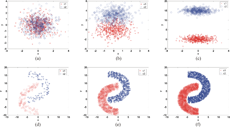
Figure 1: Examples of the artificial databases for clustering evaluation error. The first set points is generated according to a Gaussian distribution, where the two sets are separated by distances (a) $d=0$, (b) $d=3$ and (c) $d=15$. In the case of the second set, a higher density of points provides more defined clusters, as shown in examples (d) $\rho=1.0$, (e) $\rho=6.4$ and (f) $\rho=14.4$.

With respect to real-world databases, we take into account two datasets, i.e. the Iris database Fisher (1936), and the Breast Cancer Wisconsin database Wolberg et al. (1994). The Iris database is composed by three species of Iris flowers (Iris setosa, Iris virginica and Iris versicolor). Each class consists of 50 samples, where four features were measured from each sample, i.e. the length and the width of the sepal and the petal, in centimeters. On the other hand, the cancer database is composed by features of digitized image of a fine needle aspirate from a breast mass, where 30 real-valued features are computed for each cell nucleus Wolberg et al. (1994). This database is composed by 699 cells, where 241 are malignant and 458 are benign.

III Results and discussion

The accuracy of the clustering method based on networks is compared with four traditional clustering methods, namely k-means, cobweb, farthest first and expectation maximization (EM) Witten and Frank (2005). These methods present different properties, such as the k-means tendency to find spherical clusters Theodoridis and Koutroumbas (2003). Moreover, we consider three methods for community identification, namely fastgreedy, extremal optimization and walktrap Fortunato (2010). However, in this work, since the fastgreedy and extremal optimization result in the same error rates for all considered databases, we discuss only the results of the fastgreedy method, which is faster than the extremal optimization approach.

We start our analysis by taking into account the Iris and the Breast Cancer Wisconsin databases. As a preliminary data visualization, we project the patterns into a two dimensional space by taking into account principal component analysis. Figure 2 shows the projections. It is clear that there is no clear separation between the clusters for both databases.

Since the attributes in the Iris data present different ranges, having values such as 0.1 for the petal width and 7.2 for the sepal length, it is necessary to take into account a feature standardization procedure Theodoridis and Koutroumbas (2003). In this case, each attribute is transformed in order to present mean equals to zero and standard deviation equals to one. This transformation, called standardization, is performed as,

$$y_{f}=\frac{x_{f}-\overline{x_{f}}}{\sigma_{x_{f}}}$$ (12)

where $\overline{x_{f}}$, $\sigma_{x_{f}}$ are the average and standard deviation of the values of attribute $f$, respectively. The obtained results considering the four clustering algorithm is presented in Table 1. The EM and k-means exhibit the smaller errors among the traditional classifiers. However, note that this performance is obtained when the number of clusters is known. On the other hand, EM provides an error of 40% when the number of clusters is unknown. This is a limitation of these methods, since in most of the cases, the information about the number of classes is not available.

Table 1 also presents the results with respect to the cluster-based on complex networks approaches. Only combinations between metric and community algorithm which result in the smallest error rates are shown in this table. The smallest error was obtained by taking into account the inverse of the Chebyshev distance and the fastgreedy community identification algorithm. The obtained error for this case is equal to 4.7%. The second best performance is obtained by considering the inverse of the Euclidian distance and the fastgreedy or the walktrap algorithms, which provide an error of 6%. In addition to the smallest error rates, network-based clustering present other important feature, i.e. it is not necessary to specify the number of clusters present in the database. Indeed, the maximum value of the modularity suggests the most accurate partition. Nevertheless, for some proximity measures, the modularity is not able to determine the best partition. In this case, the knowledge about the number of clusters implies in a reduction of the error rates, as in the case of exponential of the Tanimoto distance, where the error is reduced from 33.3% to 6%, and the exponential of the Chebyshev distance, where the error is reduced from 33.3% to 7.3%. Therefore, for the Iris data, such metrics are not appropriated for network-based clustering. We also analyze the clustering error without standardization. In this case, the error rates are larger than those obtained considering the normalization, for some cases. However, for the best results, we verify that the errors are similar in both cases. Figure 3 presents the dendrogram obtained for the best separation, i.e. by taking into account the inverse of Chebyshev distance and the fastgreedy community identification method. Observe that the best partition is obtained for the highest value of the modularity measure.

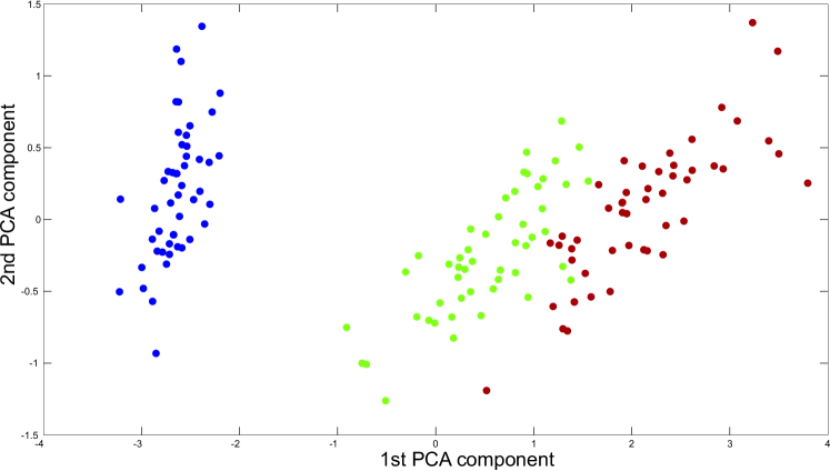
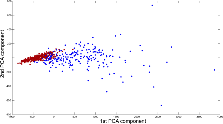
Figure 2: Projection of (a) the Iris and (b) the Breast Cancer Wisconsin databases by principal component analysis.

Table 1: Clustering errors for the Iris database considering the cases in which the number of classes $k$ is known ($k=3$) or unknown ($k=?$). EM and k-means are the only methods that need to specify the number of clusters $k$.

Method	% error ($k=?$)	% error ($k=3$)
k-means	–	11.3
cobweb	33.3	–
farthest first	–	14.0
EM	40.0	9.3
$D_{E}^{-1}$ - fastgreedy	6.0	6.0
$D_{E}^{-1}$ - walktrap	6.0	6.0
$S_{E}$ - walktrap	33.3	14.7
$S_{T}$ - walktrap	33.3	6.0
$S_{F}$ - walktrap	33.3	7.3
$D_{M}^{-1}$ - fastgreedy	33.3	6.0
$D_{M}^{-1}$ - walktrap	33.3	6.0
$S_{M}$ - walktrap	33.3	6.0
$D_{C}^{-1}$ - fastgreedy	4.7	4.7
$D_{C}^{-1}$ - walktrap	9.3	9.3
$S_{C}$ - Walktrap	33.3	7.3

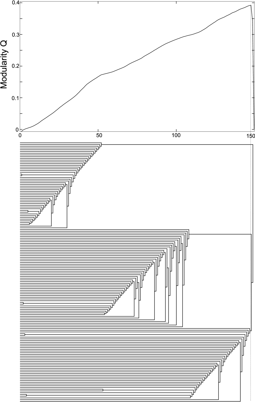
Figure 3: Dendrogram obtained by taking into account the inverse of Chebyshev distance and the fastgreedy community identification algorithm for the Iris data. The cut in the dendrogram results in three classes, where the error rate is equal to 4.7%.

The cancer database also needs to be pre-processed by the standardization. The obtained clustering errors are presented in Table 2. Only combinations between metric and community algorithm which result in the smallest error rates are shown in this table. In this case, the smallest clustering error is obtained by the k-means method, which produces an error rate of 7.2%. However, the complex networks-based method taking into account the inverse of Manhattan distance and walktrap algorithm for community identification provides an error rate of 7.9%. Observe that when the number of clusters is known, all methods result in smaller error rates. Nevertheless, the $D_{M}^{-1}$-walktrap produces the same error rate of 7.9% even when $k=2$. Therefore, the highest value of the modularity accounts for the separation for this method. Although our proposed method implied in an higher error than the k-means methodology, it presents the advantage that it is not necessary to known the number of clusters. In this way, our methodology is also more suitable to determine the clusters for the Breast Cancer Wisconsin database.

Table 2: Clustering errors for the Breast Cancer Wisconsin database considering the cases in which the number of classes $k$ is known ($k=3$) or unknown ($k=?$). EM and k-means are the only methods that need to specify the number of clusters $k$.

Method	% error (k=?)	% error (k = 3)
k-means	–	7.2
cobweb	37.2	–
farthest first	–	35.3
EM	75.9	8.8
$D_{E}^{-1}$ - walktrap	52.9	9.8
$S_{F}$ - fastgreedy	17.6	17.6
$D_{M}^{-1}$ - walktrap	7.9	7.9
$D_{C}^{-1}$ - fastgreedy	50.8	15.3
$S_{C}$ - walktrap	15.9	15.9

In order to provide a more comprehensive evaluation of the proposed complex networks-based clustering approach, we generated two set of artificial data into a two dimensional space, as discussed in the last section. This artificial data allows to control the cluster separability of the generated databases. Initially, we consider two clusters of points with Gaussian distribution in an two-dimensional space separated by a distance $d$. Figure 4 presents the best obtained results for the complex networks-based approach taking into account different proximity measures. For all cases, the number of clusters is determined automatically by the maximum value of the modularity. Note that the error rate goes to zero for $d\geq 5$. Figure 4(f) shows the comparison between the traditional clustering method which resulted in the best results, i.e. the cobweb, and the best complex networks approach. In this case, the method based on the exponential of the Chebyshev distance and fastgreedy algorithm provides the smallest error rate. Observe that the variation of the error rate is also small for this method, compared with the cobweb.

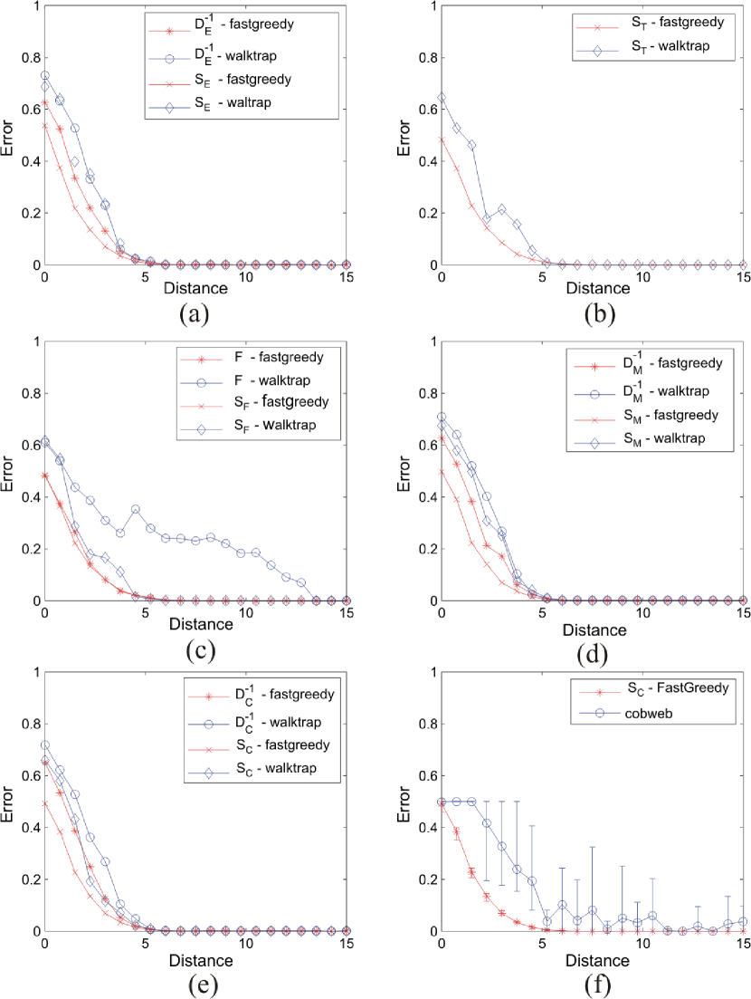
Figure 4: Error rates obtained according to the separation of two clusters composed by sets of points with gaussian distribution in a two-dimensional space. We show the best results for each proximity measure, i.e. (a) Euclidian, (b) Tanimoto, (c) Fu, (d) Manhattan and (e) Chebyshev distances. The number of clusters is determined automatically by the maximum value of the modularity for all cases. In (f) the most accurate network-based method is compared with the best traditional clustering approach. Each point is an average over 10 simulations.

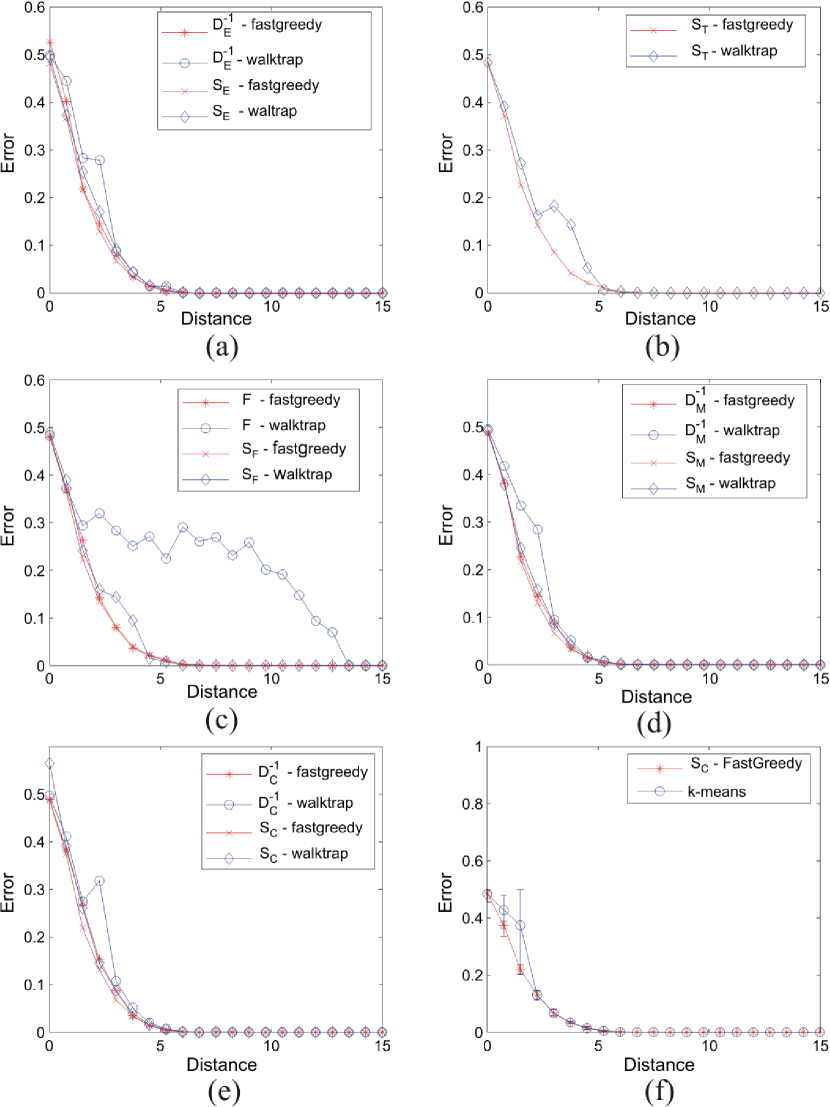
Figure 5: Error rates obtained according to the separation of two clusters composed by sets of points with Gaussian distribution in a two-dimensional space for the case where the number of clusters is known. We show the best results for each proximity measure, i.e. (a) Euclidian, (b) Tanimoto, (c) Fu, (d) Manhattan and (e) Chebyshev distances. The number of clusters is set as $k=2$ for all methods. In (f) it the most accurate network-based method is compared with the best traditional clustering approach. Each point is an average over 10 simulations.

The k-means algorithm cannot be used in the comparison where the number of clusters $k$ is known. Thus, we consider the case where $k$ is determined for all methods. Figure 5 presents the obtained results. In all cases, the error rate goes to zero for $d\geq 5$. As in the case of unknown number of clusters, the method based on the exponential of the Chebyshev distance and fastgreedy algorithm provides the smallest error rate. Among the traditional algorithms, the k-means allows the most accurate results. In fact, for $d\geq 3$, both k-means and network-based clustering method provide similar error rates. For this database, accurate results were expected for the k-means method, since the clusters are symmetric around the means, being equally distributed among the two clusters. Observe that the other approaches of the complex networks-based method also imply in an small error rate. Comparing with the cases where the number of clusters is unknown, i.e. Figure 4 shows that the error rate is similar for both approaches. Therefore, the network-based methods result in the most accurate cluster partitions and have the advantage that it is not necessary to know the number of clusters.

The second artificial database used to evaluate the classification error rates is given by the two semi-circle with varying density of points (see Figures 1(d) – (f)). Figure 6 presents the obtained results for unknown number of clusters considering fastgreedy algorithm. Only the best results are shown in this figure. The higher the density of points, the smaller the error rate, since the clusters become more defined. The error rate does not tend to zeros only for the inverse of the Chebyshed distance (Figure 6(c)). The most accurate clustering is obtained by taking into account the exponential of the Manhattan distance (Figure 6(b)). Figure 7 presents the obtained errors when the number of clusters is known, i.e. $k=2$. Again, the complex networks-based method which takes into account the exponential of the Manhattan distance produces the smallest error. It is interesting to note that the traditional clustering methods, i.e. k-means and cobweb, result in higher error rates than the methods based on complex networks. In addition, the error does not tend to zero when the density of points is increased for these traditional methods. Figure 8 presents an example of the best clustering for the k-means and complex networks-based methods. Observe that k-means cannot identify the correct clusters.

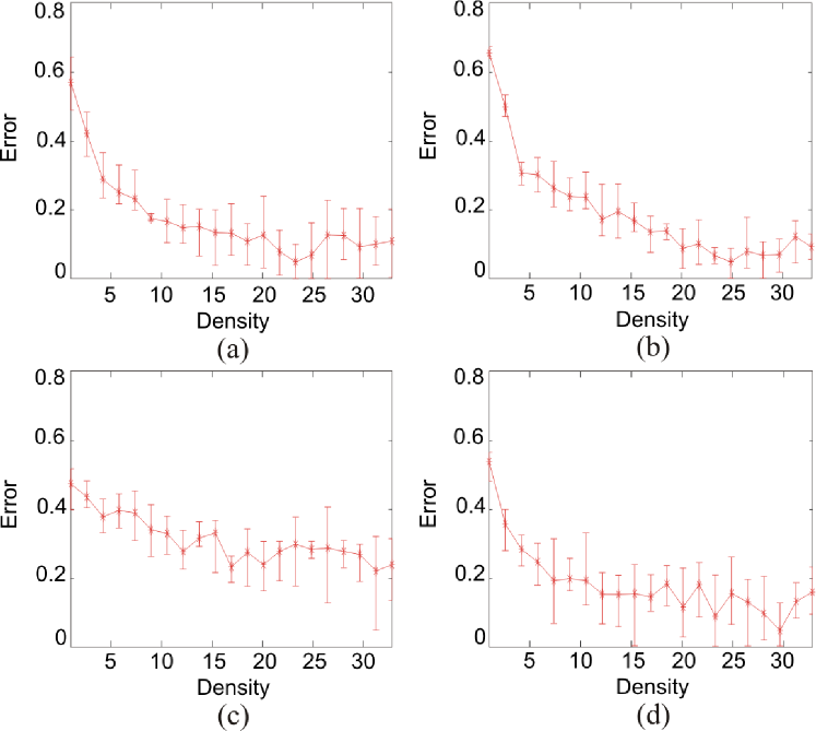
Figure 6: The smallest clustering errors obtained for the complex networks-based methods applied in the second artificial dataset (see Figures 1(d) – (f)). The error rates are determined according to the density of points. The adopted proximity measures are (a) the exponential of the Euclidian distance, (b) the exponential of the Manhattan distance, (c) the inverse of the Chebyshev distance and (d) the exponential of the Chebyshev distance. The number of clusters is obtained automatically by the maximum value of the modularity.

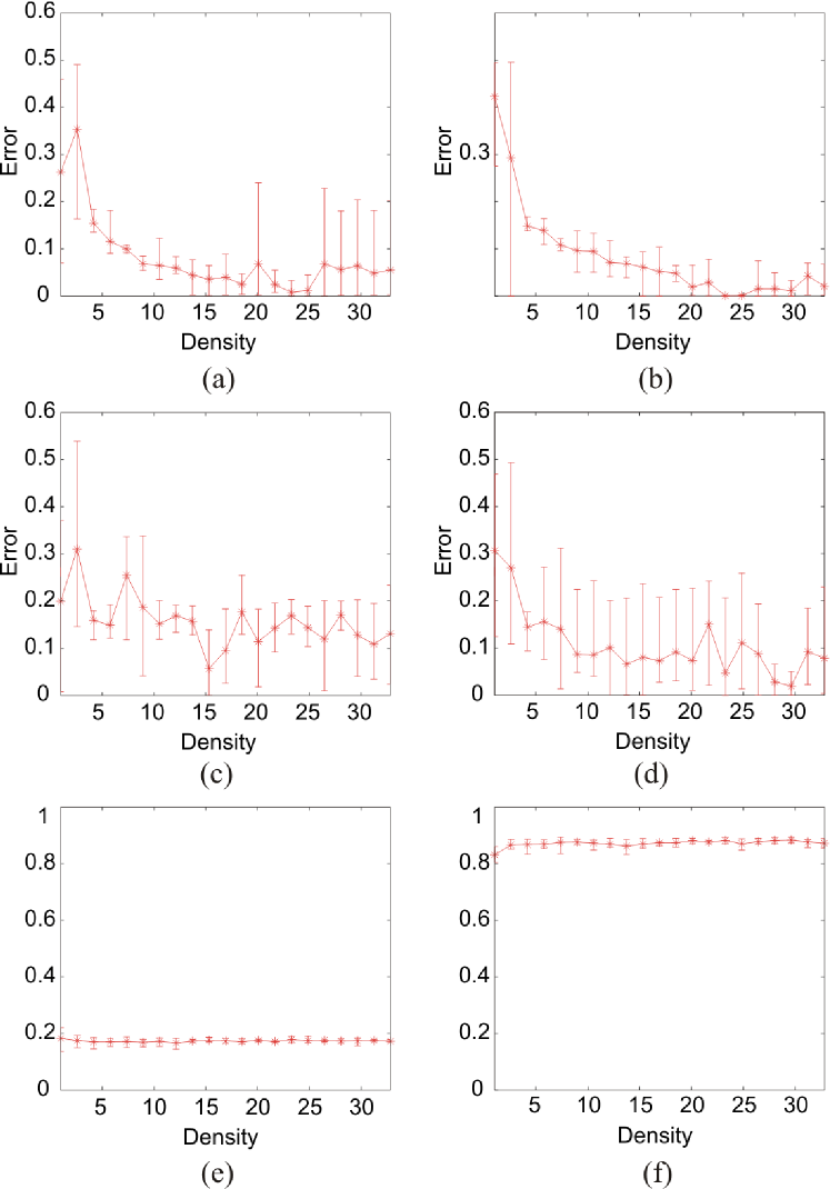
Figure 7: The smallest clustering errors obtained for the complex networks-based methods applied in the second artificial dataset (see Figures 1(d) – (f)). The error rates are determined according to the density of points. The adopted proximity measures are (a) the exponential of the Euclidian distance, (b) the exponential of the Manhattan distance, (c) the inverse of the Chebyshev distance and (d) the exponential of the Chebyshev distance. The number of clusters is fixed as $k=2$. The k-means (e) and cobweb (f) are the traditional clustering methods that produce the smallest errors.

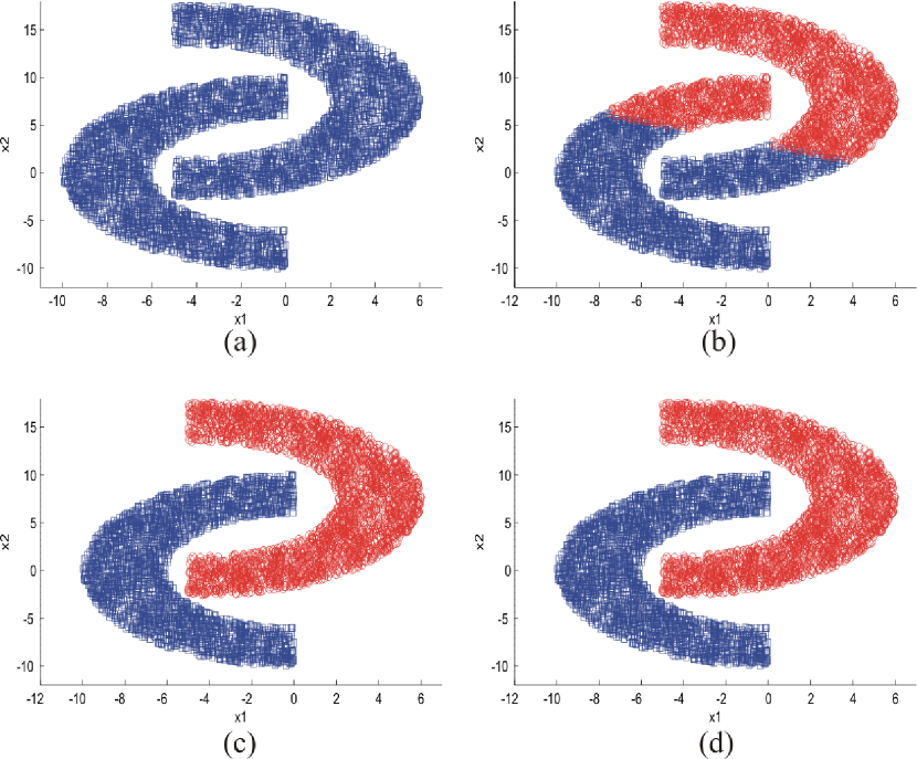
Figure 8: Example of the best performance for the (b) k-means, complex network-based methods method using (c) the best modularity value and (d) fixing $k=2$. The original data is shown in (a).

IV Conclusion

In this work, we study different proximity measures to represent a data set into a graph and then adopt community detection algorithms to perform respective clustering. Our obtained results suggest that complex networks theory has tools to improve graph-based clustering methodologies, since this new area provides more accurate algorithms for community identification. In fact, comparing with traditional clustering methods, the network-based approach finds clusters with the smallest error rates for both real-world and artificial databases. In addition, this methodology allows the identification of the number of clusters automatically by taking into account the maximum value of the modularity measurement. Among the considered proximity measures, the inverse of the Chebyshev distance and the inverse of the Manhattan distance are the most suitable metric for the considered real-world databases. With respect to the artificial databases, the exponential of the Chebyshev and exponential of the Manhattan distance produces the smallest error rates. Therefore, metrics based on the Chebyshed and Manhattan distances are the most suitable to quantify the similarity between objects in terms of their feature vectors. Among the community identification algorithms, the fastgreedy revealed to be the most suitable, due to its accuracy and the smallest time for processing.

The analysis proposed in this work can be extended by taking into account other real-world databases as well as other approaches to generate artificial clusters. The application to different areas, such as medicine, biology, physics and economy constitute other promising research possibilities.

References

- Anderberg (1973) M. Anderberg, Cluster Analysis for Applications (1973).
- Jain et al. (1999a) A. Jain, M. Murty, and P. Flynn, ACM Computing Surveys 31, 264 (1999a), ISSN 0360-0300.
- Everitt et al. (2001) B. S. Everitt, S. Landau, and M. Leese, Cluster analysis (Arnold, 2001).
- Theodoridis and Koutroumbas (2003) S. Theodoridis and K. Koutroumbas, Pattern recognition (Academic Press, 2003).
- Jain et al. (1999b) A. Jain, M. Murty, and P. Flynn, ACM computing surveys (CSUR) 31, 264 (1999b), ISSN 0360-0300.
- Zahn (2006) C. Zahn, Computers, IEEE Transactions on 100, 68 (2006), ISSN 0018-9340.
- Urquhart (1982) R. Urquhart, Pattern recognition 15, 173 (1982), ISSN 0031-3203.
- Koontz et al. (2006) W. Koontz, P. Narendra, and K. Fukunaga, Computers, IEEE Transactions on 100, 936 (2006), ISSN 0018-9340.
- Newman and Girvan (2004) M. Newman and M. Girvan, Physical review E 69, 26113 (2004), ISSN 1550-2376.
- de Oliveira et al. (2008) T. de Oliveira, L. Zhao, K. Faceli, and A. de Carvalho, in IEEE Congress on Evolutionary Computation, 2008. CEC 2008.(IEEE World Congress on Computational Intelligence) (2008), pp. 2121–2126.
- Karypis et al. (2002) G. Karypis, E. Han, and V. Kumar, IEEE Computer 32, 68 (2002), ISSN 0018-9162.
- Fortunato (2010) S. Fortunato, Physics Reports 486, 75 (2010), ISSN 0370-1573.
- Albert and Barabási (2002) R. Albert and A.-L. Barabási, Reviews of Modern Physics 74, 48 (2002).
- da F. Costa et al. (2007) L. da F. Costa, F. A. Rodrigues, G. Travieso, and P. R. V. Boas, Advances in Physics 56, 167 (2007).
- Newman (2010) M. E. J. Newman, Networks: An Introduction (Oxford Univ Pr, 2010), ISBN 0199206651.
- Bullmore and Sporns (2009) E. Bullmore and O. Sporns, Nature Reviews Neuroscience 10, 186 (2009), ISSN 1471-003X.
- Newman (2006) M. Newman, Proceedings of the National Academy of Sciences 103, 8577 (2006).
- Girvan and Newman (2002) M. Girvan and M. Newman, Proceedings of the National Academy of Sciences of the United States of America 99, 7821 (2002).
- Clauset et al. (2004) A. Clauset, M. E. J. Newman, and C. Moore, Physical Review E 70, 066111 (2004).
- Clauset (2005) A. Clauset, Physical Review E 72, 026132 (2005).
- Fisher (1936) R. A. Fisher, Annals Eugenics 7, 12 (1936).
- Duch and Arenas (2005) J. Duch and A. Arenas, Physical Review E 72, 027104 (2005).
- Pons and Latapy (2005) P. Pons and M. Latapy, Computer and Information Sciences-ISCIS 2005 pp. 284–293 (2005).
- Danon et al. (2005) L. Danon, J. Duch, A. Arenas, and A. Díaz-Guilera, Journal of Statistical Mechanics: Theory and Experiment p. P09008 (2005).
- Wolberg et al. (1994) W. Wolberg, W. Street, and O. Mangasarian, Cancer Letters 77, 163 (1994), ISSN 0304-3835.
- Witten and Frank (2005) I. Witten and E. Frank, Data Mining: Practical machine learning tools and techniques (Morgan Kaufmann Pub, 2005), ISBN 0120884070.