Hybrid Monte Carlo Simulation of Graphene on the Hexagonal Lattice

Abstract

We present a method for direct hybrid Monte Carlo simulation of graphene on the hexagonal lattice. We compare the results of the simulation with exact results for a unit hexagonal cell system, where the Hamiltonian can be solved analytically.

I Introduction

Graphene, a single layer of carbon atoms forming a hexagonal lattice, has remarkable properties graphene . In the tight-binding approximation the quadratic Hamiltonian gives origin to a dispersion formula which for low momenta is analogous to the dispersion formula for relativistic fermions in two dimensions dispersion . This has prompted some researchers to adapt to graphene lattice gauge theory techniques which have been profitably used for the study of Quantum Chromodynamics and other particle systems LGT . In the work of LGT-graphene one approximates first the tight-binding Hamiltonian of graphene with a Dirac Hamiltonian, incorporates the Coulomb interaction through the introduction of a suitable electromagnetic field, and finally discretizes the resulting continuum quantum field theory on a hypercubic space-time lattice. The hybrid Monte Carlo method HMC , widely used in lattice gauge theory to simulate fermions interacting with quantum gauge fields, can then be used to investigate the effects of the Coulomb interaction in the graphene system.

The approach outlined above has led to very interesting and valuable results LGT-graphene , yet one would think that, since the starting point is a system already defined on a lattice, it should be possible to apply the hybrid Monte Carlo technique directly to the graphene lattice. The clear advantage of this approach is the direct connection to the experimentally determined physical lattice constants of the tight-binding model, which represents an accurate description of the experimental system. In this letter we illustrate how this can be done.

Graphene is a system of interacting electrons located at the vertices of a hexagonal lattice. It is convenient to think of the graphene lattice as consisting of two triangular sublattices, which we denote by $A$ and $B$, which together with the centers of the hexagons (sublattice $C$) form a finer, underlying triangular lattice (Fig. 1). We introduce fermionic annihilation and creation operators $a_{x,s},a^{\dagger}_{x,s}$ for the electrons on the two sublattices, where $x$ is a site index and $s=\pm 1$ is the spin index. The lattice must be made finite in order to perform numerical simulations. While there is a broad range of boundary conditions of physical interest, here we consider periodic systems formed by identifying opposing sides of a hexagonal lattice of length $L$, illustrated in Fig. 1 for $L=4$.

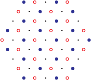
Figure 1: The hexagonal graphene lattice consists of the two triangular sublattices $A$ (solid) and $B$ (empty), which together with the centers of the hexagons (dots) form a finer, underlying triangular lattice.

The tight-binding Hamiltonian $H$ consists of two terms: the quadratic kinetic term,

$$H_{2}=\sum_{\langle x,y\rangle,s}-\kappa(a^{\dagger}_{x,s}a_{y,s}+\mbox{h.c.}),$$ (1)

where the sum runs over all pairs $\langle x,y\rangle$ of nearest neighbor sites (coupling the $A$ and $B$ sublattices) and the two values of the spin, and the Coulomb interaction Hamiltonian,

$$H_{C}=\sum_{x,y}e^{2}V_{x,y}q_{x}q_{y},$$ (2)

where

$$q_{x}=a^{\dagger}_{x,1}a_{x,1}+a^{\dagger}_{x,-1}a_{x,-1}-1$$ (3)

is a local charge operator and $V$ is the interaction potential. We have explicitly introduced the charge coupling constant $e$.

Several comments are in order. First note that in the kinetic term we have neglected the smaller next-to-nearest neighbor hopping within each sublattice, which would introduce a small (probably manageable) complex phase in the path integral. The charge operator Eq. 3 has a $-1$ to account for the background charge of the carbon ion: it ensures that the system is neutral at half filling, and it will play an important role for our functional integral formulation. $V$ could be the actual 3d Coulomb potential, but could be any other interaction potential. The only thing crucial for us is that the matrix $V_{x,y}$ be positive definite. Finally, we note that the Hamiltonian of Eqs. 1-2 commutes with the isospin generators

$$I_{\pm} =a^{\dagger}_{x,s}\sigma^{ss^{\prime}}_{\pm}a_{x,s^{\prime}}, I_{3} =a^{\dagger}_{x,s}\sigma^{ss^{\prime}}_{3}a_{x,s^{\prime}}/2.$$ (4)

In order to explore the properties of the system one would like to calculate expectation values,

$$\langle{\cal O}_{1}(t_{1}){\cal O}_{2}(t_{2})\dots\rangle=Z^{-1}\mbox{Tr}\,T[{\cal O}_{1}(t_{1}){\cal O}_{2}(t_{2})e^{-\beta H}]\;,$$ (5)

where $\beta$ can be interpreted as an extent in Euclidean time, $T[\dots]$ stands for time ordering of the operators inside the square bracket with respect to the Euclidean evolution implemented by $\exp(-\beta H)$, and $Z=\mbox{Tr}\,\exp(-\beta H)$ is the partition function.

II Path integral form

Our goal is to provide an equivalent path integral formulation of Eq. 5 conducive to calculation by numerical simulation, following a rather standard procedure to convert from the Hamiltonian into a Lagrangian. We will first express the expectation values and the partition function in terms of an integral over anticommuting fermionic fields, i.e. elements of a Grassmann algebra. (The literature on the path integral formulation of quantum expectation values is very rich. In our work we followed the very clear and useful formulation given in the first chapters of Negele-Orland .) This gives origin to an integrand with an exponential containing a quadratic form in the fermionic fields, from $H_{2}$ and the normal ordering of $H_{C}$, as well as a quartic expression, from $H_{C}$. The quartic expression can be reduced to a quadratic form by a Hubbard-Stratonovich transformation HST , through the introduction of a suitable auxiliary bosonic field (in our case a real field), and now the Gaussian integral over the elements of the fermionic variables can be explicitly performed, leaving an integral over the bosonic field only. The problem, however, is to obtain an integral that can be interpreted as an integration over a well defined probabilistic measure, which can thus be approximated by stochastic simulation techniques. We will show here how the symmetries of the system make this possible.

We start by rewriting the expression for the charge as

$$q_{x}=a^{\dagger}_{x,1}a_{x,1}-a_{x,-1}a^{\dagger}_{x,-1}.$$ (6)

We now introduce hole creation and annihilation operators for the electrons with spin $-1$:

$$b^{\dagger}_{x}=a_{x,-1},\quad b_{x}=a^{\dagger}_{x,-1}$$ (7)

so that the charge becomes

$$q_{x}=a^{\dagger}_{x}a_{x}-b^{\dagger}_{x}b_{x}.$$ (8)

Note that we dropped the spin indices since from now on $a,a^{\dagger}$ and $b,b^{\dagger}$ will always refer to spin 1 and $-1$, respectively. Finally we change the sign of the $b,b^{\dagger}$ operators on one of the sublattices. The crucial constraint is that all redefinitions of the operators respect the anticommutator algebra. From the fact that $H_{2}$ only couples sites on the two different sublattices, it follows that $H_{2}$ now takes the form

$$H_{2}=\sum_{\langle x,y\rangle}-\kappa(a^{\dagger}_{x}a_{y}+b^{\dagger}_{x}b_{y}+\mbox{h.c.}).$$ (9)

We introduce fermionic coherent states

$$|\psi,\eta\rangle = e^{-\sum_{x}(\psi_{x}a^{\dagger}_{x}+\eta_{x}b^{\dagger}_{x})}|0\rangle,$$

$$\langle\psi^{*},\eta^{*}| = \langle 0|e^{-\sum_{x}(a_{x}\psi_{x}+b_{x}\eta_{x})}$$ (10)

where $\psi_{x},\psi_{x}^{*},\eta_{x},\eta_{x}^{*}$ are anticommuting fermionic variables (elements of a Grassmann algebra).

The path integral formulation is obtained by factoring

$$e^{-\beta H}=e^{-H\,\delta}e^{-H\,\delta}\dots e^{-H\,\delta}\quad(N_{t}\;\mbox{terms})$$ (11)

with $\delta=\beta/N_{t}$, and then inserting repeatedly among the factors the resolution of the identity expressed in terms of an integral over the fermionic variables. The trace in Eq. 5 must also be expressed in terms of a similar integral. (See e.g. Negele-Orland for details.) This leads to integrals over fermionic fields $\psi_{x,t},\psi_{x,t}^{*},\eta_{x,t},\eta_{x,t}^{*}$ (the index $t=0,N_{t}-1$ appears because of the multiple resolutions of the identity and can be thought of as an index labeling Euclidean time), which contain in the integrand expressions of the type

$$\langle\psi^{*}_{x,t},\eta^{*}_{x,t}|e^{-H\,\delta}|\psi_{x,t},\eta_{x,t}\rangle.$$ (12)

The last ingredient is the identity

$$\begin{split}&\langle\psi^{*}_{x,t},\eta^{*}_{x,t}|F(a_{x}^{\dagger},b_{x}^{\dagger},a_{x},b_{x})|\psi_{x,t},\eta_{x,t}\rangle\\ &\quad=F(\psi_{x,t}^{*},\eta_{x,t}^{*},\psi_{x,t},\eta_{x,t})e^{\sum_{x}(\psi^{*}_{x,t}\psi_{x,t}+\eta^{*}_{x,t}\eta_{x,t})}\end{split}$$ (13)

which is true of any normal ordered function $F$ of the operators $a_{x}^{\dagger},b_{x}^{\dagger},a_{x},b_{x}$.

The Hamiltonian is in fact already in normal order except for the local term $e^{2}V_{xx}q_{x}q_{x}$, which can be written as the sum of two normal-ordered pieces,

$$e^{2}V_{xx}q_{x}q_{x}=e^{2}V_{xx}:q_{x}q_{x}:+\;e^{2}V_{xx}(a^{\dagger}_{x}a_{x}+b^{\dagger}_{x}b_{x}).$$ (14)

By reassigning the quadratic term in Eq. 14 to $H_{2}$, the exponent $-H\,\delta$ in Eq. 12 is normal ordered but the exponential $\exp(-H\,\delta)$ is not. However $\exp(-H\,\delta)$ differs from its normal ordered form $:\exp(-H\,\delta):$ by terms $O(\delta^{2})$. So, in the limit of $N_{t}\to\infty$ one may replace the operator expression $\exp(-H\,\delta)$ with an exponential involving the fermionic fields, as follows from Eq. 13. This leads to the following expression for the partition function

$$Z =\lim_{N_{t}\to\infty}\int\prod_{m=0}^{N_{t}-1}d\psi_{m}^{*}d\psi_{m}d\eta_{m}^{*}d\eta_{m}$$ (15)

$$\!\times e^{-\sum_{m,n}(\psi^{*}_{m}M_{m,n}\psi_{n}+\eta^{*}_{m}M_{m,n}\eta_{n})}e^{-\sum_{x,y,t}e^{2}Q_{x,t}V_{x,y}Q_{y,t}\delta}$$

where $Q_{x,t}=\psi^{*}_{x,t}\psi_{x,t}-\eta^{*}_{x,t}\eta_{x,t}$ and we have used $m$ (or $n$) as a shorthand for the indices $x,t$. $M$ is a matrix whose components may be deduced from

$$\sum_{m,n} \psi^{*}_{m}M_{m,n}\psi_{n}=\sum_{t}\Big{[}\sum_{x}\psi^{*}_{x,t}(\psi_{x,t+1}-\psi_{x,t})$$ (16)

$$+e^{2}V_{xx}\psi^{*}_{x,t}\psi_{x,t}-\kappa\sum_{\langle x,y\rangle}(\psi^{*}_{x,t}\psi_{y,t}+\psi^{*}_{y,t}\psi_{x,t})\,\delta\Big{]}$$

where $\psi_{x,N_{t}}$ must be identified with $-\psi_{x,0}$.

We now perform a Hubbard-Stratonovich transformation, introducing c-number real variables $\phi_{x,t}$ to recast the exponential with the quartic term in the form

$$\begin{split}&e^{-\sum_{x,y,t}e^{2}Q_{x,t}V_{x,y}Q_{y,t}\delta}=\int\prod_{x,t}d\phi_{x,t}\\ &\quad\times e^{-\sum_{x,y,t}\phi_{x,t}(V^{-1})_{x,y}\phi_{y,t}\delta/4}e^{-\sum_{x,t}\imath e\phi_{x,t}Q_{x,t}\delta},\end{split}$$ (17)

where we have absorbed a constant measure factor in the definition of the integral over $\phi_{x,t}$.

Inserting the r.h.s. of Eq. 17 into Eq. 15 we get

$$Z= \lim_{N_{t}\to\infty}\int\prod_{x,t}d\psi_{x,t}^{*}d\psi_{x,t}d\eta_{x,t}^{*}d\eta_{x,t}d\phi_{x,t}$$

$$\times e^{-\sum_{x,y,t}\phi_{x,t}(V^{-1})_{x,y}\phi_{y,t}\delta/4}$$

$$\times e^{-\sum_{x,t,y,\tau}(\psi^{*}_{x,t}M_{x,t;,y,\tau}\psi_{y,\tau}+\eta^{*}_{x,t}M_{x,t;y,\tau}\eta_{y,\tau})}$$

$$\times e^{-\sum_{x,t}\imath e\phi_{x,t}(\psi^{*}_{x,t}\psi_{x,t}-\eta^{*}_{x,t}\eta_{x,t})\delta}.$$ (18)

It is convenient to introduce a matrix $\Phi$ which is diagonal, with diagonal entries

$$\Phi_{x,t}=\phi_{x,t}\delta.$$ (19)

With this, Eq. 18 can be written in very compact form

$$\begin{split}Z=\int&d\phi d\psi^{*}d\psi d\eta^{*}d\eta\\ &\times e^{-\phi V^{-1}\phi\delta/4-\psi^{*}(M+\imath e\Phi)\psi-\eta^{*}(M-\imath e\Phi)\eta}\end{split}$$ (20)

where we have used matrix notation for all the sums and have dropped the limit notation.

The Gaussian integration over the anticommuting variables can now be done to obtain

$$Z=\int d\phi e^{-\phi V^{-1}\phi\delta/4}{\rm det}(M-\imath e\Phi){\rm det}(M+\imath e\Phi).$$ (21)

Because of the identity,

$$\det(M-\imath e\Phi)\det(M+\imath e\Phi)=\det[(M+\imath e\Phi)^{\dagger}(M+\imath e\Phi)]$$

the measure is positive definite. The down spins are treated as antiparticles (holes) moving backward in time relative to the up spins, exactly canceling the phase for each separately. Correlators for the fermion operators are now be obtained by integrating the appropriate matrix elements of $(M+\imath e\Phi)^{-1}$ or $(M-\imath e\Phi)^{-1}$ with the measure given by Eq. 21.

Equation 21 is the main result of our work. It establishes the partition function and expectation values as integrals over real variables with a positive definite measure. This is a crucial step for the application of stochastic approximation methods. There remains the problem of sampling the field $\phi_{x,t}$ with a measure which contains the determinant of a large matrix. But, following what is done in lattice gauge theory, this challenge can be overcome through the application of the hybrid Monte Carlo (HMC) technique HMC . In a broad outline, in HMC one first replaces the determinants in Eq. 21 with a Gaussian integral over complex pseudofermionic variables $\zeta_{x,t}$:

$$\begin{split}\det&\big{[}(M+\imath e\Phi)^{\dagger}(M+\imath e\Phi)\big{]}\\ &=\int d\zeta^{*}d\zeta e^{-\zeta^{*}(M+\imath e\Phi)^{{\dagger}\,-1}(M+\imath e\Phi)^{-1}\zeta}.\end{split}$$ (22)

(In this equation and in the following Eq. 23 we absorb an irrelevant, constant measure factor in the definition of the integrals.) One then introduces real “momentum variables” $\pi_{x,t}$ conjugate to $\phi_{x,t}$ and inserts in Eq. 22 unity written as a Gaussian integral over $\pi$. One finally arrives at

$$\begin{split}Z=&\int d\phi d\pi d\zeta^{*}d\zeta\\ &\times e^{-\phi V^{-1}\phi\delta/4-\zeta^{*}(M+\imath e\Phi)^{{\dagger}\,-1}(M+\imath e\Phi)^{-1}\zeta-\pi^{2}/2}.\end{split}$$ (23)

The idea of HMC is to consider the simultaneous distribution of the variables $\phi,\pi,\zeta$ and $\zeta^{*}$ determined by the measure in Eq. 23. The phase space of these variables is explored by first extracting the $\pi$, $\zeta$ and $\zeta^{*}$ according to their Gaussian measure, and then evolving the $\phi$ and $\pi$ variables with fixed $\zeta,\zeta^{*}$ according to the evolution determined by the Hamiltonian

$${\cal H}(\pi,\phi)=\frac{\pi^{2}}{2}+\frac{\phi V^{-1}\phi\delta}{4}+\zeta^{*}(M+\imath e\Phi)^{{\dagger}\,-1}(M+\imath e\Phi)^{-1}\zeta.$$ (24)

Because of Liouville’s theorem, the combined motion through phase space will produce an ensemble of variables distributed according to the measure in Eq. 23 and, in particular, of fields $\phi$ distributed according to the measure of Eq. 21.

Of course, the discussion above assumes that the Hamiltonian evolution of $\phi$ and $\pi$ is exact, which will not be the case with a numerical evolution. The HMC algorithm addresses this shortcoming by: 1) approximating the evolution with a symplectic integrator which is reversible and preserves phase space, 2) performing a Metropolis accept-reject step at the end of the evolution, based on the variation of the value of the Hamiltonian.

III Numerical Tests

We tested our method on the two-site system obtained by taking $L=1$, which can be solved exactly. We label the sites $x=0,1$. With $\kappa=1/3$, the Hamiltonian $H=H_{2}+H_{C}$ is now

$$H_{2} =-(a_{1}^{\dagger}a_{0}+a_{0}^{\dagger}a_{1}+b_{1}^{\dagger}b_{0}+b_{0}^{\dagger}b_{1})$$

$$\quad+\mu(a^{\dagger}_{0}a_{0}+b^{\dagger}_{0}b_{0}+a^{\dagger}_{1}a_{1}+b^{\dagger}_{1}b_{1})$$ (25)

$$H_{C} =2e^{2}(a_{0}^{\dagger}a_{0}-b_{0}^{\dagger}b_{0})(a_{1}^{\dagger}a_{1}-b_{1}^{\dagger}b_{1})+\frac{2e^{2}}{r_{0}}a_{0}^{\dagger}b_{0}^{\dagger}a_{0}b_{0}\;,$$

where we have taken $V_{0,1}=V_{1,0}=1/3$ and a local interaction term $V_{0,0}=V_{1,1}=1/r_{0}$. The radius $r_{0}$ sets the physical scale in lattice units for localization of the net charge at the carbon atom. It must be restricted to $r_{0}<1$ for stability of the vacuum. Also the normal ordering prescription for $e^{2}V_{xx}q_{x}q_{x}$ in Eq. 14 adds a new contribution to $H_{2}$ in the form of an $I_{3}$ “chemical potential” $\mu a^{\dagger}_{x,s}\sigma^{ss^{\prime}}_{3}a_{x,s^{\prime}}$. It is well known iso that an $I_{3}$ chemical potential for any value of $\mu$ does not introduce a phase in the measure. To maintain the full $SU(2)$ “flavor” symmetry of the tight-binding graphene Hamiltonian, we must set $\mu=e^{2}/r_{0}$. For the two-site system, the isospin generators of Eq. 4 become

$$I_{+}=I^{\dagger}_{-}=(-1)^{x}a^{\dagger}_{x}b^{\dagger}_{x}\mbox{ and }I_{3}=[a^{\dagger}_{x}a_{x}+b^{\dagger}_{x}b_{x}]/2-1,$$

allowing us to unambiguously classify the 16 states as degenerate $I=0,1/2,1$ isomultiplets: 5 singlets, 4 doublets and one triplet.

We compared HMC results for expectation values of several products of fermionic operators with the corresponding exact values, finding satisfactory agreement. For example, the correlation function

$$C_{a}(t)=\langle(a_{0}-a_{1})(t)\,(a_{0}^{{\dagger}}-a_{1}^{{\dagger}})(0)\rangle/2$$ (26)

is illustrated in Fig. 2, which shows HMC results converging to the exact correlators for both the free theory with $e=0$ and an interacting case with $e=0.5$.

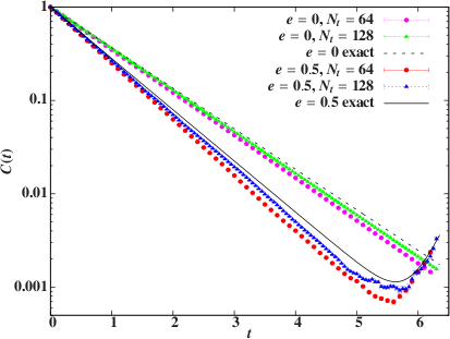
Figure 2: HMC data with $N_{t}=64$ and 128 converging to exact results for the correlation function of Eq. 26 with $\mu=e^{2}/r_{0}$, $r_{0}=1/2$ and fixed $\beta=N_{t}\delta=6.4$. The upper set of results are for $e=0$, the lower set for $e=0.5$.

A stringent test is to demonstrate the convergence to exact $SU(2)$ symmetry in the “time” continuum limit. To this end, consider a second correlation function,

$$C_{b}(t)=\langle(b_{0}^{{\dagger}}+b_{1}^{{\dagger}})(t)\,(b_{0}+b_{1})(0)\rangle/2\;,$$ (27)

related to $C_{a}(t)$ by an $SU(2)$ rotation. In Fig. 3 we compare HMC and exact results for both $C_{a}(t)$ and $C_{b}(t)$, finding that both correlators converge to the same continuum result.

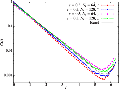
Figure 3: HMC data with $N_{t}=64$ and $N_{t}=128$ for the correlation functions of Eqs. 26 (“$\uparrow$”, red squares and blue triangles) and 27 (“$\downarrow$”, pink squares and green triangles) converging to the same exact continuum result (black solid line). Simulation parameters are the same as in Fig. 2.

We extract the energies of the isodoublet states at nonzero $\delta=\beta/N_{t}$ by fitting the correlator data in Fig 3 to single exponentials, $C(t)\approx e^{-Et}$ for fit range $0.4<t<4$. The results in Fig. 4 clearly show linear behavior $E\approx E_{0}+c_{1}\delta$, converging to the exact continuum energy is $E_{0}=e^{2}+\sqrt{4+e^{4}}-1\approx 1.266$. The continuum limit is consistent with restoration of the $SU(2)$ symmetry of the Hamiltonian: a simultaneous linear fit to both sets of energies gives $\lim_{\delta\to 0}E=1.262\pm 0.004$, with $c_{1}=1.25\pm 0.07$ and $-0.98\pm 0.04$ for correlators $C_{a}$ and $C_{b}$, respectively.

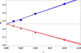
Figure 4: Linear extrapolation (including error band) of the HMC energies for isodoublet correlators $C_{a}(t)$ (blue dots) and $C_{b}$ (red triangles) as a function of the “time” lattice spacing $\delta=6.4/N_{t}$ for $N_{t}=32$, $64$, $128$ and $256$. The dotted horizontal line marks the exact continuum result.

IV Conclusion

While the results we reported are for a small test system, they demonstrate that HMC simulations of graphene directly on the hexagonal graphene lattice are possible and have the potential to produce valuable results. The dominant nearest neighbor hopping term has no sign problem, and we anticipate that a small next-to-nearest neighbor coupling $\kappa^{\prime}/\kappa\simeq 0.05$ can be accommodated by reweighting without a prohibitive cost. The crucial observation is the cancellation between the phase of the up spin and down spin determinant, when the latter are treated as holes moving backward in time. We are currently pursuing simulations of larger systems, and beginning to explore the many possible investigations and generalizations (e.g., distortions of the lattice, phonons, inclusion of magnetic fields).

Acknowledgments: We wish to acknowledge the many fruitful conversations with Dr. Ronald Babich, Prof. Antonio Castro Neto and Prof. Claudio Chamon during the course of this research and support under DOE grants DE-FG02-91ER40676, DE-FC02-06ER41440, and NSF grants OCI-0749317, OCI-0749202. Part of this work was completed while two of the authors were at the Aspen Center for Physics.

References

• (1) K. S. Novoselov et al., Science 306, 666 (2004).
• (2) A. H. Castro Neto et al., Rev. Mod. Phys. 81, 109 (2009).
• (3) H. J. Rothe, Lattice Gauge Theories: An Introduction, (World Scientific, Singapore, 2005).
• (4) J. E. Drut and T. A. Lähde, Phys. Rev. Lett. 102, 026802 (2009); Phys. Rev. B 79, 165425 (2009).
• (5) Simon Duane et al., Phys. Lett. B 195, 216 (1987).
• (6) J. W. Negele and H. Orland, Quantum Many Particle Systems, (Addison-Wesley, Redwood City, California, 1988).
• (7) R. L. Stratonovich, Sov. Phys. Dokl. 2, 416 (1958); J. Hubbard, Phys. Rev. Lett. 3, 77 (1959).
• (8) M. G. Alford, A. Kapustin and F. Wilczek, Phys. Rev. D 59, 054502 (1999); D. T. Son and M. A. Stephanov, Phys. Rev. Lett. 86, 592 (2001).