Unravelling the origins of S0 galaxies using maximum likelihood analysis of planetary nebulae kinematics

Abstract

To investigate the origins of S0 galaxies, we present a new method of analyzing their stellar kinematics from discrete tracers such as planetary nebulae. This method involves binning the data in the radial direction so as to extract the most general possible non-parametric kinematic profiles, and using a maximum likelihood fit within each bin in order to make full use of the information in the discrete kinematic tracers. Both disk and spheroid kinematic components are fitted, with a two-dimensional decomposition of imaging data used to attribute to each tracer a probability of membership in the separate components. Likelihood clipping also allows us to identify objects whose properties are not consistent with the adopted model, rendering the technique robust against contaminants and able to identify additional kinematic features.

The method is first tested on an N-body simulated galaxy to assess possible sources of systematic error associated with the structural and kinematic decomposition, which are found to be small. It is then applied to the S0 system NGC 1023, for which a planetary nebula catalogue has already been released and analyzed by Noordermeer et al., (2008). The correct inclusion of the spheroidal component allows us to show that, contrary to previous claims, the stellar kinematics of this galaxy are indistinguishable from those of a normal spiral galaxy, indicating that it may have evolved directly from such a system via gas stripping or secular evolution. The method also successfully identifies a population of outliers whose kinematics are different from those of the main galaxy; these objects can be identified with a stellar stream associated with the companion galaxy NGC 1023A.

1 Introduction

Lenticular or S0 galaxies lie between ellipticals and spirals on the Hubble sequence, since they have the featureless old stellar populations of elliptical systems, but also contain the disk components associated with spirals. They thus potentially represent a key element in attempts to understand the relationship between the main types of galaxy, but at the moment there is no consensus as to the end of the Hubble sequence to which they are most closely related. Clearly, some process has consumed their gas and shut off their star formation. However, this termination could be the result of galaxy mergers, much in the manner that star formation is believed to be quenched in elliptical galaxies, or it could arise from some much gentler process, such as ram pressure stripping, which simply removes the gas from normal spiral galaxies.

Perhaps the best way of discriminating between these scenarios is offered by the stellar dynamics of S0 galaxy disks. If they are the product of relatively gentle gas-stripping processes, one would expect the stellar dynamics to be unaffected, and should be identical to those of the progenitor spiral system, with rotation dominating relatively modest amounts of random motion in the disk (Aragón-Salamanca,, 2008; Williams et al., 2010). If, however, the S0s are the product of minor mergers, with a mass ratio higher than 10:1, one would expect the merging process to be imprinted in the stellar dynamics, with random velocities as high or even higher than the rotational velocities at all radii (Bournaud et al.,, 2005).

One difficulty in using such a diagnostic is that it requires accurate stellar kinematics measured in the outer parts of the galaxy where the disk dominates, and at low surface brightness, making conventional absorption-line spectroscopy difficult. However, planetary nebulae (PNe) provide an excellent probe of stellar kinematics in this regime: they are easily detected and can have their velocities measured from their characteristic strong emission lines, and they have proved to be an unbiased tracer of the global stellar population (Ciardullo et al.,, 1989, 2002; Napolitano et al., 2001; Coccato et al., 2009). We have designed and built a special-purpose instrument, the Planetary Nebula Spectrograph [PN.S; Douglas et al., (2002)], specifically to exploit this tracer of stellar kinematics at low surface brightnesses. Although originally intended to study elliptical galaxies (Romanowsky et al., 2003; Coccato et al., 2009; Napolitano et al., 2009), PN.S has already proved very effective in exploring the disks of spiral galaxies (Merrett et al., 2006), so an obvious next step was to use it to probe the kinematics of S0 systems.

As a pilot study, we observed the relatively nearby S0 galaxy NGC 1023 with PN.S. The observations and the resulting catalogue of positions and line-of-sight velocities of PNe are described in Noordermeer et al., (2008). The analysis in that paper concluded that NGC 1023 has very peculiar kinematics, giving the appearance of a normal rotationally-supported disk galaxy at small radii, but having entirely random velocities at large radii, inconsistent with either of the expected scenarios. However, the relatively simple dynamical analysis that led to these conclusions had some significant shortcomings. First, it assumed that the light at large radii was dominated by the disk component, and neglected any contribution from the spheroid. As we will see, this assumption can lead to sizable systematic errors in the inferred disk kinematics. Second, it calculated dynamical quantities such as velocity dispersions by binning the data both azimuthally and radially in the galaxy. Although such binning provides an adequate signal from a sparsely-sampled velocity field and a non-parametric measure of the local kinematics, as we will show below the kinematic properties vary continuously and quite rapidly with azimuth, so such binning averages away significant amount of information that is present in the raw data. The binning process also makes it difficult to identify any contamination from PNe that are either unrelated background objects, or lie within the system but do not match the expected kinematics.

In this paper, we therefore present a somewhat more sophisticated analysis designed to circumvent these shortcomings. While still binning the data in the radial direction, so as to extract a general non-parametric view of the galaxy’s dynamics, we apply a maximum likelihood analysis within each radial bin, so as to extract the maximum amount of information from the azimuthal variations in kinematic properties. We also model both disk and spheroid in the system, and use a full two-dimensional photometric decomposition of the galaxy, which allows us to allocate to each PN a probability as to the component to which it belongs.

The method we have developed to construct such a model is described in Section 2, and in Section 3 we test the technique on a simulated galaxy for which we have prior knowledge of the structural components and kinematics. In Section 4 we make a first real application of the method to the NGC 1023 catalogue, in which we show that this likelihood fitting can reproduce the strange results in Noordermeer et al., (2008) if we also neglect the spheroidal component, but that the more complete model presented here results in a picture in which NGC 1023 has a normal rotationally-supported disk. We also illustrate the power of likelihood fitting by showing how outlier points can be identified in the catalogue, and associated with a minor on-going merger. The conclusions are presented in Section 5.

2 Kinematic Likelihood Fitting

In this section we give a brief introduction to likelihood analysis, before going on to the specifics of fitting particular galaxy models. In Section 2.1, we present the case of a pure disk galaxy, as it provides both a simple example of the technique and a useful point of comparison to previous analyses that have assumed that the disk is the dominant component. In Section 2.2, we proceed to the more realistic situation in which we model both disk and spheroidal component. In Section 2.3 we discuss how the individual discrete kinematic tracers can be assigned, at least in a probabilistic sense, to either the disk or the spheroid using photometric data.

In general, given a set of $N$ independent velocity measurements, $v_{i}=(v_{1},...,v_{N})$, drawn from a probability density function $F(v_{i};\vec{\theta})$, where $\vec{\theta}=(V,\sigma)$ is a set of parameters whose value is unknown, the likelihood function is given by

$$\mathcal{L}=\prod_{i}F(v_{i};\vec{\theta}).$$ (1)

The values of ${V}$ and ${\sigma}$ that maximize $\mathcal{L}$ are the best estimators for the true values of these parameters. Moreover the method of maximum likelihood coincides with the method of the least squares in the special case of a set of $N$ Gaussian distributed independent measurements, in which case the likelihood function is directly related to the usual $\chi^{2}$ statistic,

$$\Delta\chi^{2}(\vec{\theta})=-2\Delta\ln\mathcal{L}(\vec{\theta}).$$ (2)

Thus, in this case it is straightforward to determine the confidence region around the best estimator:

$$\ln\mathcal{L}(\vec{\theta})\geq\ln\mathcal{L}_{max}-\Delta\ln\mathcal{L},$$ (3)

where values of $\Delta\chi^{2}$ or $-2\Delta\ln\mathcal{L}$, corresponding to a desired confidence limit, for joint estimation of $m$ parameters, are readily available in tabulated form. In this paper we use a $\Delta\chi^{2}$ that corresponds to a $1\sigma$ coverage probability. In particular, $\Delta\chi^{2}=5.39$ for $m=4$, and $\Delta\chi^{2}=4.11$, for $m=3$.

Finally, once the best-fit parameters have been found, one can calculate the contribution of each data point to the likelihood given this optimum model. To quantify this contribution in terms of whether the kinematic tracer in question is consistent with being drawn from the best-fit model, one can generate a large number of individual velocities drawn from a velocity distribution matching the model, and see at what percentile of the distribution the data point lies. We can thus identify any objects whose velocities lie outside this confidence interval, which are most likely interlopers. By rejecting these data points and iterating on the fit, we can render this process robust against a small amount of contamination, in a straightforward generalization of the $3\sigma$ clipping procedure (Merrett et al., 2003) used in determining membership of velocity distributions that are assumed to be Gaussian. We define the likelihood clipping probability threshold as the value at which we cut the distribution, and we reject all the PNe beyond this limit.

In principle, such likelihood fitting could be applied to a full dynamical model across an entire galaxy, at all radii and azimuths. However, in this analysis we are interested in leaving as much freedom as possible in the resulting radial profile of dynamical properties, so as to explore the full range of possibilities predicted by different models of S0 formation. We therefore adopt a hybrid approach in which the data are binned into elliptical annuli matched to the inclination of the disk, to extract points over a range of intrinsic radii. This binning allows each section of the disk to be modeled as an independent non-parametric data point. However in the azimuthal direction around each bin we use a full likelihood analysis that accurately models the expected variation in the line-of-sight velocity distribution with azimuth, as derived from very general dynamical considerations.

2.1 Likelihood analysis for a disk model

Consider a general rotating disk model for a galaxy. Part of the line-of-sight velocity of each object within it, $v_{i}$, is the projection of the galaxy’s mean rotation velocity $V$, at an azimuthal angle $\phi$ within the galaxy, corrected for the inclination of the galaxy to the line of sight $i$, and for the systemic velocity of the galaxy itself $V_{sys}$:

$$V_{los}=V_{sys}+V\sin(i)\cos(\phi).$$ (4)

Superimposed on the net rotational velocity are the random motions of the individual stars, which can be quantified by their velocity dispersion in different directions. For an axisymmetric disk, these components are most naturally expressed in cylindrical polar coordinates aligned with the axis of symmetry, ($R,\phi,z$), and the line-of-sight velocity dispersion, $\sigma_{los}$, is made up from a projection of these components such that

$$\sigma^{2}_{los}=\sigma^{2}_{r}\sin^{2}i\sin^{2}\phi+\sigma^{2}_{\phi}\sin^{2}i\cos^{2}\phi+\sigma^{2}_{z}\cos^{2}i$$ (5)

Generally speaking, in disk galaxies, $\sigma_{z}$ is the smallest component of the velocity dispersion, and in a nearly edge-on galaxy, like the ones we are focusing on, it does not project much into the line-of-sight velocity dispersion, so the value of $\sigma_{los}$ is dominated by the other two components. As can be seen from the above equation, $\sigma_{los}^{2}$ varies sinusoidally such that its value is set by $\sigma_{R}$ on the minor axis and $\sigma_{\phi}$ on the major axis. Thus, by fitting the variation in $\sigma_{los}$ with azimuth one can determine the values of both of these components of the galaxy’s intrinsic velocity dispersion.

If we adopt the simplest possible model in which the line-of-sight velocity distribution is Gaussian at every point with a mean velocity of $V_{los}$ and a dispersion of $\sigma_{los}$, we now have the requisite form for the probability density function,

$$F(v_{i};V,\sigma_{r},\sigma_{\phi})\propto\exp\left[-\frac{[v_{i}-{V_{los}(V)}]^{2}}{2[\sigma_{los}(\sigma_{r},\sigma_{\phi})]^{2}}\right].$$ (6)

The values $V,\sigma_{r},\sigma_{\phi}$ that maximize $\mathcal{L}$ are the best estimators for the true values of these kinematics parameters within each bin.

2.2 Likelihood analysis for a disk $+$ spheroid model

In addition to the disk component, most systems also usually contain a spheroidal component comprising either a central bulge or an extended halo (or both). Indeed, one of the traditional defining features of S0 galaxies is that they often have rather prominent bulges. A kinematic model without such a component may therefore be significantly incomplete; worse, the amount of bulge light varies with azimuth around the galaxy, since close to the minor axis in a highly-inclined system the bulge is usually the dominant component, so one might expect the variation in velocity dispersion with azimuth, used above to extract the different components of disk velocity dispersion, to be systematically distorted.

One slight complication in adding in such a spheroidal component is that it does not have the same symmetry properties as the disk component. Thus, the elliptical annuli that contain data from a small range in radii in the disk does not correspond to the same range in radii in the more spherical spheroidal component, but samples a larger range of radii both due to the difference in shape and the effects of integration along the line of sight. However, the variation in kinematics with radius in such a hot component is generally rather slow, so the greater averaging in radius imposed by the choice of elliptical annuli should not have a major impact. Further, the validity of this assumption of slow variation with radius can be tested a posteriori by seeing how the inferred kinematics of the spheroid change from bin to bin.

Accordingly, we adopt the simplest possible model for the kinematics of the spheroidal component, in which the line-of-sight velocity distribution is assumed to be a Gaussian with zero mean velocity (relative to the galaxy). We have thus assumed that any rotation in the spheroidal component is negligible, although, as we shall see below, this assumption can also be relaxed. The velocity dispersion, $\sigma_{s}$, is left as a free parameter to be modeled by the data. The only other parameter that we need to specify is the probability that each individual tracer object at its observed location belongs to the spheroidal component, $f_{i}$, so that the full probability density function can be written

$$F(v_{i};V,\sigma_{r},\sigma_{\phi},\sigma_{s})\propto{f_{i}\over\sigma_{s}}\exp\left[-\frac{v_{i}^{2}}{2\sigma_{s}^{2}}\right]$$ (7)

$$+{{1-f_{i}}\over\sigma_{los}}\exp\left[-\frac{(v_{i}-{V_{los}})^{2}}{2\sigma_{los}^{2}}\right],$$

where the velocity dispersions in the denominators of the term in front of each Gaussian ensure that this function is properly normalized. From this velocity distribution one can then construct a likelihood function for a particular set of model parameters using Equation 1. The values of $V,{\sigma}_{R},{\sigma}_{\phi},{\sigma}_{s}$ that maximize $\mathcal{L}$ then provide the estimators for these parameters in the best-fit model.

2.3 Spheroid–disk decomposition

The only parameters that we have not yet specified are the $f_{i}$ values, which define the probability that a given object is in the spheroid. We cannot solve for these quantities directly in the likelihood maximization since, as noted above, the relative contributions of spheroid and disk vary with azimuth within a single bin, so each kinematic data point has its own individual value. Fortunately, we have additional information that has not yet been used. In particular, we can apply a two-dimensional galaxy fitting routine such as GALFIT (Peng et al.,, 2002) to imaging data in order to decompose the starlight into spheroid and disk components. The fit to the light distribution then provides a direct estimate of the fraction of the starlight from each component at the location of any stellar tracer.

This approach for determining the decomposition into bulge and disk components has the great advantage that the broad-band imaging data offer a much less sparse sampling of the stellar spatial distribution than the PNe, providing an intrinsically more accurate answer. Furthermore, there are significant selection effects in detecting PNe, as they are harder to find against the bright background of the inner parts of a galaxy, so their spatial arrangement is not an unbiased representation of the stellar distribution. Note, however, that this bias is a purely spatial one, in that all line-of-sight velocities are equally detectable, so their use in the kinematic analysis is not in any way compromised.

The only slight subtlety in applying such analysis to PNe is that their number per unit stellar luminosity has been shown to vary systematically with the colour of the population (Ciardullo et al.,, 1991), with a lower PN density per unit galaxy luminosity for redder objects (Buzzoni et al.,, 2006). If there is a difference in colour between the disk and spheroidal components, then one has to apply a correction in order to convert the fraction of spheroidal light at any given point into the probability that a PN detected at that point belongs to the spheroid. In practice, such colour terms can be straightforwardly determined by performing the decomposition on images taken in different bands, and using the resulting colours of the different components to correct the probability.

3 Application to a simulated galaxy

As a first test of this method, we perform the fit to a model galaxy obtained from a self-consistent N-body simulation. The simulation was provided by Kanak Saha (private communication). This simulated galaxy is constructed using a nearly self-consistent bulge-disk-dark halo model (Kuijken & Dubinski, 1995; Widrow et al., 2008) to mimic a typical lenticular galaxy. The value of Toomre $Q$ is high enough to prevent strong $2$-armed spirals from forming in the disk. The spheroid follows a Sersic profile with an index of $3.5$, while the disk is exponential with a vertical $\mathrm{sech}\,^{2}$ profile. The dominant dark matter halo specifies the system’s rotation curve. We chose to “observe” this galaxy at an inclination of $60$ degrees. For the following tests, we set the likelihood clipping probability threshold to $2.1\sigma$.

3.1 Testing the likelihood method using a priori knowledge of PN positions

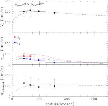
Figure 1: Derived circular velocity and the components of the velocity dispersion versus radius for the model galaxy in the disk and in the bulge, for $437$ particles, upper panel, and $136$ particles, bottom panel.The filled symbols are from the maximum-likelihood analysis, with vertical error bars indicating uncertainty and horizontal error bars showing the extent of each radial bin (with the point plotted at the median radius for a PN in that bin). The dashed lines represent the model circular velocity, velocity dispersion in the disk and in the spheroid.

In a simulated galaxy, we have access to inside information which allows us to test specific aspects of this modeling process. In particular, the “stars” are tagged according to whether they are members of the disk or spheroid, so we can assign the objects to specific components with certainty, rather than using the probabilistic approach described above. Accordingly, we have carried out the likelihood analysis without the probabilistic decomposition, with the results presented in Figure 1. The upper panel shows the results obtained with a generous catalogue of 437 objects, while the lower panel shows how well we can do with only 136 kinematic tracers. Although not strictly valid for kinematically-hot S0 galaxies, an asymmetric drift correction has been applied to convert the derived rotation velocity into a circular velocity for direct comparison with the simulation’s known functional form, using the formula

$$V_{c}^{2}=V^{2}+\sigma_{\phi}^{2}-\sigma_{r}^{2}\left(1-{r_{h}\over r_{D}}+\frac{d\ln\sigma_{r}^{2}}{d\ln r}\right),$$ (8)

where $V_{c}$ is the circular velocity, $r_{h}$ is the median radius in each bin, and $r_{D}$ is the disk scale length (Kormendy, 1984). The final gradient term of the equation has been estimated assuming that $\sigma_{r}^{2}$ follows an exponential profile and performing a linear fit between $\ln\sigma_{r}^{2}$ and the radius.

While the errors are, as expected, larger for the smaller sample, there are no systematic differences between them, and both do a good job of recovering the simulation’s circular velocity. It is interesting to see that $\sigma_{R}$ is moderately but systematically too low for the small sample-size, and remains low at large radii even for the larger sample. Since the main remaining assumption in this model is that the velocity distributions of the individual components are intrinsically Gaussian, it seems likely that this modest systematic error occurs due to the breakdown of this assumption. However, we note that $\sigma_{\phi}$ and $v$ are both quite accurately recovered, so we can estimate with some confidence the balance between random and rotational motion, $\sigma_{\phi}/v$, which is the main physical quantity that we are seeking to use as a diagnostic in this analysis of the origins of S0 galaxies.

3.2 Testing the effect of the photometric spheroid–disk decomposition

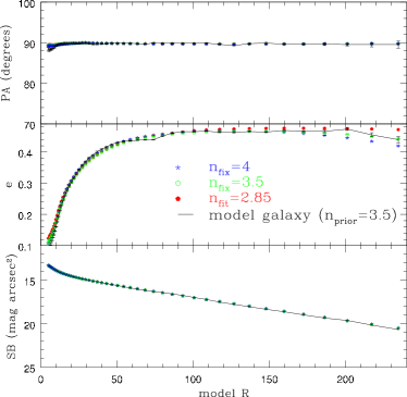
Figure 2: Results from the isophotal analysis of the simulated galaxy, black filled triangles, and the galaxy models obtained with GALFIT leaving the Sersic index $n$ as a free parameter, red filled pentagons, imposing $S_{GALFIT}=3.5$, green open pentagons and imposing $S_{GALFIT}=4$, blue starred symbols. The top row shows the fitted position angles, the middle row the ellipticity and the bottom row the surface brightness.

We now introduce the remaining aspect of the full model-fitting process, the spheroid–disk decomposition, which allows us to assign a probabilistic membership of each kinematic tracer to each component, since, as discussed above, in a real galaxy we do not have the luxury of this knowledge a priori. We constructed an image of the simulated galaxy and convolved it with a suitable Gaussian point-spread function. We then used GALFIT to model the resulting simulated broad-band image. The principal parameters returned by this fitting process are the spheroid and disk magnitudes, their respective scale lengths, the Sersic index of the spheroid, and the flattening and position angle of the components.

Interestingly, if the parameters are all left free, then the spheroid is found to have a best-fit Sersic index of 2.8, significantly smaller than the known value for this simulation of 3.5. The value of the effective radius is also found to be systematically too small. However, an almost equally-good fit is found if we fix the Sersic index to 3.5. In fact, this fit is by some measures superior: Figure 2 shows the values of position angle, ellipticity and surface brightness obtained by fitting elliptical isophotes to both the simulated galaxy image and the models in which the Sersic index is either fixed or left free. While both models reproduce the position angle and surface brightness equally well, the ellipticity is clearly better fitted by the model with the Sersic index fixed at the right value. This conflicting information underlines the complexity of non-linear model fitting, and illustrates its basic limitations.

Of course, for a real galaxy, we would not know the “right” value for the Sersic index, so would not be able to choose between these models. Such systematic errors in GALFIT fitting therefore pose a potential limitation to the effectiveness of the modeling procedure set out in this paper, if the resulting kinematics turn out to depend sensitively on the spheroid–disk decomposition. To assess the impact of such effects, we carried out the maximum likelihood modeling using both of these decompositions. We also checked the effect of kinematic tracer sample size by simulating catalogues of 437 and 136 PNe. The resulting kinematics are presented in Figure 3. The good news is that the results are largely insensitive to systematic errors arising from the disk – spheroid decomposition. For the smaller catalogue, the extra uncertainty that arises from the decomposition process mean that the errors in the derived kinematic quantities become quite large, but there is no evidence for any systematic error in the process. Thus, it appears that this maximum likelihood procedure is quite reliable, and robust against the most likely sources of systematic error in the spheroid–bulge decomposition.

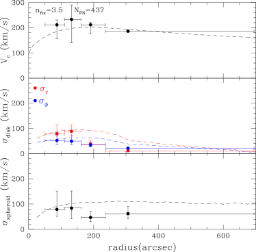
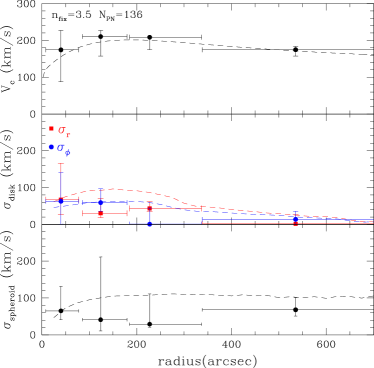
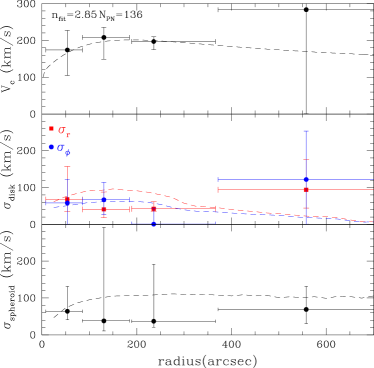
Figure 3: Derived circular velocity and the components of the velocity dispersion versus radius for the model galaxy in the disk and in the bulge. The left panels show the result when the spheroid’s Sersic index is fixed at its true value of 3.5, while the right panels show the results when it is left as a free parameter. Upper panels are for a larger catalogue of 437 kinematic tracers; lower panels for a smaller sample of 136. The filled symbols are from the maximum-likelihood analysis, with vertical error bars indicating uncertainty and horizontal error bars showing the extent of each radial bin (with the point plotted at the median location for a kinematic tracer in that bin).

4 Application to NGC 1023

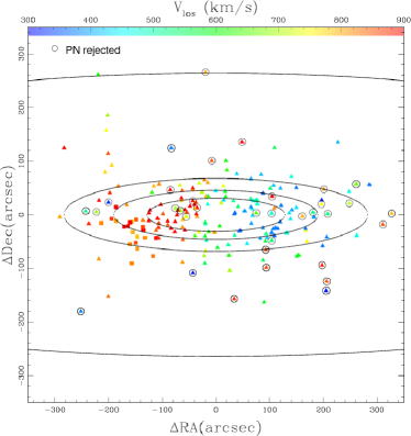
Figure 4: Positions and velocities of the PNe detected in NGC 1023. Colors bar indicates velocities. The elliptical annuli show the radial binning of the data. The circled points are those rejected in the pure disk model, with the likelihood clipping probability threshold increased to $1.65\sigma$. Squares show PNe associated with the companion galaxy NGC 1023A (Noordermeer et al.,, 2008).

Having developed this methodology for extracting kinematic properties of disk galaxies from individual stellar tracers, and tested its reliability, we can now apply it to the existing PNe data for the S0 galaxy NGC 1023. The catalogue of 183 PNe positions and velocities, published by Noordermeer et al., (2008), are presented in Figure 4. Note the “hole” in the middle of the galaxy resulting from the difficulty of detecting PNe against the bright stellar continuum at these radii, as discussed above. Application of the new method to these data has the benefit that they have already been studied using a more conventional tilted-ring model (Noordermeer et al.,, 2008), with which our results can be compared, plus the somewhat peculiar kinematics apparently found in this system warrant further investigation. Since the previous analysis by Noordermeer et al., (2008) neglected any contribution to the kinematics from the bulge, we begin by considering the disk-only model to make a direct comparison.

4.1 The disk model

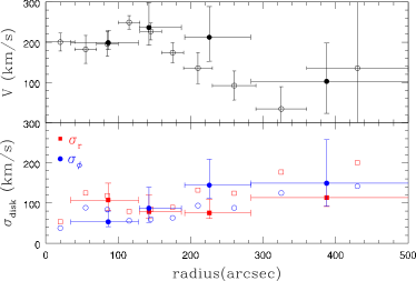
Figure 5: Derived mean rotation speed and the components of the velocity dispersion versus radius for NGC 1023, for the case of a disk-only model. The filled symbols are from the maximum-likelihood analysis, with vertical error bars indicating uncertainty and horizontal error bars showing the extent of each radial bin (with the point plotted at the median location for a PN in that bin). The open symbols reproduce the results of the tilted-ring analysis by Noordermeer et al., (2008).

The application of the above approach, in which the data are binned radially (into the annuli indicated in Figure 4) but modeled azimuthally by likelihood analysis, is presented in Figure 5. For this analysis and the following sections, we have estimated the galaxy’s inclination from the ellipticity of the disk component derived from the two-dimensional fit to the photometry (see Section 4.2); assuming that the disk is intrinsically axisymmetric, we infer a value of $i=74.3$ degrees. Likelihood clipping has been applied such that PNe with a probability of less than $2.1\sigma$ of being drawn from the disk model are rejected. As is clear from this figure, the analysis largely reproduces the peculiar result of Noordermeer et al., (2008), with an inferred rotation speed that falls rapidly outside 300 arcseconds, accompanied by a rise in velocity dispersion. As previously noted, such kinematics were not predicted by any of the simpler scenarios for S0 formation, therefore motivating this further investigation.

One immediate clue is offered by the only significant difference between the results of the two analyses presented in Figure 5. Specifically, while the radial dispersion exceeds the tangential component in the Noordermeer et al., (2008) analysis, the opposite is the case in the maximum likelihood fit. In fact, the ordering of dispersions was fixed in the first analysis, as their ratio was set by the epicyclic approximation, which forces $\sigma_{r}>\sigma_{\phi}$ unless the rotation curve is very rapidly rising (Binney & Tremaine,, 1987). In the current analysis, we have left both components as free parameters, and it is telling us that we then find $\sigma_{\phi}>\sigma_{r}$, which is not what the physically-motivated epicyclic approximation would produce, suggesting that there is some basic flaw in the model.

As noted above, the principal missing element in this model is the spheroidal component, which is consistent with the enhanced value of $\sigma_{\phi}$. Specifically, a spheroid will contribute a relatively small number of PNe with a large dispersion but zero mean velocity. Close to the minor axis of the galaxy, the disk PNe will also have zero mean line-of-sight velocity, whereas on the major axis their distribution will be offset in velocity due to rotation. Combining the two distributions with different mean velocities will result in a larger incorrectly-inferred dispersion than combining them where their mean velocities are the same. Since the tangential component projects mostly into the line-of-sight close to the major axis, its derived value would be more enhanced by this contamination than that of the radial component, consistent with the results in Figure 5.

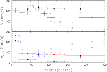
Figure 6: As for Figure 5, but with the likelihood clipping probability threshold increased to $1.65\sigma$.

A very simple test of whether such contamination could be responsible for the unphysical results can be made by increasing the severity of the likelihood clipping, to try to remove the contaminants from the fit. Figure 6 shows the success of such a process, in which a more aggressive threshold resulted in 34 PNe being rejected. The components of the velocity dispersions are now ordered in the manner physically expected for a disk population. Further, the bizarre behavior of the kinematics has entirely vanished, with the rotation velocity now remaining approximately constant out to large radii, and the dispersion remaining low, just as one would expect for a normal disk population.

As further evidence that the cause of the contamination is the spheroid, Figure 4 highlights the locations of the PNe rejected in this iterative clipping. The PNe appear spread throughout the galaxy, and not flattened into the aspect ratio of the disk, indicating that they are probably not the result of a poor disk model. There is, however, some indication of an asymmetry in rejected PNe between the two sides of the galaxy, which we return to in Section 4.4.

Clearly we need to model a spheroidal component as well as the disk, but it is also heartening to see that the likelihood rejection method does a respectable job of dealing with even such a high level of contamination, in which almost $20\%$ of the PNe do not seem to be drawn from the assumed model. This result provides some confidence in the robustness of the adopted procedure.

4.2 Spheroid – disk decomposition

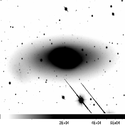
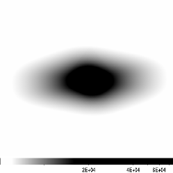
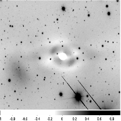
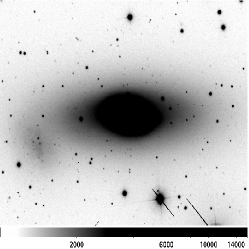
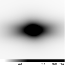
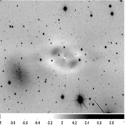
Figure 7: GALFIT analysis of NGC 1023. The top row is for a R-band image; the bottom row is for an B-band image. The data are obtained with the Isaac Newton Telescope on 1995 December 25, using the prime focus camera. The $300$ second exposures cover a field of view of $10.2^{\prime}\times 10.2^{\prime}$ (Noordermeer et al.,, 2008). The first column shows the original data, the second column presents the model, and the third column shows the result of subtracting the model from the data. The residual image has been normalized by the original data, so that the values range from $0$ for a perfect fit, to $1$ or $-1$, where the data has not been fitted at all.

The first step toward modeling the spheroidal component is to decompose continuum images into disk and spheroidal components, which we have done using GALFIT (Peng et al.,, 2002) to fit an exponential disk and a de Vaucouleurs law spheroid to deep images of NGC 1023. Figure 7 shows the result of this process carried out on both B and R band images. The companion galaxy NGC 1023A is mildly apparent even in the raw images, but shows up very clearly in the residuals when the model is subtracted. The residual image also shows evidence for the bar at the centre of this galaxy noted by Debattista et al., (2002); since this faint feature is relatively localized at small radii, and we are primarily interested in the balance between disk and spheroid light at large radii, we do not attempt to model it any further. We could also have considered other models for the spheroid, such as incorporating distinct bulge and halo components, or picking a more general Sersic profile for the light distribution. However, as we have seen in Section 3, the results are relatively insensitive to such subtleties. Since the primary goal is just to model to a reasonable approximation the fraction of the light in the different components at different positions, there is little benefit in trying to distinguish between what are likely to be near-degenerate alternative fits.

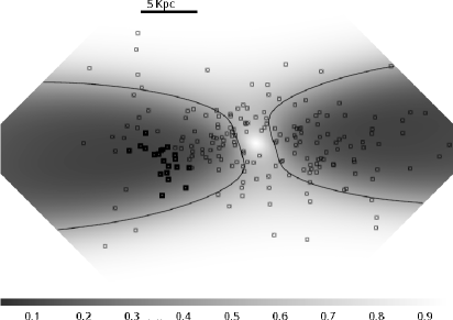
Figure 8: Map showing the probability, $f$, that a PN at any given location is drawn from the spheroidal component of NGC 1023. The positions of the detected PNe are superimposed. Bold squares identify NGC1023A PNe. The $f=0.5$ contour is shown in black.

From the models in the two bands, we can calculate colors for the individual components, and in this case we find $B-R=1.62$ for the disk and $1.61$ for the spheroid. Thus there appears to be essentially no color difference between the components. We also find no significant difference between the scale-lengths of the components in the two bands: the best-fit model disk has a scale length of 67 arcseconds for the B-band data and 66 arcseconds for the R-band; similarly, the spheroid has an effective radius of 24 arcseconds in the B-band and 21 arcseconds in the R-band. There is thus no evidence for color gradients within each component. This lack of color variation between and within components makes the translation from stellar continuum properties to the probability that a PN belongs to the spheroid or disk particularly simple in this case, as the probability is just the ratio of the component to total light at each point. The bulge to total light ratio is 0.31 in the R-band and 0.35 in the B-band. These values compare well with estimates from the cruder one-dimensional bulge–disk light decomposition performed in (Noordermeer et al.,, 2008), where the bulge-to-total light ratio was found to be 0.36. The two-dimensional map of the fraction of light in the spheroidal component, $f$, as a function of position on the sky is presented in Figure 8. As discussed in Section 2.3, the value of $f$ clearly varies strongly with azimuth, with the spheroid being the dominant component at all radii close to the minor axis, underlining the necessity of this full two-dimensional decomposition.

4.3 The disk $+$ spheroid model

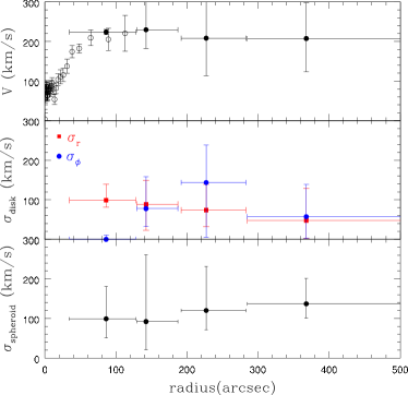
Figure 9: Derived mean rotation speed, the components of the disk velocity dispersion, and the spheroid dispersion versus radius for NGC 1023. The filled symbols are from the maximum-likelihood analysis, with vertical error bars indicating uncertainty and horizontal error bars showing the extent of each radial bin (with the point plotted at the median location for a PN in that bin. The open symbols show rotation velocities derived from absorption-line data by Debattista et al., (2002).

Having calculated the division between spheroid and disk light, we can now carry out the likelihood analysis for NGC 1023 incorporating this extra component, as set out in Section 2.2. the resulting best-fit kinematic parameters as a function of radius are shown in Figure 9. We now start to see the characteristic properties of a normal disk galaxy. Rotation dominates random motions in the disk at all radii, and the mean rotation speed stays approximately constant out to the last points shown. In this plot, we have also filled in the missing stellar rotation velocity at small radii from conventional absorption-line data, and it is clear that the two techniques agree extremely well where they overlap. The spheroid dispersion profile is also very well-behaved, showing little if any variation with radius (justifying the compromise in radial binning discussed in Section 2.2). It is also notable that the approximately-constant spheroid dispersion is consistent with a value of $V/\sqrt{2}$, which is what one would obtain for the simplest possible model of a singular isothermal sphere potential, in which circular speed and velocity dispersion are related in this way. This consistency is reassuring, as the fitting procedure in no way imposed it on the results.

As one further enhancement, one might also expect some rotational velocity, $V_{s}$, in the spheroidal component, which might affect the results. Indeed, there is known to be a strong correlation between ellipticity and rotational speed in low-luminosity spheroidal systems like this bulge (see Figure 4.14 in Binney & Tremaine,, 1987). The GALFIT modeling shows that the spheroid in NGC 1023 has an ellipticity of $\sim 0.25$, which translates into a predicted value of $V_{s}/\sigma_{s}\sim 0.5$. We have experimented with including rotation at this level in the spheroidal component by modifying the first term in Equation 7, but find that at this level the inclusion of rotation makes no significant difference to the remaining kinematic parameters.

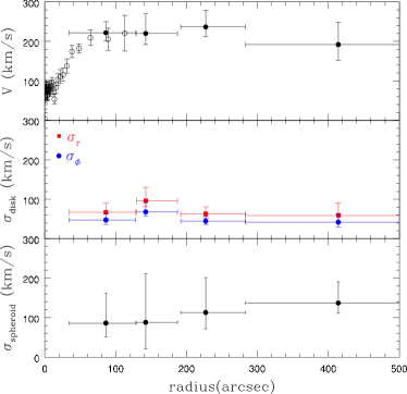
Figure 10: As for Figure 9, but with the ratio of disk dispersions components constrained by the epicyclic approximation.

The only slight disappointment in the fitting process is that the ratio between the components of disk dispersion is somewhat less well defined than was the case in the disk-only model fit, which presumably reflects the impact of the extra spheroidal dispersion free parameter in this model. However, now that we clearly have a well-behaved normal disk system in this galaxy, it seems reasonable to reduce the number of free parameters by invoking the epicyclic approximation. In particular, for such a cold disk system with a flat rotation curve, we expect $\sigma_{\phi}/\sigma_{r}=1/\sqrt{2}$. With this additional constraint, we obtain the kinematic parameters plotted in Figure 10. The error bars on all parameters are duly reduced, and we now find that the kinematics of NGC 1023 are exactly what one would expect for a very normal disk galaxy, with $V/\sigma_{\phi}\simeq 4.1$ throughout the disk, similar to what one finds in the stellar component of a spiral galaxy. Thus, we seem to have found the explanation for the strange kinematics originally inferred from these data for NGC 1023, and it is now revealed to be most likely a spiral galaxy that has simply been stripped of its gas.

4.4 PNe objects rejections: the footprint of an ongoing merger

Figure 11: Plot of radial velocity versus right ascension for the PNe in NGC 1023. Filled symbols show the objects rejected by the likelihood clipping in the full disk+spheroid model. Asterisks show the PNe attributed to NGC 1023A.

However, the story does not quite finish there. Even with the full disk+spheroid kinematic model, 17 PNe are still likelihood-clipped at a threshold probability of $2.1\sigma$. In Figure 11, we show the locations of the PNe in both velocity and right ascension, with the rejected objects highlighted. Since NGC 1023 lies at a position angle very close to 90 degrees, the spatial coordinate is essentially the distance along the major axis, so this is a conventional position–velocity diagram, with the usual antisymmetric signature of a rotating disk evident in the PNe. The rejected PNe, however, do not show such antisymmetry, with the vast majority located on one side of the galaxy. Such an asymmetric arrangement is clearly not consistent with errors arising from a poor choice for any axisymmetric element in the model, or from mis-identified unrelated background objects.

A clue to their origin comes from considering the location of NGC 1023A in this plot, as the rejected PNe seem almost all to form a continuous stream that passes through this companion galaxy, as one might expect if the systems are tidally interacting Capaccioli et al. (1986). It therefore seems likely that these PNe lie in the tidal debris from this companion as it is stripped in an on-going minor merger.

5 Conclusions

We have presented a new method for analyzing the kinematics of disk galaxies as derived from individual stellar tracers such as PNe. This hybrid technique bins data radially in the galaxy to maintain the maximum flexibility in the inferred kinematics, but uses a likelihood analysis within each bin so as to derive the maximum amount of information from the discrete data points. In addition, we use photometric decomposition of continuum images to assign a probability to each kinematic tracer of belonging to either the disk or the spheroidal component of the galaxy being modeled.

Application of the method to simulated data shows that it reproduces most of the intrinsic dynamics of a galaxy even when the number of discrete kinematic data points is relatively modest. Application of this technique to NGC 1023 has offered an explanation for the strange kinematics previously inferred for this system. These peculiar properties can be entirely attributed to uncorrected contamination by the galaxy’s spheroidal component, and when this element is properly modeled, the galaxy is revealed to have stellar kinematics entirely consistent with a normal spiral system, with a cold rotationally-supported disk and a hot spheroid with the expected velocity dispersion. This result favours a model in which NGC 1023 formed from a spiral via a simple gas stripping process or secular evolution, rather than through a more disruptive minor merger.

One benefit of the likelihood analysis made clear by this application is that it is possible to “likelihood clip”, to identify objects that do not seem to be drawn from the model, in a reasonably robust and objective manner. Comparison of Figures 10 and 6 shows that such clipping can deal quite well with even the rather extreme case where only the disk is included in the model. Where a more realistic disk+spheroid model is adopted, it seems to do a good job of identifying features like stellar streams, adding to our understanding of the dynamical properties of such systems.

Clearly, though, although the detailed dynamics of this galaxy are interesting, one cannot infer any general conclusions about the formation of S0 galaxies from a single object. Therefore, the next step in this project will involve applying this analysis technique to observations of a larger sample of S0 galaxies whose PNe kinematics have been observed with PN.S. By obtaining a measure of the stellar kinematics of S0s in regions spanning a range of galaxy densities, we will be able to see if they all have the stripped-spiral properties of NGC 1023, and hence whether there is a single route to S0 formation irrespective of environment.

References

- Aragón-Salamanca, (2008) Aragón-Salamanca, A. 2008, IAU Symposium, 245, 285
- Binney & Merrifield, (1998) Binney, J., & Merrifield, M. 1998, Galactic astronomy / James Binney and Michael Merrifield. Princeton, NJ : Princeton University Press.
- Binney & Tremaine, (1987) Binney, J., & Tremaine, S. 1987, Princeton, NJ, Princeton University Press, 1987, 747 p.,
- Bournaud et al., (2005) Bournaud, F., Jog, C. J., & Combes, F. 2005, A&A, 437, 69
- Buzzoni et al., (2006) Buzzoni, A., Arnaboldi, M., & Corradi, R. L. M. 2006, MNRAS, 368, 877
- Capaccioli et al. (1986) Capaccioli, M., Lorenz, H., & Afanasjev, V. L. 1986, A&A, 169, 54
- Ciardullo et al., (1989) Ciardullo, R., Jacoby, G. H., Ford, H. C., & Neill, J. D. 1989, ApJ, 339, 53
- Ciardullo et al., (1991) Ciardullo, R., Jacoby, G. H., & Harris, W. E. 1991, ApJ, 383, 487
- Ciardullo et al., (2002) Ciardullo, R., Feldmeier, J. J., Jacoby, G. H., Kuzio de Naray, R., Laychak, M. B., & Durrell, P. R. 2002, ApJ, 577, 31
- Coccato et al. (2009) Coccato, L., et al. 2009, MNRAS, 394, 1249
- Debattista et al., (2002) Debattista, V. P., Corsini, E. M., & Aguerri, J. A. L. 2002, MNRAS, 332, 65
- Douglas et al., (2002) Douglas, N. G., et al. 2002, PASP, 114, 1234
- Jacoby, (1980) Jacoby, G. H. 1980, ApJS, 42, 1
- Kormendy (1984) Kormendy, J. 1984, ApJ, 286, 116
- Kuijken & Dubinski (1995) Kuijken, K., & Dubinski, J. 1995, MNRAS, 277, 1341
- Merrett et al. (2003) Merrett, H. R., et al. 2003, MNRAS, 346, L62
- Merrett et al. (2006) Merrett, H., et al. 2006, MNRAS, 369, 120
- Morganti et al., (2006) Morganti, R., et al. 2006, MNRAS, 371, 157
- Napolitano et al. (2001) Napolitano, N. R., Arnaboldi, M., Freeman, K. C., & Capaccioli, M. 2001, A&A, 377, 784
- Napolitano et al. (2009) Napolitano, N. R., et al. 2009, MNRAS, 393, 329
- Noordermeer et al., (2008) Noordermeer, E.; Merrifield, M. R.; Coccato, L.; Arnaboldi, M.; Capaccioli, M.; Douglas, N. G.; Freeman, K. C.; Gerhard, O.; Kuijken, K.; de Lorenzi, F.; Napolitano, N. R.; Romanowsky, A. J., 2008, MNRAS, 384, 943
- Noordermeer et al., (2008) Noordermeer, E., Merrifield, M. R., & Aragón-Salamanca, A. 2008, MNRAS, 388, 1381
- Peng et al., (2002) Peng, C. Y., Ho, L. C., Impey, C. D., & Rix, H.-W. 2002, AJ, 124, 266
- Romanowsky et al. (2003) Romanowsky, A. J., Douglas, N. G., Arnaboldi, M., Kuijken, K., Merrifield, M. R., Napolitano, N. R., Capaccioli, M., & Freeman, K. C. 2003, Science, 301, 1696
- Scorza & Bender, (1995) Scorza, C., & Bender, R. 1995, A&A, 293, 20
- Widrow et al. (2008) Widrow, L. M., Pym, B., & Dubinski, J. 2008, ApJ, 679, 1239
- Williams et al. (2010) Williams, M. J., Bureau, M., & Cappellari, M. 2010, MNRAS, 1336