Mean first-passage time of surface-mediated diffusion in spherical domains

O. Bénichou Laboratoire de Physique Théorique de la Matière Condensée (UMR 7600), case courrier 121, Université Paris 6, 4 Place Jussieu, 75255 Paris Cedex    D. S. Grebenkov Laboratoire de Physique de la Matière Condensée (UMR7643), CNRS – Ecole Polytechnique, F-91128 Palaiseau Cedex France Laboratoire Poncelet (UMI 2615), CNRS – Independent University of Moscow, Bolshoy Vlasyevskiy Pereulok 11, 119002 Moscow, Russia    P. E. Levitz Laboratoire de Physique de la Matière Condensée (UMR7643), CNRS – Ecole Polytechnique, F-91128 Palaiseau Cedex France    C. Loverdo Laboratoire de Physique Théorique de la Matière Condensée (UMR 7600), case courrier 121, Université Paris 6, 4 Place Jussieu, 75255 Paris Cedex    R. Voituriez Laboratoire de Physique Théorique de la Matière Condensée (UMR 7600), case courrier 121, Université Paris 6, 4 Place Jussieu, 75255 Paris Cedex
Abstract

We present an exact calculation of the mean first-passage time to a target on the surface of a 2D or 3D spherical domain, for a molecule alternating phases of surface diffusion on the domain boundary and phases of bulk diffusion. The presented approach is based on an integral equation which can be solved analytically. Numerically validated approximation schemes, which provide more tractable expressions of the mean first-passage time are also proposed. In the framework of this minimal model of surface-mediated reactions, we show analytically that the mean reaction time can be minimized as a function of the desorption rate from the surface.

I Introduction

The kinetics of many chemical reactions is influenced by the transport properties of the reactants that they involve Rice (1985); Hänggi et al. (1990). In fact, schematically, any chemical reaction requires first that a given reactant A meets a second reactant B. This first reaction step can be rephrased as a search process involving a searcher A looking for a target B. In a very dilute regime, exemplified by biochemical reactions in cells Alberts et al. (2002) which sometimes involve only a few copies of reactants, the targets B are sparse and therefore hard to find in this search process language. In such reactions, the first step of search for reactants B is therefore a limiting factor of the global reaction kinetics. In the general aim of enhancing the reactivity of chemical systems, it is therefore needed to optimize the efficiency of this first step of search.

Recently, it has been shown that intermittent processes, combining slow diffusion phases with a faster transport, can significantly increase reactions rates Benichou et al. (2005, 2008). A minimal model demonstrating the efficiency of this type of search, introduced to account for the fast search of target sequences on DNA by proteins Coppey et al. (2004) is as follows (see also Berg et al. (1981); Slutsky and Mirny (2004); Lomholt et al. (2005); Eliazar et al. (2007)). The pathway followed by the protein, considered as a point-like particle, is a succession of 1D diffusions along the DNA strand (called sliding phases) with diffusion coefficient D1subscript𝐷1D_{1} and 3D excursions in the surrounding solution. The time spent by the protein on DNA during each sliding phase is assumed to follow an exponential law with dissociation rate λ𝜆\lambda. In this minimal model, the 3D excursions are uncorrelated in space, which means that after dissociation from DNA, the protein will rebind the DNA at a random position independently of its starting position. Assuming further that the mean duration of such 3D excursions τ2subscript𝜏2\tau_{2} is finite, it has been shown that the mean first-passage time at the target can be minimized as a function of τ1=λ1subscript𝜏1superscript𝜆1\tau_{1}=\lambda^{-1}, as soon as the mean time spent in bulk excursions is not too long. Quantitatively, this condition writes in orders of magnitude as τ2L2/D1subscript𝜏2superscript𝐿2subscript𝐷1\tau_{2}\leq L^{2}/D_{1}, and the minimum of the search time is obtained for τ1τ2similar-to-or-equalssubscript𝜏1subscript𝜏2\tau_{1}\simeq\tau_{2} in the large L𝐿L limit. Note that in this minimal model, where the time τ2subscript𝜏2\tau_{2} is supposed to be a fixed exterior parameter, bulk phases are always beneficial in the large L𝐿L limit (i.e. allow one to decrease the search time with respect to the situation corresponding to 1D diffusion only).

In many practical situations however, the duration of the fast bulk excursions strongly depends on the geometrical properties of the system Bénichou et al. (2005); Levitz et al. (2006); Chechkin et al. (2009); Loverdo et al. (2009) and cannot be treated as an independent variable as assumed in the mean-field (MF) model introduced above. An important generic situation concerns the case of confined systems Astumian and Chock (1985); Adam and Delbrück (1968); Sano and Tachiya (1981), involving transport of reactive molecules both in the bulk of a confining domain and on its boundary, referred to as surface-mediated diffusion in what follows. This type of problems is met in situations as varied as heterogeneous catalysis Bond (1987); Blumen et al. (1984), or reactions in porous media and in vesicular systems Adam and Delbrück (1968); Sano and Tachiya (1981); Schuss et al. (2007). In all these examples, the duration of bulk excursions is controlled by the return statistics of the molecule to the confining surface, which crucially depends on the volume of the system. This naturally induces strong correlations between the starting and ending points of bulk excursions, and makes the above MF assumption of uncorrelated excursions largely inapplicable in these examples.

At the theoretical level, the question of determining mean first-passage times in confinement has attracted a lot of attention in recent years for discrete random walks Kozak and Balakrishnan (2002); Condamin et al. (2007b); Agliari (2008); Haynes and Roberts (2008); Reuveni et al. (2010) and continuous processes Redner (2001); Condamin et al. (2005); Grebenkov (2007); Condamin et al. (2007). More precisely, the surface-mediated diffusion problem considered here generalizes the so-called narrow escape problem, which refers to the time needed for a simple Brownian motion in absence of surface diffusion to escape through a small window of an otherwise reflecting domain. This problem has been investigated both in the mathematical Singer et al. (2006a); Schuss et al. (2007); Pillay et al. (2010); Cheviakov et al. (2010) and physical Grigoriev et al. (2002); Benichou and Voituriez (2008); Oshanin et al. (2010); Chevalier et al. (2011) literature, partly due to the challenge of taking into account mixed boundary conditions. The case of surface-mediated diffusion brings the additional question of minimizing the search time with respect to the time spent in adsorption, in the same spirit as done for intermittent processes introduced above. The answer to this question is a priori not clear, since the mean time spent in bulk excursions diverges for large confining domains, so that the condition of minimization mentioned previously cannot be taken as granted, even in the large system limit. In this context, first results have been obtained in Bénichou et al. (2010) where, surprisingly enough, it has been found that, even for bulk and surface diffusion coefficients of the same order of magnitude, the reaction time can be minimized, whereas MF treatments (see for instance Oshanin et al. (2010)) predict a monotonic behavior.

Here, we extend the perturbative results of Bénichou et al. (2010) obtained in the small target size limit. Relying on an integral equation approach, we provide an exact solution for the mean FPT, both for 2D an 3D spherical domains, and for any spherical target size. We also develop approximation schemes, numerically validated, that provide more tractable expressions of the mean FPT.

II The model

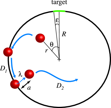
The surface-mediated process under study is defined as follows. We consider a molecule diffusing in a spherical confining domain of radius R𝑅R (see figure 1), alternating phases of boundary diffusion (with diffusion coefficient D1subscript𝐷1D_{1}) and phases of bulk diffusion (with diffusion coefficient D2subscript𝐷2D_{2}). The time spent during each one-dimensional phase is assumed to follow an exponential law with dissociation rate λ𝜆\lambda. At each desorption event, the molecule is assumed to be ejected at a distance a𝑎a from the frontier (otherwise it is instantaneously readsorbed). Although formulated for any value of this parameter a𝑎a smaller than R𝑅R, in most physical situations of real interest aRmuch-less-than𝑎𝑅a\ll R. The target is perfectly absorbing and defined in 2D2𝐷2D by the arc θ[ϵ,ϵ]𝜃italic-ϵitalic-ϵ\theta\in[-\epsilon,\epsilon], and in 3D3𝐷3D by the region of the sphere such that θ[0,ϵ]𝜃0italic-ϵ\theta\in[0,\epsilon] where θ𝜃\theta is in this case the elevation angle in standard spherical coordinates. Note that as soon as ϵ0italic-ϵ0\epsilon\neq 0, the target can be reached either by surface or bulk diffusion. In what follows we calculate the mean first-passage time at the target for an arbitrary initial condition of the molecule.
Refer to caption
Figure 1: Model

III 2D case

In this section, the confining domain is a disk of radius R𝑅R and the target is defined by the arc θ[ϵ,ϵ]𝜃italic-ϵitalic-ϵ\theta\in[-\epsilon,\epsilon].

III.1 Basic equations

For the process defined above, the mean first-passage time (MFPT) at the target satisfies the following backward equations

D1R2t1′′(θ)+λ[t2(Ra,θ)t1(θ)]subscript𝐷1superscript𝑅2superscriptsubscript𝑡1′′𝜃𝜆delimited-[]subscript𝑡2𝑅𝑎𝜃subscript𝑡1𝜃\displaystyle\frac{D_{1}}{R^{2}}t_{1}^{\prime\prime}(\theta)+\lambda[t_{2}(R-a,\theta)-t_{1}(\theta)] =\displaystyle= 1forθ[ϵ,2πϵ],1for𝜃italic-ϵ2𝜋italic-ϵ\displaystyle-1\;\;{\rm for}\;\theta\in[\epsilon,2\pi-\epsilon], (1)
D2(2r2+1rr+1r22θ2)t2(r,θ)subscript𝐷2superscript2superscript𝑟21𝑟𝑟1superscript𝑟2superscript2superscript𝜃2subscript𝑡2𝑟𝜃\displaystyle D_{2}\left(\frac{\partial^{2}}{\partial r^{2}}+\frac{1}{r}\frac{\partial}{\partial r}+\frac{1}{r^{2}}\frac{\partial^{2}}{\partial\theta^{2}}\right)t_{2}(r,\theta) =\displaystyle= 1,1\displaystyle-1, (2)

where t1subscript𝑡1t_{1} stands for the the MFPT starting from the circle at a position defined on the circumference by the angle θ𝜃\theta, and t2subscript𝑡2t_{2} for the MFPT starting from the point (r,θ)𝑟𝜃(r,\theta) within the disk. In these two equations, the first term of the lhs accounts for the diffusion respectively on the circumference and in the bulk, while the second term of Eq. (1) describes desorption events. They have to be completed by two boundary conditions

t2(R,θ)subscript𝑡2𝑅𝜃\displaystyle t_{2}(R,\theta) =\displaystyle= t1(θ),subscript𝑡1𝜃\displaystyle t_{1}(\theta), (3)
t1(θ)subscript𝑡1𝜃\displaystyle t_{1}(\theta) =\displaystyle= 0forθ[0,ϵ][2πϵ,2π],0for𝜃0italic-ϵ2𝜋italic-ϵ2𝜋\displaystyle 0\;\;{\rm for}\;\theta\in[0,\epsilon]\cup[2\pi-\epsilon,2\pi], (4)

which describe the adsorption events and the absorbing target respectively. Eq.(2) is easily shown to be satisfied by the following Fourier series

t2(r,θ)=α0r24D2+n=1αnrncos(nθ),subscript𝑡2𝑟𝜃subscript𝛼0superscript𝑟24subscript𝐷2superscriptsubscript𝑛1subscript𝛼𝑛superscript𝑟𝑛𝑛𝜃t_{2}(r,\theta)=\alpha_{0}-\frac{r^{2}}{4D_{2}}+\sum_{n=1}^{\infty}\alpha_{n}r^{n}\cos(n\theta), (5)

with unknown coefficients αnsubscript𝛼𝑛\alpha_{n} to be determined. In particular, we aim at determining the search time t1delimited-⟨⟩subscript𝑡1\langle t_{1}\rangle, defined as the MFPT, with an initial position uniformly distributed on the boundary of the confining domain. Taking Eq.(5) at r=R𝑟𝑅r=R, we have

α0R24D2+n=1αnRncos(nθ)={t1(θ)if θ[ϵ,2πϵ],0if θ[0,ϵ][2πϵ,2π],subscript𝛼0superscript𝑅24subscript𝐷2superscriptsubscript𝑛1subscript𝛼𝑛superscript𝑅𝑛𝑛𝜃casessubscript𝑡1𝜃if θ[ϵ,2πϵ],0if θ[0,ϵ][2πϵ,2π],\alpha_{0}-\frac{R^{2}}{4D_{2}}+\sum_{n=1}^{\infty}\alpha_{n}R^{n}\cos(n\theta)=\begin{cases}t_{1}(\theta)&\text{if $\theta\in[\epsilon,2\pi-\epsilon]$,}\\ 0&\text{if $\theta\in[0,\epsilon]\cup[2\pi-\epsilon,2\pi]$,}\end{cases} (6)

so that

α0R24D2=12πϵ2πϵt1(θ)dθt1,Rnαn=1πϵ2πϵt1(θ)cos(nθ)dθ(n1).formulae-sequencesubscript𝛼0superscript𝑅24subscript𝐷212𝜋superscriptsubscriptitalic-ϵ2𝜋italic-ϵsubscript𝑡1𝜃differential-d𝜃delimited-⟨⟩subscript𝑡1superscript𝑅𝑛subscript𝛼𝑛1𝜋superscriptsubscriptitalic-ϵ2𝜋italic-ϵsubscript𝑡1𝜃𝑛𝜃differential-d𝜃𝑛1\begin{split}\alpha_{0}-\frac{R^{2}}{4D_{2}}&=\frac{1}{2\pi}\int_{\epsilon}^{2\pi-\epsilon}t_{1}(\theta){\rm d}\theta\equiv\langle t_{1}\rangle,\\ R^{n}\alpha_{n}&=\frac{1}{\pi}\int_{\epsilon}^{2\pi-\epsilon}t_{1}(\theta)\cos(n\theta){\rm d}\theta\hskip 14.22636pt(n\geq 1).\\ \end{split} (7)

In what follows we will make use of the following quantities:

ωRλ/D1,𝜔𝑅𝜆subscript𝐷1\omega\equiv R\sqrt{\lambda/D_{1}}, (8)
x1aR,𝑥1𝑎𝑅x\equiv 1-\frac{a}{R}, (9)

and

T1λ+R2(Ra)24D2.𝑇1𝜆superscript𝑅2superscript𝑅𝑎24subscript𝐷2T\equiv\frac{1}{\lambda}+\frac{R^{2}-(R-a)^{2}}{4D_{2}}. (10)

As we proceed to show, two different approaches can be used to solve this problem. (i) The first approach, whose main results have been published in Bénichou et al. (2010), uses the explicit form of the Green function for the two-dimensional problem and relies on a small target size ϵitalic-ϵ\epsilon expansion. We recall these perturbative results below for the sake of self-consistency and give details of the derivation in Appendix A. (ii) The second approach presented next relies on an integral equation which can be derived for t1subscript𝑡1t_{1}, and leads to an exact non-perturbative solution.

III.2 Perturbative approach

It is shown in Appendix that the Fourier coefficients of t2(r,θ)subscript𝑡2𝑟𝜃t_{2}(r,\theta) as defined in Eq.(5) satisfy an infinite hierarchy of linear equations, which lead to the following small ϵitalic-ϵ\epsilon expansion:

α0=R24D2+ω2T{(2m=11ω2(1xm)+m2)πϵ+(1+2ω2m=11xmω2(1xm)+m2)ϵ2}+,αn=ω2TRn(ω2(1xn)+n2){2+n2ϵ2+}.formulae-sequencesubscript𝛼0superscript𝑅24subscript𝐷2superscript𝜔2𝑇2superscriptsubscript𝑚11superscript𝜔21superscript𝑥𝑚superscript𝑚2𝜋italic-ϵ12superscript𝜔2superscriptsubscript𝑚11superscript𝑥𝑚superscript𝜔21superscript𝑥𝑚superscript𝑚2superscriptitalic-ϵ2subscript𝛼𝑛superscript𝜔2𝑇superscript𝑅𝑛superscript𝜔21superscript𝑥𝑛superscript𝑛22superscript𝑛2superscriptitalic-ϵ2\begin{split}\alpha_{0}&=\frac{R^{2}}{4D_{2}}+\omega^{2}T\left\{\left(2\sum_{m=1}^{\infty}\frac{1}{\omega^{2}\left(1-x^{m}\right)+m^{2}}\right)-\pi\epsilon+\left(1+2\omega^{2}\sum_{m=1}^{\infty}\frac{1-x^{m}}{\omega^{2}\left(1-x^{m}\right)+m^{2}}\right)\epsilon^{2}\right\}+\dots,\\ \alpha_{n}&=\frac{\omega^{2}T}{R^{n}(\omega^{2}(1-x^{n})+n^{2})}\left\{-2+n^{2}\epsilon^{2}+\dots\right\}.\\ \end{split} (11)

Note that Eq.(11) gives in particular the first terms of the perturbative expansion of the search time t1delimited-⟨⟩subscript𝑡1\langle t_{1}\rangle defined in (7) and given in Bénichou et al. (2010). It should be stressed that since the coefficients of ϵksuperscriptitalic-ϵ𝑘\epsilon^{k} of this expansion diverge with ω𝜔\omega, in practice one finds that the range of applicability in ϵitalic-ϵ\epsilon of this expansion is wider for ω𝜔\omega small.

III.3 Integral equation for t1subscript𝑡1t_{1}

In this section, we first show that the resolution of the coupled PDEs (1, 2) amounts to solving an integral equation for t1subscript𝑡1t_{1} only. As we proceed to show, this integral equation can be solved exactly. Writing Eq. (1) as

2t1θ2=R2D1ω2[t2(Ra,θ)t2(R,θ)],superscript2subscript𝑡1superscript𝜃2superscript𝑅2subscript𝐷1superscript𝜔2delimited-[]subscript𝑡2𝑅𝑎𝜃subscript𝑡2𝑅𝜃\frac{\partial^{2}t_{1}}{\partial\theta^{2}}=-\frac{R^{2}}{D_{1}}-\omega^{2}[t_{2}(R-a,\theta)-t_{2}(R,\theta)], (12)

and expanding its right-hand side into a Taylor series leads to

2t1θ2=R2D1ω2k=1(a)kk!(kt2rk)R,θ.superscript2subscript𝑡1superscript𝜃2superscript𝑅2subscript𝐷1superscript𝜔2superscriptsubscript𝑘1superscript𝑎𝑘𝑘subscriptsuperscript𝑘subscript𝑡2superscript𝑟𝑘𝑅𝜃\frac{\partial^{2}t_{1}}{\partial\theta^{2}}=-\frac{R^{2}}{D_{1}}-\omega^{2}\sum_{k=1}^{\infty}\frac{(-a)^{k}}{k!}\left(\frac{\partial^{k}t_{2}}{\partial r^{k}}\right)_{R,\theta}. (13)

Substituting the Fourier representation (5) for t2subscript𝑡2t_{2} into this equation yields

2t1θ2=R2D1ω2(aR2D2a24D2)ω2k=1(a)kk!n=kαnn(n1)(nk+1)Rnkcos(nθ).superscript2subscript𝑡1superscript𝜃2superscript𝑅2subscript𝐷1superscript𝜔2𝑎𝑅2subscript𝐷2superscript𝑎24subscript𝐷2superscript𝜔2superscriptsubscript𝑘1superscript𝑎𝑘𝑘superscriptsubscript𝑛𝑘subscript𝛼𝑛𝑛𝑛1𝑛𝑘1superscript𝑅𝑛𝑘𝑛𝜃\displaystyle\frac{\partial^{2}t_{1}}{\partial\theta^{2}}=-\frac{R^{2}}{D_{1}}-\omega^{2}\left(\frac{aR}{2D_{2}}-\frac{a^{2}}{4D_{2}}\right)-\omega^{2}\sum_{k=1}^{\infty}\frac{(-a)^{k}}{k!}\sum_{n=k}^{\infty}\alpha_{n}n(n-1)\dots(n-k+1)R^{n-k}\cos(n\theta). (14)

Changing the order of summations over n𝑛n and k𝑘k, using the binomial formula and the expression (7) for αnsubscript𝛼𝑛\alpha_{n} give

2t1θ2=R2D1ω2(aR2D2a24D2)ω2πn=1(xn1)cos(nθ)ϵ2πϵcos(nθ)t1(θ)dθ.superscript2subscript𝑡1superscript𝜃2superscript𝑅2subscript𝐷1superscript𝜔2𝑎𝑅2subscript𝐷2superscript𝑎24subscript𝐷2superscript𝜔2𝜋superscriptsubscript𝑛1superscript𝑥𝑛1𝑛𝜃superscriptsubscriptitalic-ϵ2𝜋italic-ϵ𝑛superscript𝜃subscript𝑡1superscript𝜃differential-dsuperscript𝜃\displaystyle\frac{\partial^{2}t_{1}}{\partial\theta^{2}}=-\frac{R^{2}}{D_{1}}-\omega^{2}\left(\frac{aR}{2D_{2}}-\frac{a^{2}}{4D_{2}}\right)-\frac{\omega^{2}}{\pi}\sum_{n=1}^{\infty}(x^{n}-1)\cos(n\theta)\int_{\epsilon}^{2\pi-\epsilon}\cos(n\theta^{\prime})t_{1}(\theta^{\prime}){\rm d}\theta^{\prime}. (15)

This integro-differential equation for t1subscript𝑡1t_{1} can actually easily be transformed into an integral equation for t1subscript𝑡1t_{1}, by integrating successively two times, which leads to

t1(θ)=12(R2D1+ω2(aR2D2a24D2))(θϵ)(2πϵθ)+ω2πn=1(xn1)cos(nθ)cos(nϵ)n2ϵ2πϵcos(nθ)t1(θ)dθ,subscript𝑡1𝜃12superscript𝑅2subscript𝐷1superscript𝜔2𝑎𝑅2subscript𝐷2superscript𝑎24subscript𝐷2𝜃italic-ϵ2𝜋italic-ϵ𝜃superscript𝜔2𝜋superscriptsubscript𝑛1superscript𝑥𝑛1𝑛𝜃𝑛italic-ϵsuperscript𝑛2superscriptsubscriptitalic-ϵ2𝜋italic-ϵ𝑛superscript𝜃subscript𝑡1superscript𝜃differential-dsuperscript𝜃\begin{split}t_{1}(\theta)&=\frac{1}{2}\left(\frac{R^{2}}{D_{1}}+\omega^{2}\left(\frac{aR}{2D_{2}}-\frac{a^{2}}{4D_{2}}\right)\right)(\theta-\epsilon)(2\pi-\epsilon-\theta)\\ &+\frac{\omega^{2}}{\pi}\sum_{n=1}^{\infty}(x^{n}-1)\frac{\cos(n\theta)-\cos(n\epsilon)}{n^{2}}\int_{\epsilon}^{2\pi-\epsilon}\cos(n\theta^{\prime})t_{1}(\theta^{\prime}){\rm d}\theta^{\prime},\\ \end{split} (16)

or equivalently to

ψ(θ)=(θϵ)(2πϵθ)+Ωn=1(xn1)cos(nθ)cos(nϵ)n2ϵ2πϵcos(nθ)ψ(θ)dθ,𝜓𝜃𝜃italic-ϵ2𝜋italic-ϵ𝜃Ωsuperscriptsubscript𝑛1superscript𝑥𝑛1𝑛𝜃𝑛italic-ϵsuperscript𝑛2superscriptsubscriptitalic-ϵ2𝜋italic-ϵ𝑛superscript𝜃𝜓superscript𝜃differential-dsuperscript𝜃\psi(\theta)=(\theta-\epsilon)(2\pi-\epsilon-\theta)+\Omega\sum_{n=1}^{\infty}(x^{n}-1)\frac{\cos(n\theta)-\cos(n\epsilon)}{n^{2}}\int_{\epsilon}^{2\pi-\epsilon}\cos(n\theta^{\prime})\psi(\theta^{\prime}){\rm d}\theta^{\prime}, (17)

where

ψ(θ)2t1(θ)ω2T,𝜓𝜃2subscript𝑡1𝜃superscript𝜔2𝑇\psi(\theta)\equiv\frac{2t_{1}(\theta)}{\omega^{2}T}, (18)

with T𝑇T defined in Eq. (10) and Ωω2πΩsuperscript𝜔2𝜋\Omega\equiv\frac{\omega^{2}}{\pi}. Note that Eq. (17) holds for θ[ϵ,2πϵ]𝜃italic-ϵ2𝜋italic-ϵ\theta\in[\epsilon,2\pi-\epsilon]. When there is no desorption (i.e., λ=0𝜆0\lambda=0), only the first term in Eq. (18) survives, yielding the classical result Redner (2001)

t1(θ)=R2D1(θϵ)(2πϵθ).subscript𝑡1𝜃superscript𝑅2subscript𝐷1𝜃italic-ϵ2𝜋italic-ϵ𝜃t_{1}(\theta)=\frac{R^{2}}{D_{1}}(\theta-\epsilon)(2\pi-\epsilon-\theta). (19)

The same result is obtained for a=0𝑎0a=0, since xn1=(1a/R)n1=0superscript𝑥𝑛1superscript1𝑎𝑅𝑛10x^{n}-1=(1-a/R)^{n}-1=0. The limit a=0𝑎0a=0 is in fact equivalent to the limit λ=0𝜆0\lambda=0 because, after desorption, the particle immediately returns onto the circle (a=0𝑎0a=0) as if it was never desorbed (λ=0𝜆0\lambda=0).

III.4 Exact solution

Iterating the integral equation (17) shows that the solution ψ(θ)𝜓𝜃\psi(\theta) writes for θ[ϵ,2πϵ]𝜃italic-ϵ2𝜋italic-ϵ\theta\in[\epsilon,2\pi-\epsilon]:

ψ(θ)=(θϵ)(2πϵθ)+n=1dn[cos(nθ)cos(nϵ)],𝜓𝜃𝜃italic-ϵ2𝜋italic-ϵ𝜃superscriptsubscript𝑛1subscript𝑑𝑛delimited-[]𝑛𝜃𝑛italic-ϵ\psi(\theta)=(\theta-\epsilon)(2\pi-\epsilon-\theta)+\sum_{n=1}^{\infty}d_{n}\bigl{[}\cos(n\theta)-\cos(n\epsilon)\bigr{]}, (20)

with the coefficients dnsubscript𝑑𝑛d_{n} which satisfy

n=1dn[cos(nθ)cos(nϵ)]=Ωn=1(Un+n=1Qn,ndn)[cos(nθ)cos(nϵ)],superscriptsubscript𝑛1subscript𝑑𝑛delimited-[]𝑛𝜃𝑛italic-ϵΩsuperscriptsubscript𝑛1subscript𝑈𝑛superscriptsubscriptsuperscript𝑛1subscript𝑄𝑛superscript𝑛subscript𝑑superscript𝑛delimited-[]𝑛𝜃𝑛italic-ϵ\begin{split}&\sum\limits_{n=1}^{\infty}d_{n}\bigl{[}\cos(n\theta)-\cos(n\epsilon)\bigr{]}=\Omega\sum\limits_{n=1}^{\infty}\biggl{(}U_{n}+\sum\limits_{n^{\prime}=1}^{\infty}Q_{n,n^{\prime}}d_{n^{\prime}}\biggr{)}\bigl{[}\cos(n\theta)-\cos(n\epsilon)\bigr{]},\\ \end{split} (21)

where we introduced

Unxn1n2ϵ2πϵ𝑑θcos(nθ)(θϵ)(2πϵθ)=41xnn4ξn,ξn(πϵ)cos(nϵ)+sin(nϵ)n(n=1,2,),formulae-sequencesubscript𝑈𝑛superscript𝑥𝑛1superscript𝑛2superscriptsubscriptitalic-ϵ2𝜋italic-ϵdifferential-dsuperscript𝜃𝑛superscript𝜃superscript𝜃italic-ϵ2𝜋italic-ϵsuperscript𝜃41superscript𝑥𝑛superscript𝑛4subscript𝜉𝑛subscript𝜉𝑛𝜋italic-ϵ𝑛italic-ϵ𝑛italic-ϵ𝑛𝑛12\begin{split}U_{n}&\equiv\frac{x^{n}-1}{n^{2}}\int\limits_{\epsilon}^{2\pi-\epsilon}d\theta^{\prime}\cos(n\theta^{\prime})(\theta^{\prime}-\epsilon)(2\pi-\epsilon-\theta^{\prime})=4\frac{1-x^{n}}{n^{4}}~{}\xi_{n},\\ \xi_{n}&\equiv(\pi-\epsilon)\cos(n\epsilon)+\frac{\sin(n\epsilon)}{n}\hskip 14.22636pt(n=1,2,...),\\ \end{split} (22)

and

Qn,n1xnn2Iϵ(n,n)(n,n=1,2,),\begin{split}Q_{n,n^{\prime}}&\equiv-\frac{1-x^{n}}{n^{2}}I_{\epsilon}(n,n^{\prime})\hskip 14.22636pt(n,n^{\prime}=1,2,...),\\ \end{split} (23)

with

Iϵ(n,n)ϵ2πϵcos(nθ)(cos(nθ)cos(nϵ))dθ=(1δn,n)(2cos(nϵ)sin(nϵ)nsin((n+n)ϵ)n+nsin((nn)ϵ)nn)+δn,n(πϵ+sin(2nϵ)2n)=2(1δn,n)cos(nϵ)sin(nϵ)ncos(nϵ)sin(nϵ)nn2n2n2+δn,n(πϵ+sin(2nϵ)2n).subscript𝐼italic-ϵ𝑛superscript𝑛superscriptsubscriptitalic-ϵ2𝜋italic-ϵ𝑛𝜃superscript𝑛𝜃superscript𝑛italic-ϵdifferential-d𝜃1subscript𝛿𝑛superscript𝑛2superscript𝑛italic-ϵ𝑛italic-ϵ𝑛superscript𝑛𝑛italic-ϵsuperscript𝑛𝑛superscript𝑛𝑛italic-ϵsuperscript𝑛𝑛subscript𝛿𝑛superscript𝑛𝜋italic-ϵ2𝑛italic-ϵ2𝑛21subscript𝛿𝑛superscript𝑛𝑛italic-ϵsuperscript𝑛italic-ϵsuperscript𝑛superscript𝑛italic-ϵ𝑛italic-ϵ𝑛superscript𝑛2superscript𝑛2superscript𝑛2subscript𝛿𝑛superscript𝑛𝜋italic-ϵ2𝑛italic-ϵ2𝑛\begin{split}I_{\epsilon}(n,n^{\prime})&\equiv\int_{\epsilon}^{2\pi-\epsilon}\cos(n\theta)(\cos(n^{\prime}\theta)-\cos(n^{\prime}\epsilon)){\rm d}\theta\\ &=\left(1-\delta_{n,n^{\prime}}\right)\left(2\frac{\cos(n^{\prime}\epsilon)\sin(n\epsilon)}{n}-\frac{\sin((n^{\prime}+n)\epsilon)}{n^{\prime}+n}-\frac{\sin((n^{\prime}-n)\epsilon)}{n^{\prime}-n}\right)\\ &+\delta_{n,n^{\prime}}\left(\pi-\epsilon+\frac{\sin(2n\epsilon)}{2n}\right)\\ &=2\left(1-\delta_{n,n^{\prime}}\right)\frac{\cos(n\epsilon)\frac{\sin(n^{\prime}\epsilon)}{n^{\prime}}-\cos(n^{\prime}\epsilon)\frac{\sin(n\epsilon)}{n}}{n^{2}-n^{\prime 2}}~{}n^{\prime 2}+\delta_{n,n^{\prime}}\left(\pi-\epsilon+\frac{\sin(2n\epsilon)}{2n}\right).\\ \end{split} (24)

Since Eq. (21) should be satisfied for any θ[ϵ,2πϵ]𝜃italic-ϵ2𝜋italic-ϵ\theta\in[\epsilon,2\pi-\epsilon], one gets 𝐝=Ω(U+Q𝐝)𝐝Ω𝑈𝑄𝐝{\bf d}=\Omega(U+Q{\bf d}), from which

dn=Ω[(IΩQ)1U]n(n=1,2,).subscript𝑑𝑛Ωsubscriptdelimited-[]superscript𝐼Ω𝑄1𝑈𝑛𝑛12d_{n}=\Omega\bigl{[}(I-\Omega Q)^{-1}U\bigr{]}_{n}\hskip 14.22636pt(n=1,2,...). (25)

Since

(IΩQ)1=i=0(ΩQ)i,superscript𝐼Ω𝑄1superscriptsubscript𝑖0superscriptΩ𝑄𝑖(I-\Omega Q)^{-1}=\sum_{i=0}^{\infty}(\Omega Q)^{i}, (26)

Eq. (20) with the dnsubscript𝑑𝑛d_{n} given by Eq. (25) can be seen as a series in powers of ΩΩ\Omega, whose n𝑛n-th order coefficient is explicitly written in terms of the n𝑛n-th power of the matrix Q𝑄Q.

Note that the first term in Eq. (20) can also be expended in a Fourier series

n=1en[cos(nθ)cos(nϵ)]={(θϵ)(2πϵθ),ϵ<θ<2πϵ,0,otherwise,superscriptsubscript𝑛1subscript𝑒𝑛delimited-[]𝑛𝜃𝑛italic-ϵcases𝜃italic-ϵ2𝜋italic-ϵ𝜃italic-ϵ𝜃2𝜋italic-ϵotherwise0otherwiseotherwise\sum_{n=1}^{\infty}e_{n}\bigl{[}\cos(n\theta)-\cos(n\epsilon)\bigr{]}=\begin{cases}(\theta-\epsilon)(2\pi-\epsilon-\theta),~{}~{}~{}\epsilon<\theta<2\pi-\epsilon,\cr~{}\hskip 36.98857pt0,\hskip 56.9055pt\rm{otherwise},\end{cases} (27)

where the coefficients ensubscript𝑒𝑛e_{n} are obtained by multiplying this equation by cosmθ𝑚𝜃\cos m\theta and integrating from 00 to 2π2𝜋2\pi:

en=4πn2ξn(n=1,2,).subscript𝑒𝑛4𝜋superscript𝑛2subscript𝜉𝑛𝑛12e_{n}=-\frac{4}{\pi n^{2}}\xi_{n}\hskip 14.22636pt(n=1,2,...). (28)

Once the dnsubscript𝑑𝑛d_{n} determined, the search time t1delimited-⟨⟩subscript𝑡1\langle t_{1}\rangle is

t112π02πt1(θ)𝑑θ=ω2T4πϵ2πϵψ(θ)𝑑θ=ω2T2π{23(πϵ)3n=1dnξn}.delimited-⟨⟩subscript𝑡112𝜋superscriptsubscript02𝜋subscript𝑡1𝜃differential-d𝜃superscript𝜔2𝑇4𝜋superscriptsubscriptitalic-ϵ2𝜋italic-ϵ𝜓𝜃differential-d𝜃superscript𝜔2𝑇2𝜋23superscript𝜋italic-ϵ3superscriptsubscript𝑛1subscript𝑑𝑛subscript𝜉𝑛\begin{split}\langle t_{1}\rangle&\equiv\frac{1}{2\pi}\int\limits_{0}^{2\pi}t_{1}(\theta)d\theta=\frac{\omega^{2}T}{4\pi}\int\limits_{\epsilon}^{2\pi-\epsilon}\psi(\theta)d\theta=\frac{\omega^{2}T}{2\pi}\biggl{\{}\frac{2}{3}(\pi-\epsilon)^{3}-\sum\limits_{n=1}^{\infty}d_{n}\xi_{n}\biggr{\}}.\\ \end{split} (29)

III.5 Approximate solution

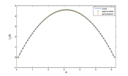
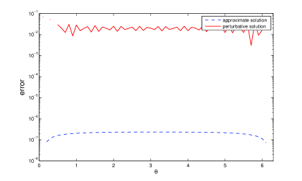
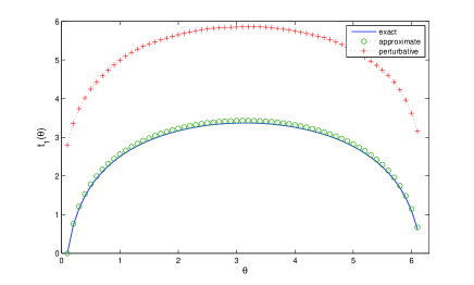
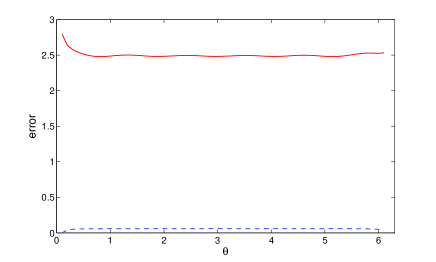
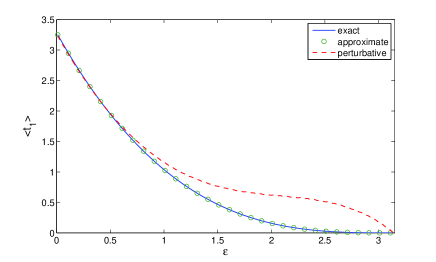
While the previous expression of t1subscript𝑡1t_{1} is exact, it is not fully explicit, since it requires either the inversion of the matrix IΩQ𝐼Ω𝑄I-\Omega Q or the calculation of all the powers of Q𝑄Q. We give here an approximation of (IΩQ)1superscript𝐼Ω𝑄1(I-\Omega Q)^{-1}, which in turn provides a convenient and fully explicit representation of t1subscript𝑡1t_{1}. As shown numerically (see Figs. 2, 3, 4 and section V for more details about numerical methods), this approximation of t1subscript𝑡1t_{1} proves to be in quantitative agreement with the exact expression for a wide range of parameters.

This approximation relies on the fact that, in the small target size limit ϵ0italic-ϵ0\epsilon\to 0, the matrix Q𝑄Q is diagonal, which mirrors the orthogonality of the {cos(nθ)}nsubscript𝑛𝜃𝑛\{\cos(n\theta)\}_{n} on [0,2π]02𝜋[0,2\pi]. More precisely, one has from Eqs. (23,24):

Qm,n=δm,nQn,n+𝒪(ϵ3),subscript𝑄𝑚𝑛subscript𝛿𝑚𝑛subscript𝑄𝑛𝑛𝒪superscriptitalic-ϵ3Q_{m,n}=\delta_{m,n}Q_{n,n}+{\cal O}(\epsilon^{3}), (30)

and keeping only the leading term of this expansion yields

dnΩ(1ΩQn,n)1Un,subscript𝑑𝑛Ωsuperscript1Ωsubscript𝑄𝑛𝑛1subscript𝑈𝑛d_{n}\approx\Omega(1-\Omega Q_{n,n})^{-1}U_{n}, (31)

from which we obtain the desired approximation:

ψ(θ)(θϵ)(2πϵθ)+4Ωn=1(cos(nθ)cos(nϵ))n(πϵ)cos(nϵ)+sin(nϵ)n31xnn2+Ω(1xn)Iϵ(n,n).𝜓𝜃𝜃italic-ϵ2𝜋italic-ϵ𝜃4Ωsuperscriptsubscript𝑛1𝑛𝜃𝑛italic-ϵ𝑛𝜋italic-ϵ𝑛italic-ϵ𝑛italic-ϵsuperscript𝑛31superscript𝑥𝑛superscript𝑛2Ω1superscript𝑥𝑛subscript𝐼italic-ϵ𝑛𝑛\psi(\theta)\approx(\theta-\epsilon)(2\pi-\epsilon-\theta)+4\Omega\sum_{n=1}^{\infty}(\cos(n\theta)-\cos(n\epsilon))\frac{n(\pi-\epsilon)\cos(n\epsilon)+\sin(n\epsilon)}{n^{3}}\frac{1-x^{n}}{n^{2}+\Omega(1-x^{n})I_{\epsilon}(n,n)}. (32)

This yields an approximation for the search time:

t1ω2T2π{23(πϵ)34Ωn=11xnn2((πϵ)cos(nϵ)+sin(nϵ)n)2n2+Ω(1xn)(πϵ+sin(2nϵ)2n)}.delimited-⟨⟩subscript𝑡1superscript𝜔2𝑇2𝜋23superscript𝜋italic-ϵ34Ωsuperscriptsubscript𝑛11superscript𝑥𝑛superscript𝑛2superscript𝜋italic-ϵ𝑛italic-ϵ𝑛italic-ϵ𝑛2superscript𝑛2Ω1superscript𝑥𝑛𝜋italic-ϵ2𝑛italic-ϵ2𝑛\langle t_{1}\rangle\approx\frac{\omega^{2}T}{2\pi}\left\{\frac{2}{3}(\pi-\epsilon)^{3}-4\Omega\sum\limits_{n=1}^{\infty}\frac{1-x^{n}}{n^{2}}~{}\frac{\bigl{(}(\pi-\epsilon)\cos(n\epsilon)+\frac{\sin(n\epsilon)}{n}\bigr{)}^{2}}{n^{2}+\Omega(1-x^{n})\bigl{(}\pi-\epsilon+\frac{\sin(2n\epsilon)}{2n}\bigr{)}}\right\}. (33)
Refer to caption
Refer to caption
Refer to caption
Refer to caption
Refer to caption
Refer to caption
Refer to caption
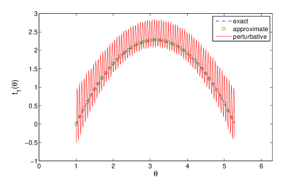
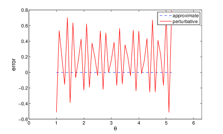
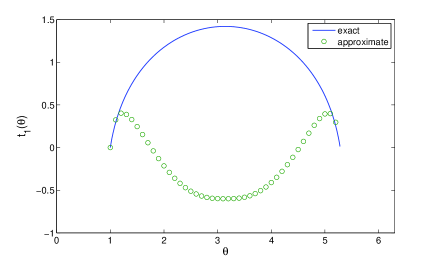
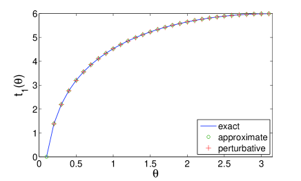
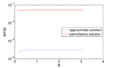
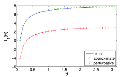
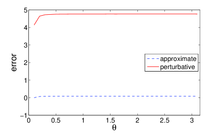
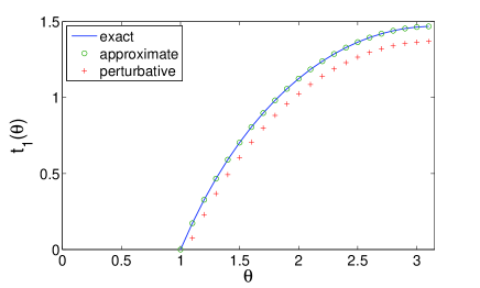
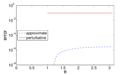
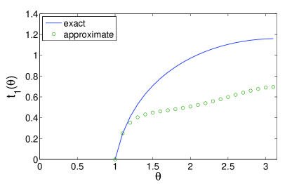
Figure 2: Comparison between three approaches for computing t1(θ)subscript𝑡1𝜃t_{1}(\theta) in 2D: the exact solution (20, 25), the approximation (32) and the perturbative formula (102), with D2=1subscript𝐷21D_{2}=1, a=0.01𝑎0.01a=0.01. In the first row, the other parameters are: ϵ=0.1italic-ϵ0.1\epsilon=0.1, λ=1𝜆1\lambda=1, and the series are truncated to N=100𝑁100N=100. On the right, the absolute error between the exact solution and the approximation (dashed blue curve) and between the exact solution and the perturbative formula (solid red curve). The approximation is very accurate indeed. In the second row, the parameters are: ϵ=0.1italic-ϵ0.1\epsilon=0.1, λ=1000𝜆1000\lambda=1000, and the series are truncated to N=100𝑁100N=100 for the exact and approximate solutions, and to N=1000𝑁1000N=1000 for the perturbative solution. One can see that the perturbative solution is inaccurate for large values of λ𝜆\lambda, while the maximal relative error of the approximate solution is below 2%percent22\%. In the third row, the parameters are: ϵ=1italic-ϵ1\epsilon=1, λ=1𝜆1\lambda=1, and the series are truncated to N=100𝑁100N=100. The perturbative solution is evidently not applicable. In the last row, the parameters are: ϵ=1italic-ϵ1\epsilon=1, λ=1000𝜆1000\lambda=1000, and the series are truncated to N=100𝑁100N=100. In this case, the approximate solution significantly deviates from the exact one (providing mostly negative values). The perturbative solution is completely invalid (not shown).
Refer to caption
Refer to caption
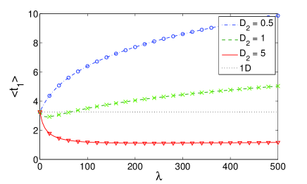
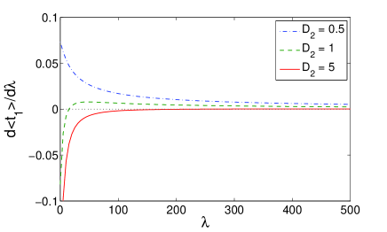
Figure 3: Left: In 2D, the mean time t1delimited-⟨⟩subscript𝑡1\langle t_{1}\rangle computed through Eq. (25, 29) with N=100𝑁100N=100 as a function of the desorption rate λ𝜆\lambda for three values of D2subscript𝐷2D_{2}: D2=0.5subscript𝐷20.5D_{2}=0.5 (dot-dashed blue line), D2=1subscript𝐷21D_{2}=1 (dashed green line), and D2=5subscript𝐷25D_{2}=5 (solid red line). The other parameters are: a=0.1𝑎0.1a=0.1 and ϵ=0.01italic-ϵ0.01\epsilon=0.01. When D2<D2,crit0.6348subscript𝐷2subscript𝐷2crit0.6348D_{2}<D_{2,\rm crit}\approx 0.6348... (the first case), t1delimited-⟨⟩subscript𝑡1\langle t_{1}\rangle monotonously increases with λ𝜆\lambda so that there is no optimal value. In two other cases, D2>D2,critsubscript𝐷2subscript𝐷2critD_{2}>D_{2,\rm crit}, and t1delimited-⟨⟩subscript𝑡1\langle t_{1}\rangle starts first to decrease with λ𝜆\lambda, passes through a minimum (the optimal value) and monotonously increases. Symbols show the approximate mean time computed through Eq. (31, 29). One can see that the approximation accurate enough even for large values of λ𝜆\lambda. Right: The derivative dt1dλ𝑑delimited-⟨⟩subscript𝑡1𝑑𝜆\frac{d\langle t_{1}\rangle}{d\lambda} defined by Eq. (35) for the same parameters.
Refer to caption
Refer to caption
Figure 4: In 2D, the mean time t1delimited-⟨⟩subscript𝑡1\langle t_{1}\rangle as a function of ϵitalic-ϵ\epsilon, with D2=1subscript𝐷21D_{2}=1, a=0.01𝑎0.01a=0.01, and λ=1𝜆1\lambda=1 (left) or λ=1000𝜆1000\lambda=1000 (right). The exact computation through Eq. (25, 29) is compared to the approximation (31, 29) and to the perturbative approach. In all cases, the series are truncated to N=100𝑁100N=100. For small λ𝜆\lambda (λ=1𝜆1\lambda=1), the approximate solution is very close to the exact one, while the perturbative solution is relatively close for ϵitalic-ϵ\epsilon up to 111. In turn, for large λ𝜆\lambda (λ=1000𝜆1000\lambda=1000), the approximate solution shows significant deviations for the intermediate values of ϵitalic-ϵ\epsilon, while the perturbative solution is not applicable at all.

III.6 Variations of the search time t1delimited-⟨⟩subscript𝑡1\langle t_{1}\rangle with the desorption rate λ𝜆\lambda

In this section, we answer two important questions. When are bulk excursions favorable, meaning enabling to reduce the search time (with respect to the situation with no bulk excursion corresponding to λ=0𝜆0\lambda=0)? If so, is there an optimal value of the desorption rate λ𝜆\lambda minimizing the search time?

III.6.1 When are bulk excursions beneficial to the search?

This question can be investigated by studying the sign of the derivative t1λdelimited-⟨⟩subscript𝑡1𝜆\frac{\partial\langle t_{1}\rangle}{\partial\lambda} at λ=0𝜆0\lambda=0. The mean search time from Eq. (29) can also be written as

t1=R42π2D12(1+λη)[2πD13R2(πϵ)3λ(ξ(I+λQ~)1U)],delimited-⟨⟩subscript𝑡1superscript𝑅42superscript𝜋2superscriptsubscript𝐷121𝜆𝜂delimited-[]2𝜋subscript𝐷13superscript𝑅2superscript𝜋italic-ϵ3𝜆𝜉superscript𝐼𝜆~𝑄1𝑈\langle t_{1}\rangle=\frac{R^{4}}{2\pi^{2}D_{1}^{2}}\bigl{(}1+\lambda\eta\bigr{)}\biggl{[}\frac{2\pi D_{1}}{3R^{2}}(\pi-\epsilon)^{3}-\lambda\bigl{(}\xi\cdot(I+\lambda\tilde{Q})^{-1}U\bigr{)}\biggr{]}, (34)

where Q~=QR2πD1~𝑄𝑄superscript𝑅2𝜋subscript𝐷1\tilde{Q}=-Q\frac{R^{2}}{\pi D_{1}}, η=2aRa24D2𝜂2𝑎𝑅superscript𝑎24subscript𝐷2\eta=\frac{2aR-a^{2}}{4D_{2}}. The derivative of t1delimited-⟨⟩subscript𝑡1\langle t_{1}\rangle with respect to λ𝜆\lambda is then

t1λ=R4η2π2D12[2πD13R2(πϵ)3(ξ(η1+2λ)I+λ2Q~(I+λQ~)2U)].delimited-⟨⟩subscript𝑡1𝜆superscript𝑅4𝜂2superscript𝜋2superscriptsubscript𝐷12delimited-[]2𝜋subscript𝐷13superscript𝑅2superscript𝜋italic-ϵ3𝜉superscript𝜂12𝜆𝐼superscript𝜆2~𝑄superscript𝐼𝜆~𝑄2𝑈\frac{\partial\langle t_{1}\rangle}{\partial\lambda}=\frac{R^{4}\eta}{2\pi^{2}D_{1}^{2}}\biggl{[}\frac{2\pi D_{1}}{3R^{2}}(\pi-\epsilon)^{3}-\biggl{(}\xi\cdot\frac{(\eta^{-1}+2\lambda)I+\lambda^{2}\tilde{Q}}{(I+\lambda\tilde{Q})^{2}}U\biggr{)}\biggr{]}. (35)

If the derivative is negative at λ=0𝜆0\lambda=0, i.e.

η2πD13R2(πϵ)3<(ξU),𝜂2𝜋subscript𝐷13superscript𝑅2superscript𝜋italic-ϵ3𝜉𝑈\eta\frac{2\pi D_{1}}{3R^{2}}(\pi-\epsilon)^{3}<\bigl{(}\xi\cdot U\bigr{)}, (36)

bulk excursions are beneficial to the search. This inequality determines the critical value for the bulk diffusion coefficient D2,critsubscript𝐷2critD_{2,\rm crit} (which enters through η𝜂\eta), above which bulk excursions are beneficial:

D1D2,crit=6R2(ξU)π(πϵ)3(2aRa2)=24π(πϵ)3(1x2)n=11xnn4[(πϵ)cos(nϵ)+sin(nϵ)n]2.subscript𝐷1subscript𝐷2crit6superscript𝑅2𝜉𝑈𝜋superscript𝜋italic-ϵ32𝑎𝑅superscript𝑎224𝜋superscript𝜋italic-ϵ31superscript𝑥2superscriptsubscript𝑛11superscript𝑥𝑛superscript𝑛4superscriptdelimited-[]𝜋italic-ϵ𝑛italic-ϵ𝑛italic-ϵ𝑛2\frac{D_{1}}{D_{2,\rm crit}}=\frac{6R^{2}(\xi\cdot U)}{\pi(\pi-\epsilon)^{3}(2aR-a^{2})}=\frac{24}{\pi(\pi-\epsilon)^{3}(1-x^{2})}\sum\limits_{n=1}^{\infty}\frac{1-x^{n}}{n^{4}}\biggl{[}(\pi-\epsilon)\cos(n\epsilon)+\frac{\sin(n\epsilon)}{n}\biggr{]}^{2}. (37)

Two comments are in order:

(i) Interestingly, this ratio depends only on a/R𝑎𝑅a/R and ϵitalic-ϵ\epsilon. In the limit of ϵ0italic-ϵ0\epsilon\to 0, one gets

D1D2,crit24π2(1x2)n=11xnn4.subscript𝐷1subscript𝐷2crit24superscript𝜋21superscript𝑥2superscriptsubscript𝑛11superscript𝑥𝑛superscript𝑛4\frac{D_{1}}{D_{2,\rm crit}}\approx\frac{24}{\pi^{2}(1-x^{2})}\sum\limits_{n=1}^{\infty}\frac{1-x^{n}}{n^{4}}. (38)

Taking next the limit a/R0𝑎𝑅0a/R\to 0 finally yields:

D1D2,crit12ζ(3)π21.4615,subscript𝐷1subscript𝐷2crit12𝜁3superscript𝜋21.4615\frac{D_{1}}{D_{2,\rm crit}}\approx\frac{12\zeta(3)}{\pi^{2}}\approx 1.4615, (39)

where ζ𝜁\zeta stands for the Riemann ζ𝜁\zeta-function.

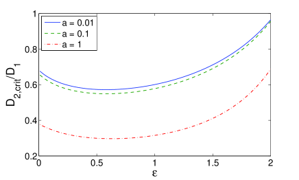
(ii) The dependence of the rhs of Eq.(37) with ϵitalic-ϵ\epsilon is not trivial (Fig. 5). Indeed it can be proved to have a maximum with respect to ϵitalic-ϵ\epsilon, which can be understood intuitively as follows: in the vicinity of ϵ=0italic-ϵ0\epsilon=0, increasing ϵitalic-ϵ\epsilon makes the constraint less stringent since the target can be reached directly from the bulk; in the opposite limit ϵπitalic-ϵ𝜋\epsilon\to\pi, the constraint on D1/D2subscript𝐷1subscript𝐷2D_{1}/D_{2} has to tend to 00 since the target is found immediately from the surface. Quantitatively, in the physical limit a0𝑎0a\to 0, one finds that, as soon as D2/D1>(D2,crit/D1)0.68subscript𝐷2subscript𝐷1subscript𝐷2critsubscript𝐷10.68D_{2}/D_{1}>(D_{2,\rm crit}/D_{1})\approx 0.68..., bulk excursions can be beneficial.

Refer to caption
Figure 5: D2,critsubscript𝐷2critD_{2,\rm crit} as a function of ϵitalic-ϵ\epsilon is computed from Eq. (37) in 2D for three values of a/R𝑎𝑅a/R: 0.010.010.01, 0.10.10.1, and 111. When ϵitalic-ϵ\epsilon approaches π𝜋\pi (the whole surface becomes absorbing), D2,critsubscript𝐷2critD_{2,\rm crit} diverges (not shown). In fact, in this limit, there is no need for a bulk excursion because the target will be found immediately by the surface diffusion.

III.6.2 When is there an optimal value of the desorption rate λ𝜆\lambda minimizing the search time?

If the reaction time t1delimited-⟨⟩subscript𝑡1\langle t_{1}\rangle is a decreasing function of the desorption rate λ𝜆\lambda, the bulk excursions are ”too favorable”, and the best search strategy is obtained for λ𝜆\lambda\to\infty (purely bulk search). For the reaction time to be an optimizable function of λ𝜆\lambda, the derivative dt1dλ𝑑delimited-⟨⟩subscript𝑡1𝑑𝜆\frac{d\langle t_{1}\rangle}{d\lambda} has to be positive at some λ𝜆\lambda. This necessary and sufficient condition remains formal and requires numerical analysis of Eq. (35). A simple sufficient condition can be used instead by demanding that the search time at zero desorption rate is less than the search time at infinite desorption rate:

t1(λ=0)<t1(λ).delimited-⟨⟩subscript𝑡1𝜆0delimited-⟨⟩subscript𝑡1𝜆\langle t_{1}(\lambda=0)\rangle<\langle t_{1}(\lambda\to\infty)\rangle. (40)

This writes in the physically relevant limit aRmuch-less-than𝑎𝑅a\ll R (using the result of Singer et al. (2006a)):

D1D2>(πϵ)33πc(ϵ),withc(ϵ)1π20πϵusin(u/2)cos(u)+cos(ϵ)du.formulae-sequencesubscript𝐷1subscript𝐷2superscript𝜋italic-ϵ33𝜋𝑐italic-ϵwith𝑐italic-ϵ1𝜋2superscriptsubscript0𝜋italic-ϵ𝑢𝑢2𝑢italic-ϵdifferential-d𝑢\displaystyle\frac{D_{1}}{D_{2}}>\frac{(\pi-\epsilon)^{3}}{3\pi c(\epsilon)},\;{\rm with}\;c(\epsilon)\equiv\frac{1}{\pi\sqrt{2}}\int_{0}^{\pi-\epsilon}\frac{u\sin(u/2)}{\sqrt{\cos(u)+\cos(\epsilon)}}{\rm d}u.

Finally, combining Eqs. (37, III.6.2), the search time is found to be an optimizable function of λ𝜆\lambda in the limit aRmuch-less-than𝑎𝑅a\ll R if

(πϵ)33πc(ϵ)<D1D2<12π(πϵ)3n=11n3[(πϵ)cos(nϵ)+sin(nϵ)n]2.superscript𝜋italic-ϵ33𝜋𝑐italic-ϵsubscript𝐷1subscript𝐷212𝜋superscript𝜋italic-ϵ3superscriptsubscript𝑛11superscript𝑛3superscriptdelimited-[]𝜋italic-ϵ𝑛italic-ϵ𝑛italic-ϵ𝑛2\frac{(\pi-\epsilon)^{3}}{3\pi c(\epsilon)}<\frac{D_{1}}{D_{2}}<\frac{12}{\pi(\pi-\epsilon)^{3}}\sum\limits_{n=1}^{\infty}\frac{1}{n^{3}}\biggl{[}(\pi-\epsilon)\cos(n\epsilon)+\frac{\sin(n\epsilon)}{n}\biggr{]}^{2}. (42)

Knowing that c(ϵ)=ln(2/ϵ)+𝒪(ϵ)𝑐italic-ϵ2italic-ϵ𝒪italic-ϵc(\epsilon)=\ln(2/\epsilon)+{\mathcal{O}}(\epsilon), Eq. (42) writes in the small ϵitalic-ϵ\epsilon limit:

π23ln(2/ϵ)<D1D2<12ζ(3)π2,superscript𝜋232italic-ϵsubscript𝐷1subscript𝐷212𝜁3superscript𝜋2\frac{\pi^{2}}{3\ln(2/\epsilon)}<\frac{D_{1}}{D_{2}}<\frac{12\zeta(3)}{\pi^{2}}, (43)

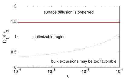
which summarizes the conditions for the search time to be an optimizable function of λ𝜆\lambda. This case is illustrated in Fig. 10.

IV 3D case

In this section, the confining domain is a sphere of radius R𝑅R and the target is the region on the boundary defined by θ[0,ϵ]𝜃0italic-ϵ\theta\in[0,\epsilon], where θ𝜃\theta is the elevation angle.

IV.1 Basic equations

The 3D analogs of Eqs. (1, 2) read as

D1R2(2t1θ2+1tanθt1θ)+λ[t2(Ra,θ)t1(θ)]subscript𝐷1superscript𝑅2superscript2subscript𝑡1superscript𝜃21𝜃subscript𝑡1𝜃𝜆delimited-[]subscript𝑡2𝑅𝑎𝜃subscript𝑡1𝜃\displaystyle\frac{D_{1}}{R^{2}}\left(\frac{\partial^{2}t_{1}}{\partial\theta^{2}}+\frac{1}{\tan\theta}\frac{\partial t_{1}}{\partial\theta}\right)+\lambda[t_{2}(R-a,\theta)-t_{1}(\theta)] =\displaystyle= 1forθ[ϵ,π],1for𝜃italic-ϵ𝜋\displaystyle-1\;\;{\rm for}\;\theta\in[\epsilon,\pi], (44)
D2(2r2+2rr+1r22θ2)t2(r,θ)subscript𝐷2superscript2superscript𝑟22𝑟𝑟1superscript𝑟2superscript2superscript𝜃2subscript𝑡2𝑟𝜃\displaystyle D_{2}\left(\frac{\partial^{2}}{\partial r^{2}}+\frac{2}{r}\frac{\partial}{\partial r}+\frac{1}{r^{2}}\frac{\partial^{2}}{\partial\theta^{2}}\right)t_{2}(r,\theta) =\displaystyle= 1.1\displaystyle-1. (45)

These equations have to be completed by two boundary conditions:

t2(R,θ)subscript𝑡2𝑅𝜃\displaystyle t_{2}(R,\theta) =\displaystyle= t1(θ),subscript𝑡1𝜃\displaystyle t_{1}(\theta), (46)
t1(θ)subscript𝑡1𝜃\displaystyle t_{1}(\theta) =\displaystyle= 0forθ[0,ϵ],0for𝜃0italic-ϵ\displaystyle 0\;\;{\rm for}\;\theta\in[0,\epsilon], (47)

which respectively describe the adsorption events and express that the target is an absorbing region of the sphere.

IV.2 Integral equation for t1subscript𝑡1t_{1}

One can search for a solution in the following form

t2(r,θ)=α0r26D2+n=1αnrnPn(cosθ),subscript𝑡2𝑟𝜃subscript𝛼0superscript𝑟26subscript𝐷2superscriptsubscript𝑛1subscript𝛼𝑛superscript𝑟𝑛subscript𝑃𝑛𝜃t_{2}(r,\theta)=\alpha_{0}-\frac{r^{2}}{6D_{2}}+\sum_{n=1}^{\infty}\alpha_{n}r^{n}P_{n}(\cos\theta), (48)

where Pnsubscript𝑃𝑛P_{n} stands for the Legendre polynomial of order n𝑛n. Using the orthonormality of Legendre polynomials, the projection of t2(R,θ)subscript𝑡2𝑅𝜃t_{2}(R,\theta) on Pmsubscript𝑃𝑚P_{m} writes

0πsinθPm(cosθ)t2(R,θ)dθ=2(α0R26D2)δm,0+2αmRm2m+1.superscriptsubscript0𝜋𝜃subscript𝑃𝑚𝜃subscript𝑡2𝑅𝜃differential-d𝜃2subscript𝛼0superscript𝑅26subscript𝐷2subscript𝛿𝑚02subscript𝛼𝑚superscript𝑅𝑚2𝑚1\int_{0}^{\pi}\sin\theta P_{m}(\cos\theta)t_{2}(R,\theta){\rm d}\theta=2\left(\alpha_{0}-\frac{R^{2}}{6D_{2}}\right)\delta_{m,0}+\frac{2\alpha_{m}R^{m}}{2m+1}. (49)

Knowing that

t2(R,θ)={t1(θ)if θ[ϵ,π],0if θ[0,ϵ],subscript𝑡2𝑅𝜃casessubscript𝑡1𝜃if θ[ϵ,π],0if θ[0,ϵ],t_{2}(R,\theta)=\begin{cases}t_{1}(\theta)&\text{if $\theta\in[\epsilon,\pi]$,}\\ 0&\text{if $\theta\in[0,\epsilon]$,}\end{cases} (50)

the αnsubscript𝛼𝑛\alpha_{n} can be written in terms of t1(θ)subscript𝑡1𝜃t_{1}(\theta) as

α0R26D2=12ϵπsinθt1(θ)dθ,αnRn=2n+12ϵπsinθPn(cosθ)t1(θ)dθifn1.formulae-sequencesubscript𝛼0superscript𝑅26subscript𝐷212superscriptsubscriptitalic-ϵ𝜋𝜃subscript𝑡1𝜃differential-d𝜃subscript𝛼𝑛superscript𝑅𝑛2𝑛12superscriptsubscriptitalic-ϵ𝜋𝜃subscript𝑃𝑛𝜃subscript𝑡1𝜃differential-d𝜃if𝑛1\begin{split}\alpha_{0}-\frac{R^{2}}{6D_{2}}&=\frac{1}{2}\int_{\epsilon}^{\pi}\sin\theta\;t_{1}(\theta){\rm d}\theta,\\ \alpha_{n}R^{n}&=\frac{2n+1}{2}\int_{\epsilon}^{\pi}\sin\theta\;P_{n}(\cos\theta)\;t_{1}(\theta){\rm d}\theta\;\;{\rm if}\;n\geq 1.\\ \end{split} (51)

Taylor expanding the rhs of

2t1θ2+1tanθt1θ=R2D1ω2[t2(Ra,θ)t2(R,θ)]superscript2subscript𝑡1superscript𝜃21𝜃subscript𝑡1𝜃superscript𝑅2subscript𝐷1superscript𝜔2delimited-[]subscript𝑡2𝑅𝑎𝜃subscript𝑡2𝑅𝜃\displaystyle\frac{\partial^{2}t_{1}}{\partial\theta^{2}}+\frac{1}{\tan\theta}\frac{\partial t_{1}}{\partial\theta}=-\frac{R^{2}}{D_{1}}-\omega^{2}[t_{2}(R-a,\theta)-t_{2}(R,\theta)] (52)

leads to

2t1θ2+1tanθt1θ=R2D1ω2k=1(a)kk!(kt2rk)R,θ.superscript2subscript𝑡1superscript𝜃21𝜃subscript𝑡1𝜃superscript𝑅2subscript𝐷1superscript𝜔2superscriptsubscript𝑘1superscript𝑎𝑘𝑘subscriptsuperscript𝑘subscript𝑡2superscript𝑟𝑘𝑅𝜃\displaystyle\frac{\partial^{2}t_{1}}{\partial\theta^{2}}+\frac{1}{\tan\theta}\frac{\partial t_{1}}{\partial\theta}=-\frac{R^{2}}{D_{1}}-\omega^{2}\sum_{k=1}^{\infty}\frac{(-a)^{k}}{k!}\left(\frac{\partial^{k}t_{2}}{\partial r^{k}}\right)_{R,\theta}. (53)

Using Eq. (48) for t2subscript𝑡2t_{2} yields

2t1θ2+1tanθt1θ=R2D1ω2(aR3D2a26D2)ω2k=1(a)kk!n=kαnn(n1)(nk+1)RnkPn(cosθ).superscript2subscript𝑡1superscript𝜃21𝜃subscript𝑡1𝜃superscript𝑅2subscript𝐷1superscript𝜔2𝑎𝑅3subscript𝐷2superscript𝑎26subscript𝐷2superscript𝜔2superscriptsubscript𝑘1superscript𝑎𝑘𝑘superscriptsubscript𝑛𝑘subscript𝛼𝑛𝑛𝑛1𝑛𝑘1superscript𝑅𝑛𝑘subscript𝑃𝑛𝜃\displaystyle\frac{\partial^{2}t_{1}}{\partial\theta^{2}}+\frac{1}{\tan\theta}\frac{\partial t_{1}}{\partial\theta}=-\frac{R^{2}}{D_{1}}-\omega^{2}\left(\frac{aR}{3D_{2}}-\frac{a^{2}}{6D_{2}}\right)-\omega^{2}\sum_{k=1}^{\infty}\frac{(-a)^{k}}{k!}\sum_{n=k}^{\infty}\alpha_{n}n(n-1)\dots(n-k+1)R^{n-k}P_{n}(\cos\theta). (54)

Changing the order of summations over n𝑛n and k𝑘k and using the binomial formula and Eq. (51) for αnsubscript𝛼𝑛\alpha_{n} finally give

2t1θ2+1tanθt1θ=R2D1ω2(aR3D2a26D2)ω22n=1(xn1)Pn(cosθ)(2n+1)ϵπsinθPn(cosθ)t1(θ)dθ,superscript2subscript𝑡1superscript𝜃21𝜃subscript𝑡1𝜃superscript𝑅2subscript𝐷1superscript𝜔2𝑎𝑅3subscript𝐷2superscript𝑎26subscript𝐷2superscript𝜔22superscriptsubscript𝑛1superscript𝑥𝑛1subscript𝑃𝑛𝜃2𝑛1superscriptsubscriptitalic-ϵ𝜋superscript𝜃subscript𝑃𝑛superscript𝜃subscript𝑡1superscript𝜃differential-dsuperscript𝜃\displaystyle\frac{\partial^{2}t_{1}}{\partial\theta^{2}}+\frac{1}{\tan\theta}\frac{\partial t_{1}}{\partial\theta}=-\frac{R^{2}}{D_{1}}-\omega^{2}\left(\frac{aR}{3D_{2}}-\frac{a^{2}}{6D_{2}}\right)-\frac{\omega^{2}}{2}\sum_{n=1}^{\infty}(x^{n}-1)P_{n}(\cos\theta)(2n+1)\int_{\epsilon}^{\pi}\sin\theta^{\prime}P_{n}(\cos\theta^{\prime})t_{1}(\theta^{\prime}){\rm d}\theta^{\prime}, (55)

where, as in previous section, x1aR𝑥1𝑎𝑅x\equiv 1-\frac{a}{R}. This integro-differential equation for t1subscript𝑡1t_{1} can actually easily be transformed into an integral equation for t1subscript𝑡1t_{1}, by integrating successively two times. Indeed, multiplying first both members of Eq. (55) by sinθ𝜃\sin\theta and integrating between π𝜋\pi and θ𝜃\theta gives

sinθt1(θ)𝜃subscriptsuperscript𝑡1𝜃\displaystyle\sin\theta~{}t^{\prime}_{1}(\theta) =\displaystyle= [R2D1+ω2(aR3D2a26D2)](cosθ+1)delimited-[]superscript𝑅2subscript𝐷1superscript𝜔2𝑎𝑅3subscript𝐷2superscript𝑎26subscript𝐷2𝜃1\displaystyle\left[\frac{R^{2}}{D_{1}}+\omega^{2}\left(\frac{aR}{3D_{2}}-\frac{a^{2}}{6D_{2}}\right)\right](\cos\theta+1) (56)
+\displaystyle+ ω22n=1(xn1)(Pn+1(cosθ)Pn1(cosθ))ϵπsinθPn(cosθ)t1(θ)dθ,superscript𝜔22superscriptsubscript𝑛1superscript𝑥𝑛1subscript𝑃𝑛1𝜃subscript𝑃𝑛1𝜃superscriptsubscriptitalic-ϵ𝜋superscript𝜃subscript𝑃𝑛superscript𝜃subscript𝑡1superscript𝜃differential-dsuperscript𝜃\displaystyle\frac{\omega^{2}}{2}\sum_{n=1}^{\infty}(x^{n}-1)\left(P_{n+1}(\cos\theta)-P_{n-1}(\cos\theta)\right)\int_{\epsilon}^{\pi}\sin\theta^{\prime}P_{n}(\cos\theta^{\prime})t_{1}(\theta^{\prime}){\rm d}\theta^{\prime},

where we have used

Pn(x)dx=1n(n+1)(1x2)Pn(x)=12n+1(Pn+1(x)Pn1(x)).subscript𝑃𝑛𝑥differential-d𝑥1𝑛𝑛11superscript𝑥2subscriptsuperscript𝑃𝑛𝑥12𝑛1subscript𝑃𝑛1𝑥subscript𝑃𝑛1𝑥\int P_{n}(x){\rm d}x=-\frac{1}{n(n+1)}(1-x^{2})P^{\prime}_{n}(x)=\frac{1}{2n+1}(P_{n+1}(x)-P_{n-1}(x)). (57)

Dividing Eq. (56) by sinθ𝜃\sin\theta and integrating between ϵitalic-ϵ\epsilon and θ𝜃\theta finally leads to

t1(θ)subscript𝑡1𝜃\displaystyle t_{1}(\theta) =\displaystyle= 2(R2D1+ω2(aR3D2a26D2))ln(sin(θ/2)sin(ϵ/2))2superscript𝑅2subscript𝐷1superscript𝜔2𝑎𝑅3subscript𝐷2superscript𝑎26subscript𝐷2𝜃2italic-ϵ2\displaystyle 2\left(\frac{R^{2}}{D_{1}}+\omega^{2}\left(\frac{aR}{3D_{2}}-\frac{a^{2}}{6D_{2}}\right)\right)\ln\left(\frac{\sin(\theta/2)}{\sin(\epsilon/2)}\right)
+\displaystyle+ ω22n=1(xn1)2n+1n(n+1)(Pn(cosθ)Pn(cosϵ))ϵπsinθPn(cosθ)t1(θ)dθ,superscript𝜔22superscriptsubscript𝑛1superscript𝑥𝑛12𝑛1𝑛𝑛1subscript𝑃𝑛𝜃subscript𝑃𝑛italic-ϵsuperscriptsubscriptitalic-ϵ𝜋superscript𝜃subscript𝑃𝑛superscript𝜃subscript𝑡1superscript𝜃differential-dsuperscript𝜃\displaystyle\frac{\omega^{2}}{2}\sum_{n=1}^{\infty}(x^{n}-1)\frac{2n+1}{n(n+1)}\left(P_{n}(\cos\theta)-P_{n}(\cos\epsilon)\right)\int_{\epsilon}^{\pi}\sin\theta^{\prime}P_{n}(\cos\theta^{\prime})t_{1}(\theta^{\prime}){\rm d}\theta^{\prime},

where we have again used Eq. (57), or equivalently to

ψ(θ)=ln(1cosθ1cosϵ)+Ωn=1(xn1)2n+1n(n+1)(Pn(cosθ)Pn(cosϵ))ϵπsin(θ)Pn(cosθ)ψ(θ)dθ,𝜓𝜃1𝜃1italic-ϵΩsuperscriptsubscript𝑛1superscript𝑥𝑛12𝑛1𝑛𝑛1subscript𝑃𝑛𝜃subscript𝑃𝑛italic-ϵsuperscriptsubscriptitalic-ϵ𝜋superscript𝜃subscript𝑃𝑛superscript𝜃𝜓superscript𝜃differential-dsuperscript𝜃\displaystyle\psi(\theta)=\ln\left(\frac{1-\cos\theta}{1-\cos\epsilon}\right)+\Omega\sum_{n=1}^{\infty}(x^{n}-1)\frac{2n+1}{n(n+1)}(P_{n}(\cos\theta)-P_{n}(\cos\epsilon))\int_{\epsilon}^{\pi}\sin(\theta^{\prime})P_{n}(\cos\theta^{\prime})\psi(\theta^{\prime}){\rm d}\theta^{\prime}, (58)

with the following definitions

ψ(θ)t1(θ)ω2T,T1λ+R2(Ra)26D2,Ωω22formulae-sequence𝜓𝜃subscript𝑡1𝜃superscript𝜔2𝑇formulae-sequence𝑇1𝜆superscript𝑅2superscript𝑅𝑎26subscript𝐷2Ωsuperscript𝜔22\psi(\theta)\equiv\frac{t_{1}(\theta)}{\omega^{2}T},\hskip 14.22636ptT\equiv\frac{1}{\lambda}+\frac{R^{2}-(R-a)^{2}}{6D_{2}},\hskip 14.22636pt\Omega\equiv\frac{\omega^{2}}{2} (59)

in this 3D case.

IV.3 Exact solution

Iterating the integral equation Eq. (58) shows that the solution ψ(θ)𝜓𝜃\psi(\theta) writes for θ[ϵ,π]𝜃italic-ϵ𝜋\theta\in[\epsilon,\pi]:

ψ(θ)=ln(1cosθ1cosϵ)+n=1dn[Pn(cosθ)Pn(cosϵ)],𝜓𝜃1𝜃1italic-ϵsuperscriptsubscript𝑛1subscript𝑑𝑛delimited-[]subscript𝑃𝑛𝜃subscript𝑃𝑛italic-ϵ\psi(\theta)=\ln\left(\frac{1-\cos\theta}{1-\cos\epsilon}\right)+\sum\limits_{n=1}^{\infty}d_{n}\bigl{[}P_{n}(\cos\theta)-P_{n}(\cos\epsilon)\bigr{]}, (60)

with the coefficients dnsubscript𝑑𝑛d_{n} which satisfy

n=1dn[Pn(cosθ)Pn(cosϵ)]=Ωn=1(Un+n=1Qn,ndn)[Pn(cosθ)Pn(cosϵ)],superscriptsubscript𝑛1subscript𝑑𝑛delimited-[]subscript𝑃𝑛𝜃subscript𝑃𝑛italic-ϵΩsuperscriptsubscript𝑛1subscript𝑈𝑛superscriptsubscriptsuperscript𝑛1subscript𝑄𝑛superscript𝑛subscript𝑑superscript𝑛delimited-[]subscript𝑃𝑛𝜃subscript𝑃𝑛italic-ϵ\begin{split}&\sum\limits_{n=1}^{\infty}d_{n}\bigl{[}P_{n}(\cos\theta)-P_{n}(\cos\epsilon)\bigr{]}=\Omega\sum\limits_{n=1}^{\infty}\biggl{(}U_{n}+\sum\limits_{n^{\prime}=1}^{\infty}Q_{n,n^{\prime}}d_{n^{\prime}}\biggr{)}\bigl{[}P_{n}(\cos\theta)-P_{n}(\cos\epsilon)\bigr{]},\\ \end{split} (61)

where we introduced the new definitions

Un(xn1)(2n+1)n(n+1)ϵπdθsin(θ)Pn(cosθ)ln(1cosθ1cosϵ)=(1xn)(2n+1)n2(n+1)2ξn,ξn(1+ncosϵn+1)Pn(cosϵ)+Pn1(cosϵ)n+1(n=1,2,),formulae-sequencesubscript𝑈𝑛superscript𝑥𝑛12𝑛1𝑛𝑛1superscriptsubscriptitalic-ϵ𝜋differential-dsuperscript𝜃superscript𝜃subscript𝑃𝑛superscript𝜃1superscript𝜃1italic-ϵ1superscript𝑥𝑛2𝑛1superscript𝑛2superscript𝑛12subscript𝜉𝑛subscript𝜉𝑛1𝑛italic-ϵ𝑛1subscript𝑃𝑛italic-ϵsubscript𝑃𝑛1italic-ϵ𝑛1𝑛12\begin{split}U_{n}&\equiv\frac{(x^{n}-1)(2n+1)}{n(n+1)}\int\limits_{\epsilon}^{\pi}{\rm d}\theta^{\prime}\sin(\theta^{\prime})P_{n}(\cos\theta^{\prime})\ln\left(\frac{1-\cos\theta^{\prime}}{1-\cos\epsilon}\right)=\frac{(1-x^{n})(2n+1)}{n^{2}(n+1)^{2}}~{}\xi_{n},\\ \xi_{n}&\equiv\biggl{(}1+\frac{n\cos\epsilon}{n+1}\biggr{)}P_{n}(\cos\epsilon)+\frac{P_{n-1}(\cos\epsilon)}{n+1}\hskip 14.22636pt(n=1,2,...),\\ \end{split} (62)

and

Qn,n(1xn)(2n+1)n(n+1)Iϵ(n,n)(n,n=1,2,),Q_{n,n^{\prime}}\equiv-\frac{(1-x^{n})(2n+1)}{n(n+1)}I_{\epsilon}(n,n^{\prime})\hskip 14.22636pt(n,n^{\prime}=1,2,...), (63)

with

Iϵ(n,n)1cosϵPn(u)(Pn(u)Pn(cosϵ))du.subscript𝐼italic-ϵ𝑛superscript𝑛superscriptsubscript1italic-ϵsubscript𝑃𝑛𝑢subscript𝑃superscript𝑛𝑢subscript𝑃superscript𝑛italic-ϵdifferential-d𝑢I_{\epsilon}(n,n^{\prime})\equiv\int\limits_{-1}^{\cos\epsilon}P_{n}(u)(P_{n^{\prime}}(u)-P_{n^{\prime}}(\cos\epsilon)){\rm d}u. (64)

In Appendix C, we compute this integral explicitly.

Since Eq. (58) should be satisfied for any θ𝜃\theta, one gets 𝐝=Ω(U+Q𝐝)𝐝Ω𝑈𝑄𝐝{\bf d}=\Omega(U+Q{\bf d}), from which

dn=Ω[(IΩQ)1U]n(n=1,2,).subscript𝑑𝑛Ωsubscriptdelimited-[]superscript𝐼Ω𝑄1𝑈𝑛𝑛12d_{n}=\Omega\bigl{[}(I-\Omega Q)^{-1}U\bigr{]}_{n}\hskip 14.22636pt(n=1,2,...). (65)

As in 2D, using the series expansion of (IΩQ)1superscript𝐼Ω𝑄1(I-\Omega Q)^{-1}, Eq. (65) can be seen as a series in powers of ΩΩ\Omega, whose n𝑛n-th order coefficient can be explicitly written in terms of the n𝑛n-th power of the matrix Q𝑄Q.

Note that the first term in Eq. (60) can also be represented as a series

n=1en[Pn(cosθ)Pn(cosϵ)]={ln(1cosθ1cosϵ),ϵ<θ<πϵ0,otherwise,superscriptsubscript𝑛1subscript𝑒𝑛delimited-[]subscript𝑃𝑛𝜃subscript𝑃𝑛italic-ϵcases1𝜃1italic-ϵitalic-ϵ𝜃𝜋italic-ϵotherwise0otherwiseotherwise\sum\limits_{n=1}^{\infty}e_{n}\bigl{[}P_{n}(\cos\theta)-P_{n}(\cos\epsilon)\bigr{]}=\begin{cases}\ln\left(\frac{1-\cos\theta}{1-\cos\epsilon}\right),~{}~{}~{}\epsilon<\theta<\pi-\epsilon\cr~{}\hskip 22.76219pt0,\hskip 36.98857pt{\rm otherwise},\end{cases} (66)

where the coefficients ensubscript𝑒𝑛e_{n} are obtained by multiplying this equation by Pn(cosθ)sinθsubscript𝑃𝑛𝜃𝜃P_{n}(\cos\theta)\sin\theta and integrating from 00 to π𝜋\pi:

en=2n+12n(n+1)ξn.subscript𝑒𝑛2𝑛12𝑛𝑛1subscript𝜉𝑛e_{n}=-\frac{2n+1}{2n(n+1)}\xi_{n}. (67)

Once the dnsubscript𝑑𝑛d_{n} determined, the search time t1delimited-⟨⟩subscript𝑡1\langle t_{1}\rangle can be written as

t1ω2T2ϵπ𝑑θsinθψ(θ)=ω2T2{2ln(21cosϵ)(1+cosϵ)n=1dnξn}.delimited-⟨⟩subscript𝑡1superscript𝜔2𝑇2superscriptsubscriptitalic-ϵ𝜋differential-d𝜃𝜃𝜓𝜃superscript𝜔2𝑇2221italic-ϵ1italic-ϵsuperscriptsubscript𝑛1subscript𝑑𝑛subscript𝜉𝑛\begin{split}\langle t_{1}\rangle&\equiv\frac{\omega^{2}T}{2}\int\limits_{\epsilon}^{\pi}d\theta~{}\sin\theta~{}\psi(\theta)=\frac{\omega^{2}T}{2}\biggl{\{}2\ln\left(\frac{2}{1-\cos\epsilon}\right)-(1+\cos\epsilon)-\sum\limits_{n=1}^{\infty}d_{n}\xi_{n}\biggr{\}}.\\ \end{split} (68)

IV.4 Perturbative solution

The first terms of a perturbative expansion with respect to ϵitalic-ϵ\epsilon can easily be obtained from the previous exact solution. At leading order in ϵitalic-ϵ\epsilon, we have

Un=Un(0)+O(ϵ)=2(1xn)(2n+1)n2(n+1)2+O(ϵ),Qm,n=Qm,n(0)+O(ϵ)=2(1xn)n(n+1)δm,n+O(ϵ),formulae-sequencesubscript𝑈𝑛superscriptsubscript𝑈𝑛0𝑂italic-ϵ21superscript𝑥𝑛2𝑛1superscript𝑛2superscript𝑛12𝑂italic-ϵsubscript𝑄𝑚𝑛superscriptsubscript𝑄𝑚𝑛0𝑂italic-ϵ21superscript𝑥𝑛𝑛𝑛1subscript𝛿𝑚𝑛𝑂italic-ϵ\begin{split}U_{n}&=U_{n}^{(0)}+O(\epsilon)=\frac{2(1-x^{n})(2n+1)}{n^{2}(n+1)^{2}}+O(\epsilon),\\ Q_{m,n}&=Q_{m,n}^{(0)}+O(\epsilon)=-\frac{2(1-x^{n})}{n(n+1)}\delta_{m,n}+O(\epsilon),\\ \end{split} (69)

from which

dn=Ω[(IΩQ(0))1U(0)]n+O(ϵ)=2Ωn(n+1)(1xn)(2n+1)n(n+1)+2Ω(1xn)+O(ϵ).subscript𝑑𝑛Ωsubscriptdelimited-[]superscript𝐼Ωsuperscript𝑄01superscript𝑈0𝑛𝑂italic-ϵ2Ω𝑛𝑛11superscript𝑥𝑛2𝑛1𝑛𝑛12Ω1superscript𝑥𝑛𝑂italic-ϵd_{n}=\Omega\bigl{[}(I-\Omega Q^{(0)})^{-1}U^{(0)}\bigr{]}_{n}+O(\epsilon)=\frac{2\Omega}{n(n+1)}~{}\frac{(1-x^{n})(2n+1)}{n(n+1)+2\Omega(1-x^{n})}+O(\epsilon). (70)

One finds therefore

ψ(θ)=2lnϵ+2ln(2sin(θ/2))2Ωn=1(1xn)2n+1n(n+1)1Pn(cosθ)n(n+1)+2Ω(1xn)+O(ϵ).𝜓𝜃2italic-ϵ22𝜃22Ωsuperscriptsubscript𝑛11superscript𝑥𝑛2𝑛1𝑛𝑛11subscript𝑃𝑛𝜃𝑛𝑛12Ω1superscript𝑥𝑛𝑂italic-ϵ\psi(\theta)=-2\ln\epsilon+2\ln\left(2\sin(\theta/2)\right)-2\Omega\sum_{n=1}^{\infty}(1-x^{n})\frac{2n+1}{n(n+1)}~{}\frac{1-P_{n}(\cos\theta)}{n(n+1)+2\Omega(1-x^{n})}+O(\epsilon). (71)

Averaging over θ𝜃\theta, it finally yields:

t1ω2T{2ln(ϵ/2)12Ωn=12n+1n(n+1)(1xn)n(n+1)+2Ω(1xn)+O(ϵ)}.delimited-⟨⟩subscript𝑡1superscript𝜔2𝑇2italic-ϵ212Ωsuperscriptsubscript𝑛12𝑛1𝑛𝑛11superscript𝑥𝑛𝑛𝑛12Ω1superscript𝑥𝑛𝑂italic-ϵ\langle t_{1}\rangle\approx\omega^{2}T\biggl{\{}-2\ln(\epsilon/2)-1-2\Omega\sum_{n=1}^{\infty}\frac{2n+1}{n(n+1)}~{}\frac{(1-x^{n})}{n(n+1)+2\Omega(1-x^{n})}+O(\epsilon)\biggr{\}}. (72)

This result was given in Bénichou et al. (2010) without derivation.

IV.5 Approximate solution

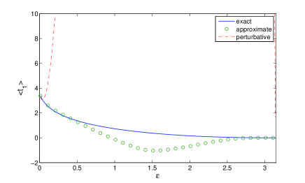
As earlier for the 2D case, an approximate solution can be derived. As shown numerically (see Figs. 6, 7, 8 and section V for more details about numerical methods), this approximation of t1subscript𝑡1t_{1} proves to be in quantitative agreement with the exact expression for a wide range of parameters.

This approximation relies on the fact that, in the small target size limit ϵ0italic-ϵ0\epsilon\to 0, the matrix Q𝑄Q is diagonal, which in turn mirrors the orthogonality of {Pn(cosθ)}nsubscriptsubscript𝑃𝑛𝜃𝑛\{P_{n}(\cos\theta)\}_{n} on [0,π]0𝜋[0,\pi]. More precisely, one has

Qm,n=δm,nQn,n+𝒪(ϵ4),subscript𝑄𝑚𝑛subscript𝛿𝑚𝑛subscript𝑄𝑛𝑛𝒪superscriptitalic-ϵ4Q_{m,n}=\delta_{m,n}Q_{n,n}+{\cal O}(\epsilon^{4}), (73)

and keeping only the leading term of this expansion yields

dnΩ(1ΩQn,n)1Un,subscript𝑑𝑛Ωsuperscript1Ωsubscript𝑄𝑛𝑛1subscript𝑈𝑛d_{n}\approx\Omega(1-\Omega Q_{n,n})^{-1}U_{n}, (74)

from which

ψ(θ)ln(1cosθ1cosϵ)+Ωn=1(1xn)2n+1n(n+1)(Pn(cosθ)Pn(cosϵ))(1+ncosϵn+1)Pn(cosϵ)+Pn1(cosϵ)n+1n(n+1)+Ω(1xn)(2n+1)Iϵ(n,n).𝜓𝜃1𝜃1italic-ϵΩsuperscriptsubscript𝑛11superscript𝑥𝑛2𝑛1𝑛𝑛1subscript𝑃𝑛𝜃subscript𝑃𝑛italic-ϵ1𝑛italic-ϵ𝑛1subscript𝑃𝑛italic-ϵsubscript𝑃𝑛1italic-ϵ𝑛1𝑛𝑛1Ω1superscript𝑥𝑛2𝑛1subscript𝐼italic-ϵ𝑛𝑛\psi(\theta)\approx\ln\left(\frac{1-\cos\theta}{1-\cos\epsilon}\right)+\Omega\sum_{n=1}^{\infty}(1-x^{n})\frac{2n+1}{n(n+1)}(P_{n}(\cos\theta)-P_{n}(\cos\epsilon))\frac{\bigl{(}1+\frac{n\cos\epsilon}{n+1}\bigr{)}P_{n}(\cos\epsilon)+\frac{P_{n-1}(\cos\epsilon)}{n+1}}{n(n+1)+\Omega(1-x^{n})(2n+1)I_{\epsilon}(n,n)}. (75)

The mean time t1delimited-⟨⟩subscript𝑡1\langle t_{1}\rangle is then approximated as

t1ω2T{ln(21cosϵ)1+cosϵ2Ω2n=1(1xn)(2n+1)n(n+1)[(1+ncosϵn+1)Pn(cosϵ)+Pn1(cosϵ)n+1]2n(n+1)+Ω(1xn)(2n+1)Iϵ(n,n)]}.\begin{split}\langle t_{1}\rangle&\approx\omega^{2}T\biggl{\{}\ln\left(\frac{2}{1-\cos\epsilon}\right)-\frac{1+\cos\epsilon}{2}\\ &-\frac{\Omega}{2}\sum\limits_{n=1}^{\infty}\frac{(1-x^{n})(2n+1)}{n(n+1)}\frac{\bigl{[}\bigl{(}1+\frac{n\cos\epsilon}{n+1}\bigr{)}P_{n}(\cos\epsilon)+\frac{P_{n-1}(\cos\epsilon)}{n+1}\bigr{]}^{2}}{n(n+1)+\Omega(1-x^{n})(2n+1)I_{\epsilon}(n,n)}\biggr{]}\biggr{\}}.\\ \end{split} (76)
Refer to caption
Refer to caption
Refer to caption
Refer to caption
Refer to caption
Refer to caption
Refer to caption
Figure 6: Comparison between three approaches for computing t1(θ)subscript𝑡1𝜃t_{1}(\theta) in 3D: the exact solution (60, 65), the approximation (75) and the perturbative formula (71), with D2=1subscript𝐷21D_{2}=1, a=0.01𝑎0.01a=0.01. In the first row, the other parameters are: ϵ=0.1italic-ϵ0.1\epsilon=0.1, λ=1𝜆1\lambda=1, and the series are truncated to N=100𝑁100N=100. On the right, the absolute error between the exact solution and the approximation (dashed blue curve) and between the exact solution and the perturbative formula (solid red curve). The approximation is very accurate indeed. In the second row, the parameters are: ϵ=0.1italic-ϵ0.1\epsilon=0.1, λ=1000𝜆1000\lambda=1000, and the series are truncated to N=100𝑁100N=100. One can see that the perturbative solution is inaccurate for large values of λ𝜆\lambda, while the maximal relative error of the approximate solution is still small. In the third row, the parameters are: ϵ=1italic-ϵ1\epsilon=1, λ=1𝜆1\lambda=1, and the series are truncated to N=100𝑁100N=100. The perturbative solution is inaccurate as expected for large ϵitalic-ϵ\epsilon. In the last row, the parameters are: ϵ=1italic-ϵ1\epsilon=1, λ=1000𝜆1000\lambda=1000, and the series are truncated to N=100𝑁100N=100. In this case, the approximate solution deviates from the exact one for. The perturbative solution is negative and not shown.
Refer to caption
Refer to caption
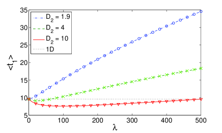
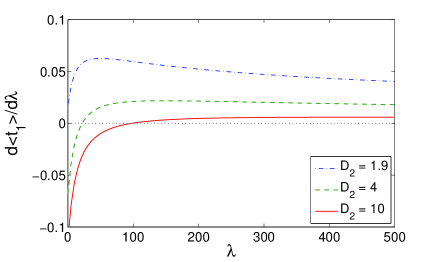
Figure 7: Left: In 3D, the mean time t1delimited-⟨⟩subscript𝑡1\langle t_{1}\rangle computed through Eq. (65, 68) with N=100𝑁100N=100 as a function of the desorption rate λ𝜆\lambda for three values of D2subscript𝐷2D_{2}: D2=1.9subscript𝐷21.9D_{2}=1.9 (dot-dashed blue line), D2=4subscript𝐷24D_{2}=4 (dashed green line), and D2=10subscript𝐷210D_{2}=10 (solid red line). The other parameters are: a=0.1𝑎0.1a=0.1 and ϵ=0.01italic-ϵ0.01\epsilon=0.01. When D2<D2,crit1.9997.subscript𝐷2subscript𝐷2crit1.9997D_{2}<D_{2,\rm crit}\approx 1.9997.... (the first case), t1delimited-⟨⟩subscript𝑡1\langle t_{1}\rangle monotonously increases with λ𝜆\lambda so that there is no optimal value. In two other cases, D2>D2,critsubscript𝐷2subscript𝐷2critD_{2}>D_{2,\rm crit}, and t1delimited-⟨⟩subscript𝑡1\langle t_{1}\rangle starts first to decrease with λ𝜆\lambda, passes through a minimum (the optimal value) and then increases. Symbols show the approximate mean time computed through Eq. (76). One can see that the approximation accurate enough even for large values of λ𝜆\lambda. Right: The derivative dt1dλ𝑑delimited-⟨⟩subscript𝑡1𝑑𝜆\frac{d\langle t_{1}\rangle}{d\lambda} defined by Eq. (78) for the same parameters.
Refer to caption
Refer to caption
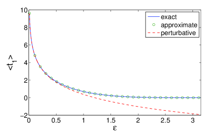
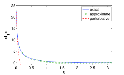
Figure 8: In 3D, the mean time t1delimited-⟨⟩subscript𝑡1\langle t_{1}\rangle as a function of ϵitalic-ϵ\epsilon, with D2=1subscript𝐷21D_{2}=1, a=0.01𝑎0.01a=0.01, and λ=1𝜆1\lambda=1 (left) or λ=1000𝜆1000\lambda=1000 (right). The exact computation through Eq. (65, 68) is compared to the approximation (76) and to the perturbative approach. In all cases, the series are truncated to N=100𝑁100N=100. For small λ𝜆\lambda (λ=1𝜆1\lambda=1), the approximate solution is very close to the exact one, while the perturbative solution is relatively close for ϵitalic-ϵ\epsilon up to 111. In turn, for large λ𝜆\lambda (λ=1000𝜆1000\lambda=1000), the approximate solution shows significant deviations for the intermediate values of ϵitalic-ϵ\epsilon, while the perturbative solution is not applicable at all.

IV.6 Variations of the search time t1delimited-⟨⟩subscript𝑡1\langle t_{1}\rangle with the desorption rate λ𝜆\lambda

We investigate here as in the 2D case the dependence of t1delimited-⟨⟩subscript𝑡1\langle t_{1}\rangle on λ𝜆\lambda.

IV.6.1 When are bulk excursions beneficial to the search?

The sign of t1λdelimited-⟨⟩subscript𝑡1𝜆\frac{\partial\langle t_{1}\rangle}{\partial\lambda} at λ=0𝜆0\lambda=0 is conveniently studied by rewriting Eq. (68) as

t1=R44D12(1+λη){4D1R2[ln(21cosϵ)1+cosϵ2]λ(ξ(I+λQ~)1U)},delimited-⟨⟩subscript𝑡1superscript𝑅44superscriptsubscript𝐷121𝜆𝜂4subscript𝐷1superscript𝑅2delimited-[]21italic-ϵ1italic-ϵ2𝜆𝜉superscript𝐼𝜆~𝑄1𝑈\langle t_{1}\rangle=\frac{R^{4}}{4D_{1}^{2}}\bigl{(}1+\lambda\eta\bigr{)}\biggl{\{}\frac{4D_{1}}{R^{2}}\biggl{[}\ln\left(\frac{2}{1-\cos\epsilon}\right)-\frac{1+\cos\epsilon}{2}\biggr{]}-\lambda\bigl{(}\xi\cdot(I+\lambda\tilde{Q})^{-1}U\bigr{)}\biggr{\}}, (77)

where Q~=QR22D1~𝑄𝑄superscript𝑅22subscript𝐷1\tilde{Q}=-Q\frac{R^{2}}{2D_{1}} and η=2aRa26D2𝜂2𝑎𝑅superscript𝑎26subscript𝐷2\eta=\frac{2aR-a^{2}}{6D_{2}}. The derivative of t1delimited-⟨⟩subscript𝑡1\langle t_{1}\rangle with respect to λ𝜆\lambda is then

t1λ=R4η4D12{[ln(21cosϵ)1+cosϵ2](ξ(η1+2λ)I+λ2Q~(I+λQ~)2U)}.delimited-⟨⟩subscript𝑡1𝜆superscript𝑅4𝜂4superscriptsubscript𝐷12delimited-[]21italic-ϵ1italic-ϵ2𝜉superscript𝜂12𝜆𝐼superscript𝜆2~𝑄superscript𝐼𝜆~𝑄2𝑈\frac{\partial\langle t_{1}\rangle}{\partial\lambda}=\frac{R^{4}\eta}{4D_{1}^{2}}\biggl{\{}\biggl{[}\ln\left(\frac{2}{1-\cos\epsilon}\right)-\frac{1+\cos\epsilon}{2}\biggr{]}-\biggl{(}\xi\cdot\frac{(\eta^{-1}+2\lambda)I+\lambda^{2}\tilde{Q}}{(I+\lambda\tilde{Q})^{2}}U\biggr{)}\biggr{\}}. (78)

If the above derivative is negative at λ=0𝜆0\lambda=0, i.e.

4D1R2(ln(21cosϵ)1+cosϵ2)<(ξU)η,4subscript𝐷1superscript𝑅221italic-ϵ1italic-ϵ2𝜉𝑈𝜂\frac{4D_{1}}{R^{2}}~{}\biggl{(}\ln\left(\frac{2}{1-\cos\epsilon}\right)-\frac{1+\cos\epsilon}{2}\biggr{)}<\frac{(\xi\cdot U)}{\eta}, (79)

bulk excursions are beneficial to the search. This inequality determines the critical value for the bulk diffusion coefficient D2,critsubscript𝐷2critD_{2,\rm crit} (which enters through η𝜂\eta):

D2,critD1=(ln(21cosϵ)1+cosϵ2)2(2aRa2)3R2(ξU)=(ln(21cosϵ)1+cosϵ2)2(1x2)3×(n=1(1xn)(2n+1)n2(n+1)4[(n+1+ncosϵ)Pn(cosϵ)+Pn1(cosϵ)]2)1.subscript𝐷2critsubscript𝐷121italic-ϵ1italic-ϵ222𝑎𝑅superscript𝑎23superscript𝑅2𝜉𝑈21italic-ϵ1italic-ϵ221superscript𝑥23superscriptsuperscriptsubscript𝑛11superscript𝑥𝑛2𝑛1superscript𝑛2superscript𝑛14superscriptdelimited-[]𝑛1𝑛italic-ϵsubscript𝑃𝑛italic-ϵsubscript𝑃𝑛1italic-ϵ21\begin{split}\frac{D_{2,\rm crit}}{D_{1}}&=\biggl{(}\ln\left(\frac{2}{1-\cos\epsilon}\right)-\frac{1+\cos\epsilon}{2}\biggr{)}\frac{2(2aR-a^{2})}{3R^{2}(\xi\cdot U)}\\ &=\biggl{(}\ln\left(\frac{2}{1-\cos\epsilon}\right)-\frac{1+\cos\epsilon}{2}\biggr{)}\frac{2(1-x^{2})}{3}\\ &\times\biggl{(}\sum\limits_{n=1}^{\infty}\frac{(1-x^{n})(2n+1)}{n^{2}(n+1)^{4}}\bigl{[}(n+1+n\cos\epsilon)P_{n}(\cos\epsilon)+P_{n-1}(\cos\epsilon)\bigr{]}^{2}\biggr{)}^{-1}.\\ \end{split} (80)

In the limit of ϵ0italic-ϵ0\epsilon\to 0, one gets

D2,critD1(2ln(2/ϵ)1)(1x2)6(n=1(1xn)(2n+1)n2(n+1)2)1+O(ϵ).subscript𝐷2critsubscript𝐷122italic-ϵ11superscript𝑥26superscriptsuperscriptsubscript𝑛11superscript𝑥𝑛2𝑛1superscript𝑛2superscript𝑛121𝑂italic-ϵ\frac{D_{2,\rm crit}}{D_{1}}\approx\frac{(2\ln(2/\epsilon)-1)(1-x^{2})}{6}\biggl{(}\sum\limits_{n=1}^{\infty}\frac{(1-x^{n})(2n+1)}{n^{2}(n+1)^{2}}\biggr{)}^{-1}+O(\epsilon). (81)

In the physically relevant limit aRmuch-less-than𝑎𝑅a\ll R, one has

D2,critD1(2ln(2/ϵ)1)3(n=12n+1n(n+1)2)1+O(ϵ)=2(2ln(2/ϵ)1)π2+O(ϵ).subscript𝐷2critsubscript𝐷122italic-ϵ13superscriptsuperscriptsubscript𝑛12𝑛1𝑛superscript𝑛121𝑂italic-ϵ222italic-ϵ1superscript𝜋2𝑂italic-ϵ\frac{D_{2,\rm crit}}{D_{1}}\approx\frac{(2\ln(2/\epsilon)-1)}{3}\biggl{(}\sum\limits_{n=1}^{\infty}\frac{2n+1}{n(n+1)^{2}}\biggr{)}^{-1}+O(\epsilon)=\frac{2(2\ln(2/\epsilon)-1)}{\pi^{2}}+O(\epsilon). (82)

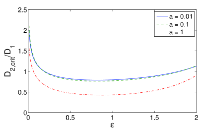
There are similarities and differences between the behaviors of D2,critsubscript𝐷2critD_{2,\rm crit} in 2D and 3D. Figure 9 shows that D2,critsubscript𝐷2critD_{2,\rm crit} from Eq. (82) is not a monotonous function of ϵitalic-ϵ\epsilon, with the qualitative explanation which is the same as in the two-dimensional case.

In contrast to the analogous Eq. (39) in 2D, the rhs of Eq. (82) diverges as ϵ0italic-ϵ0\epsilon\to 0. This divergence reflects the fact that a poink-like target (ϵ=0italic-ϵ0\epsilon=0), which could be found within a finite time in 2D by one-dimensional surface diffusion on the circle, is not detectable in 3D neither by bulk excursions, nor by surface diffusion.
Refer to caption
Figure 9: D2,critsubscript𝐷2critD_{2,\rm crit} as a function of ϵitalic-ϵ\epsilon is computed from Eq. (80) in 3D for three values of a/R𝑎𝑅a/R: 0.010.010.01, 0.10.10.1, and 111. When ϵitalic-ϵ\epsilon approaches π𝜋\pi (the whole surface becomes absorbing), D2,critsubscript𝐷2critD_{2,\rm crit} diverges (not shown). In fact, in this limit, there is no need for a bulk excursion because the target will be found immediately by the surface diffusion. In addition, D2,critsubscript𝐷2critD_{2,\rm crit} also diverges as ϵ0italic-ϵ0\epsilon\to 0 because a point-like target cannot be detected neither by bulk excursions, nor by surface diffusion in 3D.

IV.6.2 When is there an optimal value of the desorption rate λ𝜆\lambda minimizing the search time ?

For the reaction time to be an optimizable function of the desorption rate λ𝜆\lambda, it is necessary to write an additional condition, requiring that the bulk excursions are not ”too favorable” (otherwise, the best strategy is obtained for λ𝜆\lambda\to\infty). A sufficient condition is given by demanding that the search time at zero desorption rate (i.e., without leaving the boundary) is less than the search time at infinite desorption rate

t1(λ=0)<t1(λ).delimited-⟨⟩subscript𝑡1𝜆0delimited-⟨⟩subscript𝑡1𝜆\langle t_{1}(\lambda=0)\rangle<\langle t_{1}(\lambda\to\infty)\rangle. (83)
t1(λ=0)=R2D1(2ln(2/ϵ)1)+O(ϵ),delimited-⟨⟩subscript𝑡1𝜆0superscript𝑅2subscript𝐷122italic-ϵ1𝑂italic-ϵ\langle t_{1}(\lambda=0)\rangle=\frac{R^{2}}{D_{1}}(2\ln(2/\epsilon)-1)+O(\epsilon), (84)

which writes in the physically relevant limit aRmuch-less-than𝑎𝑅a\ll R (using the result of Singer et al. (2006b)):

t1(λ)=πR23ϵD2(1+ϵln(1/ϵ)).delimited-⟨⟩subscript𝑡1𝜆𝜋superscript𝑅23italic-ϵsubscript𝐷21italic-ϵ1italic-ϵ\langle t_{1}(\lambda\to\infty)\rangle=\frac{\pi R^{2}}{3\epsilon D_{2}}\left(1+\epsilon\ln(1/\epsilon)\right). (85)

Finally, this conditions leads, for small ϵitalic-ϵ\epsilon, to

D1D2>3ϵπ(2ln(2/ϵ)1).subscript𝐷1subscript𝐷23italic-ϵ𝜋22italic-ϵ1\frac{D_{1}}{D_{2}}>\frac{3\epsilon}{\pi}(2\ln(2/\epsilon)-1). (86)

Combining the two conditions (82, 86), the search time is found to be optimizable when aRmuch-less-than𝑎𝑅a\ll R and ϵ1much-less-thanitalic-ϵ1\epsilon\ll 1 if

3ϵπ(2ln(2/ϵ)1)<D1D2<π22(2ln(2/ϵ)1).3italic-ϵ𝜋22italic-ϵ1subscript𝐷1subscript𝐷2superscript𝜋2222italic-ϵ1\frac{3\epsilon}{\pi}(2\ln(2/\epsilon)-1)<\frac{D_{1}}{D_{2}}<\frac{\pi^{2}}{2(2\ln(2/\epsilon)-1)}. (87)
Refer to caption
Refer to caption
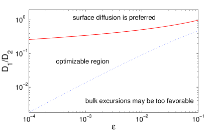
Figure 10: The regions of optimality for the search time in 2D (left) and 3D (right). The lower bound (solid blue line) and upper bound (dashed red line) are given in the limit of aRmuch-less-than𝑎𝑅a\ll R and ϵ1much-less-thanitalic-ϵ1\epsilon\ll 1 by Eqs. (43, 87) in 2D and 3D, respectively. When the ratio D1/D2subscript𝐷1subscript𝐷2D_{1}/D_{2} lies between two curves, the search time t1delimited-⟨⟩subscript𝑡1\langle t_{1}\rangle is optimizable with respect to λ𝜆\lambda. Above the upper bound, surface diffusion is preferred (λ=0𝜆0\lambda=0 is the optimal solution), while below the lower bound, bulk excursions may be ”too favorable” (λ𝜆\lambda\to\infty may give the optimal solution). We recall that the lower bound was obtained from the sufficient condition (83) meaning that the region below the dotted line may still be optimizable.

V Numerical resolution

In the previous sections, we derived the closed matrix forms (25, 65) for the coefficients dnsubscript𝑑𝑛d_{n} in 2D and 3D. These coefficients determine the angular dependence of t1(θ)subscript𝑡1𝜃t_{1}(\theta) through the explicit representations (20, 60) in 2D and 3D, respectively. Although the formulas (25, 65) which are based on the inversion of an infinite-dimensional matrix (IΩQ)𝐼Ω𝑄(I-\Omega Q) remain implicit, a numerical resolution of the problem has become straightforward. In fact, one needs to truncate the infinite-dimensional matrix Q𝑄Q and vectors U𝑈U and U~~𝑈\tilde{U} and to invert the truncated matrix (IΩQ)𝐼Ω𝑄(I-\Omega Q) numerically.

There are six parameters that determine the function t1(θ)subscript𝑡1𝜃t_{1}(\theta): the radius R𝑅R of the disk (sphere), the diffusion coefficients D1subscript𝐷1D_{1} and D2subscript𝐷2D_{2}, the desorption rate λ𝜆\lambda, the size ϵitalic-ϵ\epsilon of the absorbing region, and the distance a𝑎a. From now on, we set the units of length and time by setting R=1𝑅1R=1 and D1=1subscript𝐷11D_{1}=1. Although the distance a𝑎a may take any value from 00 to R𝑅R, the physically interesting case corresponds to the limit of small a𝑎a. As we mentioned previously, the limit a=0𝑎0a=0 exists but trivially leads to searching on the surface, without intermediate bulk excursions. In order to reveal the role of a𝑎a, we consider several values of a𝑎a: 0.0010.0010.001, 0.010.010.01, 0.10.10.1 and 111, the latter corresponding to the specific situation when search is always restarted from the center. Since the diffusion coefficient D2subscript𝐷2D_{2} enters only through the prefactor T𝑇T from Eq. (10), its influence onto the searching time t1subscript𝑡1t_{1} is easy to examine. In what follows, we take three values of D2subscript𝐷2D_{2}: 0.10.10.1, 111 and 101010. The dependence of t1subscript𝑡1t_{1} on the desorption rate λ𝜆\lambda and the size ϵitalic-ϵ\epsilon is the most interesting issue which will be studied below.

In the previous sections, we derived several formulas for computing t1subscript𝑡1t_{1}:

  • explicit representations (20, 60) with the exact expressions (25, 65) for the coefficients;

  • approximations (32, 75) which were derived by neglecting non-diagonal elements of the matrix Q𝑄Q;

  • perturbative formulas (11, 71) which are valid for small ϵitalic-ϵ\epsilon.

For a numerical computation of the coefficients in Eqs. (25, 65), we truncate the infinite-dimensional matrix Q𝑄Q to a finite size N×N𝑁𝑁N\times N and invert the matrix (IΩQ)𝐼Ω𝑄(I-\Omega Q). In order to check the accuracy of this scheme, we compute the coefficients by taking several values of N𝑁N from 101010 to 200200200. For D2=1subscript𝐷21D_{2}=1, ϵ=0.1italic-ϵ0.1\epsilon=0.1, a=0.01𝑎0.01a=0.01 and λ=1𝜆1\lambda=1, the computed mean time t1delimited-⟨⟩subscript𝑡1\langle t_{1}\rangle rapidly converges to a limit. Even the computation with N=10𝑁10N=10 gives the result with four significant digits. Note that other sets of parameters (e.g., larger values of ΩΩ\Omega) may require larger truncation sizes.

VI Conclusion

To conclude, we have presented an exact calculation of the mean first-passage time to a target on the surface of a 2D and 3D spherical domain, for a molecule performing surface-mediated diffusion. The presented approach is based on an integral equation which can be solved analytically, and numerically validated approximation schemes, which provide more tractable expressions of the mean FPT. This minimal model of surface-mediated reactions, which explicitly takes into account the combination of surface and bulk diffusions, shows the importance of correlations induced by the coupling of the switching dynamics to the geometry of the confinement. Indeed, standard MF treatments prove to substantially underestimate the reaction time in this case Benichou et al. (2008), and sometimes even fail to reproduce the proper monotonicity Oshanin et al. (2010). In the context of interfacial systems in confinement, our results show that the reaction time can be minimized as a function of the desorption rate from the surface, which puts forward a general mechanism of enhancement and regulation of chemical reactivity.

Appendix A Another approach in 2D

In this Appendix, we describe another theoretical approach which relies on the explicit form of the Green function of the Poisson equation in 2D case. In particular, the perturbative analysis for small ϵitalic-ϵ\epsilon becomes easier within this approach.

Considering t2subscript𝑡2t_{2} as a source term in the Poisson type equation (1) with absorbing conditions at θ=ϵ𝜃italic-ϵ\theta=\epsilon and θ=2πϵ𝜃2𝜋italic-ϵ\theta=2\pi-\epsilon whose Green function is well known Barton (1989), t1subscript𝑡1t_{1} writes

t1(θ)subscript𝑡1𝜃\displaystyle t_{1}(\theta) =\displaystyle= 1ωsinh(2ω(πϵ))ϵ2πϵsinh(ω(θ<ϵ))sinh(ω(2πϵθ>))[R2D1+λR2D1t2(Ra,θ)]dθ,1𝜔2𝜔𝜋italic-ϵsuperscriptsubscriptitalic-ϵ2𝜋italic-ϵ𝜔subscript𝜃italic-ϵ𝜔2𝜋italic-ϵsubscript𝜃delimited-[]superscript𝑅2subscript𝐷1𝜆superscript𝑅2subscript𝐷1subscript𝑡2𝑅𝑎superscript𝜃differential-dsuperscript𝜃\displaystyle\frac{1}{\omega\sinh(2\omega(\pi-\epsilon))}\int_{\epsilon}^{2\pi-\epsilon}\sinh(\omega(\theta_{<}-\epsilon))\sinh(\omega(2\pi-\epsilon-\theta_{>}))\left[\frac{R^{2}}{D_{1}}+\frac{\lambda R^{2}}{D_{1}}t_{2}(R-a,\theta^{\prime})\right]{\rm d}\theta^{\prime}, (88)

and the notations θ<=min(θ,θ)subscript𝜃𝜃superscript𝜃\theta_{<}=\min(\theta,\theta^{\prime}) and θ>=max(θ,θ)subscript𝜃𝜃superscript𝜃\theta_{>}=\max(\theta,\theta^{\prime}).

Injecting Eq. (5) into Eq. (88) leads to

t1(θ)=ωλsinh(2ω(πϵ))(I(0,θ)(1+λ(α0(Ra)24D2))+λm=1αm(Ra)mI(m,θ)),subscript𝑡1𝜃𝜔𝜆2𝜔𝜋italic-ϵI0𝜃1𝜆subscript𝛼0superscript𝑅𝑎24subscript𝐷2𝜆superscriptsubscript𝑚1subscript𝛼𝑚superscript𝑅𝑎𝑚I𝑚𝜃t_{1}(\theta)=\frac{\omega}{\lambda\sinh(2\omega(\pi-\epsilon))}\left({\rm I}(0,\theta)\left(1+\lambda\left(\alpha_{0}-\frac{(R-a)^{2}}{4D_{2}}\right)\right)+\lambda\sum_{m=1}^{\infty}\alpha_{m}(R-a)^{m}{\rm I}(m,\theta)\right), (89)

where, for m𝑚m integer,

I(m,θ)I𝑚𝜃\displaystyle{\rm I}(m,\theta) \displaystyle\equiv ϵ2πϵsinh(ω(θ<ϵ))sinh(ω(2πϵθ>))cos(mθ)dθsuperscriptsubscriptitalic-ϵ2𝜋italic-ϵ𝜔subscript𝜃italic-ϵ𝜔2𝜋italic-ϵsubscript𝜃𝑚superscript𝜃differential-dsuperscript𝜃\displaystyle\int_{\epsilon}^{2\pi-\epsilon}\sinh(\omega(\theta_{<}-\epsilon))\sinh(\omega(2\pi-\epsilon-\theta_{>}))\cos(m\theta^{\prime}){\rm d}\theta^{\prime} (90)
=\displaystyle= ωω2+m2(cos(mθ)sinh(2ω(πϵ))2cos(mϵ)sinh(ω(πϵ))cosh(ω(θπ))),𝜔superscript𝜔2superscript𝑚2𝑚𝜃2𝜔𝜋italic-ϵ2𝑚italic-ϵ𝜔𝜋italic-ϵ𝜔𝜃𝜋\displaystyle\frac{\omega}{\omega^{2}+m^{2}}\left(\cos(m\theta)\sinh(2\omega(\pi-\epsilon))-2\cos(m\epsilon)\sinh(\omega(\pi-\epsilon))\cosh(\omega(\theta-\pi))\right),

so that

t1(θ)subscript𝑡1𝜃\displaystyle t_{1}(\theta) =\displaystyle= 1λ+α0(Ra)24D2+ω2m=1αmω2+m2(Ra)mcos(mθ)1𝜆subscript𝛼0superscript𝑅𝑎24subscript𝐷2superscript𝜔2superscriptsubscript𝑚1subscript𝛼𝑚superscript𝜔2superscript𝑚2superscript𝑅𝑎𝑚𝑚𝜃\displaystyle\frac{1}{\lambda}+\alpha_{0}-\frac{(R-a)^{2}}{4D_{2}}+\omega^{2}\sum_{m=1}^{\infty}\frac{\alpha_{m}}{\omega^{2}+m^{2}}(R-a)^{m}\cos(m\theta) (91)
\displaystyle- cosh(ω(θπ))cosh(ω(πϵ))(1λ+α0(Ra)24D2+ω2m=1αmω2+m2(Ra)mcos(mϵ)).𝜔𝜃𝜋𝜔𝜋italic-ϵ1𝜆subscript𝛼0superscript𝑅𝑎24subscript𝐷2superscript𝜔2superscriptsubscript𝑚1subscript𝛼𝑚superscript𝜔2superscript𝑚2superscript𝑅𝑎𝑚𝑚italic-ϵ\displaystyle\frac{\cosh(\omega(\theta-\pi))}{\cosh(\omega(\pi-\epsilon))}\left(\frac{1}{\lambda}+\alpha_{0}-\frac{(R-a)^{2}}{4D_{2}}+\omega^{2}\sum_{m=1}^{\infty}\frac{\alpha_{m}}{\omega^{2}+m^{2}}(R-a)^{m}\cos(m\epsilon)\right).

Substituting Eq. (91) into Eq. (7) gives

Stanh(ω(πϵ))ωπ=ϵπλα0+1ϵπ+λ(R24D2(1ϵπ)(Ra)24D2)λω2πm=1αmω2+m2(Ra)msin(mϵ)m,𝑆𝜔𝜋italic-ϵ𝜔𝜋italic-ϵ𝜋𝜆subscript𝛼01italic-ϵ𝜋𝜆superscript𝑅24subscript𝐷21italic-ϵ𝜋superscript𝑅𝑎24subscript𝐷2𝜆superscript𝜔2𝜋superscriptsubscript𝑚1subscript𝛼𝑚superscript𝜔2superscript𝑚2superscript𝑅𝑎𝑚𝑚italic-ϵ𝑚\displaystyle S\frac{\tanh(\omega(\pi-\epsilon))}{\omega\pi}=-\frac{\epsilon}{\pi}\lambda\alpha_{0}+1-\frac{\epsilon}{\pi}+\lambda\left(\frac{R^{2}}{4D_{2}}-\left(1-\frac{\epsilon}{\pi}\right)\frac{(R-a)^{2}}{4D_{2}}\right)-\frac{\lambda\omega^{2}}{\pi}\sum_{m=1}^{\infty}\frac{\alpha_{m}}{\omega^{2}+m^{2}}(R-a)^{m}\frac{\sin(m\epsilon)}{m}, (92)

and

λ(Rnω2ω2+n2(1ϵπ)(Ra)n)αn=𝜆superscript𝑅𝑛superscript𝜔2superscript𝜔2superscript𝑛21italic-ϵ𝜋superscript𝑅𝑎𝑛subscript𝛼𝑛absent\displaystyle\lambda\left(R^{n}-\frac{\omega^{2}}{\omega^{2}+n^{2}}\left(1-\frac{\epsilon}{\pi}\right)(R-a)^{n}\right)\alpha_{n}= (93)
\displaystyle- 2sin(nϵ)nπ(1+λ(α0(Ra)24D2))2𝑛italic-ϵ𝑛𝜋1𝜆subscript𝛼0superscript𝑅𝑎24subscript𝐷2\displaystyle\frac{2\sin(n\epsilon)}{n\pi}\left(1+\lambda\left(\alpha_{0}-\frac{(R-a)^{2}}{4D_{2}}\right)\right)
\displaystyle- λω2π(mnαmω2+m2(Ra)msin((mn)ϵ)mn+m=1αmω2+m2(Ra)msin((m+n)ϵ)m+n)𝜆superscript𝜔2𝜋subscript𝑚𝑛subscript𝛼𝑚superscript𝜔2superscript𝑚2superscript𝑅𝑎𝑚𝑚𝑛italic-ϵ𝑚𝑛superscriptsubscript𝑚1subscript𝛼𝑚superscript𝜔2superscript𝑚2superscript𝑅𝑎𝑚𝑚𝑛italic-ϵ𝑚𝑛\displaystyle\frac{\lambda\omega^{2}}{\pi}\left(\sum_{m\neq n}\frac{\alpha_{m}}{\omega^{2}+m^{2}}(R-a)^{m}\frac{\sin((m-n)\epsilon)}{m-n}+\sum_{m=1}^{\infty}\frac{\alpha_{m}}{\omega^{2}+m^{2}}(R-a)^{m}\frac{\sin((m+n)\epsilon)}{m+n}\right)
\displaystyle- 2tanh(ω(πϵ))π(ω2+n2)S(ωcos(nϵ)nsin(nϵ)tanh(ω(πϵ))),2𝜔𝜋italic-ϵ𝜋superscript𝜔2superscript𝑛2𝑆𝜔𝑛italic-ϵ𝑛𝑛italic-ϵ𝜔𝜋italic-ϵ\displaystyle\frac{2\tanh(\omega(\pi-\epsilon))}{\pi(\omega^{2}+n^{2})}S\left(\omega\cos(n\epsilon)-\frac{n\sin(n\epsilon)}{\tanh(\omega(\pi-\epsilon))}\right),

where

S1+λ(α0(Ra)24D2)+λω2m=1αmω2+m2(Ra)mcos(mϵ).𝑆1𝜆subscript𝛼0superscript𝑅𝑎24subscript𝐷2𝜆superscript𝜔2superscriptsubscript𝑚1subscript𝛼𝑚superscript𝜔2superscript𝑚2superscript𝑅𝑎𝑚𝑚italic-ϵS\equiv 1+\lambda\left(\alpha_{0}-\frac{(R-a)^{2}}{4D_{2}}\right)+\lambda\omega^{2}\sum_{m=1}^{\infty}\frac{\alpha_{m}}{\omega^{2}+m^{2}}(R-a)^{m}\cos(m\epsilon). (94)

Eq. (92) can be rearranged into

(α0R24D2)(ϵπ+tanh(ω(πϵ))πω)subscript𝛼0superscript𝑅24subscript𝐷2italic-ϵ𝜋𝜔𝜋italic-ϵ𝜋𝜔\displaystyle(\alpha_{0}-\frac{R^{2}}{4D_{2}})\left(\frac{\epsilon}{\pi}+\frac{\tanh(\omega(\pi-\epsilon))}{\pi\omega}\right) =\displaystyle= (1λ+(R24D2(Ra)24D2))(1ϵπtanh(ω(πϵ))πω)1𝜆superscript𝑅24subscript𝐷2superscript𝑅𝑎24subscript𝐷21italic-ϵ𝜋𝜔𝜋italic-ϵ𝜋𝜔\displaystyle\left(\frac{1}{\lambda}+\left(\frac{R^{2}}{4D_{2}}-\frac{(R-a)^{2}}{4D_{2}}\right)\right)\left(1-\frac{\epsilon}{\pi}-\frac{\tanh(\omega(\pi-\epsilon))}{\pi\omega}\right) (95)
\displaystyle- ωπn=1(Ra)nω2+n2(tanh(ω(πϵ))cos(nϵ)+ωnsin(nϵ))αn,𝜔𝜋superscriptsubscript𝑛1superscript𝑅𝑎𝑛superscript𝜔2superscript𝑛2𝜔𝜋italic-ϵ𝑛italic-ϵ𝜔𝑛𝑛italic-ϵsubscript𝛼𝑛\displaystyle\frac{\omega}{\pi}\sum_{n=1}^{\infty}\frac{(R-a)^{n}}{\omega^{2}+n^{2}}\left(\tanh(\omega(\pi-\epsilon))\cos(n\epsilon)+\frac{\omega}{n}\sin(n\epsilon)\right)\alpha_{n},

and Eq. (93) into

(Rnω2ω2+n2(1ϵπ)(Ra)n)αn=superscript𝑅𝑛superscript𝜔2superscript𝜔2superscript𝑛21italic-ϵ𝜋superscript𝑅𝑎𝑛subscript𝛼𝑛absent\displaystyle\left(R^{n}-\frac{\omega^{2}}{\omega^{2}+n^{2}}\left(1-\frac{\epsilon}{\pi}\right)(R-a)^{n}\right)\alpha_{n}=
2πn(α0R24D2+T)(ω2ω2+n2sin(nϵ)+nωω2+n2tanh(ω(πϵ))cos(nϵ))2𝜋𝑛subscript𝛼0superscript𝑅24subscript𝐷2𝑇superscript𝜔2superscript𝜔2superscript𝑛2𝑛italic-ϵ𝑛𝜔superscript𝜔2superscript𝑛2𝜔𝜋italic-ϵ𝑛italic-ϵ\displaystyle-\frac{2}{\pi n}(\alpha_{0}-\frac{R^{2}}{4D_{2}}+T)\left(\frac{\omega^{2}}{\omega^{2}+n^{2}}\sin(n\epsilon)+\frac{n\omega}{\omega^{2}+n^{2}}\tanh(\omega(\pi-\epsilon))\cos(n\epsilon)\right)
2ω2π(ω2+n2)m=1αm(Ra)mω2+m2cos(mϵ)(ωcos(nϵ)tanh(ω(πϵ))nsin(nϵ))2superscript𝜔2𝜋superscript𝜔2superscript𝑛2superscriptsubscript𝑚1subscript𝛼𝑚superscript𝑅𝑎𝑚superscript𝜔2superscript𝑚2𝑚italic-ϵ𝜔𝑛italic-ϵ𝜔𝜋italic-ϵ𝑛𝑛italic-ϵ\displaystyle-\frac{2\omega^{2}}{\pi(\omega^{2}+n^{2})}\sum_{m=1}^{\infty}\alpha_{m}\frac{(R-a)^{m}}{\omega^{2}+m^{2}}\cos(m\epsilon)(\omega\cos(n\epsilon)\tanh(\omega(\pi-\epsilon))-n\sin(n\epsilon))
ω2π(mnαmω2+m2(Ra)msin((mn)ϵ)mn+m=1αmω2+m2(Ra)msin((m+n)ϵ)m+n).superscript𝜔2𝜋subscript𝑚𝑛subscript𝛼𝑚superscript𝜔2superscript𝑚2superscript𝑅𝑎𝑚𝑚𝑛italic-ϵ𝑚𝑛superscriptsubscript𝑚1subscript𝛼𝑚superscript𝜔2superscript𝑚2superscript𝑅𝑎𝑚𝑚𝑛italic-ϵ𝑚𝑛\displaystyle-\frac{\omega^{2}}{\pi}\left(\sum_{m\neq n}\frac{\alpha_{m}}{\omega^{2}+m^{2}}(R-a)^{m}\frac{\sin((m-n)\epsilon)}{m-n}+\sum_{m=1}^{\infty}\frac{\alpha_{m}}{\omega^{2}+m^{2}}(R-a)^{m}\frac{\sin((m+n)\epsilon)}{m+n}\right). (96)

A.1 Particular case λ=0𝜆0\lambda=0

In this case, the previous equations can be solved exactly, leading to

α0R24D2=13R2D1(πϵ)3π,subscript𝛼0superscript𝑅24subscript𝐷213superscript𝑅2subscript𝐷1superscript𝜋italic-ϵ3𝜋\alpha_{0}-\frac{R^{2}}{4D_{2}}=\frac{1}{3}\frac{R^{2}}{D_{1}}\frac{(\pi-\epsilon)^{3}}{\pi}, (97)

and

αn=2πR2D1n(πϵ)cos(nϵ)+sin(nϵ)n31Rn.subscript𝛼𝑛2𝜋superscript𝑅2subscript𝐷1𝑛𝜋italic-ϵ𝑛italic-ϵ𝑛italic-ϵsuperscript𝑛31superscript𝑅𝑛\alpha_{n}=-\frac{2}{\pi}\frac{R^{2}}{D_{1}}\frac{n(\pi-\epsilon)\cos(n\epsilon)+\sin(n\epsilon)}{n^{3}}\frac{1}{R^{n}}. (98)

We note that the particular case a=0𝑎0a=0 is also described by these expressions, although it does not seem to be clear from Eqs. (92)-(93).

A.2 Particular case a=R𝑎𝑅a=R

Here again, Eqs. (92)-(93) can be solved exactly, and give :

α0R24D2=(1λ+R24D2)1ϵπtanh(ω(πϵ))πωϵπ+tanh(ω(πϵ))πω,subscript𝛼0superscript𝑅24subscript𝐷21𝜆superscript𝑅24subscript𝐷21italic-ϵ𝜋𝜔𝜋italic-ϵ𝜋𝜔italic-ϵ𝜋𝜔𝜋italic-ϵ𝜋𝜔\alpha_{0}-\frac{R^{2}}{4D_{2}}=\left(\frac{1}{\lambda}+\frac{R^{2}}{4D_{2}}\right)\frac{1-\frac{\epsilon}{\pi}-\frac{\tanh(\omega(\pi-\epsilon))}{\pi\omega}}{\frac{\epsilon}{\pi}+\frac{\tanh(\omega(\pi-\epsilon))}{\pi\omega}}, (99)

and

αn=2π(1λ+R24D2)ωω2+n2ωnsin(nϵ)+tanh(ω(πϵ))cos(nϵ)ϵπ+tanh(ω(πϵ))πω1Rn.subscript𝛼𝑛2𝜋1𝜆superscript𝑅24subscript𝐷2𝜔superscript𝜔2superscript𝑛2𝜔𝑛𝑛italic-ϵ𝜔𝜋italic-ϵ𝑛italic-ϵitalic-ϵ𝜋𝜔𝜋italic-ϵ𝜋𝜔1superscript𝑅𝑛\alpha_{n}=-\frac{2}{\pi}\left(\frac{1}{\lambda}+\frac{R^{2}}{4D_{2}}\right)\frac{\omega}{\omega^{2}+n^{2}}\frac{\frac{\omega}{n}\sin(n\epsilon)+\tanh(\omega(\pi-\epsilon))\cos(n\epsilon)}{\frac{\epsilon}{\pi}+\frac{\tanh(\omega(\pi-\epsilon))}{\pi\omega}}\frac{1}{R^{n}}. (100)

A.3 Perturbative approach

Expanding α0subscript𝛼0\alpha_{0} and αnsubscript𝛼𝑛\alpha_{n} in powers of ϵitalic-ϵ\epsilon

α0=α0(0)+α0(1)ϵ+α0(2)ϵ2+andαn=αn(0)+αn(1)ϵ+αn(2)ϵ2+subscript𝛼0superscriptsubscript𝛼00superscriptsubscript𝛼01italic-ϵsuperscriptsubscript𝛼02superscriptitalic-ϵ2andsubscript𝛼𝑛superscriptsubscript𝛼𝑛0superscriptsubscript𝛼𝑛1italic-ϵsuperscriptsubscript𝛼𝑛2superscriptitalic-ϵ2\alpha_{0}=\alpha_{0}^{(0)}+\alpha_{0}^{(1)}\epsilon+\alpha_{0}^{(2)}\epsilon^{2}+\dots\;\;{\rm and}\;\;\alpha_{n}=\alpha_{n}^{(0)}+\alpha_{n}^{(1)}\epsilon+\alpha_{n}^{(2)}\epsilon^{2}+\dots (101)

Eqs. (92)-(93) lead, after lengthy calculations, to

α0=R24D2+ω2T{(2m=11ω2(1xm)+m2)πϵ+(1+2ω2m=11xmω2(1xm)+m2)ϵ2}+,αn=ω2TRn(ω2(1xn)+n2){2+n2ϵ2+}.formulae-sequencesubscript𝛼0superscript𝑅24subscript𝐷2superscript𝜔2𝑇2superscriptsubscript𝑚11superscript𝜔21superscript𝑥𝑚superscript𝑚2𝜋italic-ϵ12superscript𝜔2superscriptsubscript𝑚11superscript𝑥𝑚superscript𝜔21superscript𝑥𝑚superscript𝑚2superscriptitalic-ϵ2subscript𝛼𝑛superscript𝜔2𝑇superscript𝑅𝑛superscript𝜔21superscript𝑥𝑛superscript𝑛22superscript𝑛2superscriptitalic-ϵ2\begin{split}\alpha_{0}&=\frac{R^{2}}{4D_{2}}+\omega^{2}T\left\{\left(2\sum_{m=1}^{\infty}\frac{1}{\omega^{2}\left(1-x^{m}\right)+m^{2}}\right)-\pi\epsilon+\left(1+2\omega^{2}\sum_{m=1}^{\infty}\frac{1-x^{m}}{\omega^{2}\left(1-x^{m}\right)+m^{2}}\right)\epsilon^{2}\right\}+\dots,\\ \alpha_{n}&=\frac{\omega^{2}T}{R^{n}(\omega^{2}(1-x^{n})+n^{2})}\left\{-2+n^{2}\epsilon^{2}+\dots\right\}.\end{split} (102)

Appendix B A second integral equation satified by t1subscript𝑡1t_{1} in the 2D case

Using Eq. (7) for the Fourier coefficients in Eq. (91) leads to a second integral equation satisfied by t1subscript𝑡1t_{1}

t1(θ)=T(1cosh(ω(πθ))cosh(ω(πϵ)))+ϵ2πϵt1(α)(J(θ,α)cosh(ω(πθ))cosh(ω(πϵ))J(ϵ,α))dα,subscript𝑡1𝜃𝑇1𝜔𝜋𝜃𝜔𝜋italic-ϵsuperscriptsubscriptitalic-ϵ2𝜋italic-ϵsubscript𝑡1𝛼𝐽𝜃𝛼𝜔𝜋𝜃𝜔𝜋italic-ϵ𝐽italic-ϵ𝛼differential-d𝛼\displaystyle t_{1}(\theta)=T\left(1-\frac{\cosh(\omega(\pi-\theta))}{\cosh(\omega(\pi-\epsilon))}\right)+\int_{\epsilon}^{2\pi-\epsilon}t_{1}(\alpha)\left(J(\theta,\alpha)-\frac{\cosh(\omega(\pi-\theta))}{\cosh(\omega(\pi-\epsilon))}J(\epsilon,\alpha)\right){\rm d}\alpha, (103)

where

J(θ,α)12π+1πn=1ω2ω2+n2(1aR)ncos(nθ)cos(nα).𝐽𝜃𝛼12𝜋1𝜋superscriptsubscript𝑛1superscript𝜔2superscript𝜔2superscript𝑛2superscript1𝑎𝑅𝑛𝑛𝜃𝑛𝛼J(\theta,\alpha)\equiv\frac{1}{2\pi}+\frac{1}{\pi}\sum_{n=1}^{\infty}\frac{\omega^{2}}{\omega^{2}+n^{2}}\left(1-\frac{a}{R}\right)^{n}\cos(n\theta)\cos(n\alpha). (104)

This equation is especially well adapted to local expansions of t1(θ)subscript𝑡1𝜃t_{1}(\theta) in the vicinity of aRsimilar-to-or-equals𝑎𝑅a\simeq R, but it can also be rearranged into the following integral equation, useful when aRmuch-less-than𝑎𝑅a\ll R :

t1(θ)subscript𝑡1𝜃\displaystyle t_{1}(\theta) =\displaystyle= T(1cosh(ω(πθ))cosh(ω(πϵ)))+ωsinh(2ω(πϵ))ϵ2πϵt1(θ)sinh(ω(θ<ϵ))sinh(ω(2πϵθ>))dθ+𝑇1𝜔𝜋𝜃𝜔𝜋italic-ϵlimit-from𝜔2𝜔𝜋italic-ϵsuperscriptsubscriptitalic-ϵ2𝜋italic-ϵsubscript𝑡1superscript𝜃𝜔subscript𝜃italic-ϵ𝜔2𝜋italic-ϵsubscript𝜃differential-dsuperscript𝜃\displaystyle T\left(1-\frac{\cosh(\omega(\pi-\theta))}{\cosh(\omega(\pi-\epsilon))}\right)+\frac{\omega}{\sinh(2\omega(\pi-\epsilon))}\int_{\epsilon}^{2\pi-\epsilon}t_{1}(\theta^{\prime})\sinh(\omega(\theta_{<}-\epsilon))\sinh(\omega(2\pi-\epsilon-\theta_{>})){\rm d}\theta^{\prime}+ (105)
+\displaystyle+ ϵ2πϵt1(α)(J~(θ,α)cosh(ω(πθ))cosh(ω(πϵ))J~(ϵ,α))dα,superscriptsubscriptitalic-ϵ2𝜋italic-ϵsubscript𝑡1𝛼~𝐽𝜃𝛼𝜔𝜋𝜃𝜔𝜋italic-ϵ~𝐽italic-ϵ𝛼differential-d𝛼\displaystyle\int_{\epsilon}^{2\pi-\epsilon}t_{1}(\alpha)\left(\widetilde{J}(\theta,\alpha)-\frac{\cosh(\omega(\pi-\theta))}{\cosh(\omega(\pi-\epsilon))}\widetilde{J}(\epsilon,\alpha)\right){\rm d}\alpha,

where

J~(θ,α)1πn=1ω2ω2+n2((1aR)n1)cos(nθ)cos(nα).~𝐽𝜃𝛼1𝜋superscriptsubscript𝑛1superscript𝜔2superscript𝜔2superscript𝑛2superscript1𝑎𝑅𝑛1𝑛𝜃𝑛𝛼\widetilde{J}(\theta,\alpha)\equiv\frac{1}{\pi}\sum_{n=1}^{\infty}\frac{\omega^{2}}{\omega^{2}+n^{2}}\left(\left(1-\frac{a}{R}\right)^{n}-1\right)\cos(n\theta)\cos(n\alpha). (106)

Appendix C Computation of Iϵ(m,n)subscript𝐼italic-ϵ𝑚𝑛I_{\epsilon}(m,n) in 3D

In this Appendix, we provide the explicit formula for the matrix Iϵ(m,n)subscript𝐼italic-ϵ𝑚𝑛I_{\epsilon}(m,n) in 3D case. Although technical, this is an important result for a numerical computation because it allows one to avoid an approximate integration in Eq. (64) which otherwise could be a significant source of numerical errors. The formula (112) for non-diagonal elements is somewhat elementary, while the derivation for diagonal elements seems to be original.

Non-diagonal elements

The Legendre polynomials satisfy

ddx[(1x2)ddxPn(x)]+n(n+1)Pn(x)=0,𝑑𝑑𝑥delimited-[]1superscript𝑥2𝑑𝑑𝑥subscript𝑃𝑛𝑥𝑛𝑛1subscript𝑃𝑛𝑥0\frac{d}{dx}\biggl{[}(1-x^{2})\frac{d}{dx}P_{n}(x)\biggr{]}+n(n+1)P_{n}(x)=0, (107)

from which

ab𝑑xPn(x)=[(1x2)Pn(x)]abn(n+1)(n>0).superscriptsubscript𝑎𝑏differential-d𝑥subscript𝑃𝑛𝑥superscriptsubscriptdelimited-[]1superscript𝑥2subscriptsuperscript𝑃𝑛𝑥𝑎𝑏𝑛𝑛1𝑛0\int\limits_{a}^{b}dxP_{n}(x)=-\frac{\bigl{[}(1-x^{2})P^{\prime}_{n}(x)\bigr{]}_{a}^{b}}{n(n+1)}\hskip 14.22636pt(n>0). (108)

and

ab𝑑xPm(x)Pn(x)=[(1x2)[Pm(x)Pn(x)Pn(x)Pm(x)]]abm(m+1)n(n+1)(mn).superscriptsubscript𝑎𝑏differential-d𝑥subscript𝑃𝑚𝑥subscript𝑃𝑛𝑥superscriptsubscriptdelimited-[]1superscript𝑥2delimited-[]subscript𝑃𝑚𝑥subscriptsuperscript𝑃𝑛𝑥subscript𝑃𝑛𝑥subscriptsuperscript𝑃𝑚𝑥𝑎𝑏𝑚𝑚1𝑛𝑛1𝑚𝑛\int\limits_{a}^{b}dxP_{m}(x)P_{n}(x)=\frac{\bigl{[}(1-x^{2})[P_{m}(x)P^{\prime}_{n}(x)-P_{n}(x)P^{\prime}_{m}(x)]\bigr{]}_{a}^{b}}{m(m+1)-n(n+1)}\hskip 14.22636pt(m\neq n). (109)

Since

(1x2)Pn(x)=nxPn(x)+nPn1(x)=(n+1)xPn(x)(n+1)Pn+1(x),1superscript𝑥2subscriptsuperscript𝑃𝑛𝑥𝑛𝑥subscript𝑃𝑛𝑥𝑛subscript𝑃𝑛1𝑥𝑛1𝑥subscript𝑃𝑛𝑥𝑛1subscript𝑃𝑛1𝑥(1-x^{2})P^{\prime}_{n}(x)=-nxP_{n}(x)+nP_{n-1}(x)=(n+1)xP_{n}(x)-(n+1)P_{n+1}(x), (110)

we find

ab𝑑xPn(x)=[xPn(x)Pn1(x)]abn+1(n>0)superscriptsubscript𝑎𝑏differential-d𝑥subscript𝑃𝑛𝑥superscriptsubscriptdelimited-[]𝑥subscript𝑃𝑛𝑥subscript𝑃𝑛1𝑥𝑎𝑏𝑛1𝑛0\int\limits_{a}^{b}dxP_{n}(x)=\frac{\bigl{[}xP_{n}(x)-P_{n-1}(x)\bigr{]}_{a}^{b}}{n+1}\hskip 14.22636pt(n>0) (111)

and

ab𝑑xPm(x)Pn(x)=[(mn)xPm(x)Pn(x)+nPn1(x)Pm(x)mPm1(x)Pn(x)]]abm(m+1)n(n+1)(mn).\int\limits_{a}^{b}dxP_{m}(x)P_{n}(x)=\frac{\bigl{[}(m-n)xP_{m}(x)P_{n}(x)+nP_{n-1}(x)P_{m}(x)-mP_{m-1}(x)P_{n}(x)]\bigr{]}_{a}^{b}}{m(m+1)-n(n+1)}\hskip 14.22636pt(m\neq n). (112)

From the above formulas, we get

Iϵ(m,n)=m(nm)uPm(u)Pn(u)+(m+1)Pm(u)Pn1(u)(n+1)Pn(u)Pm1(u)(n+1)[m(m+1)n(n+1)],u=cosϵ(mn).formulae-sequencesubscript𝐼italic-ϵ𝑚𝑛𝑚𝑛𝑚𝑢subscript𝑃𝑚𝑢subscript𝑃𝑛𝑢𝑚1subscript𝑃𝑚𝑢subscript𝑃𝑛1𝑢𝑛1subscript𝑃𝑛𝑢subscript𝑃𝑚1𝑢𝑛1delimited-[]𝑚𝑚1𝑛𝑛1𝑢italic-ϵ𝑚𝑛\begin{split}I_{\epsilon}(m,n)&=m\frac{(n-m)uP_{m}(u)P_{n}(u)+(m+1)P_{m}(u)P_{n-1}(u)-(n+1)P_{n}(u)P_{m-1}(u)}{(n+1)[m(m+1)-n(n+1)]},\\ u&=\cos\epsilon~{}~{}~{}(m\neq n).\\ \end{split} (113)

Diagonal elements

We denote

Kn=ab𝑑xPn2(x).subscript𝐾𝑛superscriptsubscript𝑎𝑏differential-d𝑥superscriptsubscript𝑃𝑛2𝑥K_{n}=\int\limits_{a}^{b}dxP_{n}^{2}(x). (114)

Using the relation

Pn(x)=2n1nxPn1(x)n1nPn2(x),subscript𝑃𝑛𝑥2𝑛1𝑛𝑥subscript𝑃𝑛1𝑥𝑛1𝑛subscript𝑃𝑛2𝑥P_{n}(x)=\frac{2n-1}{n}xP_{n-1}(x)-\frac{n-1}{n}P_{n-2}(x), (115)

we obtain

Kn=2n1nab𝑑xxPn1(x)Pn(x)n1nab𝑑xPn2(x)Pn(x).subscript𝐾𝑛2𝑛1𝑛superscriptsubscript𝑎𝑏differential-d𝑥𝑥subscript𝑃𝑛1𝑥subscript𝑃𝑛𝑥𝑛1𝑛superscriptsubscript𝑎𝑏differential-d𝑥subscript𝑃𝑛2𝑥subscript𝑃𝑛𝑥K_{n}=\frac{2n-1}{n}\int\limits_{a}^{b}dxxP_{n-1}(x)P_{n}(x)-\frac{n-1}{n}\int\limits_{a}^{b}dxP_{n-2}(x)P_{n}(x). (116)

The second integral is given by Eq. (112). In order to compute the first one, we consider

0=abdx{xPn1(x)[ddx[(1x2)ddxPn(x)]+n(n+1)Pn(x)]xPn(x)[ddx[(1x2)ddxPn1(x)]+(n1)nPn1(x)]}=2nab𝑑xxPn1(x)Pn(x)+[xPn1(x)(1x2)Pn(x)xPn(x)(1x2)Pn1(x)]abab𝑑x(1x2)[Pn(x)Pn1(x)Pn1(x)Pn(x)].0superscriptsubscript𝑎𝑏𝑑𝑥𝑥subscript𝑃𝑛1𝑥delimited-[]𝑑𝑑𝑥delimited-[]1superscript𝑥2𝑑𝑑𝑥subscript𝑃𝑛𝑥𝑛𝑛1subscript𝑃𝑛𝑥𝑥subscript𝑃𝑛𝑥delimited-[]𝑑𝑑𝑥delimited-[]1superscript𝑥2𝑑𝑑𝑥subscript𝑃𝑛1𝑥𝑛1𝑛subscript𝑃𝑛1𝑥2𝑛superscriptsubscript𝑎𝑏differential-d𝑥𝑥subscript𝑃𝑛1𝑥subscript𝑃𝑛𝑥superscriptsubscriptdelimited-[]𝑥subscript𝑃𝑛1𝑥1superscript𝑥2subscriptsuperscript𝑃𝑛𝑥𝑥subscript𝑃𝑛𝑥1superscript𝑥2subscriptsuperscript𝑃𝑛1𝑥𝑎𝑏superscriptsubscript𝑎𝑏differential-d𝑥1superscript𝑥2delimited-[]subscriptsuperscript𝑃𝑛𝑥subscript𝑃𝑛1𝑥subscriptsuperscript𝑃𝑛1𝑥subscript𝑃𝑛𝑥\begin{split}0&=\int\limits_{a}^{b}dx\biggl{\{}xP_{n-1}(x)\biggl{[}\frac{d}{dx}\biggl{[}(1-x^{2})\frac{d}{dx}P_{n}(x)\biggr{]}+n(n+1)P_{n}(x)\biggr{]}\\ &-xP_{n}(x)\biggl{[}\frac{d}{dx}\biggl{[}(1-x^{2})\frac{d}{dx}P_{n-1}(x)\biggr{]}+(n-1)nP_{n-1}(x)\biggr{]}\biggr{\}}\\ &=2n\int\limits_{a}^{b}dxxP_{n-1}(x)P_{n}(x)+\biggl{[}xP_{n-1}(x)(1-x^{2})P^{\prime}_{n}(x)-xP_{n}(x)(1-x^{2})P^{\prime}_{n-1}(x)\biggr{]}_{a}^{b}\\ &-\int\limits_{a}^{b}dx(1-x^{2})\bigl{[}P^{\prime}_{n}(x)P_{n-1}(x)-P^{\prime}_{n-1}(x)P_{n}(x)\bigr{]}.\\ \end{split} (117)

The last integral can be written as

J=ab𝑑x(1x2)Pn2(x)(Pn1(x)/Pn(x))=[(1x2)Pn1(x)Pn(x)]abab𝑑x(Pn1(x)/Pn(x))[2xPn2(x)+2(1x2)Pn(x)Pn(x)]=[(1x2)Pn1(x)Pn(x)]ab2ab𝑑x[xPn1(x)Pn(x)+(1x2)Pn(x)Pn1(x)].𝐽superscriptsubscript𝑎𝑏differential-d𝑥1superscript𝑥2superscriptsubscript𝑃𝑛2𝑥superscriptsubscript𝑃𝑛1𝑥subscript𝑃𝑛𝑥superscriptsubscriptdelimited-[]1superscript𝑥2subscript𝑃𝑛1𝑥subscript𝑃𝑛𝑥𝑎𝑏superscriptsubscript𝑎𝑏differential-d𝑥subscript𝑃𝑛1𝑥subscript𝑃𝑛𝑥delimited-[]2𝑥superscriptsubscript𝑃𝑛2𝑥21superscript𝑥2subscriptsuperscript𝑃𝑛𝑥subscript𝑃𝑛𝑥superscriptsubscriptdelimited-[]1superscript𝑥2subscript𝑃𝑛1𝑥subscript𝑃𝑛𝑥𝑎𝑏2superscriptsubscript𝑎𝑏differential-d𝑥delimited-[]𝑥subscript𝑃𝑛1𝑥subscript𝑃𝑛𝑥1superscript𝑥2subscriptsuperscript𝑃𝑛𝑥subscript𝑃𝑛1𝑥\begin{split}J&=\int\limits_{a}^{b}dx(1-x^{2})P_{n}^{2}(x)(P_{n-1}(x)/P_{n}(x))^{\prime}=\bigl{[}(1-x^{2})P_{n-1}(x)P_{n}(x)\bigr{]}_{a}^{b}\\ &-\int\limits_{a}^{b}dx(P_{n-1}(x)/P_{n}(x))\bigl{[}-2xP_{n}^{2}(x)+2(1-x^{2})P^{\prime}_{n}(x)P_{n}(x)\bigr{]}\\ &=\bigl{[}(1-x^{2})P_{n-1}(x)P_{n}(x)\bigr{]}_{a}^{b}-2\int\limits_{a}^{b}dx\bigl{[}-xP_{n-1}(x)P_{n}(x)+(1-x^{2})P^{\prime}_{n}(x)P_{n-1}(x)\bigr{]}.\\ \end{split} (118)

In the last term, we substitute (1x2)Pn(x)1superscript𝑥2subscriptsuperscript𝑃𝑛𝑥(1-x^{2})P^{\prime}_{n}(x) to get

J=[(1x2)Pn1(x)Pn(x)]ab+2ab𝑑xxPn1(x)Pn(x)2ab𝑑x[nxPn(x)+nPn1(x)]Pn1(x).𝐽superscriptsubscriptdelimited-[]1superscript𝑥2subscript𝑃𝑛1𝑥subscript𝑃𝑛𝑥𝑎𝑏2superscriptsubscript𝑎𝑏differential-d𝑥𝑥subscript𝑃𝑛1𝑥subscript𝑃𝑛𝑥2superscriptsubscript𝑎𝑏differential-d𝑥delimited-[]𝑛𝑥subscript𝑃𝑛𝑥𝑛subscript𝑃𝑛1𝑥subscript𝑃𝑛1𝑥J=\bigl{[}(1-x^{2})P_{n-1}(x)P_{n}(x)\bigr{]}_{a}^{b}+2\int\limits_{a}^{b}dxxP_{n-1}(x)P_{n}(x)-2\int\limits_{a}^{b}dx\bigl{[}-nxP_{n}(x)+nP_{n-1}(x)\bigr{]}P_{n-1}(x). (119)

Bringing these results together, we get

0=2nab𝑑xxPn1(x)Pn(x)+[xPn1(x)(1x2)Pn(x)xPn(x)(1x2)Pn1(x)]ab+[(1x2)Pn1(x)Pn(x)]ab+2ab𝑑xxPn1(x)Pn(x)2ab𝑑x[nxPn(x)+nPn1(x)]Pn1(x)02𝑛superscriptsubscript𝑎𝑏differential-d𝑥𝑥subscript𝑃𝑛1𝑥subscript𝑃𝑛𝑥superscriptsubscriptdelimited-[]𝑥subscript𝑃𝑛1𝑥1superscript𝑥2subscriptsuperscript𝑃𝑛𝑥𝑥subscript𝑃𝑛𝑥1superscript𝑥2subscriptsuperscript𝑃𝑛1𝑥𝑎𝑏superscriptsubscriptdelimited-[]1superscript𝑥2subscript𝑃𝑛1𝑥subscript𝑃𝑛𝑥𝑎𝑏2superscriptsubscript𝑎𝑏differential-d𝑥𝑥subscript𝑃𝑛1𝑥subscript𝑃𝑛𝑥2superscriptsubscript𝑎𝑏differential-d𝑥delimited-[]𝑛𝑥subscript𝑃𝑛𝑥𝑛subscript𝑃𝑛1𝑥subscript𝑃𝑛1𝑥\begin{split}0&=2n\int\limits_{a}^{b}dxxP_{n-1}(x)P_{n}(x)+\biggl{[}xP_{n-1}(x)(1-x^{2})P^{\prime}_{n}(x)-xP_{n}(x)(1-x^{2})P^{\prime}_{n-1}(x)\biggr{]}_{a}^{b}\\ &+\bigl{[}(1-x^{2})P_{n-1}(x)P_{n}(x)\bigr{]}_{a}^{b}+2\int\limits_{a}^{b}dxxP_{n-1}(x)P_{n}(x)-2\int\limits_{a}^{b}dx\bigl{[}-nxP_{n}(x)+nP_{n-1}(x)\bigr{]}P_{n-1}(x)\\ \end{split} (120)

so that

ab𝑑xxPn1(x)Pn(x)=14n+2[x(1x2)[Pn1(x)Pn(x)Pn(x)Pn1(x)]+(1x2)Pn1(x)Pn(x)]ab+n2n+1Kn1.superscriptsubscript𝑎𝑏differential-d𝑥𝑥subscript𝑃𝑛1𝑥subscript𝑃𝑛𝑥14𝑛2superscriptsubscriptdelimited-[]𝑥1superscript𝑥2delimited-[]subscript𝑃𝑛1𝑥subscriptsuperscript𝑃𝑛𝑥subscript𝑃𝑛𝑥subscriptsuperscript𝑃𝑛1𝑥1superscript𝑥2subscript𝑃𝑛1𝑥subscript𝑃𝑛𝑥𝑎𝑏𝑛2𝑛1subscript𝐾𝑛1\int\limits_{a}^{b}dxxP_{n-1}(x)P_{n}(x)=\frac{-1}{4n+2}\biggl{[}x(1-x^{2})\bigl{[}P_{n-1}(x)P^{\prime}_{n}(x)-P_{n}(x)P^{\prime}_{n-1}(x)]+(1-x^{2})P_{n-1}(x)P_{n}(x)\biggr{]}_{a}^{b}+\frac{n}{2n+1}K_{n-1}. (121)

We obtain

Kn=2n12n(2n+1)[x(1x2)[Pn1(x)Pn(x)Pn(x)Pn1(x)]+(1x2)Pn1(x)Pn(x)]ab+2n12n+1Kn1n1n[2xPn2(x)Pn(x)nPn1(x)Pn2(x)+(n2)Pn3(x)Pn(x)2(2n1)]ab.subscript𝐾𝑛2𝑛12𝑛2𝑛1superscriptsubscriptdelimited-[]𝑥1superscript𝑥2delimited-[]subscript𝑃𝑛1𝑥subscriptsuperscript𝑃𝑛𝑥subscript𝑃𝑛𝑥subscriptsuperscript𝑃𝑛1𝑥1superscript𝑥2subscript𝑃𝑛1𝑥subscript𝑃𝑛𝑥𝑎𝑏2𝑛12𝑛1subscript𝐾𝑛1𝑛1𝑛superscriptsubscriptdelimited-[]2𝑥subscript𝑃𝑛2𝑥subscript𝑃𝑛𝑥𝑛subscript𝑃𝑛1𝑥subscript𝑃𝑛2𝑥𝑛2subscript𝑃𝑛3𝑥subscript𝑃𝑛𝑥22𝑛1𝑎𝑏\begin{split}K_{n}&=-\frac{2n-1}{2n(2n+1)}\biggl{[}x(1-x^{2})\bigl{[}P_{n-1}(x)P^{\prime}_{n}(x)-P_{n}(x)P^{\prime}_{n-1}(x)]+(1-x^{2})P_{n-1}(x)P_{n}(x)\biggr{]}_{a}^{b}+\frac{2n-1}{2n+1}K_{n-1}\\ &-\frac{n-1}{n}\biggl{[}\frac{2xP_{n-2}(x)P_{n}(x)-nP_{n-1}(x)P_{n-2}(x)+(n-2)P_{n-3}(x)P_{n}(x)}{2(2n-1)}\biggr{]}_{a}^{b}.\\ \end{split} (122)

We can further simplify this expression by using the following identities

(n1)Pn1(x)(2n3)xPn2(x)+(n2)Pn3(x)=0,nPn(x)(2n1)xPn1(x)+(n1)Pn2(x)=0,(1x2)Pn(x)=nxPn(x)+nPn1(x),(1x2)Pn1(x)=nxPn1(x)nPn(x).formulae-sequence𝑛1subscript𝑃𝑛1𝑥2𝑛3𝑥subscript𝑃𝑛2𝑥𝑛2subscript𝑃𝑛3𝑥0formulae-sequence𝑛subscript𝑃𝑛𝑥2𝑛1𝑥subscript𝑃𝑛1𝑥𝑛1subscript𝑃𝑛2𝑥0formulae-sequence1superscript𝑥2subscriptsuperscript𝑃𝑛𝑥𝑛𝑥subscript𝑃𝑛𝑥𝑛subscript𝑃𝑛1𝑥1superscript𝑥2subscriptsuperscript𝑃𝑛1𝑥𝑛𝑥subscript𝑃𝑛1𝑥𝑛subscript𝑃𝑛𝑥\begin{split}&(n-1)P_{n-1}(x)-(2n-3)xP_{n-2}(x)+(n-2)P_{n-3}(x)=0,\\ &nP_{n}(x)-(2n-1)xP_{n-1}(x)+(n-1)P_{n-2}(x)=0,\\ &(1-x^{2})P^{\prime}_{n}(x)=-nxP_{n}(x)+nP_{n-1}(x),\\ &(1-x^{2})P^{\prime}_{n-1}(x)=nxP_{n-1}(x)-nP_{n}(x).\\ \end{split} (123)

We get

Kn=2n12n(2n+1)[nx[Pn12(x)+Pn2(x)2xPn(x)Pn1(x)]+(1x2)Pn1(x)Pn(x)]ab+2n12n+1Kn1n12n(2n1)[(2n1)xPn(x)Pn2(x)nPn1(x)Pn2(x)(n1)Pn1(x)Pn(x)]ab=2n12n(2n+1)[nx[Pn12(x)+Pn2(x)2xPn(x)Pn1(x)]+(1x2)Pn1(x)Pn(x)]ab+2n12n+1Kn112n[((2n1)x2+1)Pn(x)Pn1(x)nx(Pn12(x)+Pn2(x))]ab=[x(Pn12(x)+Pn2(x))2Pn(x)Pn1(x)]ab2n+1+2n12n+1Kn1subscript𝐾𝑛2𝑛12𝑛2𝑛1superscriptsubscriptdelimited-[]𝑛𝑥delimited-[]superscriptsubscript𝑃𝑛12𝑥superscriptsubscript𝑃𝑛2𝑥2𝑥subscript𝑃𝑛𝑥subscript𝑃𝑛1𝑥1superscript𝑥2subscript𝑃𝑛1𝑥subscript𝑃𝑛𝑥𝑎𝑏2𝑛12𝑛1subscript𝐾𝑛1𝑛12𝑛2𝑛1superscriptsubscriptdelimited-[]2𝑛1𝑥subscript𝑃𝑛𝑥subscript𝑃𝑛2𝑥𝑛subscript𝑃𝑛1𝑥subscript𝑃𝑛2𝑥𝑛1subscript𝑃𝑛1𝑥subscript𝑃𝑛𝑥𝑎𝑏2𝑛12𝑛2𝑛1superscriptsubscriptdelimited-[]𝑛𝑥delimited-[]superscriptsubscript𝑃𝑛12𝑥superscriptsubscript𝑃𝑛2𝑥2𝑥subscript𝑃𝑛𝑥subscript𝑃𝑛1𝑥1superscript𝑥2subscript𝑃𝑛1𝑥subscript𝑃𝑛𝑥𝑎𝑏2𝑛12𝑛1subscript𝐾𝑛112𝑛superscriptsubscriptdelimited-[]2𝑛1superscript𝑥21subscript𝑃𝑛𝑥subscript𝑃𝑛1𝑥𝑛𝑥superscriptsubscript𝑃𝑛12𝑥superscriptsubscript𝑃𝑛2𝑥𝑎𝑏superscriptsubscriptdelimited-[]𝑥superscriptsubscript𝑃𝑛12𝑥superscriptsubscript𝑃𝑛2𝑥2subscript𝑃𝑛𝑥subscript𝑃𝑛1𝑥𝑎𝑏2𝑛12𝑛12𝑛1subscript𝐾𝑛1\begin{split}K_{n}&=-\frac{2n-1}{2n(2n+1)}\biggl{[}nx\bigl{[}P_{n-1}^{2}(x)+P_{n}^{2}(x)-2xP_{n}(x)P_{n-1}(x)]+(1-x^{2})P_{n-1}(x)P_{n}(x)\biggr{]}_{a}^{b}+\frac{2n-1}{2n+1}K_{n-1}\\ &-\frac{n-1}{2n(2n-1)}\biggl{[}(2n-1)xP_{n}(x)P_{n-2}(x)-nP_{n-1}(x)P_{n-2}(x)-(n-1)P_{n-1}(x)P_{n}(x)\biggr{]}_{a}^{b}\\ &=-\frac{2n-1}{2n(2n+1)}\biggl{[}nx\bigl{[}P_{n-1}^{2}(x)+P_{n}^{2}(x)-2xP_{n}(x)P_{n-1}(x)]+(1-x^{2})P_{n-1}(x)P_{n}(x)\biggr{]}_{a}^{b}+\frac{2n-1}{2n+1}K_{n-1}\\ &-\frac{1}{2n}\biggl{[}((2n-1)x^{2}+1)P_{n}(x)P_{n-1}(x)-nx(P_{n-1}^{2}(x)+P_{n}^{2}(x))\biggr{]}_{a}^{b}\\ &=\frac{\bigl{[}x(P_{n-1}^{2}(x)+P_{n}^{2}(x))-2P_{n}(x)P_{n-1}(x)\bigr{]}_{a}^{b}}{2n+1}+\frac{2n-1}{2n+1}K_{n-1}\\ \end{split} (124)

and we know that K0=basubscript𝐾0𝑏𝑎K_{0}=b-a. Applying this formula recursively, one finds

Kn=Fn(b)Fn(a)2n+1,subscript𝐾𝑛subscript𝐹𝑛𝑏subscript𝐹𝑛𝑎2𝑛1K_{n}=\frac{F_{n}(b)-F_{n}(a)}{2n+1}, (125)

where

Fn(x)=x[Pn2(x)+2Pn12(x)++2P12(x)+P0(x)]2Pn(x)Pn1(x)2Pn1(x)Pn2(x)2P1(x)P0(x)+x=k=1n[2(x1)Pk2(x)+[Pk(x)Pk1(x)]2](x1)Pn2(x)+(x1)P02(x)+x.subscript𝐹𝑛𝑥𝑥delimited-[]superscriptsubscript𝑃𝑛2𝑥2superscriptsubscript𝑃𝑛12𝑥2superscriptsubscript𝑃12𝑥subscript𝑃0𝑥2subscript𝑃𝑛𝑥subscript𝑃𝑛1𝑥2subscript𝑃𝑛1𝑥subscript𝑃𝑛2𝑥2subscript𝑃1𝑥subscript𝑃0𝑥𝑥superscriptsubscript𝑘1𝑛delimited-[]2𝑥1superscriptsubscript𝑃𝑘2𝑥superscriptdelimited-[]subscript𝑃𝑘𝑥subscript𝑃𝑘1𝑥2𝑥1superscriptsubscript𝑃𝑛2𝑥𝑥1superscriptsubscript𝑃02𝑥𝑥\begin{split}F_{n}(x)&=x[P_{n}^{2}(x)+2P_{n-1}^{2}(x)+...+2P_{1}^{2}(x)+P_{0}(x)]\\ &-2P_{n}(x)P_{n-1}(x)-2P_{n-1}(x)P_{n-2}(x)-...-2P_{1}(x)P_{0}(x)+x\\ &=\sum\limits_{k=1}^{n}\bigl{[}2(x-1)P_{k}^{2}(x)+[P_{k}(x)-P_{k-1}(x)]^{2}\bigr{]}-(x-1)P_{n}^{2}(x)+(x-1)P_{0}^{2}(x)+x.\\ \end{split} (126)

One can check that this function satisfies the recurrent relation

Fn(x)=Fn1(x)+x[Pn2(x)+Pn12(x)]2Pn(x)Pn1(x),F0(x)=x.formulae-sequencesubscript𝐹𝑛𝑥subscript𝐹𝑛1𝑥𝑥delimited-[]superscriptsubscript𝑃𝑛2𝑥superscriptsubscript𝑃𝑛12𝑥2subscript𝑃𝑛𝑥subscript𝑃𝑛1𝑥subscript𝐹0𝑥𝑥F_{n}(x)=F_{n-1}(x)+x[P_{n}^{2}(x)+P_{n-1}^{2}(x)]-2P_{n}(x)P_{n-1}(x),\hskip 14.22636ptF_{0}(x)=x. (127)

Note that Fn(±1)=Fn1(±1)==±1subscript𝐹𝑛plus-or-minus1subscript𝐹𝑛1plus-or-minus1plus-or-minus1F_{n}(\pm 1)=F_{n-1}(\pm 1)=...=\pm 1.

As a result, we obtain

Iϵ(n,n)=Pn(u)uPn(u)Pn1(u)n+1+Fn(u)+12n+1,u=cosϵ.formulae-sequencesubscript𝐼italic-ϵ𝑛𝑛subscript𝑃𝑛𝑢𝑢subscript𝑃𝑛𝑢subscript𝑃𝑛1𝑢𝑛1subscript𝐹𝑛𝑢12𝑛1𝑢italic-ϵI_{\epsilon}(n,n)=-P_{n}(u)\frac{uP_{n}(u)-P_{n-1}(u)}{n+1}+\frac{F_{n}(u)+1}{2n+1},\hskip 14.22636ptu=\cos\epsilon. (128)

References

  • Rice (1985) S. A. Rice, Diffusion-limited reactions, vol. 25 (Elsevier, Amsterdam, 1985).
  • Hänggi et al. (1990) P. Hänggi, P. Talkner, and M. Borkovec, Reviews of Modern Physics 62 (1990).
  • Alberts et al. (2002) B. Alberts, A. Johnson, J. Lewis, M. Raff, K. Roberts, and P. Walter, Molecular Biology of the Cell (Garland New York, 2002).
  • Benichou et al. (2005) O. Bénichou et al., Phys Rev Lett 94, 198101 (2005); J Phys Condens Matter 17, S4275 (2005)
  • Benichou et al. (2008) O. Bénichou, C. Loverdo, M. Moreau, and R. Voituriez, Physical Chemistry Chemical Physics 10, 7059 (2008).
  • Coppey et al. (2004) M. Coppey, O. Bénichou, R. Voituriez, and M. Moreau, Biophys. J. 87, 1640 (2004).
  • Berg et al. (1981) O. G. Berg, R. B. Winter, and P. H. von Hippel, Biochemistry 20, 6929 (1981).
  • Slutsky and Mirny (2004) M. Slutsky and L. A. Mirny, Biophysical Journal 87, 4021 (2004).
  • Eliazar et al. (2007) I. Eliazar, T. Koren, and J. Klafter, Journal of Physics: Condensed Matter 19 (2007).
  • Lomholt et al. (2005) M. A. Lomholt, T. Ambjornsson, and R. Metzler, Phys. Rev. Lett. 95, 260603 (2005).
  • Bénichou et al. (2005) O. Bénichou, M. Coppey, M. Moreau, P. H. Suet, and R. Voituriez, EPL (Europhysics Letters) 70, 42 (2005).
  • Levitz et al. (2006) P. Levitz et al., Phys Rev Lett 96, 180601 (2006); Phys Rev E 78, 030102 (2008).
  • Chechkin et al. (2009) A. V. Chechkin, I. M. Zaid, M. A. Lomholt, I. M. Sokolov, and R. Metzler, Physical Review E 79 (2009).
  • Loverdo et al. (2009) C. Loverdo, O. Bénichou, R. Voituriez, A. Biebricher, I. Bonnet, and P. Desbiolles, Physical Review Letters 102, 188101 (2009).
  • Adam and Delbrück (1968) G. Adam and M. Delbrück, Reduction of dimensionality in biological diffusion processes (W.H. Freeman Co, Publishers, San Francicso, 1968).
  • Sano and Tachiya (1981) H. Sano and M. Tachiya, The Journal of Chemical Physics 75, 2870 (1981).
  • Astumian and Chock (1985) R. D. Astumian and P. B. Chock, The Journal of Physical Chemistry 89, 3477 (1985).
  • Bond (1987) G. C. Bond, Heterogeneous Catalysis: Principles and Applications (Clarendon, Oxford, 1987).
  • Blumen et al. (1984) A. Blumen, G. Zumofen, and J. Klafter, Physical Review B 30 (1984)
  • Schuss et al. (2007) Z. Schuss, A. Singer, and D. Holcman, Proceedings of the National Academy of Sciences 104, 16098 (2007).
  • Kozak and Balakrishnan (2002) J. J. Kozak and V. Balakrishnan, Physical Review E 65 (2002).
  • Condamin et al. (2007b) S. Condamin et al., Nature 450, 77 (2007b); O. Bénichou, B. Meyer, V. Tejedor, and R. Voituriez, Phys Rev Lett 101, 130601 (2008); V. Tejedor, O. Bénichou and R. Voituriez, Phys Rev E 80, 065104 (2009).
  • Agliari (2008) E. Agliari, Physical Review E (Statistical, Nonlinear, and Soft Matter Physics) 77, 011128 (2008).
  • Haynes and Roberts (2008) C. P. Haynes and A. P. Roberts, Physical Review E (Statistical, Nonlinear, and Soft Matter Physics) 78, 041111 (2008).
  • Reuveni et al. (2010) S. Reuveni, R. Granek, and J. Klafter, Physical Review E 81, 040103 (2010).
  • Redner (2001) S. Redner, A guide to first-passage processes (Cambridge University Press, Cambridge, England, 2001).
  • Condamin et al. (2005) S. Condamin, O. Bénichou, and M. Moreau, Phys Rev Lett 95, 260601 (2005); Phys Rev E 75, 021111 (2007a).
  • Grebenkov (2007) D. S. Grebenkov, Physical Review E (Statistical, Nonlinear, and Soft Matter Physics) 76, 041139 (2007).
  • Condamin et al. (2007) S. Condamin, O. Bénichou, and J. Klafter, Phys Rev Lett 98, 250602 (2007).
  • Singer et al. (2006a) A. Singer, Z. Schuss, and D. Holcman, Journal of Statistical Physics 122, 465 (2006a).
  • Pillay et al. (2010) S. Pillay, M. J. Ward, A. Peirce, and T. Kolokolnikov, Multiscale Modeling & Simulation 8, 803 (2010).
  • Cheviakov et al. (2010) A. F. Cheviakov, M. J. Ward, and R. Straube, Multiscale Modeling & Simulation 8, 836 (2010).
  • Benichou and Voituriez (2008) O. Bénichou and R. Voituriez, Physical Review Letters 100, 168105 (2008).
  • Oshanin et al. (2010) G. Oshanin, M. Tamm, and O. Vasilyev, The Journal of Chemical Physics 132, 235101 (2010).
  • Chevalier et al. (2011) C. Chevalier, O. Bénichou, B. Meyer, and R. Voituriez, Journal of Physics A: Mathematical and Theoretical 44, 025002 (2011).
  • Grigoriev et al. (2002) I. V. Grigoriev, Y. A. Makhnovskii, A. M. Berezhkovskii, and V. Y. Zitserman, The Journal of Chemical Physics 116, 9574 (2002).
  • Bénichou et al. (2010) O. Bénichou, D. Grebenkov, P. Levitz, C. Loverdo, and R. Voituriez, Physical Review Letters 105, 150606 (2010).
  • Singer et al. (2006b) A. Singer, Z. Schuss, D. Holcman, and R. Eisenberg, Journal of Statistical Physics 122, 437 (2006b).
  • Barton (1989) G. Barton, Elements of Green’s Functions and Propagation (Oxford Science Publications, 1989).