Long slit Spectropolarimetry of Jupiter and Saturn

41 pages, 11 figures, 3 tables
January 5, 2011

running head: H.M. Schmid et al. Spectropolarimetry of Jupiter and Saturn

address for proofs and correspondence:
H.M. Schmid
Institute of Astronomy
ETH Zurich
Wolfgang Pauli Str. 27
CH - 8093 Zurich
Switzerland

schmid@astro.phys.ethz.ch

ABSTRACT

We present ground-based limb polarization measurements of Jupiter and Saturn consisting of full disk imaging polarimetry for the wavelength 7300 Å and spatially resolved (long slit) spectropolarimetry covering the wavelength range 5200 to 9350 Å.

For the polar region of Jupiter we find for $\lambda=6000$ Å a very strong radial (perpendicular to the limb) fractional polarization with a seeing corrected maximum of about $+11.5~{}\%$ in the South and $+10.0~{}\%$ in the North. This indicates that the polarizing haze layer is thicker at the South pole. The polar haze layers extend down to 58^∘ in latitude. The derived polarization values are much higher than reported in previous studies because of the better spatial resolution of our data and an appropriate consideration of the atmospheric seeing. Model calculations demonstrate that the high limb polarization can be explained by strongly polarizing ($p\approx 1.0$), high albedo ($\omega\approx 0.98$) haze particles with a scattering asymmetry parameter of $g\approx 0.6$ as expected for aggregate particles of the type described by West and Smith (1991). The deduced particle parameters are distinctively different when compared to lower latitude regions.

The spectropolarimetry of Jupiter shows a decrease in the polar limb polarization towards longer wavelengths and a significantly enhanced polarization in strong methane bands when compared to the adjacent continuum. This is a natural outcome for a highly polarizing haze layer above an atmosphere where multiple scatterings are suppressed in absorption bands. For lower latitudes the fractional polarization is small, negative, and it depends only little on wavelength except for the strong CH₄-band at 8870 Å.

The South pole of Saturn shows a lower polarization ($p\approx 1.0-1.5~{}\%$) than the poles of Jupiter. The spectropolarimetric signal for Saturn decrease rapidly with wavelength and shows no significant enhancements in the fractional polarization in the absorption bands. These properties can be explained by a vertically extended stratospheric haze region composed of small particles $<100$ nm as suggested previously by Karkoschka and Tomasko (2005).

In addition we find in the V- and R-band a previously not observed strong polarization feature ($p=1.5-2.0~{}\%$) near the equator of Saturn. The origin of this polarization signal is unclear but it could be related to a seasonal effect.

Finally we discuss the potential of ground-based limb polarization measurements for the investigation of the scattering particles in the atmospheres of Jupiter and Saturn.

Keywords: Polarimetry – Jupiter – Saturn – Extrasolar planets

1 Introduction

Reflected light from planets is polarized. Polarimetry therefore provides information on the nature and distribution of the scattering particles in the atmospheres of planets complementary to other techniques (see Coffeen, 1979). As the scattering polarization from extra-solar planets can be quite high (Kattawar and Adams, 1971; Seager et al., 2000; Stam et al., 2004; Buenzli and Schmid, 2009), polarimetry is also used for the search of extra-solar planets with existing and future instruments (Hough et al., 2006; Schmid et al., 2006b) The polarimetric investigations of extra-solar planets also generate renewed interest in the polarization properties of solar system planets. These can be used to predict the expected polarization signal for extra-solar planets, and thus help in the interpretation of future detections.

Solar system planets have been frequently observed polarimetrically until 1990 with instruments using single channel (aperture) detectors (e.g. Leroy, 2000). However, almost no data were taken with “modern”, ground-based imaging polarimeters and spectropolarimeters using array detectors. Therefore the polarimetric properties of solar system planets are still not well characterized.

We have therefore started a program of “modern”, ground-based polarimetric observations of solar system planets. In Schmid et al. (2006a) and Joos and Schmid (2007a) we described the data for Uranus and Neptune, for which we detected a strong limb polarization. In this paper we present imaging polarimetry for Jupiter and Saturn, taken with the Zurich imaging polarimeter (ZIMPOL) at the McMath-Pierce solar telescope, and long slit spectropolarimetry taken with the EFOSC2 instrument attached to the ESO 3.6m telescope.

For the outer planets the possible phase angles for ground based observations are very limited, and the disk integrated polarization is close to zero due to the back-scattering situation. But with spatially resolved observations one can use the limb polarization effect to constrain polarimetric properties of the atmosphere. The limb polarization is a well-known second order effect occurring in reflecting atmospheres where Rayleigh-type scattering processes are dominant (e.g. van de Hulst, 1980). To understand this effect, one has to consider a back-scattering situation at the limb of a sphere, where we have locally a configuration of grazing incidence and grazing emergence for the incoming and the back-scattered photons, respectively. Photons reflected after one scattering are unpolarized, because the scattering angle is 180^∘. Photons undergoing two scatterings travel after the first scattering predominantly parallel to the surface before being reflected towards us by the second scattering process. Photons going up will mostly escape without a second scattering, and photons going down have a low probability of being reflected towards us after the second scattering but a high probability to be absorbed or to undergo multiple scatterings. Because the polarization angle induced in a single dipole-type scattering process, like Rayleigh scattering, is perpendicular to the propagation direction of the incoming photon (which is often parallel to the limb), a net polarization perpendicular to the limb is produced.

Polarimetric data of Jupiter and Saturn were first published in the pioneering paper of Lyot (1929), who detected for Jupiter a strong positive polarization of $p\approx 5-8~{}\%$ at the poles with an orientation perpendicular to the limb. In the disk center he measured a phase angle dependent polarization which is essentially zero near opposition and slightly negative (parallel to the scattering plane), $p\approx-0.4~{}\%$, for phase angles around $\alpha=10^{\circ}$. These measurements were confirmed and improved in many later observations using single aperture polarimeters (e.g. Dollfus, 1957; Gehrels et al., 1969; Morozhenko, 1973; Hall and Riley, 1976) and some imaging polarimetry by Carlson and Lutz (1989).

Important results on the polarization of Jupiter were achieved with the Pioneer 10 and 11 spacecrafts, which obtained polarization maps for phase angles larger than $\alpha=12^{\circ}$. The data show that the polarization in the B- and R-band for $\alpha\approx 90^{\circ}$ reaches a level of about $p\approx 50~{}\%$ at the poles, while the polarization is rather low ($<10~{}\%$) in the equatorial region (e.g. Smith and Tomasko, 1984).

For Saturn, Lyot (1929) found a phase dependent polarization for the rings and some polarization for the atmosphere. Well established is the polarization of the ring system which shows for small phase angles $<7^{\circ}$ a polarization of about $p=-0.4~{}\%$, parallel to the scattering plane, with some dependency on the phase angle (Johnson et al., 1980; Dollfus, 1996). The disk of Saturn shows in the UV at 370 nm a strong radial limb polarization of more than $3~{}\%$ near opposition (Hall and Riley, 1974) as expected for Rayleigh scattering. In the visual the polarization is lower ($\lesssim 1~{}\%$), and predominately in N-S direction. The visual polarization shows significant temporal variations which may be seasonal. The poles show usually but not always the highest polarization (e.g. Kemp and Murphy, 1973; Hall and Riley, 1968; Dollfus, 1996; Gisler et al., 2003).

Polarimetry of Saturn for large phase angles $\approx 30^{\circ}-150^{\circ}$ was made with the spacecrafts Voyager 2 (West et al., 1983) and Pioneer 11 (Tomasko and Doose, 1984). These data show a strong wavelength dependence of the polarization with a low polarization ($<5~{}\%$) in the red, roughly $\approx 20~{}\%$ in the blue and $>30~{}\%$ (phase angle $\alpha=68^{\circ}$) in the UV at 264 nm. A big step forward is expected from the imaging polarimetry of Saturn taken with the Cassini spacecraft. West et al. (2009) provide a first glimpse on a high quality Cassini polarization map of Saturn taken in 2003 for a phase angle of 61^∘.

This paper presents imaging polarimetry and long slit spectropolarimetry of Jupiter and Saturn. In the next section a description of our observations and the data reduction are given. In Section 3 the polarization for Jupiter is described and analyzed while Saturn is treated in Section 4. In Section 5 the observations are compared with model simulations and a qualitative interpretation is given for some polarization features. The results are discussed in the final section.

2 Observations and data reduction

Observations of Jupiter and Saturn were taken in November 2003 in spectropolarimetric mode with the ESO 3.6m telescope at La Silla, and in March 2002 and March 2003 with polarimetric imaging at the McMath-Pierce solar telescope at Kitt Peak. Observational parameters for Jupiter and Saturn were taken or derived from data given in The Astronomical Almanach (2003) and they are summarized in Table 1.

The illumination of the planet and the scattering geometry for the reflected light is defined by the phase angle $\alpha$, which is the angle sun-planet-observer, and the position angle (PA) of the scattering plane $\theta$ with respect to the central meridian (North-South direction) of the planet. The bright limb is on the East for $\theta$ close to $90^{\circ}$ and on the West for $\theta$ close to $270^{\circ}$.

The angles $\alpha$ and $\theta$ are important parameters for polarimetry. The strength of polarimetric features depends on the phase angle $\alpha$, and the orientation of the induced scattering polarization is often perpendicular or parallel to the orientation of the scattering plane $\theta$. The scattering plane is essentially in East-West direction for $\theta$ close to $90^{\circ}$ or $270^{\circ}$. For the November 2003 observation of Saturn, the scattering plane is tilted by $+12^{\circ}$ with respect to the East-West direction. In this case a perpendicular or parallel polarization with respect to the scattering plane will produce besides a $Q$-polarization (in N-S orientation) also a significant $U$-polarization component of $U=0.45\,Q$. For a tilt angle of $\Delta\theta=-2^{\circ}$ (e.g. Nov. 2003 for Jupiter) this factor is $U=-0.07\,Q$.

The apparent diameters $d_{\rm N-S}$ and $d_{\rm E-W}$ are used to convert locations $x$ from the disk center (= sub-earth point) along the central meridian (CM) to radial distances $r_{\rm CM}=x\cdot d_{\rm N-S}/2$ which can be converted to planetographic latitudes considering the ellipsoidal shape and the inclination of the planets (Table 1).

Table 1: Parameters for the Jupiter and Saturn observations. $\alpha$ is the phase angle, $\theta$ the orientation of the scattering plane, and $r_{\rm CM}$ are distances from the sub-earth point on the central meridian.

parameter	Jupiter		Saturn
date (2003)	March 9	Nov. 29	March 8	Nov. 29
observatory	Kitt Peak	La Silla	Kitt Peak	La Silla
instrument	ZIMPOL	EFOSC2	ZIMPOL	EFOSC2
$\alpha$	$6.9^{\circ}$	$10.4^{\circ}$	$6.3^{\circ}$	$3.7^{\circ}$
$\theta$	$269^{\circ}$	$88^{\circ}$	$272^{\circ}$	$102^{\circ}$
polar axis incl.	$+0.2^{\circ}$	$-1.5^{\circ}$	$+27.0^{\circ}$	$+25.0^{\circ}$
lat. sub-earth point	$+0.2^{\circ}$	$-1.6^{\circ}$	$-32.0^{\circ}$	$-29.9^{\circ}$
diameter (E-W)	$43.57^{\prime\prime}$	$35.91^{\prime\prime}$	$18.63^{\prime\prime}$	$20.23^{\prime\prime}$
$r_{\rm CM}$ limbs	$\pm 20.38^{\prime\prime}$	$\pm 16.79^{\prime\prime}$	$\pm 8.59^{\prime\prime}$	$\pm 9.30^{\prime\prime}$
$r_{\rm CM}$ south pole	$-20.37^{\prime\prime}$	$-16.78^{\prime\prime}$	$-7.49^{\prime\prime}$	$-8.27^{\prime\prime}$
$r_{\rm CM}$ equator	$+0.1^{\prime\prime}$	$-0.5^{\prime\prime}$	$+4.2^{\prime\prime}$	$+4.3^{\prime\prime}$
$r_{\rm CM}$ ring inner edge N			$+6.45^{\prime\prime}$	$+6.46^{\prime\prime}$
$r_{\rm CM}$ ring outer edges			$\pm 9.59^{\prime\prime}$	$\pm 9.61^{\prime\prime}$

2.1 Spectropolarimetry

Spectropolarimetric observations of Jupiter and Saturn were taken during the nights of November 29 and 30, 2003 with EFOSC2 at the ESO 3.6m telescope at La Silla. These data originate from the same run and instrument setup as the spectropolarimetry of Uranus and Neptune from Joos and Schmid (2007a, b), where descriptions of the measuring strategy and the data reduction are given. Here we provide only a brief outline and highlight some special points.

EFOSC2 at the Cassegrain focus of the ESO 3.6m telescope is a multi-mode imager and grism spectrograph which can be equipped with a Wollaston prism and a rotatable super-achromatic half-wave plate for linear polarimetry and spectropolarimetry. A special slit mask can be placed in the focal plane which consists of a series of 19.7^′′ long slitlets with a period of 42.2^′′ appropriate to avoid overlapping of the spectra from the ordinary and extraordinary beam of the Wollaston prism. The width of the slitlets used for Jupiter and Saturn was 0.5^′′.

For extended sources the EFOSC2 instrument setup provides long slit spectropolarimetry and thus the intensity and polarization as function of wavelength $\lambda$ and position $x$ along the slit. The orientation of the slit can be changed by rotating the whole instrument. The spatial resolution or the effective seeing of our data is about 1^′′, as derived from the width of the spectra of the standard stars.

Most of the Jupiter and Saturn data were taken with the slitlets along the central meridian. Some data were taken in East-West orientation (coordinates of the planet), but due to instrument flexure problems the calibration of the E-W slit data turned out to be less accurate (see below).

The grism (EFOSC2 grism#5) employed provided the wavelength range from 5200 to 9350 Å with a resolution of 6.4 Å for a 0.5^′′ wide slit. The data were recorded with a $2{\rm k}\times 2{\rm k}$ CCD (ESO CCD#40) with a spatial scale of $0.157^{\prime\prime}$ and a spectral scale of 2.06 Å per pixel. For $\lambda>7000$ Å the CCD introduces an interference pattern. To smooth this pattern and to enhance the signal-to-noise ratio of the data the spectra are binned along the wavelength direction into 30 Å bins.

The linear polarization was measured in a standard way (e.g. Tinbergen and Rutten, 1992), with sets of four exposures taken with half-wave plate positions at $0^{\circ}$, $22.5^{\circ}$, $45^{\circ}$ and $67.5^{\circ}$ respectively. For better data quality several sets were taken for each slit orientation. The exposure time per frame was 3 s for Jupiter, and 5 s for Saturn. Polarimetric standard stars were observed with the same instrumental setup to determine the polarization offset introduced by the telescope and to obtain the polarization angle zero point. The orientation of the slit for standard star observations was always in celestial north-south direction. Exposures of a helium-argon lamp provided the wavelength calibration.

The data reduction was performed with the midas software package. For long slit spectropolarimetry it is important that the spectra of the ordinary and extraordinary beam are aligned with an accuracy of about 1/10 of a pixel in spatial direction, to ensure that no artificial polarization is introduced. This precision was achieved for the observations with the slit in N-S direction (N-S for the planets was not far from N-S on the sky) using the standard star data as reference (see Joos and Schmid, 2007a). The calibration of data taken with the slit in E-W direction suffered from instrument flectures and the standard stars spectra could not be used as alignment reference. Therefore the E-W spectra were aligned with respect to the edge of the slitlets. The achieved alignment precision is only about half as good as with the help of the standard stars.

The instrumental polarization of EFOSC2 at the Cassegrain focus of the 3.6m telescope is low, and the polarimetric calibration of the data is straightforward. For the calibration we used the unpolarized standard star HD 14069 and the polarized standard star BD $+25^{\circ}727$. The instrumental polarization was found to be less than 0.2 % in the central region of the field. The polarization angle calibration should be accurate to about $\Delta\theta\approx\pm 2^{\circ}$.

No flux calibration was attempted. Solar and telluric spectral features in the intensity spectra were corrected with the help of Mars observations taken with the same instrument configuration. The overall slope of the intensity spectrum was adjusted to the albedo spectrum from Karkoschka (1998).

The observations of the linear polarization for Jupiter and Saturn are given as Stokes parameters $I(\lambda,x)$, $Q(\lambda,x)$, $U(\lambda,x)$, where $I$ is the total intensity and $Q=I_{0}-I_{90}$, $U=I_{45}-I_{-45}$ are the polarized fluxes and $Q/I$, $U/I$ the fractional (normalized) Stokes parameters. We also use the term radial polarization, e.g. $Q_{r}$ or $Q_{r}/I$, indicating a polarization parallel (positive) or perpendicular (negative) to the slit through the disk center. The orientation of $+U_{r}$ is rotated by $45\arcdeg$ in counter-clock direction (North over East).

2.2 ZIMPOL imaging polarimetry

Imaging polarimetry of Jupiter and Saturn was taken in March 2002 and 2003 at the McMath-Pierce solar telescope on Kitt Peak observatory, using ZIMPOL the Zurich Imaging Polarimeter (Povel, 1995; Gisler et al., 2004).

ZIMPOL is a high precision polarimeter, consisting of a fast polarization modulator, a polarizer, and a camera with a special masked CCD sensor. The polarization state of the incoming light is changed into a temporal polarization variation by the modulator, which is subsequently converted into an intensity variation by the linear polarizer. The masked CCD has periodically arranged open and covered rows. During integration the photo-charges are shifted back and forth between the open and one or more covered rows synchronously with the modulator. In this way the CCD camera has two or more image planes for the different polarization modes (e.g. $I_{0}$, $I_{90}$ …), and all these images are registered with the same CCD pixels. Flat-fielding problems, differential aberrations, and alignment errors are minimized with this technique and the polarization can be determined with high sensitivity.

This paper is focussed on the analysis of the spectropolarimetric signal of the strong polarization features of Jupiter and Saturn. The ZIMPOL imaging polarimetry is treated as useful auxiliary data because they cover the whole planetary disk of Jupiter and Saturn and Saturn’s ring system in one exposure. This helps to verify and complete the spatial dependence of the spectropolarimetric data, for which one slit setting provides only incomplete spatial coverage.

We have selected for our analysis the ZIMPOL imaging polarimetry of Jupiter and Saturn taken in March 2003 in a filter with a central wavelength of 7300 Å and a band width of 200 Å. Observational parameters for these data are given in Table 1. The pixel scale was 0.41 arcsec/pixel and the seeing was near 1.5 arcsec. In addition we use for Jupiter a ZIMPOL intensity image in the 6010 Å  “continuum” filter (width 180 Å) for the calibration of the relative reflectivity scale on the disk.

A drawback of the ZIMPOL / McMath-Pierce telescope observations are the position and wavelength dependent instrument polarization effects introduced by the inclined mirrors of the solar telescope. We modelled the telescope polarization, but uncertainties at a level of $\Delta Q/I,\Delta U/I\approx\pm 0.5~{}\%$ remain.

The instrument polarization can be corrected based on a priori assumption for the instrument and the targets. First we assumed that the instrumental polarization is field independent. Second we used the known polarization properties of Jupiter and Saturn. The reflected light shows no circular polarization at a level $|V/I|<0.1~{}\%$ (Kemp et al., 1971; Swedlund et al., 1972; Smith and Wolstencroft, 1983). Further, the existing maps show an $U/I$ polarization which is essentially anti-symmetric with respect to the central meridian and a disk integrated $U$-polarization close to zero $|U/I|<0.1~{}\%$ (e.g. Hall and Riley, 1968, 1974). This should also hold for the ZIMPOL data, because they were taken for an epoch where the scattering plane for Jupiter and Saturn was essentially in East-West direction; With these assumptions we can derive from our full Stokes polarimetry a cross talk corrected $Q/I$-image (see Fig. 1). This $Q/I$-image still includes all instrument polarization offsets induced by the inclined telescope mirrors. This offset was derived for our observations of Jupiter from the polarization phase curves of Morozhenko (1973), using the value $Q/I=-0.2~{}\%$ for the disk center with an uncertainty of less than $\pm 0.1~{}\%$. For Saturn the ring polarization is reasonably well known (see e.g. Dollfus, 1996; Johnson et al., 1980) and for the offset correction we adopt a value of $Q/I=-0.4~{}\%$ for the polarization of the East and West cusps.

Figure 1: $Q$ (left) and $U$ (right) polarization flux images of Jupiter in a filter centered at 7300 Å taken with ZIMPOL in March 2003 at Kitt Peak. North is up and East is left. The grey scale is normalized to the central intensity and spans the range from $-1.0~{}\%$ (black) to $+1.0~{}\%$ (white). The lines in the $Q$-image indicate the slit positions for the spectropolarimetric observations with EFOSC2.

3 Jupiter

3.1 Imaging polarimetry

Figure 1 shows the ZIMPOL Stokes-$Q$ and $U$ images of Jupiter taken in March 2003 in the 7300 Å filter. A strong positive $Q$ or $U$ polarization flux is plotted white, while black indicates a strong negative polarization, and grey denotes little or no polarization flux.

The $Q$ flux image clearly shows the two strongly polarized poles with a polarization in N-S direction. Further there is a weak N-S polarization (parallel to the limb) near the equatorial limbs. In the center of the disk the polarization is slightly negative in East-West direction. The $U$ image shows at the poles a positive or negative component on the East and West side of the central meridian. This indicates that the polarization at the poles is not in N-S but in radial direction.

The fractional $Q/I$ polarization at the poles reaches values of about $+7~{}\%$ in the 7300 Å filter. The disk-integrated (flux weighted) $Q/I$-polarization is only $+0.2~{}\%$. The polarization of the disk center is slightly negative according to the “imposed polarization” offset calibration in accordance with the polarization phase curves of Morozhenko (1973). Our spectropolarimetric data (Sect. 3.3) confirm the calibration of the imaging polarimetry.

3.2 Limb to limb profiles

3.2.1 Comparison of North-South and East-West profiles

Figure 2 shows the ZIMPOL 7300 Å  intensity and polarization profiles through the disk of Jupiter in North-South direction along the central meridian and in East-West direction along the equator. The plots give the radial polarization where positive $Q_{r}$ or $Q_{r}/I$ values stand for a polarization perpendicular to the limb. The position is indicated in arcsec with $0^{\prime\prime}$ at the center of the apparent disk. The nominal limb position is at $\pm 20.4^{\prime\prime}$ for the N-S profile and at $\pm 21.8^{\prime\prime}$ for the E-W profile (see Table 1).

Figure 2: Observations of Jupiter from March 2003. Polarimetric profiles in N-S (full line) and E-W (dotted line) direction, taken in the 7300 Å filter with ZIMPOL. The top panel shows the intensity $I$, the middle panel the fractional (radial) polarization $Q_{r}/I$, and the bottom panel the polarization flux $Q_{r}$.

The N-S intensity profile in the 7300 Å filter shows Jupiter’s dark bands and bright zones structure very similar to many previous studies (e.g. Chanover et al., 1996; Moreno et al., 1991; West, 1979). The main feature of the equatorial intensity profile (dotted line) is the asymmetry due to the $\alpha=6.9^{\circ}$ illumination offset, with the bright limb in the West.

The N-S and E-W fractional polarization profiles $Q_{r}/I$ illustrate the huge differences between the poles with a very high, positive limb polarization $Q_{r}/I\approx 8~{}\%$ in the South and $\approx 6~{}\%$ in the North and the equatorial region with a small negative polarization. The polarization in the disk center is parallel to the scattering plane, which translates into a radial polarization $Q_{r}$ with a negative sign for the North-South profile and a positive sign for the East-West profile.

The presented N-S polarization profile for 7300 Å agrees well with earlier measurements for the visual-red spectral region, e.g. from Lyot (1929), Dollfus (1957), or Hall and Riley (1968). The polarization in the disk center depends on phase and it varies from $Q/I\approx 0.0~{}\%$ for $\alpha=0^{\circ}$ to about $Q/I\approx-0.5~{}\%$ for $\alpha=12^{\circ}$ as described in detail in Morozhenko (1973). A negative limb polarization for the equator region was also previously reported for small phase angles $\lesssim 6^{\circ}$ and the red spectral region (Dollfus, 1957; Gehrels et al., 1969). In the UV/blue spectral region the limb polarization at the equator is due to Rayleigh scattering perpendicular to the limb (Hall and Riley, 1968; Gehrels et al., 1969).

The radial polarization in $U_{r}$-direction is 5 to 10 times weaker and the signal obtained is dominated by systematic noise. The $U_{r}$-signal and the uncertainties are quantified for the spectropolarimetric observation.

3.2.2 Polarization measurements for the central meridian

The long-slit spectropolarimetric measurements provide polarimetrically well calibrated profiles for the central meridian for all wavelengths between 5300 and 9300 Å.

Figure 3 shows profiles for the continuum at 6000 Å, spectrally averaged from 5900 to 6100 Å, (solid line) and the deep methane absorption band at 8870 Å  spectrally averaged from 8800 to 8940 Å. Spectral averaging was done to enhance the signal to noise.

The intensity profiles show belt and zones at 6000 Å  and a significant limb brightening in the 8870 Å methane band in good agreement with previous studies (e.g. Moreno et al., 1991; Chanover et al., 1996).

Figure 3: Observations of Jupiter from November 2003. Intensity $I$, fractional polarization $Q_{r}/I$, and polarization flux $Q_{r}$ profiles through the central meridian (N-S) of Jupiter for the continuum at 6000 Å (full line) and the deep methane absorption band at 8870 Å (dotted line). The $I$ and $Q_{r}$ flux for the methane band are multiplied by 10 for visibility reasons. At the top the five selected spatial regions are indicated.

The $Q_{r}/I$ and $Q_{r}$ polarization profiles from November 2003 in Fig. 3 are very similar to the profile from March 2003 shown in Fig. 2 with $Q_{r}/I\approx 10$ % at the south pole for both spectral bands. At the north pole $Q_{r}/I$ for 6000 Å  reaches a maximum value just above 8 %, while the maximum for 8870 Å  is slightly less than 6 %. It is interesting to note that the South pole shows not only a stronger polarization than the North pole, but also a stronger limb brightening in the methane absorption $\lambda$8870. The polarisation is negative in the center of the disk. The sign change occurs at about $\pm 12.5$ arcsec, corresponding to a Jovian latitude of about $\pm 59^{\circ}$.

It is not trivial to quantify accurately the measured polarization signal. The peak polarization at the limb depends significantly on the spatial resolution (or the effective seeing) and it is difficult to compare our measurements with previous data which often depend on the spatial resolution of the measurement.

In order to provide quantitative results we split the profile into the polar sections with positive polarization S+ and N+ and sections with negative polarization S$-$ and N$-$. The section borders are set at $\pm 12.5$ arcsec, where the signs change, and at $\pm 5$ arcsec, the approximate end of the slitlets. For measurements of the central region without spectropolarimetric coverage we interpolated the curves based on the ZIMPOL $\lambda$7300 imaging polarimetry and intensity profiles from the literature (e.g. Chanover et al., 1996).

Table 2 gives the flux $I$, polarization fluxes $Q_{r}$ and $U_{r}$, and the flux weighted fractional polarization $Q_{r}/I$ and $U_{r}/I$ for the wavelengths 6000 Å, 8200 Å, and 8870 Å. The flux is given as ratio $I/I_{\rm slit}$ relative to the flux for the entire slit. This quantity does not depend on uncertainties in the absolute flux calibration.

Table 2: Fractional intensity $I/I_{\rm slit}$, radial polarization $Q_{r}/I$ and $U_{r}/I$ for Jupiter for the sections S+, S$-$, center, N$-$, N+ along the central meridian with boundaries as defined in the first two rows. $A_{g}$ is the geometric albedo for the considered wavelength range from Karkoschka (1998) and $f$ the derived reflectivity (see text).

	S+	S$-$	center	N$-$	N+	total slit
location
$x_{\rm min}$	$-20^{\prime\prime}$	$-12.5^{\prime\prime}$	$-5^{\prime\prime}$	$+5^{\prime\prime}$	$+12.5^{\prime\prime}$	$-20^{\prime\prime}$
$x_{\rm max}$	$-12.5^{\prime\prime}$	$-5^{\prime\prime}$	$+5^{\prime\prime}$	$+12.5^{\prime\prime}$	$+20^{\prime\prime}$	$+20^{\prime\prime}$
$\Delta x/x_{\rm slit}$	0.128$*$	0.223	0.298	0.223	0.128$*$	1.000$*$
continuum 5900-6100 Å, $A_{g}=0.54$
$I/I_{\rm slit}$	0.067	0.250	0.366	0.250	0.067	1.000
f	0.31	0.66	0.72	0.66	0.31	0.59
$Q_{r}/I$ [%]	$+4.36$	$-0.56$	$-0.44$	$-0.44$	$+3.95$	$+0.14$
$U_{r}/I$ [%]	$+0.35$	$0.00$	$-0.01$	$-0.05$	$-0.31$	$-0.02$
$Q_{r}/I_{\rm slit}[\%]$	$+0.292$				$+0.265$
continuum 8100-8300 Å, $A_{g}=0.48$
$I/I_{\rm slit}$	0.057	0.246	0.368	0.255	0.074	1.000
f	0.23	0.57	0.64	0.59	0.30	0.52
$Q_{r}/I$ [%]	$+3.31$	$-0.68$	$-0.42$	$-0.61$	$+1.73$	$-0.16$
$U_{r}/I$ [%]	$-0.40$	$-0.02$	$+0.01$	$+0.02$	$-0.24$	$+0.01$
$Q_{r}/I_{\rm slit}[\%]$	$+0.189$				$+0.128$
CH4-band 8800-8940 Å, $A_{g}=0.05$
$I/I_{\rm slit}$	0.095	0.203	0.388	0.229	0.096	1.000
f	0.039	0.047	0.068	0.053	0.039	0.052
$Q_{r}/I$ [%]	$+5.69$	$-1.16$	$-1.07$	$-1.21$	$+2.79$	$-0.15$
$U_{r}/I$ [%]	$+0.61$	$+0.07$	$+0.26$	$+0.02$	$-0.63$	$+0.10$
$Q_{r}/I_{\rm slit}[\%]$	$+0.541$				$+0.268$

$*$: $\Delta x/x_{\rm slit}$ considers only the slit section located within the limb at $\pm 16.79^{\prime\prime}$.

The values $Q_{r}/I$ and $U_{r}/I$ for the S+ and N+ regions in Table 2 depend strongly on the exact size of the integration interval due to the steep intensity slope $I(x)$ at $x=\pm 12.5^{\prime\prime}$. Much less critical is the determination of the total polarization flux $Q_{r}$ from $x=\pm 12.5^{\prime\prime}$ (where $Q_{r}\approx 0$) to the limb. The measured value can be related to $I_{\rm slit}$, giving $Q_{r}(S+)/I_{\rm slit}$ and $Q_{r}(N+)/I_{\rm slit}$ according to $Q_{r}/I_{\rm slit}=I/I_{\rm slit}\cdot Q_{r}/I$ (also for $U_{r}/I_{\rm slit}$). This relative limb polarization flux is an interesting quantity for long term variability studies, since it does not depend much on the spatial resolution of the observations and can be derived from the counts data without flux calibration or conversion into normalized reflectivity. It remains to be determined whether $Q_{r}(S+)/I_{\rm slit}$ and $Q_{r}(N+)/I_{\rm slit}$ depend on phase angle.

A conversion of the fractional intensity $I/I_{\rm slit}$ into reflectivity $f$ can be made. If the average reflectivity along the central meridian $\langle f_{\rm slit}\rangle$ is known, then the reflectivity in a bin is

$$f=\langle f_{\rm slit}\rangle{I/I_{\rm slit}\over x/x_{\rm slit}}\,.$$

From the full disk image we can derive the ratio $\Lambda=\langle f_{\rm disk}\rangle/\langle f_{\rm slit}\rangle$ between the average reflectivity for the full planetary disk ( = the geometric albedo $A_{g}$) and $f_{\rm slit}$. With the geometric albedo from the literature one can determine

$$\langle f_{\rm slit}\rangle={A_{g}\over\Lambda}\,.$$

We derive $\Lambda=0.92$ from the ZIMPOL image for the “continuum” filter centered at 6010 Å (width 180 Å). This value is not much different from $\Lambda_{\rm Lam}=0.85$ for a perfectly white Lambert sphere. Karkoschka (1998) gives for this wavelength a geometric albedo of $A_{g}=0.59$ for data taken in 1995. This value can be used for our calibration because the global reflectivity variations of Jupiter are small ($\lesssim 5~{}\%$) and also the phase dependence of the reflectivity ($\approx 1.5~{}\%$ for $\alpha\approx 0^{\circ}-10^{\circ}$) can be neglected. $\Lambda=0.92$ can also be employed to derive the reflectivities for the continuum wavelength 8200 Å, because our intensity profiles along the central meridian have a very similar shape for wavelengths from 5300 Å to 8700 Å.

More difficult is the calibration of the reflectivity for the strong methane band at $\lambda=8870~{}$Å. This profile shows a relatively high reflectivity at the equator and the poles and relatively dark mid-latitudes (see Fig. 3). The overall reflectivity profile is flatter than for the continuum wavelengths $6010$ Å or $8200$ Å, but not completely flat ($\Lambda=1$) as for a reflecting disk. Strongly absorbing atmospheres, like Jupiter in a strong CH₄ band, have a rather constant reflectivity over the disk (see Buenzli and Schmid, 2009). Based on these considerations we adopt $\Lambda=0.96$ for the 8870 Å-methane band.

The uncertainties for the fractional polarization values $Q_{r}/I$ and $U_{r}/I$ given in Table 2 are mainly due to systematic errors like instrument calibration or inaccuracies in the slit positioning. The derived $Q_{r}/I$ and $U_{r}/I$ values should be accurate to $\Delta(Q_{r}/I),\Delta(U_{r}/I)\approx\pm 0.1~{}\%$ to $0.2~{}\%$, except for the $U_{r}/I$-values for S+ and N+, for which a $Q\rightarrow U$ cross-talk error or/and slit positioning error at a level of up to $\Delta U_{r}/I\approx\pm 0.3~{}\%$ to $\pm 0.6~{}\%$ could be present. We therefore conclude that our data show no significant $U_{r}$ component for the central meridian of Jupiter.

3.3 Spectropolarimetry

The EFOSC2 observations provide the spectropolarimetric signal for each point along the slit. A general picture is provided in Fig. 4 which shows averages for the spatial regions S+, S$-$, N$-$, and N+, defined in the previous section.

The reflection spectra $I(\lambda)$ are color-calibrated with respect to the full disk albedo spectrum of Karkoschka (1998). Spectroscopic features are very similar for all regions (see also Cochran et al., 1981) but systematic differences do exist. For example the equivalent width of the strong $\lambda 8870$ CH₄ band is smaller for the limb regions S+ and N+, when compared to mid latitudes S$-$ or N$-$. This is just another manifestation of the limb brightening effect for CH₄ $\lambda$8870 seen in Fig. 3.

The fractional polarization $Q_{r}/I(\lambda)$ shows for the South polar region S+ a decrease of the continuum polarization with wavelength from about $Q_{r}/I=4.6~{}\%$ at 5300 Å to 2.8 % at 9300 Å. The decrease is much steeper for the northern limb from $Q_{r}/I=5.0~{}\%$ to 1.2 %. In the strong absorption bands $Q_{r}/I$ is enhanced with respect to the adjacent continuum, most prominently in the CH₄-band at $\lambda 8870$.

The fractional polarization for the mid-latitude regions S$-$ and N$-$ is low, but negative, and the continuum polarization increases slightly from about $Q_{r}/I=-0.3~{}\%$ at 5300 Å to $-0.6~{}\%$ at 9300 Å. The polarization in the methane bands is also enhanced, in this case more negative (Fig. 4, Table 2).

The polarization flux spectrum $Q_{r}(\lambda)=I\cdot Q_{r}/I$ shows a reduced signal at the position of the strong absorption bands. This indicates that the enhancement of $Q_{r}/I$ in the absorption bands is smaller than the reduction in $I$, so that the polarization flux spectra still exhibit a reduction in $|Q(\lambda)|$ at the wavelengths of the absorptions.

Essentially no previous spectropolarimetric data from Jupiter is available in the literature apart from the multi-filter aperture polarimetry of Gehrels et al. (1969) and the detection of a weak differential polarimetric signal due to a methane band by Smith and Wolstencroft (1983) measured with full disk observations. Gehrels et al. (1969) found a similar wavelength dependence for the polar limb polarization. Specifically, in 1960/63 they measured for longer wavelength ($>5000$ Å) a higher polarization at the northern than at the southern limb – the opposite N-S asymmetry when compared to our observations. They also found that the polarization asymmetry is reversed for shorter wavelength ($<5000~{}$Å), and the South pole shows a higher polarization. Such a reversal of the N-S polarization asymmetry also seems to be present at the short wavelength end of our data.

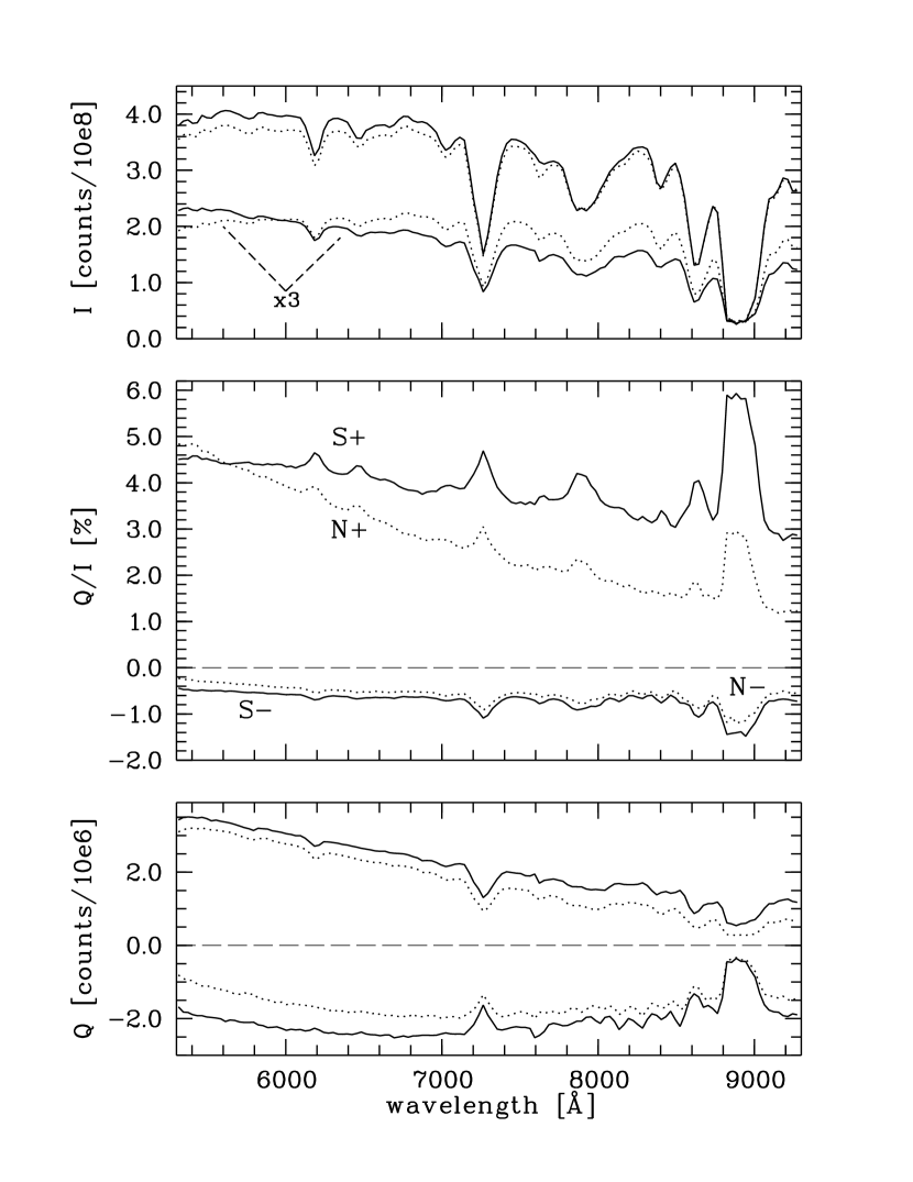
Figure 4: Spectropolarimetry of Jupiter for the S+, S$-$ (solid lines) and the N$-$ and N+ (dashed lines) regions as defined in Fig. 3. The intensity $I(\lambda)$ for the polar region S$+$ and N$+$ are multiplied by a factor of 3 with respect to S$-$ and N$-$ for visibility reasons. The middle panel gives $Q_{r}/I(\lambda)$ and the bottom panel the polarization flux $Q_{r}$.

3.3.1 Spectropolarimetry for the “extreme” polar limbs

The S+ and N+ spectropolarimetry provides only a very coarse characterization of the “average” limb polarization. For this reason we explore in this section the spectropolarimetric signal at the “extreme” polar limbs, where we find the maximum of the fractional polarization $Q_{r}/I$. We select a small spatial bin from $\pm 16^{\prime\prime}$ to $\pm 17^{\prime\prime}$, corresponding to planetographic latitudes from about $\pm 73^{\circ}$ out to the polar limbs (see Fig. 5).

For the South pole the fractional polarization reaches $Q_{r}/I=9.6~{}\%$ for the continuum in the 5300 to 6100 Å region and even 10.0 % in the $\lambda$6190 CH₄-band. Previous studies report maximum fractional polarizations of not more than $Q_{r}/I=7-8~{}\%$, most likely because the spatial resolution was worse than the $1^{\prime\prime}$ achieved with our observations. This illustrates the problem of the spatial averaging. The overall spectral slope of the fractional polarization spectra $Q_{r}/I(\lambda)$ at the extreme polar limb is flatter for the South than for the North, similar to the S+ and N+ regions. Interestingly the polarization enhancement in the strong methane bands is much less pronounced in the extreme polar limb data.

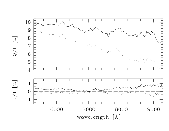
Figure 5: Fractional polarization spectra $Q_{r}/I$ and $U_{r}/I$ for the “extreme” southern (solid) and the northern (dashed) limb.

3.3.2 Spectropolarimetric signal at the equatorial limb

The spectropolarimetric observations of Jupiter taken with a slit in East-West direction cover the regions from the eastern limb at $-18.0^{\prime\prime}$ to $-12.8^{\prime\prime}$ and from $+10.7^{\prime\prime}$ to the western limb at $+18.0^{\prime\prime}$ (Fig. 1).

For both limbs the fractional polarization spectra show a positive polarization $Q_{r}/I\approx 0.5~{}\%$ for the shortest wavelengths, and $Q_{r}/I\approx 0.0~{}\%\pm 0.2\%$ for $\lambda>7000$ Å, except for the strong CH₄ band at 8870 Å, where the polarization is approximately $Q_{r}/I\approx+0.4$ %.

The spatial profiles show a general radial decrease in the fractional polarization from slightly positive values, $Q_{r}/I\approx+0.5~{}\%$ to $0.0~{}\%$, at the inner edges of the slitlets (at $-12.8^{\prime\prime}$ and $+10.7^{\prime\prime}$) towards zero or slightly negative values, $Q_{r}/I\approx 0.0~{}\%$ to $-0.5~{}\%$, further out at the eastern limb and out to $+16^{\prime\prime}$ on the western side. For a given distance from the center, the polarization is slightly more negative ($\Delta p\approx-0.2~{}\%$) on the eastern side.

This behavior is qualitatively in agreement with the E-W polarization profile derived for the ZIMPOL polarimetry for March 2003. The E-W asymmetry is switched most likely because the bright limb and terminator have switched sides between March 2003 and Nov. 2003. Also the small change in the overall polarization level for the phase angle $\alpha=6.9^{\circ}$ in March 2003 (less E-W polarization in the equator region) and $\alpha=10.4^{\circ}$ in Nov 2003 (more E-W polarization) is similar to previous studies (e.g. Morozhenko, 1973).

4 Saturn

4.1 Imaging polarimetry

The appearance of Saturn depends strongly on the inclination of the planet and its ring system. In 2003 the inclination of the polar axis with respect to the celestial plane was $27^{\circ}$, close to the maximum inclination possible for Earth-bound observations. An EFOSC2 acquisition image shows Saturn for the November 2003 run (Fig. 6). For this inclination the South pole is well visible about $1^{\prime\prime}$ inward from the limb (see Table 1). The equator is almost half way between disk center and northern limb while the ring system covers the latitudes northward of $+20^{\circ}$.

Figure 7 shows a Stokes $Q$-polarization flux image in the 7300 Å filter taken with ZIMPOL in March 2003. One can recognize the negative (E-W) polarization of the ring, a weak positive feature at the southern pole, a polarization flux close to zero in the south, corresponding to latitudes around $-60^{\circ}$, and a dominant strong positive feature at the equator.

The $U$-image corresponding to Fig. 7 shows near the southern limb negative $U/I\approx-0.3$ % and positive $\approx+0.3$ % features on the east and west sides of the South pole, respectively very much like the $U$-pattern for the poles of Jupiter. This indicates that the polarization features at the South pole have a radial polarization direction. For the rings of Saturn there is essentially no $U$-signal visible.

The equatorial polarization reaches in the 7300 Å filter a maximum fractional polarization of $Q/I\approx+1.6$ % and extends about 4^′′ to 5^′′ in east-west direction. This equatorial feature is remarkable since it was not present in early measurements (e.g. Hall and Riley, 1974; Dollfus, 1996). A similar signal is also present in the 6010 Å imaging polarimetry from the same date and in the 5500 Å, 6010 Å, and 7300 Å  filter ZIMPOL polarimetry from March 2002 (Gisler et al., 2003). Also our spectropolarimetric observations of November 2003 confirms the presence of this transient signal.

The $U$-signal at the equator is weak with a fractional polarization of $U/I\approx-0.3$ % at the east limb, $-0.1$ % at the meridian, and about $+0.1$ % on the west limb. These are only small signals when compared to the fractional $Q/I$-polarization of $\approx+1.5$ % at the intersection of meridian and equator. This indicates that the equatorial polarization extends from about $-30^{\circ}$ to $+30^{\circ}$ in longitude along the equatorial band and has a predominant orientation in north-south direction.

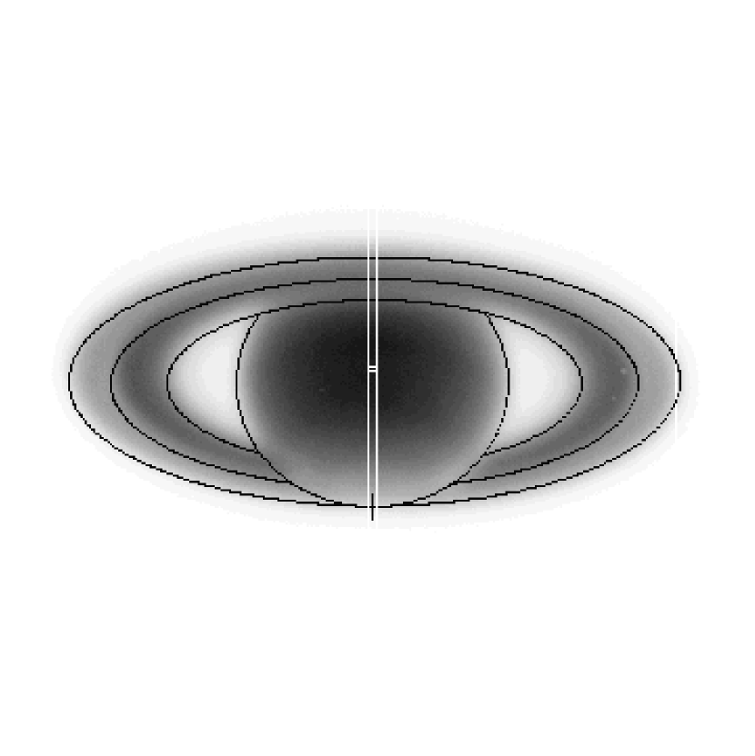
Figure 6: EFOSC2 acquisition image of Saturn taken on Nov. 30, 2003. North is up and East is to the left. The limb of the planetary disk, as well as the position of the south pole and the limits of the A and B rings are indicated. In addition, the two slit positions for spectropolarimetry are marked with white rectangles which overlap at the center.

Figure 7: ZIMPOL Stokes $Q$-flux image of Saturn, obtained in the methane 730 nm filter. In the south the planet occults the ring, except for a small rim with a width of about $1.5^{\prime\prime}$.

4.2 Profiles for the planet and the ring

4.2.1 Comparison of North-South and East-West profiles

Figure 8 shows the North-South and East-West profiles extracted for the 7300 Å CH₄ filter ZIMPOL observations of March 2003. The middle panel shows the fractional radial polarization $Q_{r}/I$. The N-S profile for $Q_{r}/I$ is positive everywhere on the planetary disk and negative for the ring. There are two peaks, one of $Q_{r}/I\approx+1.0~{}\%$ at the southern pole (at approximately $-8.5^{\prime\prime}$) and a stronger peak of $Q_{r}/I\approx+1.6~{}\%$ at the equator ($+4^{\prime\prime}$) coincident with the intensity maximum. For the E-W direction the radial polarization is positive for the ring (parallel to the slit) and negative for the planet. The strongly negative $Q_{r}/I$ polarization between planet and ring is probably a spurious effect because in these gaps the photon statistics is low and the impact of scattered light, and residual systematic noise effects are large. The polarization flux profile $Q_{r}$ shows that the equatorial polarization feature is really strong.

As described in Sect. 2.2 the calibration for the ZIMPOL-polarimetry is based on the assumption that the fractional $Q/I$-polarization is $-0.4~{}\%$ for the ring. The good agreement between the ZIMPOL and EFOSC2 data support this calibration procedure.

Figure 8: Saturn N-S (full line) and E-W profiles (dotted line) for the intensity (top), the fractional radial polarization $Q_{r}/I$, and the $Q_{r}$ polarization flux for the wavelength $\lambda$7300Å.

4.2.2 Polarization measurements for the central meridian

Figure 9 compares the meridional profiles for the strong methane band $\lambda$8870 and the continuum at $\lambda$6000. For the $\lambda$8870 CH₄ band the fractional polarization $Q_{r}/I$ is positive for the southern latitudes and negative at the equator and the ring. It appears that $Q_{r}/I$ has a maximum at the southern pole at about $-7.5^{\prime\prime}$. The polarization flux $Q_{r}$ for $\lambda$8870 illustrates the weakness of the polarization signal at this wavelength. In $Q_{r}$ no polarization flux maximum is visible at the south pole. Interestingly there is a small negative polarization for the CH₄ wavelength near the equator in contrast to the strong positive polarization signal at shorter wavelengths.

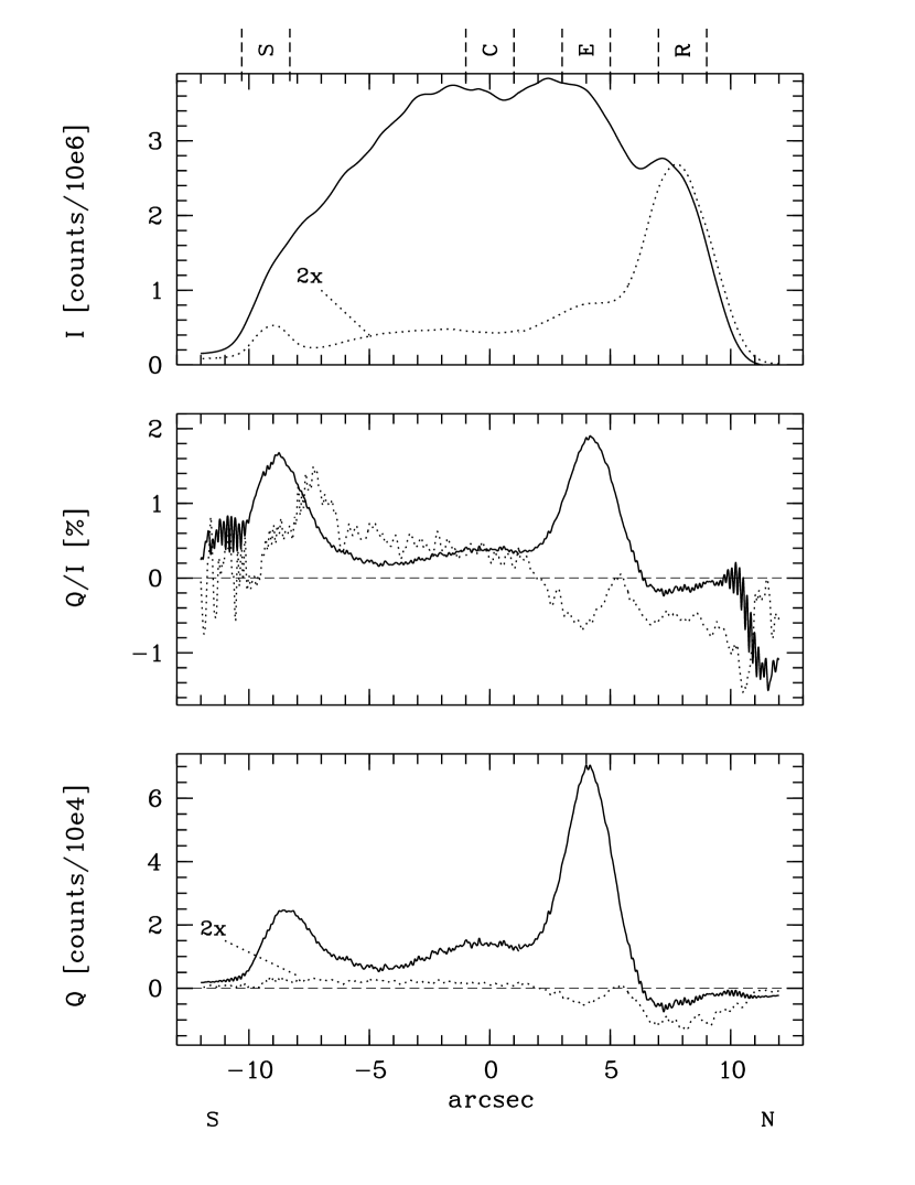
Figure 9: Polarimetric profiles of Saturn along the central meridian for the continuum wavelength region 6000 Å (full line) and the deep methane absorption band at 8870 Å (dotted line).

We select four regions along the the central meridian with a width of $2^{\prime\prime}$ as indicated in Fig. 9. These regions are “S” for southern limb, “C” for the center of the disk, “E” for the equator, and “R” for the ring and their relative intensity and fractional polarization are given in Table 3.

For the interpretation of the polarization in Table 3 the orientation of the scattering plane has to be taken into account. For the November 2003 observations the scattering plane is tilted by $+12^{\circ}$ with respect to the E-W direction of Saturn. Therefore a scattering polarization perpendicular to the scattering plane produces besides a $Q$-signal also an $U$ signal at the level of $U=0.45\,Q$. For example, the $\lambda$6000 polarization for the “S” region has an orientation of $\theta_{p}=+5^{\circ}$, compatible with $\theta_{p}=0^{\circ}$ for a polarization in N-S direction (or radial), while the strong polarization in the equatorial region “E” has an orientation of $\theta_{p}=+11^{\circ}$, perpendicular to $\theta=102^{\circ}$ of the scattering plane.

For the polarization of the E and W cusps of the ring the literature gives values of $\approx-0.4~{}\%$ parallel to the scattering plane for phase angles near $4^{\circ}$ (e.g. Dollfus, 1979, 1996; Johnson et al., 1980). For the ring “R” we measure for $\lambda$6000 and $\lambda$8100 a $Q/I$ polarization component between $-0.1~{}\%$ and $-0.2~{}\%$, or a polarization which is lower (less negative) by about 0.2 % than expected. This effect has been previously described by Kemp and Murphy (1973), and at that time it was explained by an admixture of $+Q/I$-polarized light from Saturn transmitted through the ring. Since we know now that the optical depth of the ring is rather high, we attribute this decrease in polarization to light from the adjacent equatorial region scattered by the instrument. In the dark CH₄ band the reflection from the planet is strongly reduced, so that the ring polarization is less diluted by scattered light from the planet.

The uncertainties for the fractional polarization due to instrument calibration and slit positioning errors are about $\Delta Q_{r}/I,\Delta U_{r}/I\approx\pm 0.2~{}\%$. Photon noise errors are negligible compared to calibration errors and unidentified instrumental effects.

Table 3: Relative intensity $I/I_{\rm slit}$, reflectivity $f$, and fractional radial polarization $Q_{r}/I$ and $U_{r}/I$ for Saturn for the four $2^{\prime\prime}$ wide regions S, C, E, R on the central meridian and the entire meridian. The first row gives the center of these meridional sections and the second row the corresponding planetographic latitude.

	S	C	E	R	total slit
location
$x_{\rm cent}$	$-9.3^{\prime\prime}$	$0.0^{\prime\prime}$	$+4.0^{\prime\prime}$	$+8.0^{\prime\prime}$
latitude	$-65^{\circ}(^{a})$	$-30^{\circ}$	$0^{\circ}$	$+30^{\circ}$
continuum 5900-6100 Å, $A_{g}=0.54$
$I/I_{\rm slit}$	0.037	0.124	0.129	0.084	1.000
$f$		0.68	0.71	0.46
$Q_{r}/I$ [%]	$+1.40$	$+0.34$	$+1.65$	$-0.10$	$+0.54$
$U_{r}/I$ [%]	$+0.24$	$+0.08$	$+0.68$	$-0.17$	$+0.16$
continuum 8100-8300 Å, $A_{g}=0.56$
$I/I_{\rm slit}$	0.027	0.125	0.130	0.088	1.000
$f$		0.71	0.74	0.50
$Q_{r}/I$ [%]	$+0.40$	$+0.16$	$+0.02$	$-0.21$	$+0.05$
$U_{r}/I$ [%]	$+0.15$	$+0.02$	$-0.22$	$-0.16$	$-0.05$
CH4 8800-8940 Å, $A_{g}=0.07$
$I/I_{\rm slit}$	0.045	0.047	0.102	0.301	1.000
$f$		0.09	0.20	0.6
$Q_{r}/I$ [%]	$+0.27$	$+0.19$	$-0.35$	$-0.40$	$-0.18$
$U_{r}/I$ [%]	$+0.36$	$-0.04$	$-0.74$	$-0.50$	$-0.38$

$a$: southern limb beyond the south pole at longitude $+180^{\circ}$ from the central meridian

Our relative $I/I_{\rm slit}$ for Saturn can be converted into reflectivities $f_{\lambda}$ using the HST observations from December 2002, published by Perez-Hoyos et al. (2005). From the electronic figure we obtain $f_{6750}=0.72\pm 0.01$ for the sub-Earth point “C”. Temporal changes in $f_{\lambda}$ for Saturn can be significant, due to the strong inclination of the planet and the variable shadowing by the ring system. But the data from December 2002 are useful for us because no strong reflectivity changes were noticed between Dec. 2002 and Aug. 2003 (Perez-Hoyos et al., 2005) and between March 2003 and March 2004 (Karkoschka and Tomasko, 2005).

Reflectivities for other wavelengths are deduced with the global albedo spectrum of Karkoschka (1998), according to $f_{\lambda}=f_{6750}\,A_{g}(\lambda)/A_{g}(6750)$, using $A_{g}(6750)=0.57$. The reflectivities for the slit sections S, E, and R scale like the $I/I_{\rm slit}$ values (Table 3).

4.2.3 Spectropolarimetry for Saturn

The spectropolarimetric signal for the southern limb (S), disk center (C), equator (E), and the ring (R) are plotted in Fig. 10. The spectra are averages for $2^{\prime\prime}$ wide spatial regions as indicated in Fig. 9.

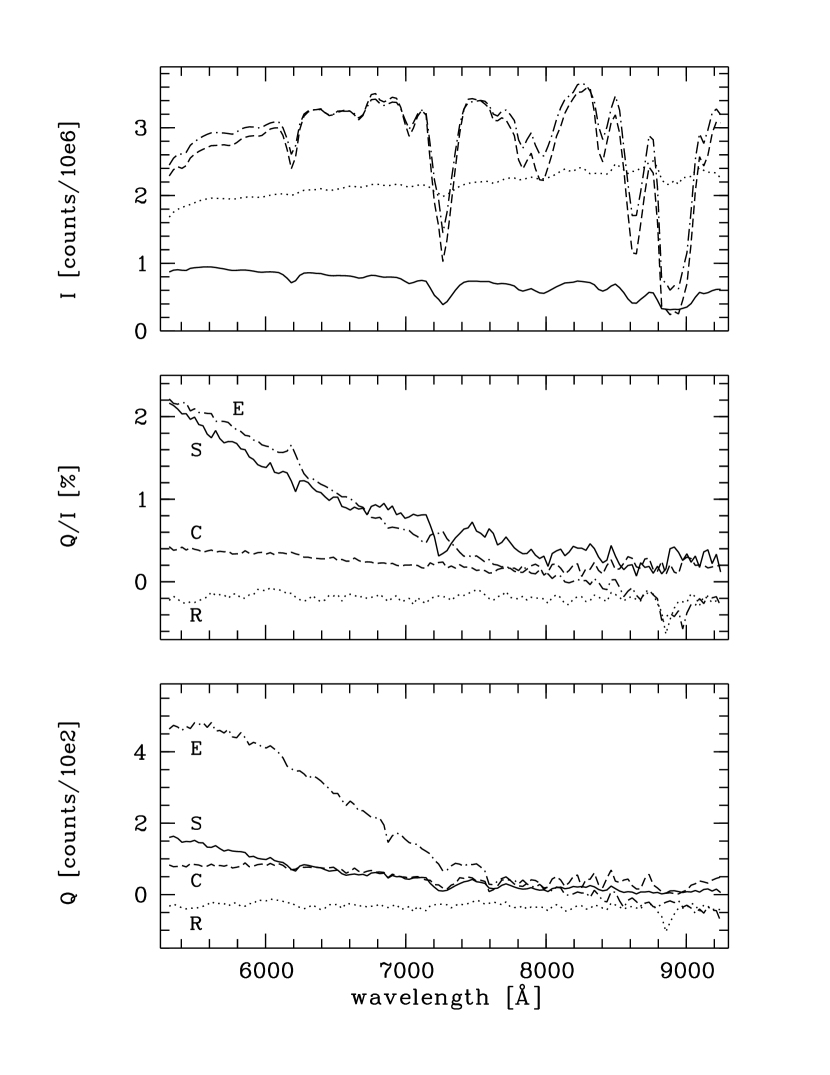
Figure 10: Spectropolarimetry for the four regions of Saturn: south pole (solid line), center (dashed line), equator (dot-dashed line), and ring (dotted line). Top panel: intensity spectra $I(\lambda)$ (counts). Middle panel: fractional polarization $Q_{r}/I(\lambda)$. Positive is parallel to the slit and negative is perpendicular. Bottom panel: polarized flux $Q_{r}(\lambda)$.

The intensity spectra S, C, and E from the planetary disk show all the well known CH₄-bands. The ring spectrum R is essentially featureless apart from very weak features at the wavelength of strong CH₄ bands, which can be attributed to scattered light from the adjacent planetary disk.

A strong fractional polarization ($Q_{r}/I>1~{}\%$) is present at the south pole, “S”, and equator, “E”, respectively. $Q_{r}/I$ decreases steeply towards longer wavelengths from about $Q_{r}/I\approx+2.2~{}\%$ at 5300 Å to about $+0.2~{}\%$ at 8000 Å, and is close to zero for longer wavelengths. The fast drop in polarization in $Q_{r}/I$ or in the polarization flux $Q_{r}$ with wavelength is typical for a Rayleigh scattering layer above a weakly or non-polarizing cloud surface (e.g. Buenzli and Schmid, 2009).

$Q_{r}/I$ for the disk center is low, only $+0.4~{}\%$ at 5300 Å, and it decreases steadily towards zero. It is not clear, whether the negative feature in the CH₄-band at $\lambda$8870 is real or just a spurious effect. As shown in previous studies (e.g. Kemp and Murphy, 1973; Dollfus, 1996) the fractional polarization of the ring depends only little on wavelength. A weak feature is visible in the strong CH₄-band $\lambda$8870, which could be due to enhanced contamination from scattered light.

For the “E” and “S” regions there are essentially no narrow spectral features visible in $Q_{r}/I$. In particular there is no clear enhancement in strong methane bands like $\lambda$7270 or $\lambda$8870, as observed for Jupiter (see Sect. 3.3), or Uranus and Neptune (Joos and Schmid, 2007a).

5 Investigation of the strongest polarization features

Our polarimetry of Jupiter and Saturn has revealed two surprising polarization features: a very high limb polarization reaching a maximum of more than 9 % between 5300 Å and 6500 Å for the South pole of Jupiter, and a strong equatorial polarization for Saturn. We explore whether these observational results are compatible with simple scattering models.

For a detailed characterization of the scattering particles in Jupiter and Saturn extensive modelling would be required. Unfortunately there exist up to now only few limb polarization models – essentially only the grid for Rayleigh scattering atmospheres by Buenzli and Schmid (2009) and a few previous, mostly analytic results as summarized in Schmid et al. (2006a). Therefore it is not well explored yet how the limb polarization depends on the scattering phase matrix of the haze particles, the stratification of the atmosphere, and the optical depth of absorbers. Therefore, our model fitting remains ambiguous without extensive model simulations which are beyond the scope of this paper.

5.1 Polarization model for the poles of Jupiter

Model calculations for Jupiter were carried out in order to explain the observed peak limb polarization of more than 9 % in R-band and more than 9.5 % in the V-band at the South pole. Considering that the seeing degrades this polarization, the maximum limb polarization must be well above 10 %. Rayleigh scattering models yield up to 10 % limb polarization (e.g. Schmid et al., 2006a) but only for highly absorbing atmosphere models, which are not appropriate for the reflected intensity seen on the poles of Jupiter.

Detailed scattering models for the polarization of Jupiter were presented by Smith and Tomasko (1984) and Braak et al. (2002), but only for mid and low latitudes. No detailed scattering models exist for the polarization at the poles. Smith and Tomasko (1984) made a simple fit to the polarization measured in the red with the Pioneer spacecraft for a Rayleigh scattering layer with single-scattering albedo of $\omega=0.983$, optical thickness $\tau=0.5$, and a surface albedo of $A_{S}=0.67$. However, this Rayleigh scattering model yields a maximum limb polarization of only 7.3 %, or $\approx 6.5~{}\%$ if the degradation by the seeing is considered, whereas our measurements show a much higher fractional polarization.

We calculate the polarization along the central meridian of Jupiter, considering three zones: the polar S+ and N+ zones, and a central zone, corresponding roughly to the S$-$, N$-$, and center regions in Table 2.

For the S+ and N+ zones we use the Monte Carlo multiple scattering code described in Buenzli and Schmid (2009). The chosen atmosphere structure is very similar to the haze model presented by Smith and Tomasko (1984) for low latitudes. They determined haze and gas properties for the South Tropical Zone and South Equatorial Band with an atmosphere consisting of a top gas layer G1, a scattering haze layer H, a lower gas layer G2, and an optically thick surface layer S at the bottom. We fit the polar regions S+ and N+ with this model. For the wavelength 6000 Å the optical depths for the two gas layers are $\tau_{\rm G1}=0.011$ and $\tau_{\rm G2}=0.018$, and the single scattering albedo is $\omega_{\rm G}=0.976$, calculated for a methane abundance of 0.18 %. Thus, the haze layer is geometrically thin and located at a pressure level of 290 mbar, while the opaque surface layer is at 760 mbar. The continuum polarization at 6000 Å does not depend much on the exact height of the haze and cloud surface layers and e.g. 40 mbar or 1200 mbar, respectively, would not notably change the intensity and polarization. The situation is different for the polarization in the CH₄ bands which depends in various ways on the pressure level of the different layers.

The free parameters of our model are: the albedo cloud layer $A_{\rm S}$ assumed to be a grey Lambert surface, the optical thickness of the haze layer $\tau_{\rm h}$, and the haze parameters, which are single scattering albedo $\omega_{\rm h}$, single term Henyey-Greenstein asymmetry parameter $g_{\rm h}$, and maximum polarization for right angle scattering $p_{\rm h}$ (see Braak et al., 2002). The polar model is independent of latitude, but the incidence and viewing angles produce a latitude dependence in the reflected polarization and intensity.

For the reflected intensity at lower latitudes the same model is used, but for the fractional polarization an “artificial” constant value of $Q_{r}/I=-0.7~{}\%$ is adopted. The negative polarization is introduced to fit the transition between the positively polarized polar zones and the negative central zone. The borders $r_{\rm S}$ and $r_{\rm N}$ are free parameters which are determined in the data fitting process.

In order to describe the smearing of the signal due to atmospheric seeing and instrumental light scattering, the “discrete” three zone model is convolved with a Moffat (Moffat, 1969) point spread function (PSF). In the formalism of Trujillo et al. (2001) this PSF includes a $\beta$-parameter which describes the scattering wing. A small $\beta$ implies strong wings, a Gaussian is obtained for $\beta\rightarrow\infty$, while atmospheric turbulence theory predicts $\beta=4.76$. For our observations we derive $\beta=1$ from the residual light outside the nominal limb, indicating significant scattering in the instrument.

In Fig. 11 the observed intensity and polarization profiles for the central meridian for 6000 Å are compared with the model fit. At the poles $|r|>0.8$ the match is satisfactory except for the fractional polarization outside the limb $|r|>1$, where the statistical errors are large because $I\rightarrow 0$. At low latitudes there are some discrepancies because we did not try to fit the band structure for the intensity, and we adopted a constant value for the fractional polarization.

A good fit for the limb polarization at $\lambda=6000$ Å for both poles is obtained for strongly polarizing $p_{\rm h}=1$ haze with a low absorption $\omega_{\rm h}=0.99$ and asymmetry parameter $g_{\rm h}=0.6$. Such scattering parameters are typical for aggregate particles as proposed to be present in Jupiter and Titan by West and Smith (1991). Small Mie scatterers with diameters much smaller than the wavelength of the scattered light have similar scattering parameters. But the scattering cross section for small spheres is much higher in the blue and one would expect a fractional limb polarization which decreases rapidly with wavelength (as seen for the pole and the equator of Saturn). The scattering cross section and therefore the scattering optical depths of the haze layer are expected to decrease only slowly with wavelength for aggregate particles and they can therefore explain the rather gentle decrease in the $Q/I$ and $Q$-spectra towards longer wavelengths observed for the poles of Jupiter (see Fig. 4).

The measured limb polarization at the poles for $r=\pm 0.96$ is about 9.8 % in the South and 8.4 % in the North. The North-South differences can be explained by different optical depths $\tau_{\rm h}(N+)=0.72$, $\tau_{\rm h}(S+)=1.1$ for the haze layers.

Our model fit includes the smearing due to seeing and the modelling indicates that the intrinsic limb polarization reaches maxima of about 11.5 % in the South and 10.0 % in the North. Such a high limb polarization is probably only possible with particles having a scattering phase function with reduced backscattering, with an asymmetry parameter comparable to $g\approx 0.6$ as used in our model.

Figure 11: Comparison of the model fit (dashed line) with the observed 6000 Å N-S profile (dotted line) of Jupiter.

Our model fit is not unique. However, many parameters are already well constrained. From the parameter space explored by us it seems very likely that the asymmetry parameter lies in the range $0.8<g_{\rm h}<0.5$ and the single scattering polarization is $p_{\rm h}>0.8$.

The locations of the transitions $r_{\rm S}$ and $r_{\rm N}$ between the highly polarized poles and the negatively polarized central zone are at $r=\pm 0.82\pm 0.01$, identical for both hemispheres. This correspond to a planetographic latitude of $\pm 58^{\circ}\pm 3^{\circ}$. In the South the transition between the S+ and the central region is compatible with an unresolved discontinuity. In the North the transition is more gradual, with a weak wing of positive polarization towards lower latitude. This is in qualitative agreement with Fig. 14 in Smith and Tomasko (1984), who measured the latitudinal polarization dependence with Pioneer for large phase angles (82^∘ and $98^{\circ}$). Their red filter data show a steep increase in the polarization in the South from about 10 % at a latitude of $-55^{\circ}$ to about 33 % at $-65^{\circ}$ and a more gradual increase from 13 % at $+55^{\circ}$ to about 25 % at $+65^{\circ}$ in the North.

The surface albedo $A_{S}=0.75$ is also quite well constrained, since a high value $A_{S}>0.9$ would significantly reduce the resulting fractional polarization and a low value $A_{S}<0.6$ would underpredict the reflectivity at the poles. It also seems quite safe to explain the North-South asymmetry in the polar polarization with a difference in the optical thickness of the polarizing haze layer.

Finally, it is interesting to note that the haze model for low latitudes with $\omega_{h}=0.95$, $p_{\rm h}=0.9$ and $g_{h}=0.75$ from Smith and Tomasko (1984), which was also adopted by Braak et al. (2002), cannot fit the polarization at the poles. This points to distinct differences between the haze particles at the poles and at lower latitudes.

5.2 The transient polarization feature at the equator of Saturn

For Saturn we investigate the nature of the surprisingly strong transient polarization feature at the equator $Q_{r}/I(6000~{}{\rm\AA})=+1.65~{}\%$ (Table 3), present in our 2003 (and 2002) data. The transient nature of the feature could be related to the high inclination of $\approx 26^{\circ}$ of the Saturn system during our observations. In the following we explore possible explanations for this feature.

At exact opposition no polarization signal is expected from the center of the planetary disk for symmetry reasons. Our spectropolarimetric observations were taken at phase angle $\alpha=3.7^{\circ}$. The equatorial polarization cannot be ascribed to a phase effect because for this phase one expects only a negligible positive polarization for small, positive polarizing scattering particles, or a small $Q/I\approx-0.2~{}\%$ negative polarization for e.g. large negatively polarizing scattering particles.

Higher order scatterings produce a radial limb polarization, but this initially increases only slowly when going from the center of the disk towards the limb. A semi-infinite, conservative ($\omega=1$) Rayleigh scattering atmosphere produces a fractional limb polarization of only $Q_{r}/I=+1.3~{}\%$ at $r/r_{\rm limb}\approx 0.5$ or $\theta\approx 30^{\circ}$ (e.g. Buenzli and Schmid, 2009; Schmid et al., 2006a) which is roughly the location of the equator in our observations. A slightly higher limb polarization is possible with a stratospheric haze model similar to the one determined by Karkoschka and Tomasko (2005) consisting of a relative thick layer with high albedo, highly polarizing, and forward scattering particles

However, the interpretation of the strong equatorial polarization in Saturn as higher order scattering or “limb polarization” effect is in contradiction with the observations. Limb polarization would produce a $Q_{r}/I$ signal along the entire equatorial band with maxima above 5 % at the equatorial limbs. This is not observed. In addition we would expect a high polarization of at least $p>20$ % at large phase angles which is also not visible in the contemporaneous Cassini polarization image of West et al. (2009).

An alternative explanation could be strong light scattering from the inclined ring system. But this can be rejected with an order of magnitude estimate. The solid angle subtended by the illuminated ring system as seen by the equatorial region is small and the forward scattering of light by the ring is inefficient because the ring is made of large ($>1$ mm), back-scattering bodies. For example Dones et al. (1993) show that the phase function for forward scattering by the ring is only $I(\alpha)<0.1\,I(0)$ for $\alpha>135^{\circ}$. Therefore the irradiation with light scattered from the rings is well below 1 % of the direct irradiation from the sun and it is impossible that this low level of indirect light produces a significant fractional polarization at the equator.

Which other effect could explain the transient equatorial polarization of Saturn if phase effects, limb polarization, and ring reflection can be discarded? The unknown effect seems to be restricted to the equatorial band and photon incidence and emergence angles of $\approx 25^{\circ}$ for the incoming and back-scattered radiation. Such a localized feature could perhaps be formed by a higher order scattering effect in an optically thick, but geometrically thin cloud or aerosol layer. We are not aware of investigations of such scattering geometries. However, we may hope that a detailed analysis of the Cassini polarimetry presented in West et al. (2009) clarifies the case.

6 Summary, discussion, and conclusions

This work presents ground-based spectropolarimetry and imaging polarimetry of Jupiter and Saturn. The new data are of unprecedented quality because modern instruments with CCD detectors were used. This type of data opens up many new avenues of polarimetric investigation for planets, because the polarization signal can be quantified much more accurately from imaging polarimetry and spectropolarimetry, when compared to previous aperture polarimetry. Well calibrated data with quantified seeing effects allow for detailed comparisons with model calculations of the scattering layers in Jupiter and Saturn.

There are a series of important results in this work:

We present for the first time spectropolarimetry for the strongly polarized poles of Jupiter. The polarization shows an overall decrease with wavelength and a rich spectral structure with enhanced fractional polarization in strong methane absorptions. In the polarization flux spectrum the absorption bands are still visible as absorptions, although with a lower equivalent width than in the intensity spectrum. The enhancement in fractional polarization $Q/I$ in the methane bands can be explained by a highly polarizing stratospheric haze layer above an atmosphere where multiple scatterings (or the reflection of unpolarized light) are suppressed in the methane absorptions.

The fractional polarization at lower latitudes of Jupiter is small and slightly negative with an enhanced polarization signal in strong methane absorption.

From the polarization profiles along the central meridian of Jupiter we can derive a latitude of $\pm 58^{\circ}$ for the transition between the polar region with strong positive polarization and lower latitudes with a negative polarization. Our results agree very well with the polarization measurements from the Pioneer missions (Smith and Tomasko, 1984). Stratospheric haze is responsible for the strong polar polarization and the sharp transition is pointing to a well defined border in the stratospheric circulation.

For the poles of Jupiter we measure in the V-band a seeing limited peak limb polarization of $+9$ to $+10~{}\%$. This indicates a resolution-corrected peak polarization of about $+11.5~{}\%$. All previous studies reported lower values ($p\approx 6-8$ %) for the maximum polarization at the poles of Jupiter. This difference can be explained by the better spatial resolution (seeing $\approx 1^{\prime\prime}$) of our data and the appropriate seeing correction.

We derive the polarization flux of the entire positively polarized polar hoods (called $S+$ and $N+$ in this work). This approach should allow an easy comparison of our data with previous and future observations for long term studies which are interesting for investigations of the haze production, destruction and transport in the polar stratosphere of Jupiter. Such long term polarization changes were reported e.g. by Starodubtseva et al. (2002) and Starodubtseva (2009).

We found no limb polarization models with a limb polarization higher than 10 % in the literature. For this reason we carried out exploratory calculations. They indicate that a polar haze layer consisting of forward scattering and highly polarizing aggregate particles as proposed by West and Smith (1991) is compatible with our observations.

The polarization of Saturn is lower than that of Jupiter. Our observations of 2002 and 2003 revealed at 6000 Å a positive feature (about $1.4~{}\%$) at the South pole and a stronger ($>1.6~{}\%$) transient polarization feature near the equator.

Spectropolarimetrically, Saturn shows hardly any enhancements in the fractional polarization at wavelengths of strong methane bands in strong contrast to the case of Jupiter. This indicates that the polarizing particles in Saturn are not located in a discrete layer, but well distributed in the scattering atmosphere. Absorptions within the polarizing scattering layer reduce the reflected intensity $I$ and polarization flux $Q$ simultaneously and causes therefore no or only weak features in the fractional polarization spectrum $Q/I$.

At the South pole and the equator the polarization decreases rapidly with wavelength, and essentially no polarization $p<0.4~{}\%$ is present for wavelengths above $7500$ Å. The fast decrease of the limb polarization with wavelength is indicative for small scattering particles ($<100$ nm) as proposed by Karkoschka and Tomasko (2005) based on HST imaging.

The strong equatorial polarization feature in Saturn is remarkable since it was not present in earlier measurements. During our observations the inclination of Saturn was high and therefore the effect could be seasonal. We investigated various possibilities to explain the equatorial polarization but could not find a reasonable solution. Despite this we are certain that the observed fractional polarization of about $p=1.6~{}\%$ in polar direction is real. It seems interesting to investigate this feature further with other data or model simulations.

An important conclusion from this paper is that modern polarimetric measurements of Jupiter and Saturn from the ground can provide accurate quantitative results which constrain strongly the scattering properties of the atmospheres. This type of investigations certainly did not receive sufficient attention in the last decades, and more observations, e.g. for other wavelengths, and a lot of limb polarization modelling still needs to be done. A first step with model simulations was done by Buenzli and Schmid (2009) who present an extensive grid of model calculations for Rayleigh scattering atmospheres. Further models ought now to be calculated which should investigate the dependence of the limb polarization signal on the scattering phase matrix of different populations of haze particles. In additions one needs to take into account the spectropolarimetric structure in the methane bands in order to derive the vertical stratification of the scattering layers.

Scattering layers, reflecting the solar light, are an intriguing aspect of solar system planets. They affect the radiative transfer in these objects. For the investigation of the reflected light from extra-solar planets a comprehensive understanding of the physics of the high altitude haze layers is very important. For this reason it is essential to carry out detailed investigations of the reflecting layers in solar system planets. Investigations based on modern polarimetric observations, as presented in this work for Jupiter and Saturn, are therefore very valuable for progress in this direction.

Acknowledgements: We are indebted to the ESO La Silla support team at the 3.6m telescope who were most helpful with our very special EFOSC2 instrument setup. We are particularly grateful to Oliver Hainaut. We thank Harry Nussbaumer for carefully reading the manuscript. We also acknowledge the many useful comments from the referees. This work was supported by a grant from the Swiss National Science Foundation.

References

- The Astronomical Almanach (2003) The Astronomical Almanach, 2003, US Gov. Printing Office Washington, The Stationary Office, London
- Braak et al. (2002) Braak, C. J., de Haan, J. F., Hovenier, J. W., Travis, L. D. 2002. Galileo Photopolarimetry of Jupiter at 678.5 nm. Icarus 157, 401-418.
- Buenzli and Schmid (2009) Buenzli, E., Schmid, H.M., 2009. A grid of polarization models for Rayleigh scattering planetary atmospheres. A&A 504, 259-276
- Carlson and Lutz (1989) Carlson, B.E., Lutz, B.L., 1989. Spatial and temporal variations in the atmosphere of Jupiter: polarimetric and photometric constraints. In: Belton, M.J.S., West, R.A., Rahe, J., Proc. of Workshop on Time-variable phenomena in the Jovian System, NASA special publication series, NASA-SP-494, pp. 289-298
- Chanover et al. (1996) Chanover, N.J., Kuehn, D.M., Banfield, D., Momary, T., Beebe, R.F., Baines, K.H., Nicholson, P.D., Simon, A.A., Murrell, A.S., 1996. Absolute Reflectivity Spectra of Jupiter: 0.25-3.5 Micrometers. Icarus 121, 351-360.
- Cochran et al. (1981) Cochran, A.L., Trafton, L.M., Cochran, W.D., Barker, E.S., 1981. Spectrometry of Jupiter at selected locations on the disk during the 1979 apparition. AJ 86, 1101-1107.
- Coffeen (1979) Coffeen, D.L., 1979. Polarization and scattering characteristics in the atmospheres of Earth, Venus, and Jupiter. J. Opt. Soc. Am. 69, 1091
- Dollfus (1957) Dollfus, A., 1957. Étude des planètes par la polarisation de leur lumière. Suppl. Ann. Astrophys. 4, 3-114,
- Dollfus (1979) Dollfus, A., 1979. Optical reflectance polarimetry of Saturn globe and rings. I - Measurements on B ring. Icarus 37, 404-419.
- Dollfus (1996) Dollfus, A., 1996. Saturn’s Rings: Optical Reflectance Polarimetry. Icarus 124, 237-261.
- Dones et al. (1993) Dones, L., Cuzzi, J. N., Showalter, M. R. 1993. Voyager Photometry of Saturn’s A Ring. Icarus 105, 184-215.
- Gehrels et al. (1969) Gehrels, T., Herman, B. M., Owen, T., 1969. Wavelength Dependence of Polarization. XIV. Atmosphere of Jupiter. Astron. J. 74, 190-199.
- Gisler et al. (2003) Gisler, D., Schmid, H.M., 2003. Non-solar Applications with the ZIMPOL Polarimeter. In: Trujillo Bueno, J., Sanchez Almeida, J. (Eds.), Conference on Solar Polarization, September 30 - October 4 2002, Tenerife, Spain, ASP Conf. Ser. 307, 58-61.
- Gisler et al. (2004) Gisler, D., Schmid, H.M., Thalmann, C., Povel, H.P., Stenflo, J.O., Joos, F., et al., 2004. CHEOPS/ZIMPOL: a VLT instrument study for the polarimetric search of scattered light from extrasolar planets. In: Moorwood, A.F.M., Iye, M. (Eds.), SPIE conference on Ground-based instrumentation for Astronomy, Proc. SPIE Vol. 5492, 463-474.
- Hall and Riley (1968) Hall, J. S., Riley, L. A., 1968. Photoelectric observations of Mars and Jupiter with a scanning polarimeter. Lowell Obs. Bull. 7, 83-92.
- Hall and Riley (1974) Hall, J. S., Riley, L. A., 1974. A photometric study of Saturn and its rings. Icarus 23, 144-156.
- Hall and Riley (1976) Hall, J. S., Riley, L. A., 1976. A polarimetric search for fine structure on Jupiter’s disk. Icarus 29, 231-234.
- Hough et al. (2006) Hough, J.H., Lucas, P.W., Bailey, J.A., Tamura, M., Hirst, E., Harrison, D., Bartholomew-Biggs, M., 2006. PlanetPol: A Very High Sensitivity Polarimeter. PASP 118, 1302-1318.
- Johnson et al. (1980) Johnson P.E., Kemp J.C., King R., Parker T.E., Barbour M.S., 1980. New results from optical polarimetry of Saturn’s rings. Nature 28, 146-149.
- Joos and Schmid (2007a) Joos, F., Schmid, H.M., 2007a. Limb polarization of Uranus and Neptune. II. Spectropolarimetric observations. A&A 463, 1201-1210.
- Joos and Schmid (2007b) Joos, F., Schmid, H.M., 2007b. Polarimetry of Solar System Gaseous Planets. The Messenger, 130, 27-31.
- Karkoschka (1998) Karkoschka, E., 1998. Methane, Ammonia, and Temperature Measurements of the Jovian Planets and Titan from CCD-Spectrophotometry. Icarus 133, 134-146
- Karkoschka and Tomasko (2005) Karkoschka, E., Tomasko, M., 2005. Saturn’s vertical and latitudinal cloud structure 1991-2004 from HST imaging in 30 filters. Icarus 179, 195-221.
- Kattawar and Adams (1971) Kattawar, G.W., Adams, C.N., 1971. Flux and Polarization Reflected from a Rayleigh-Scattering Planetary Atmosphere. ApJ 167, 183-192.
- Kemp et al. (1971) Kemp J.C., Wolstencroft R.D., Swedlund J.B., 1971. Circular Polarization: Jupiter and Other Planets. Nature 232, 165-168.
- Kemp and Murphy (1973) Kemp, J.C., Murphy, R.E., 1973. The Linear Polarization and Transparency of Saturn’s Rings. ApJ 186, 679-686.
- Leroy (2000) Leroy, J.L., 2000. Polarization of light and astronomical observations. Chapts. 5 and 6, Gordon & Breach.
- Lyot (1929) Lyot, B., 1929. Recherches sur la polarisation de la lumière des plant̀es et de quelques substances terrestres. Ann. Observ. Meudon, VIII, 1-144. English translation, NASA TT F-187.
- Moffat (1969) Moffat, A.F.J., 1969, A Theoretical Investigation of Focal Stellar Images in the Photographic Emulsion and Application to Photographic Photometry. A&A 3, 455-461
- Moreno et al. (1991) Moreno, F., Molina, A., Lara, L.M., 1991. Charge-coupled device spectral images of spatially resolved regions of Jupiter in the 6190 and 8900 Å methane and 6450 Å ammonia bands during the 1989 opposition. Journal of Geophys. Res. 96, 14119-14127.
- Morozhenko (1973) Morozhenko, A. V., 1973. Polarimetric Observations of the Giant Planets. III. Jupiter. Soviet Astronomy, 17, 105-107.
- Ortiz et al. (1995) Ortiz, J.L., Moreno, F., Molina, A., 1995. Saturn 1991-1993: Reflectivities and limb-darkening coefficients at methane bands and nearby continua – temporal changes. Icarus 117, 328-344.
- Perez-Hoyos et al. (2005) Perez-Hoyos, S., Sanchez-Lavega, A., French, R.G., Rojas, J.F., 2005. Saturn’s cloud structure and temporal evolution from ten years of Hubble Space Telescope images (1994-2003). Icarus 176, 155-174.
- Povel (1995) Povel, H., 1995. Imaging Stokes polarimetry with piezoelastic modulators and charge-coupled-device image sensors. Optical Engineering 34, 1870-1878.
- Schmid et al. (2006a) Schmid, H. M., Joos, F., Tschan, D., 2006. Limb polarization of Uranus and Neptune. I. Imaging polarimetry and comparison with analytic models. A&A 452, 657-668.
- Schmid et al. (2006b) Schmid, H.M., Beuzit, J.-L., Feldt, M., Gisler, D., Gratton, R., Henning, Th., Joos, F., Kasper, M., Lenzen, R., Mouillet, D., Moutou, C., Quirrenbach, A., Stam, D. M., Thalmann, C., Tinbergen, J., Vérinaud, C., Waters, R., Wolstencroft, R., 2006. Search and investigation of extra-solar planets with polarimetry. In: Aime, C., Vakili, F. (Eds.), IAU colloquium 200 on Direct Imaging of Exoplanets, Cambridge University Press, pp. 165-170.
- Seager et al. (2000) Seager, S., Whitney, B.A., Sasselov, D.D., 2000. Photometric Light Curves and Polarization of Close-in Extrasolar Giant Planets. ApJ 540, 504-520.
- Shalygina et al. (2008) Shalygina, O.S., Korokhin, V.V., Starukhina, L.V., Shalygin, E.V., Marchenko, G.P., Yelikodsky, Y.I., Starodubtseva, O.M., Akimov, L.A., 2008. The north-south asymmetry of polarization of Jupiter: The causes of seasonal variations. Solar system research 42, 8-17.
- Smith and Wolstencroft (1983) Smith, R.J., Wolstencroft, R.D., 1983. High precision spectropolarimetry of stars and planets. II Spectropolarimetry of Jupiter and Saturn. MNRAS 205, 39-55.
- Smith and Tomasko (1984) Smith, P.H., Tomasko, M.G., 1984. Photometry and polarimetry of Jupiter at large phase angles. II - Polarimetry of the south tropical zone, south equatorial belt, and the polar regions from the Pioneer 10 and 11 missions. Icarus 58, 35-73.
- Stam et al. (2004) Stam, D.M., Howenier, J.W., Waters, L.B.F.M., 2004. Using polarimetry to detect and characterize Jupiter-like extrasolar planets. A&A 428, 663-672.
- Starodubtseva et al. (2002) Starodubtseva, O. M., Akimov, L. A., Korokhin, V. V. 2002. Seasonal Variations in the North-South Asymmetry of Polarized Light of Jupiter. Icarus 157, 419-425.
- Starodubtseva (2009) Starodubtseva, O. M. 2009. Polarization of Jupiter: Semiannual variations in the north-south asymmetry. Solar System Research 43, 277-284.
- Swedlund et al. (1972) Swedlund, J.B., Kemp J.C., Wolstencroft R.D., 1972. Circular Polarization of Saturn. ApJ 178, 257-266.
- Tomasko and Doose (1984) Tomasko M.G., Doose L.R., 1984. Polarimetry and photometry of Saturn from Pioneer 11 observations and constraints on the distribution and properties of cloud and aerosol particles. Icarus 58, 1-34.
- Tinbergen and Rutten (1992) Tinbergen, J., Rutten, R. 1992. Measuring polarisation with ISIS, Users’ manual, The Isaac Newton Group of Telescopes, (http://www.ing.iac.es/)
- Trujillo et al. (2001) Trujillo, I., Aguerri, J.A.L., Cepa, J., Gutiérrez, C.M., 2001. The effects of seeing on Sérsic profiles - II. The Moffat PSF. MNRAS 328, 977-985.
- van de Hulst (1980) van de Hulst, H. C. 1980, Multiple Light Scattering, 2nd Volume, Academic Press, New York
- West (1979) West, R.A., 1979. Spatially resolved methane band photometry of Jupiter. I - Absolute reflectivity and center-to-limb variations in the 6190-, 7250-, and 8900-Å bands. II - Analysis of the south equatorial belt and south tropical zone reflectivity. Icarus, 38, 12-53.
- West et al. (1983) West, R.A., Sato, M., Hart, H., Lane, A.L., Hord, C.W., Simmons, K.E., Esposito, L.W., Coffeen, D.L., Pomphrey R.B. 1983. Photometry and polarimetry of Saturn at 2640 and 7500 Å. Journal Geophys. Research, 88, 8679-8697.
- West and Smith (1991) West, R. A., Smith, P. H. 1991. Evidence for aggregate particles in the atmospheres of Titan and Jupiter. Icarus 90, 330-333.
- West et al. (2009) West, R. A., Baines, K. H., Karkoschka, E., Sánchez-Lavega, A. 2009. Clouds and Aerosols in Saturn’s Atmosphere. Saturn from Cassini-Huygens 161-179.
- Wolstencroft and Smith (1978) Wolstencroft, R. D. & Smith, R. J., 1979. Spectropolarimetry of the methane and ammonia bands of Jupiter between 6800 and 8200 Å. Icarus 38, 155-165.