A phenomenological description on an incoherent Fermi liquid near optimal doping in high T_c cuprates

Abstract

Marginal Fermi-liquid physics near optimal doping in high T_c cuprates has been explained within two competing scenarios such as the spin-fluctuation theory based on an itinerant picture and the slave-particle approach based on a localized picture. In this study we propose an alternative scenario for the anomalous transport within the context of the slave-particle approach. Although the marginal Fermi-liquid phenomenology was interpreted previously within deconfinement of the compact gauge theory, referred to as the strange metal phase, we start from confinement, introducing the Polyakov-loop parameter into an SU(2) gauge theory formulation of the t-J model. The Polyakov-loop parameter gives rise to incoherent electrons through the confinement of spinons and holons, which result from huge imaginary parts of self-energy corrections for spinons and holons. This confinement scenario serves a novel mechanism for the marginal Fermi-liquid transport in the respect that the scattering source has nothing to do with symmetry breaking. Furthermore, the incoherent Fermi-liquid state evolves into the Fermi liquid phase through crossover instead of an artificial second-order transition as temperature is lowered, where the crossover phenomenon does not result from the Anderson-Higgs mechanism but originate from an energy scale in the holon sector. We fit an experimental data for the electrical resistivity around the optimal doping and find a reasonable match between our theory and the experiment.

I Introduction

The scattering mechanism for anomalous transport near optimal doping in high T_c cuprates has been a long standing puzzle since the discovery of high T_c superconductivity Optimal_Doping_Review . A phenomenological description was proposed immediately, referred to as the marginal Fermi-liquid Ansatz, where the existence of critical fluctuations is essential Varma_MFL_Review . In particular, the nature of such critical excitations is suggested to be local, where dominant contributions for scattering with electrons result from their frequency dependence. As a result, dynamics of electrons becomes incoherent, described by the local self-energy correction linearly proportional to frequency/temperature for its imaginary part. The relaxation rate can be identified with the scattering rate associated with transport because vertex corrections for relaxation of currents vanish automatically due to the locality of critical fluctuations. This explains the origin of the quasi-linear behavior of the electrical resistivity in temperature near the optimally doped high T_c cuprates. Later, a microscopic description for the marginal Fermi-liquid phenomenology was developed, called the circulating orbital-current model based on the three-band Hubbard model Varma_current_model .

A standard description for such an incoherent Fermi-liquid state is based on the spin-fluctuation model, strongly correlated Fermi liquid being illustrated in the vicinity of an itinerant antiferromagnetic quantum critical point Chubukov_AFQCP_Review . Unfortunately, the low-energy physics of this effective field theory is not known even in the large-$N$ limit, where $N$ is the spin degeneracy and $1/N$ is the only expansion parameter SungSik_Genus . In spite of uncontrolled approximation, the quasi-$T$-linear electrical resistivity was demonstrated, the results of which was in remarkable agreement with experimental data near optimal doping Chubukov_AFQCP_Review . The main difficulty of this Fermi-liquid based approach is that the connection to an insulating-like state in the underdoped region is not clear.

Another popular approach is based on the slave-particle representation, where an electron field is assumed to be a composite operator given by a fermionic spinon field and a bosonic holon field, carrying spin and charge quantum numbers separatively Lee_Nagaosa_Wen . The spin-charge separation scenario being followed, the anomalous transport property was explained in terms of the incoherent dynamics of holons, where the scattering mechanism for the incoherent dynamics is served from spin chirality fluctuations, described by gauge fluctuations in this effective field theory SM_U1GT . The spin-charge separated anomalous metallic state evolves into the Fermi liquid phase via the condensation of holons which results in coherent electrons. An essential aspect is that this scenario is based on a paramagnetic Mott insulating phase called a spin liquid state Spin_Liquid . As a result, the evolution of electron dynamics from a Mott insulator to a Fermi liquid can be systematically described. However, the Anderson-Higgs mechanism gives rise to an artificial transition from the finite-temperature spin liquid to the Fermi liquid instead of the crossover, which remains as an open issue. Furthermore, the connection between the slave-particle approach and the spin-fluctuation scenario is also elusive near optimal doping.

In this study, we propose an alternative scenario to describe the marginal Fermi-liquid phenomenology near optimal doping and to resolve the artificial finite-temperature transition to the Fermi liquid. Although the spin-charge separation is assumed in the underdoped region of high $T_{c}$ cuprates Lee_Nagaosa_Wen , spinons and holons are conjectured to be confined around the optimal doping region. Based on this confinement Ansatz, we reproduce the experimental data for the electrical transport Data , which implies that the confinment of the spinons and holons may play an essential role in dynamics of incoherent electrons. In addition to the non-Fermi liquid physics via the Polyakov-loop parameter, we realize the crossover instead of the second order transition, described by the coherence of such confined electrons.

The confinement of the spinons and holons will be described phenomenologically, the Polyakov-loop parameter being introduced Ployakov_Loop to measure an effective fugacity of such fractionalized excitations. The Polyakov-loop parameter becomes condensed to allow the deconfinement at high temperatures while it vanishes to cause the confinement at low temperatures. The crossover from the marginal Fermi liquid to the Fermi liquid is conjectured to occur below the confinement-deconfinement crossover temperature. In this paper we do not discuss how the spin liquid state in the underdoped region evolves into the Fermi liquid phase in the overdoped region, leaving it for more serious future investigations beyond this study.

The Nambu-Jona-Lasinio model (NJL) has been successfully used as an effective model for nonperturbative Quantum Chromodynamics (QCD) in explaining low-energy phenomena such as properties of hadrons, since it describes successfully the spontaneous breakdown of chiral symmetry (SB$\chi$S) NJL_review1 ; NJL_review2 ; NJL_review3 . The model consists of only quark degrees of freedom, the gluons being being integrated out, for example, via instantons SchaeferShuryak ; Diakonov:2002fq . While the NJL model explains certain aspects of the QCD vacuum and spectra of lowest-lying hadrons, it does not contain any feature of the confinement. One of the simplest ways to bring this confinement back into this framework is to introduce an additional temporal static gluon field, which can be coupled to quarks. This effective model is called the Polyakov extended NJL model (PNJL) Fukushima . The thermally averaged Polyakov loop can be taken as an order parameter for deconfinement in the limit of the heavy-quark mass. In this case, the crossover of confinement-deconfinement is featured by the spontaneous breakdown of the $Z_{N_{c}}$ center symmetry with the number of color $N_{c}$ Polyakov ; Susskind ; McLerran ; Svetitsky . The presence of the dynamical quark breaks explicitly this symmetry, so that the Polyakov loop is no more order parameter. However, it was shown that the Polyakov loop describes a rapid crossover in the vicinity of the critical point of the deconfinement phase, which indicates that we still can consider the Polyakov loop as a signature for the deconfinement. The results of various susceptibilities from the PNJL are known to be consistent with the lattice simulation PNJL_Models . In addition, the PNJL scheme has been employed for the case of finite density of quarks PNJL_Density to study a generic phase diagram in quark matter. Analogously, the PNJL will provide a good phenomenological framework for investigating the crossover from non-Fermi liquid to Fermi liquid.

We point out the previous study in which the spinon-holon binding was introduced in the U(1) slave-boson approach TKNG . Although it is in line with the present work, the spinon-holon bound state is distinguished from the spinon-holon confined state: such a fractionalized particle is a well-defined excitation above the binding energy in the previous study TKNG , while it is unstable for all energy scales due to the presence of the Polyakov-loop parameter in our formulation.

The present paper is organized as follows: In Section II, we briefly review the PNJL model in the context of an SU(2) gauge theory of the t-J model. In Section III, we describe the coherent crossover from non-Fermi liquid to Fermi liquid with the effects of the confinement considered via the Polyakov-loop parameter. We present the results of the electrical resistivity which shows the crossover at low temperatures. The final Section is devoted the summary and discussion of the present results.

II A PNJL-model description for an SU(2) gauge theory of the t-J model

II.1 Review on an SU(2) slave-boson theory of the t-J model

We start from the t-J model for doped Mott insulators

$$H=-t\sum_{\langle ij\rangle}(c_{i\sigma}^{\dagger}c_{j\sigma}+H.c.)+J\sum_{\langle ij\rangle}(\vec{S}_{i}\cdot\vec{S}_{j}-\frac{1}{4}n_{i}n_{j})\,,$$ (1)

where hopping of electrons is allowed only when the site for hopping is empty. This constraint raises an important problem for the quantization because the electron operator with it does not satisfy the anti-commutation relation. One way to avoid this problem is to write an electron field as a composite operator

$$c_{i\uparrow} = \frac{1}{\sqrt{2}}h_{i}^{\dagger}\psi_{i\uparrow}=\frac{1}{\sqrt{2}}(b_{i1}^{\dagger}f_{i1}+b_{i2}^{\dagger}f_{i2}^{\dagger}),$$ (2)

$$c_{i\downarrow} = \frac{1}{\sqrt{2}}h_{i}^{\dagger}\psi_{i\downarrow}=\frac{1}{\sqrt{2}}(b_{i1}^{\dagger}f_{i2}-b_{i2}^{\dagger}f_{i1}^{\dagger})\,,$$ (3)

where the holon and spinon fields are expressed, respectively, as

$$h_{i}\;=\;\left(\begin{array}[]{c}b_{i1}\\ b_{i2}\end{array}\right),\;\;\;\;\;\psi_{i\sigma}=\left(\begin{array}[]{c}f_{i\sigma}\\ \epsilon_{\sigma\sigma^{\prime}}f_{i\sigma^{\prime}}^{\dagger}\end{array}\right).$$ (4)

$\epsilon_{\sigma\sigma^{\prime}}$ is an antisymmetric tensor, i.e., $\epsilon_{12}=+1$ and $\epsilon_{21}=-1$. Equation (2) is known to be the SU(2) slave-boson representation, originally introduced in Ref. SU2SB , which incorporates low-lying fluctuations missed in the U(1) slave-boson representation of the t-J model near half-filling Comment_SU2SB . The holon and spinon fields carry respectively charge and spin quantum numbers, satisfying the commutation and anti-commutation relations, respectively. Since this representation enlarges the physical Hilbert space, a constraint for the single occupancy should be introduced as follows:

$$\frac{1}{2}\psi_{i\alpha}^{\dagger}\tau_{k}\psi_{i\alpha}+h_{i}^{\dagger}\tau_{k}h_{i}=0\,,$$ (5)

which recovers the physical Hilbert space and satisfies the electron anti-commutation relation. The $\tau_{k}$ is the Pauli matrix with $k=1,2,3$, which acts on the SU(2) spinor space of Eq. (4).

Using this SU(2) slave-boson representation, one can rewrite the t-J model for electrons as an effective one for holons and spinons Lee_Nagaosa_Wen

$$Z\;=\;\int D\psi_{i\alpha}Dh_{i}DU_{ij}Da_{i0}^{k}e^{-\int_{0}^{\beta}d\tau L}$$ (6)

with the Lagrangian

$$L = \frac{1}{2}\sum_{i}\psi_{i\alpha}^{\dagger}(\partial_{\tau}-ia_{i0}^{k}\tau_{k})\psi_{i\alpha}+J\sum_{\langle ij\rangle}(\psi_{i\alpha}^{\dagger}U_{ij}\psi_{j\alpha}+H.c.)+\sum_{i}h_{i}^{\dagger}(\partial_{\tau}-\mu-ia_{i0}^{k}\tau_{k})h_{i}$$ (8)

$$+\;t\sum_{\langle ij\rangle}(h_{i}^{\dagger}U_{ij}h_{j}+H.c.)+J\sum_{\langle ij\rangle}\mathrm{tr}[U_{ij}^{\dagger}U_{ij}],$$

where $a_{i0}^{k}$ is a Lagrange multiplier field to impose the SU(2) slave-boson constraint given in Eq. (5), identified with the time component of the SU(2) gauge field. The matrix of the order parameter can be written as

$$U_{ij}=\left(\begin{array}[]{cc}-\chi_{ij}^{\dagger}&\Delta_{ij}\\ \Delta_{ij}^{\dagger}&\chi_{ij}\end{array}\right)\,,$$ (9)

which comes from the standard bosonization procedure for interactions, where the spin-singlet interaction channel of the J-term is decomposed into particle-hole exchange hopping and particle-particle d-wave pairing scattering channels. The Hubbard-Stratonovich transformation is performed to introduce effective bosonic order parameters, $\chi_{ij}$ and $\Delta_{ij}$ associated with the particle-hole and particle-particle channels, respectively. Such order parameter fields are given by $\chi_{ij}=\langle f_{i\sigma}^{\dagger}f_{j\sigma}+H.c.\rangle$ and $\Delta_{ij}=\langle\epsilon_{\sigma\sigma^{\prime}}f_{i\sigma}f_{j\sigma^{\prime}}\rangle$, respectively, in the saddle-point approximation. We want to emphasize that Eq. (8) can be regarded as one reformulation of the t-J model, decomposing an electron field into the spinon and holon fields as in Eq. (2), where the Gutzwiller projection, i.e., the constraint for hopping, is replaced with the exact integration over $a_{i0}^{k}$.

Employing the mean-field approximation for $U_{ij}$ and $a_{i0}^{k}$, Wen and Lee Lee_Nagaosa_Wen found the phase diagram of the effective theory represented by Eq. (8) in the $(\delta,T)$ plane with a fixed $J/t$, where $\delta$ denotes the hole concentration and $T$ stands for the temperature. The optimally hole-doped region at high temperatures is described by $U_{ij}^{SM}=-i\chi I$ and $\langle h_{i}\rangle=0$ with $a_{i0}^{k}=0$, which is called the strange metal (SM) phase, where the spinons form a large Fermi surface but the incoherent electron spectra are only observed Underdoped_Phase . The Fermi liquid state appears from the SM phase, given by the condensation of holons $\langle b_{i1}\rangle\not=0$ and $\langle b_{i2}\rangle=0$, which results from the change of the chemical potential $ia_{i0}^{k}\not=0$.

Low-energy physics and the stability of each phase should be investigated beyond the mean-field description, quantum fluctuations being introduced and an effective field theory being constructed. Considering quantum fluctuations $U_{ij}^{SM}=-i\chi e^{ia_{ij}^{k}\tau_{k}}$ in the SM phase, we can discuss its low-energy physics based on the following SU(2) gauge theory SF_vs_SM

$${\cal L}_{\mathrm{eff}} = \psi_{\alpha}^{\dagger}(\partial_{\tau}-\mu_{s}\tau_{3}-ia_{\tau}^{k}\tau_{k})\psi_{\alpha}+\frac{1}{2m_{\psi}}|(\partial_{i}-ia_{i}^{k}\tau_{k})\psi_{\alpha}|^{2}$$ (10)

$$+ h^{\dagger}(\partial_{\tau}-\mu-ia_{\tau}^{k}\tau_{k})h+\frac{1}{2m_{h}}|(\partial_{i}-ia_{i}^{k}\tau_{k})h|^{2}+\frac{1}{4g^{2}}[\partial_{\mu}a_{\nu}^{k}-\partial_{\nu}a_{\mu}^{k}-g\epsilon_{klm}a_{\mu}^{l}a_{\nu}^{m}]^{2}\,,$$ (11)

where the temporal $a_{\tau}^{k}$ and spatial $a_{i}^{k}$ components of the SU(2) gauge fields come from the Lagrange multiplier field $a_{i0}^{k}$ and phase of the order parameter matrix $a_{ij}^{k}$, respectively. The $\mu_{s}$ represents a spinon chemical potential, which originates from the vacuum expectation value of the time-component gauge field, as discussed just above. While $m_{\psi}\propto 1/J$ is a band mass for the spinons, $m_{h}\propto 1/t$ is that for the holons. The $g$ denotes an effective coupling constant between the spinons (holons) and the gauge bosons. Note that the SU(2) Maxwell dynamics results from high energy fluctuations of the spinons and holons. In this effective field theory the spinons interact with the holons via SU(2) gauge fluctuations. Such gauge interactions have been proposed as the source for the anomalous transport in the SM phase SM_U1GT . However, it is not enough to treat gauge fluctuations perturbatively in order to simulate the Gutzwiller projection Gutzwiller_tJ ; Mudry_Confinement . Moreover, such an approach based on the deconfinement cannot recover electron excitations at low temperatures without the Anderson-Higgs mechanism, which means that the Fermi liquid phase is never obtained without the artificial transition. Thus, we propose in the present work one possible way of describing the crossover from the SM to the Fermi liquid around the optimal doping, based on the confinement-deconfinement feature.

II.2 PNJL model in the strange metal phase

We write down the covariant derivative as

$$D_{\mu}=\partial_{\mu}-i\phi\tau_{3}\delta_{\mu\tau}-ia_{\mu}^{k}\tau_{k},$$ (12)

where $\phi$ corresponds to a nontrivial vacuum contribution, nothing but the mean-field part of the gauge field associated with the Polyakov-loop parameter, and $a_{\mu}^{k}$ express quantum fluctuations around the nontrivial vacuum state. Integrating over such quantum fluctuations, we find an effective Lagrangian of the PNJL decomposed into the matter and gauge parts

$$\mathcal{L}_{\mathrm{PNJL}}=\mathcal{L}_{\mathrm{PNJL}}^{M}+\mathcal{L}_{\mathrm{PNJL}}^{G}\,,$$ (13)

where $\mathcal{L}_{\mathrm{PNJL}}^{M}$ and $\mathcal{L}_{\mathrm{PNJL}}^{G}$ describe matter and gauge sectors, respectively. The matter part is written as

$$\mathcal{L}_{\mathrm{PNJL}}^{M}=\psi_{\alpha}^{\dagger}(\partial_{\tau}-i\phi\tau_{3}-\mu_{s}\tau_{3})\psi_{\alpha}+\frac{1}{2m_{\psi}}|\partial_{i}\psi_{\alpha}|^{2}+h^{\dagger}(\partial_{\tau}-i\phi\tau_{3}-\mu)h+\frac{1}{2m_{h}}|\partial_{i}h|^{2}+\mathcal{L}_{\mathrm{int}}\,,$$ (14)

where $\mathcal{L}_{\mathrm{int}}$ is generated from the gauge interactions $a_{\mu}^{k}$, which is assumed to be local as follows:

$$\mathcal{L}_{\mathrm{int}}=g_{I}\Bigl{(}\psi_{\alpha}^{\dagger}\tau_{k}\psi_{\alpha}+h^{\dagger}\tau_{k}h\Bigr{)}^{2}+g_{J}\Bigl{(}\frac{1}{2m_{\psi}}[\psi_{\alpha}^{\dagger}\tau_{k}\partial_{i}\psi_{\alpha}-H.c.]+\frac{1}{2m_{h}}[h^{\dagger}\tau_{k}\partial_{i}h-H.c.]\Bigr{)}^{2}.$$ (15)

The $g_{I}$ and $g_{J}$ denote an effective coupling strength for isospin density interactions and isospin current ones, respectively. This local approximation is well utilized in the QCD context, realizing SB$\chi$S successfully PNJL_Models . Introducing non-local interactions will improve the qualitative picture more quantitatively. However, we will assume local interactions, since our goal is to show the emergence of the confinement-deconfinement crossover instead of the precise description of chiral symmetry breaking. The local current-current interactions are expected to be irrelevant in the renormalization group sense, so that they will be neglected for simplicity. Using the following identity $\tau_{nm}^{k}\tau_{pq}^{k}=-\delta_{nm}\delta_{pq}+2\delta_{nq}\delta_{mp}$, we write down the isospin interaction term as

$$\mathcal{L}_{\mathrm{int}}\approx 2g_{I}\psi_{\alpha n}^{\dagger}\psi_{\alpha p}\psi_{\beta p}^{\dagger}\psi_{\beta n}+4g_{I}\psi_{\alpha n}^{\dagger}\psi_{\alpha p}h^{\dagger}_{p}h_{n}\,,$$ (16)

where the local interactions of the holons are absorbed into the usual $\varphi^{4}$ term called self-interactions.

The spinon-exchange interaction, i.e., the first term of Eq. (16), can be ignored in the SM phase, while the electron resonance term, which is given as the second one of Eq. (16), will be allowed as quantum corrections later. Then, it is straightforward to find an effective free energy from the “non-interacting” theory

$$F_{M}[\phi,\mu;\delta,T] = -\frac{N_{s}}{\beta}\sum_{k}\Bigl{\{}\ln\Bigl{(}1+e^{-\beta(E_{k}^{\psi}-\mu_{s}-i\phi)}\Bigr{)}+\ln\Bigl{(}1+e^{-\beta(E_{k}^{\psi}+\mu_{s}+i\phi)}\Bigr{)}\Bigr{\}}$$ (18)

$$+\frac{1}{\beta}\sum_{q}\Bigl{\{}\ln\Bigl{(}1-e^{-\beta(E_{q}^{h}-\mu-i\phi)}\Bigr{)}+\ln\Bigl{(}1-e^{-\beta(E_{q}^{h}-\mu+i\phi)}\Bigr{)}\Bigr{\}}+\mu\delta+\mu_{s}\,,$$

where $E_{k}^{\psi}=k^{2}/2m_{\psi}$ and $E_{q}^{h}=q^{2}/2m_{h}$ denote the dispersions for the spinons and holons, respectively. The $N_{s}$ is the spin degeneracy, which is given by $N_{s}=2$ in the physical case. This effective free energy can be rewritten in the following typical PNJL expression

$$F_{M}^{SM}[\Phi,\mu;\delta,T] = -\frac{N_{s}}{\beta}\sum_{k}\ln\Bigl{(}1+2\bigl{[}\Phi\cosh\beta\mu_{s}-\sqrt{1-\Phi^{2}}\sinh\beta\mu_{s}\bigr{]}e^{-\beta\frac{k^{2}}{2m_{\psi}}}+e^{-2\beta\frac{k^{2}}{2m_{\psi}}}\Bigr{)}$$ (20)

$$+\frac{1}{\beta}\sum_{q}\ln\Bigl{(}1-2\Phi e^{-\beta(\frac{q^{2}}{2m_{h}}-\mu)}+e^{-2\beta(\frac{q^{2}}{2m_{h}}-\mu)}\Bigr{)}+\mu\delta+\mu_{s}\,,$$

where $\Phi=\cos\beta\phi$ is the Polyakov-loop parameter that is gauge-invariant and physical. Minimizing the free energy with respect to $\Phi$, one always finds $\Phi=1$, so that Eq. (14) is reduced to a deconfined theory. Matter fluctuations favor the deconfinement as expected.

The confinement of the spinons and holons can be realized by an effective Polyakov-loop action from gauge dynamics. Although an explicit form of the Yang-Mills action with the Polyakov-loop order parameter is much complex, one can derive an effective theory of the Polyakov-loop parameter in principle, integrating over quantum fluctuations. Actually, performing $\int Da_{\mu}^{1}Da_{\mu}^{2}$ in the one-loop level, one finds Weiss

$$F_{G}[\Phi;T]\;=\;\frac{1}{2\pi\beta}\int_{0}^{\infty}dkk\ln(1-2\Phi e^{-\beta k}+e^{-2\beta k})\,,$$ (21)

well shown in appendix A. Unfortunately, the free energy for the gauge field from one-loop approximation always gives rise to $\Phi=1$ that corresponds to the deconfinement phase Weiss . It is necessary to take quantum fluctuations into account in a non-perturbative way. Though such a procedure is not theoretically known yet, we will construct an effective free energy as follows

$$F_{G}[\Phi;T]=A_{4}T^{3}\Bigl{\{}\frac{A_{2}T_{0}}{A_{4}}\Bigl{(}1-\frac{T_{0}}{T}\Bigr{)}\Phi^{2}-\frac{A_{3}}{A_{4}}\Phi^{3}+\Phi^{4}\Bigr{\}}\,,$$ (22)

where the constants $A_{i=2,3,4}$ are positive definite, and $T_{0}$ is identified with the critical temperature for the confinement-deconfinement transition (CDT). Since the CDT is known as the first order from the lattice simulation PNJL_Models , the cubic-power term with a negative constant is introduced such that $\Phi=0$ in $T<T_{0}$ while $\Phi=1$ in $T>T_{0}$, corresponding to the center symmetry ($Z_{2}$) breaking Fukushima .

Combining both matter and gauge sectors, we obtain an effective PNJL free energy for the SM phase

$$F_{PNJL}[\Phi,\mu;\delta,T] = F_{M}[\Phi,\mu;\delta,T]+F_{G}[\Phi;T]$$ (23)

$$= -\frac{N_{s}}{\beta}\sum_{k}\ln\Bigl{(}1+2\bigl{[}\Phi\cosh\beta\mu_{s}-\sqrt{1-\Phi^{2}}\sinh\beta\mu_{s}\bigr{]}e^{-\beta\frac{k^{2}}{2m_{\psi}}}+e^{-2\beta\frac{k^{2}}{2m_{\psi}}}\Bigr{)}$$ (26)

$$+\;\frac{1}{\beta}\sum_{q}\ln\Bigl{(}1-2\Phi e^{-\beta(\frac{q^{2}}{2m_{h}}-\mu)}+e^{-2\beta(\frac{q^{2}}{2m_{h}}-\mu)}\Bigr{)}+\mu\delta+\mu_{s}$$

$$+\;A_{4}T^{3}\Bigl{\{}\frac{A_{2}T_{0}}{A_{4}}\Bigl{(}1-\frac{T_{0}}{T}\Bigr{)}\Phi^{2}-\frac{A_{3}}{A_{4}}\Phi^{3}+\Phi^{4}\Bigr{\}}.$$

The CDT is driven by the gauge sector while the matter fluctuations turn the first-order transition into the confinement-deconfinement crossover (CDC) because the $Z_{2}$ center symmetry is explicitly broken in the presence of matters, so that the Polyakov-loop does not become an order parameter in a rigorous sense Fukushima . One may regard this PNJL construction as our point of view for the present problem, motivated from the crossover without the Higgs mechanism. Actually, one can construct the PNJL free energy. Precisely speaking, the gauge sector results in $\Phi=0$ in $T<T_{CD}$ and $\Phi=1$ in $T>T_{CD}$. Note that $T_{CD}$ is the CDC temperature in the presence of matters, which is smaller than $T_{0}$ because matters favor the deconfinement.

Figure 1 shows the free energy as a function of the Polyakov-loop order parameter with temperature varied. The free energy at $\Phi=0$ in $T<T_{CD}$ is drawn in the dotted curve, whereas that at $\Phi=1$ in $T>T_{CD}$ is depicted in the dashed one. The thick solid curve represents the case of $T=T_{CD}$. An interesting point is that the holon chemical potential of a negative value is much larger in the confinement phase than that in the deconfinement phase, being consistent with confinement. The inset of Fig. 1 displays the Polyakov-loop parameter that starts to appear around $T=T_{CD}<T_{0}$, where $T_{0}$ is the confinement-deconfinement transition temperature of the pure gauge sector.

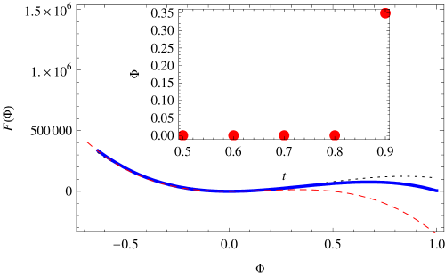
Figure 1: (Color online) The effective PNJL free energy as a function of the Polyakov-loop parameter with $T<T_{CD}$ (Black-Dotted), $T=T_{CD}$ (Blue-Thick), and $T>T_{CD}$ (Red-Dashed). Inset: The Polyakov-loop parameter as a function of temperature scaled with $T_{0}$. The Polyakov-loop parameter vanishes in $T<T_{CD}$, causing confinement, while it becomes condensed in $T>T_{CD}$, resulting in deconfinement.

Interestingly, the result in the mean-field approach of the PNJL model implies that the condensation of holons is not allowed, since $D[\Phi,\mu]=1-2\Phi\exp{[-\beta(q^{2}/2m_{h}-\mu)]}+\exp{[-2\beta(q^{2}/2m_{h}-\mu)]}$ of the holon sector in Eq.(23) cannot reach the zero value because of $0\leq\Phi<1$ except for $\Phi=1$. In other words, Higgs phenomena are not compatible with the confinement in this description, being not inconsistent with the previous field-theoretic result Higgs_Confinement . It should be also noted that the mean-field approximation does not take into account feedback effects from matters to gauge fluctuations. In fact, The fluctuations of the Fermi surface are not introduced, so that Landau-damped dynamics for gauge fluctuations is still missing. Thus, it is desirable to introduce quantum corrections beyond the mean-field approximation in the PNJL, which is the main topic of the work.

Since the Higgs phase is not allowed in the presence of the Polyakov-loop order parameter, an immediate issue boils down to how to describe the Fermi liquid phase. We will now examine the electron self-energy in the confinement phase, certainly recovering the Fermi liquid self-energy proportional to $\omega^{2}$ with frequency $\omega$ below a certain temperature associated with the holon chemical potential or the holon mass gap.

III Crossover from non-Fermi liquid to Fermi liquid

The central question of the present study is about the fate of the spinons and holons when the Polyakov-loop parameter vanishes. The spinon-holon coupling term in Eq. (16) can be expressed as follows

$$\mathcal{S}_{\mathrm{el}}\;=\;\int_{0}^{\beta}d\tau\int d^{2}r\left(\psi_{\sigma n}^{\dagger}h_{n}c_{\sigma}+c_{\sigma}^{\dagger}h^{\dagger}_{p}\psi_{\sigma p}-\frac{1}{g_{I}}c_{\sigma}^{\dagger}c_{\sigma}\right),$$ (27)

where $\sigma$ and $n(p)$ represent spin and SU(2) indices, respectively. Since the Grassmann variable $c_{\sigma}$ carries exactly the same quantum numbers as the electron, one may identify it as the Hubbard-Stratonovich field $c_{\sigma}$. The effective coupling constant $g_{I}$ plays a role of the chemical potential for the electrons. Note that the Fermi surface of the electrons differs from that of the spinons in principle.

One can introduce quantum corrections self-consistently in the Luttinger-Ward functional approach LW , in which only self-energy diagrams are taken into account, vertex corrections Kim_LW being ignored,

$$F_{LW}[\phi,\mu;\delta,T] = -\frac{1}{\beta}\sum_{i\omega}\sum_{k}\Bigl{\{}\ln\Bigl{(}-G^{\psi-1}_{\sigma\sigma,pp^{\prime}}(k,i\omega)\Bigr{)}+\Sigma^{\psi}_{\sigma\sigma,pp^{\prime}}(k,i\omega)G^{\psi}_{\sigma\sigma,p^{\prime}p}(k,i\omega)\Bigr{\}}$$ (31)

$$-\;\frac{1}{\beta}\sum_{i\omega}\sum_{k}\Bigl{\{}\ln\Bigl{(}-G^{c-1}_{\sigma\sigma}(k,i\omega)\Bigr{)}+\Sigma^{c}_{\sigma\sigma}(k,i\omega)G^{c}_{\sigma\sigma}(k,i\omega)\Bigr{\}}$$

$$+\;\frac{1}{\beta}\sum_{i\Omega}\sum_{q}\Bigl{\{}\ln\Bigl{(}-G^{h-1}_{pp^{\prime}}(q,i\Omega)\Bigr{)}+\Sigma^{h}_{pp^{\prime}}(q,i\Omega)G^{h}_{p^{\prime}p}(q,i\Omega)\Bigr{\}}$$

$$-\;\frac{1}{\beta}\sum_{i\omega}\sum_{k}\frac{1}{\beta}\sum_{i\Omega}\sum_{q}G^{c}_{\sigma\sigma}(k+q,i\omega+i\Omega)G^{h}_{p^{\prime}p}(q,i\Omega)G^{\psi}_{\sigma\sigma,pp^{\prime}}(k,i\omega)+\mu\delta+\mu_{s}\,.$$

Here, $G^{c}_{\sigma\sigma}(k,i\omega)$, $G^{\psi}_{\sigma\sigma,pp^{\prime}}(k,i\omega)$, and $G^{h}_{pp^{\prime}}(q,i\Omega)$ represent the single-particle Green functions for confined electrons, spinons, and holons, respectively, written as

$$-G^{c-1}_{\sigma\sigma}(k,i\omega) = \Sigma^{c}_{\sigma\sigma}(k,i\omega)-g_{I}^{-1},$$ (32)

$$-G^{\psi-1}_{\sigma\sigma,pp^{\prime}}(k,i\omega) = [-i(\omega+p\phi)-p\mu_{s}]\delta_{pp^{\prime}}+\frac{k^{2}}{2m_{\psi}}\delta_{pp^{\prime}}+\Sigma^{\psi}_{\sigma\sigma,pp^{\prime}}(k,i\omega),$$ (33)

$$-G^{h-1}_{pp^{\prime}}(q,i\Omega) = [-i(\Omega+p\phi)-\mu]\delta_{pp^{\prime}}+\frac{q^{2}}{2m_{h}}\delta_{pp^{\prime}}+\Sigma^{h}_{pp^{\prime}}(q,i\Omega),$$ (34)

where $\Sigma^{c}_{\sigma\sigma}(k,i\omega)$, $\Sigma^{\psi}_{\sigma\sigma,pp^{\prime}}(k,i\omega)$, and $\Sigma^{h}_{pp^{\prime}}(q,i\Omega)$ designate the self-energy corrections for confined electrons, spinons, and holons, respectively. This approximation is referred to as the Eliashberg theory that was previously believed to be valid in the large-$N$ limit FMQCP , where $N$ represents the spin degeneracy. However, the validity of the large-$N$ limit has been questioned SungSik_Genus ; Metlitski_Sachdev1 ; Metlitski_Sachdev2 recently, which will be discussed in the final section.

Having minimized the free energy with respect to each self-energy

$$\frac{\partial F_{LW}(x,T)}{\partial\Sigma^{c}_{\sigma\sigma}(k,i\omega)}=0,~{}~{}~{}~{}~{}\frac{\partial F_{LW}(x,T)}{\partial\Sigma^{\psi}_{\sigma\sigma,pp^{\prime}}(k,i\omega)}=0,~{}~{}~{}~{}~{}\frac{\partial F_{LW}(x,T)}{\partial\Sigma^{h}_{pp^{\prime}}(q,i\Omega)}=0\,,$$ (35)

we find the self-consistent equations for the self-energies as follows

$$\Sigma^{c}_{\sigma\sigma}(k,i\omega) = -\frac{1}{\beta}\sum_{i\Omega}\sum_{q}G^{h}_{p^{\prime}p}(q,i\Omega)G^{\psi}_{\sigma\sigma,pp^{\prime}}(k-q,i\omega-i\Omega),$$ (36)

$$\Sigma^{\psi}_{\sigma\sigma,pp^{\prime}}(k,i\omega) = -\frac{1}{\beta}\sum_{i\Omega}\sum_{q}G^{c}_{\sigma\sigma}(k+q,i\omega+i\Omega)G^{h}_{p^{\prime}p}(q,i\Omega),$$ (37)

$$\Sigma^{h}_{pp^{\prime}}(q,i\Omega) = \frac{1}{\beta}\sum_{i\omega}\sum_{k}G^{c}_{\sigma\sigma}(k+q,i\omega+i\Omega)G^{\psi}_{\sigma\sigma,pp^{\prime}}(k,i\omega)\,.$$ (38)

These equations were intensively discussed in the context of heavy fermions Pepin_Paul without the confinement, i.e., without the Polyakov-loop parameter. Thus, this framework may be regarded as an extension of the mean-field analysis, both the confinement effects and the quantum fluctuations being incorporated self-consistently.

In the confinement phase the spectral function of the spinon should not be reduced to the delta function owing to the presence of the background potential $\phi$ even if the self-energy correction is ignored. Actually, the Polyakov-loop parameter plays a role of the imaginary part of the self-energy, which makes the spinon resonance disappear as shown in the first panel of Fig. 2. The holon spectrum also features a broad structure, presented in the second panel of Fig. 2. It indicates that both the spinon and the holon are not well-defined excitations in the confinement phase. On the other hand, the electron as a spinon-holon composite exhibits a rather sharp peak in the last graph of Fig. 2, since the imaginary part of their self-energy vanishes at the Fermi surface in spite of no pole structure in the electron Green function.

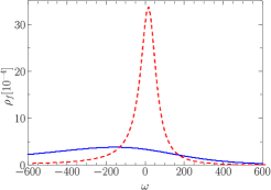
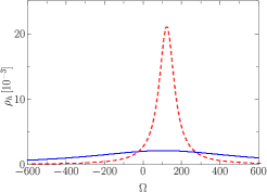
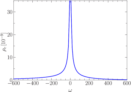
Figure 2: (Color online) Spinon, holon, and electron spectra: The Polyakov-loop parameter gives rise to huge imaginary parts for self-energies of both spinons and holons in the confinement region, making the spinon and holon spectra broader (blue thick curve). On the other hand, electron excitations become rather sharply defined due to confinement, but not fully coherent at high temperatures, which originates from strong inelastic scattering with such incoherent spinon and holon excitations.

The holon self-energy is found to be of the standard form in two dimensions:

$$\Sigma_{p}^{b}(q,i\Omega)-\Sigma_{p}^{b}(q,0) = -\frac{\rho_{c}}{i(\alpha-1)}\Bigl{\{}\tan^{-1}\Bigl{(}\frac{i\Omega+ip\phi-v_{F}^{c}q^{*}+v_{F}^{c}q}{-i\Omega-ip\phi+v_{F}^{c}q^{*}+v_{F}^{c}q}\Bigr{)}$$ (40)

$$\hskip 42.67912pt-\tan^{-1}\Bigl{(}\frac{i\Omega+ip\phi-\alpha v_{F}^{c}q^{*}+\alpha v_{F}^{c}q}{-i\Omega-ip\phi+\alpha v_{F}^{c}q^{*}+\alpha v_{F}^{c}q}\Bigr{)}\Bigr{\}}$$

except for $i\Omega\rightarrow i\Omega+ip\phi$. The $\rho_{c}$ denotes the density of states for the confined electron, and $v_{F}^{c}$ stands for the corresponding Fermi velocity. The $\alpha$ represents the ratio of the electron band mass to the spinon one, given as almost unity. The $q^{*}$ designates the Fermi-momentum mismatch between the confined electron and the spinon. A detailed derivation is shown in Appendix B.

Inserting Eq. (40) into the electron self-energy equation, we can find its explicit form. See Appendix C for its derivation. An important energy scale is given by the holon chemical potential $\mu$. In $T>|\mu|$, holon dynamics is described by the dynamical exponent $z=3$, resulting from the Landau damping of the electron and spinon Kim_LW ; Pepin_Paul . The imaginary part of the self-energy turns out to be proportional to $T^{2/3}$, since the confined electrons are scattered with such $z=3$ dissipative modes Kim_LW ; Pepin_Paul . On the other hand, the holon excitations have gaps in $T<|\mu|$, so that scattering with confined electrons are suppressed, which recovers the Fermi liquid. Thus, the Fermi liquid appears as the coherence effect in the confinement phase rather than the Higgs phase in the deconfinement state. This mechanism resolves the artificial transition at finite temperatures.

Figure 3: (Color online) The results of the electrical resistivity are drawn as a function of temperature. The circle, triangle, and lozenge denote the experimental data Data corresponding to different values of the doping. The non-Fermi liquid electrical resistivity Data_fitting evolves into the typical Fermi-liquid behavior below the crossover temperature, given by the holon gap.

The coherence crossover can be manifestly observed in the electrical transport. It should be realized that the Ioffe-Larkin composition rule for the transport IoffeLarkin does not apply to the confinement phase. Instead, the electrical currents would be carried by confined electrons dominantly. This is in sharp contrast with the existing gauge-theoretic description for the SM phase, where the anomalous electrical transport originates from holon dynamics interacting with gauge fluctuations SM_U1GT . In addition to this important aspect, the relaxation time associated with the imaginary part of the self-energy differs from the transport time, and the back scattering contribution is factored out by the vertex corrections. Actually, the role of the vertex corrections has been investigated carefully in the context of the heavy fermion quantum criticality of the Kondo breakdown Pepin_Paul ; Kim_TR ; Kim_QBE_KB . Employing the quantum Boltzmann equation approach, Refs. Pepin_Paul ; Kim_TR ; Kim_QBE_KB have shown that the backscattering contribution selected from the vertex corrections is given by $1-\alpha\cos\theta$ in the scattering mechanism from spinon-holon binding fluctuations, where $\theta$ is an angle measured from the direction of the electric current. An important point is that this scattering mechanism introduces the factor $\alpha$, which is negligibly small in the Kondo breakdown scenario, because the band mass of the spinons is large due to the $f$-orbital character. On the other hand, we should have $\alpha\approx 1$ in the SM phase because the band mass of the spinons is almost identical with that of the emergent electrons. In this case the vertex corrections should be introduced. Their temperature dependence is well known to be proportional to $T^{2/3}$ for two dimensional $z=3$ fluctuations Kim_TR .

Introducing both the self-energy and vertex corrections, we reach the final expression of the electrical resistivity

$$\rho_{el}(T)\;=\;\rho_{0}+\mathcal{C}\Bigl{(}N_{s}\rho_{c}\frac{v_{F}^{c2}}{3}\Bigr{)}^{-1}T^{2/3}Im[\Sigma_{c}(T)]\,,$$ (41)

where $\rho_{0}$, $\mathcal{C}$, and $N_{s}$ denote, respectively, the residual resistivity due to disorder, the strength for the vertex corrections, and the spin degeneracy, among which $\rho_{0}$ and $\mathcal{C}$ are free parameters. Note that the $T^{2/3}$ factor results from the vertex corrections. As shown in Fig. 3, the results are in remarkable agreement with the experimental data, which supports our confinement scenario. In addition, the $T^{2}$ behavior is clearly observed at low temperatures, confirming our statement that the crossover from the SM phase to the Fermi liquid state is described by the coherence effect with the confinement.

IV Conclusion : Loose end

In the present study we proposed a novel mechanism for the marginal Fermi-liquid phenomenology near optimal doping in high $T_{c}$ cuprates. First, we tried to resolve the artificial finite-temperature second-order transition from a spinon-holon deconfined non-Fermi liquid state (or a finite-temperature spin-liquid state) to a spinon-holon Higgs-confined Fermi-liquid phase. Indeed, we made the continuous transition smoothen into the crossover, but from a spinon-holon confined incoherent Fermi-liquid state to a spinon-holon confined coherent Fermi-liquid phase. The confinement of spinons and holons at finite temperatures was phenomenologically described by the Polyakov-loop parameter, where confined spinon-holon composite particles are identified with incoherent electrons in the temperature-regime above the ”holon” chemical potential. Although holons are not elementary excitations due to confinement, given by the huge imaginary part from the Polyakov-loop parameter, their chemical potential defines the coherence energy scale.

The second point, which is more important in our opinion, is that we proposed one possible mechanism for the non-Fermi liquid resistivity near the optimal doping, introducing the Polyakov-loop parameter. This object gives rise to not only confinement but also an interesting self-energy correction to such confined spinons, where the imaginary part of the spinon self-energy is proportional to temperature, regarded as the signature of confinement. This anomalous dynamics affects dynamics of incoherent electrons, responsible for the non-Fermi liquid resistivity above the Fermi-liquid coherence temperature near the optimal doping. We believe that this is a novel mechanism for the non-Fermi liquid transport around the optimal doping in high $T_{c}$ cuprates. In order to realize such non-Fermi liquid physics, we usually resort to some type of critical fluctuations, which can give rise to the T-linear self-energy correction. Recall the marginal Fermi-liquid Ansatz. In this study we do not assume any kinds of symmetry breaking for the scattering mechanism. The Polyakov-loop parameter serves a novel scattering mechanism for the marginal Fermi-liquid physics near the optimal doping.

In fact, we cannot justify the fundamental reason why the Polyakov-loop parameter should be utilized near optimal doping. Our formulation is based on a spin liquid state, expected to apply to an underdoped paramagnetic insulating-like state (at least applicable to finite temperatures, usually referred to as the proximity effect of the spin liquid physics), where spinons and holons appear as elementary excitations. Although we cannot explain how such deconfined particles evolve into confined electrons as a function of hole concentration, we believe that these deconfined excitations should be confined around the optimal doping region above the pseudogap phase, where the anomalous $T$-linear-like resistivity is shown. An important question is how to construct incoherent electrons from spinons and holons at finite temperatures. One can introduce a spinon-holon bound state based on the ladder-type t-matrix approximation without the Polyakov-loop parameter. However, it is not clear whether this construction allows the non-Fermi liquid resistivity or not. We would like to emphasize again that the Polyakov-loop parameter can solve two problems at the same time, confinement (conceptually valid) and non-Fermi liquid (marginal Fermi liquid) physics near the optimal doping.

If one insists that deconfinement should be stabilized due to the Fermi surface SungSik_Deconfinement and the confined Fermi liquid state results from the Anderson-Higgs mechanism, we would like to point out that the existence argument can be justified in the large-$N$ limit, where $N$ is the number of degeneracy in fermion flavors. If we consider a realistic situation at finite $N$, several types of missing correlations may play an important role for fermion dynamics, where enhanced correlations will reduce conductivity, which means that such fermions can have difficulty in screening gauge interactions. It is natural to expect that fermions in an almost insulating state will not screen gauge forces appropriately, even if they form their Fermi surface Kim_FS_Deconfinement . Although we cannot give any definite statement on confinement in the presence of the Fermi surface, we believe that there is no consensus, in particular, when finite $N$ should be considered Finite_N_Confinement . What we can argue here is that our confinement formulation based on the Polyakov-loop parameter turns the artificial second-order transition into the crossover, conceptually more advantageous than the holon condensation.

One may suspect whether our Fermi liquid state is the genuine Fermi liquid phase or not because it is not obvious that the Fermi surface of such coherent electrons satisfies the Luttinger theorem Luttinger_Theorem . The main quantity is the chemical potential of electrons, emerging from confinement of spinons and holons. Although this quantity should be and can be determined self-consistently in our formulation, we did not perform such a serious analysis. That analysis will involve many delicate issues, for example, a more accurate expression of the self-energy correction of electrons in order to determine the chemical potential accurately. In our study we just introduce the electron chemical potential phenomenologically, which can be determined to satisfy the Luttinger theorem. This is the best at present in our formulation, which is another reason why we call our theory a phenomenological description.

We would like to point out that the issue on the formation of incoherent electrons from deconfined spinons and holons is not seriously discussed in our study. Incoherent electrons are assumed to exist at finite temperatures around the optimal doping region, resorting to the Polyakov-loop parameter. Of course, we pointed out that spinons and holons can be deconfined at high temperatures, showing that the Polyakob-loop parameter is non-vanishing in the saddle-point approximation. In our mean-field analysis the change from the spinon-holon deconfined state to the confined incoherent Fermi-liquid state (by Polyakov loop) is naturally interpreted as the crossover at finite temperatures (much higher than the non-Fermi liquid to Fermi liquid crossover temperature) because there is no symmetry breaking, as discussed before. Unfortunately, it doesn’t seem to be clear whether it is crossover or not beyond the mean-field analysis, which means to introduce quantum fluctuations for the Polyakov-loop parameter Deconfinement_KT . It is also an open question in our description how the Polyakov-loop parameter evolves by hole doping. We believe that this requires some modifications of our present formulation.

One may criticize cautiously the Eliashberg approximation for neglecting the vertex corrections for self-energies. It has been recently clarified that two dimensional Fermi surface is still strongly interacting even in the large-$N$ limit SungSik_Genus ; Metlitski_Sachdev1 ; Metlitski_Sachdev2 ; McGreevy ; Kim_Ladder ; Kim_AL , which implies that vertex corrections should be incorporated. An important question is raised as to whether these vertex corrections give rise to novel critical exponents beyond the Eliashberg theory. Several perturbative analysis demonstrated that although ladder-type vertex corrections do not change the critical exponents of the Eliashberg theory, Aslamasov-Larkin corrections bring about modifications for such critical exponents Metlitski_Sachdev1 ; Metlitski_Sachdev2 . If this is a general feature beyond this level of approximation, various quantum critical phenomena HFQCP should be reconsidered because the novel anomalous exponents in the fermion self-energy corrections are expected to affect various novel critical exponents for thermodynamics, transport, etc. However, considering our recent experiences in comparison with various experiments in heavy fermion quantum criticality, we want to emphasize that the critical exponents based on the Eliashberg theory explain thermodynamics Kim_Adel_Pepin , both electrical and thermal transport coefficients Kim_TR , uniform spin susceptibility Kim_Jia , and Seebeck effect Kim_Pepin_Seebeck noticeably well.

Recently, one of the authors investigated the role of the vertex corrections non-perturbatively, summing them to infinite order Kim_Ladder ; Kim_AL . It turns out that particular vertex corrections given by ladder diagrams do not change Eliashberg critical exponents at all Kim_Ladder , being consistent with the perturbative analysis. This was performed in a fully self-consistent way, the Ward identity being utilized. In contrast with the previous perturbative analysis, the Aslamasov-Larkin corrections were shown not to modify the Eliashberg dynamics Kim_AL . In analogy with superconductivity, where the superconducting instability described by the Aslamasov-Larkin vertex corrections is reformulated by the anomalous self-energy in the Eliashberg framework of the Nambu spinor representation BCS , we claimed that the off-diagonal self-energy associated with the 2$k_{F}$ particle-hole channel incorporates the same (Aslamasov-Larkin) class of quantum corrections in the Nambu spinor representation. We evaluated an anomalous pairing self-energy in the Nambu-Eliashberg approximation, which vanishes at zero energy but displays the same power-law dependence for the frequency as the normal Eliashberg self-energy. As a result, even the pairing self-energy corrections do not modify the Eliashberg dynamics without the Nambu spinor representation. We leave this profound and important issue for future investigations.

It will be of great interest to apply the PNJL scheme to the spin-liquid theory Spin_Liquid and Kondo breakdown scenario Pepin_Paul for heavy fermions. In particular, the artificial finite-temperature transition would be resolved for the heavy fermion transition in the same way as the present case, which may allow a new scenario of quantum criticality.

Appendix A An effective Polyakov-loop action in the one loop level from the Yang-Mills theory

Taking the reparameterization

$$a_{\mu}^{+}\;=\;\frac{a_{\mu}^{1}+a_{\mu}^{2}}{\sqrt{2}},~{}~{}~{}~{}~{}a_{\mu}^{-}=\frac{a_{\mu}^{+}-a_{\mu}^{2}}{\sqrt{2}i}\,,$$ (42)

one can rewrite the Yang-Mills action as follows

$$\mathcal{L}_{YM} = \frac{1}{4g^{2}}\Bigl{(}[\partial_{\mu}a_{\nu}^{+}-\partial_{\nu}a_{\mu}^{+}-ig(a_{\mu}^{3}a_{\nu}^{+}-a_{\nu}^{3}a_{\mu}^{+})]^{2}+[\partial_{\mu}a_{\nu}^{-}-\partial_{\nu}a_{\mu}^{-}+ig(a_{\mu}^{3}a_{\nu}^{-}-a_{\nu}^{3}a_{\mu}^{-})]^{2}$$ (44)

$$+\;[\partial_{\mu}a_{\nu}^{3}-\partial_{\nu}a_{\mu}^{3}-ig(a_{\mu}^{+}a_{\nu}^{-}-a_{\nu}^{+}a_{\mu}^{-})]^{2}\Bigr{)}$$

$$= \frac{1}{4g^{2}}\Bigl{(}[(\partial_{\tau}-iga_{\tau}^{3})a_{i}^{+}-(\partial_{i}-iga_{i}^{3})a_{\tau}^{+}]^{2}+(i\longleftrightarrow\tau)+[(\partial_{i}-iga_{i}^{3})a_{j}^{+}-(\partial_{j}-iga_{j}^{3})a_{i}^{+}]^{2}\Bigr{)}$$ (47)

$$+\;\frac{1}{4g^{2}}\Bigl{(}[(\partial_{\tau}+iga_{\tau}^{3})a_{i}^{-}-(\partial_{i}+iga_{i}^{3})a_{\tau}^{-}]^{2}+(i\longleftrightarrow\tau)+[(\partial_{i}+iga_{i}^{3})a_{j}^{-}-(\partial_{j}+iga_{j}^{3})a_{i}^{-}]^{2}\Bigr{)}$$

$$+\;\frac{1}{4g^{2}}\Bigl{(}[\partial_{\tau}a_{i}^{3}-\partial_{i}a_{\tau}^{3}-ig(a_{\tau}^{+}a_{i}^{-}-a_{i}^{+}a_{\tau}^{-})]^{2}+(i\longleftrightarrow\tau)+[\partial_{i}a_{j}^{3}-\partial_{j}a_{i}^{3}-ig(a_{i}^{+}a_{j}^{-}-a_{j}^{+}a_{i}^{-})]^{2}\Bigr{)}\,,$$

where $a_{\mu}^{3}$ is introduced as the covariant derivative for the $a_{\mu}^{\pm}$ field.

Taking the Ansatz

$$a_{\tau}^{3}=\phi,\;\;\;\;a_{i}^{3}=0$$ (48)

for the lowest-order approximation, we reach the following expression for the Yang-Mills action

$${\cal L}_{YM} \approx \frac{1}{2g^{2}}\Bigl{(}[(\partial_{\tau}-ig\phi)a_{i}^{+}-\partial_{i}a_{\tau}^{+}]^{2}+[\partial_{i}a_{j}^{+}-\partial_{j}a_{i}^{+}]^{2}\Bigr{)}+\frac{1}{4g^{2}}\Bigl{(}[(\partial_{\tau}+ig\phi)a_{i}^{-}-\partial_{i}a_{\tau}^{-}]^{2}+[\partial_{i}a_{j}^{-}-\partial_{j}a_{i}^{-}]^{2}\Bigr{)}$$ (50)

$$+\;\frac{1}{2}[a_{\tau}^{+}a_{i}^{-}-a_{i}^{+}a_{\tau}^{-}]^{2}+\frac{1}{4}[a_{i}^{+}a_{j}^{-}-a_{j}^{+}a_{i}^{-}]^{2}\,.$$

Integrating over $a_{\mu}^{\pm}$ without their interactions given by the last two terms, we obtain an effective action for the Polyakov-loop parameter in the one loop level, corresponding to Eq. (21).

Appendix B Holon self-energy with the Polyakov-loop parameter

Linearizing the band dispersion near each Fermi surface, we obtain the electron and spinon Green functions

$$G_{c}(k,i\omega) \approx \frac{1}{i\omega-v_{F}^{c}k-\Sigma_{c}(i\omega)},$$ (51)

$$G_{\psi}(k+q,i\omega+i\Omega) = \frac{1}{(i\omega+i\Omega+ip\phi)-v_{F}^{\psi}k-v_{F}^{\psi}q_{\parallel}-v_{F}^{\psi}q^{*}-\Sigma^{\psi}_{p}(i\omega+i\Omega)}\,,$$ (52)

respectively, where each self-energy correction is assumed to depend only on the frequency, which is well adopted in the Eliashberg framework FMQCP because most singular corrections result from the frequency dependence. In the electron Green function we set $\Sigma_{c}(k,i\omega)\approx\frac{k^{2}}{2m_{c}}+\Sigma_{c}(i\omega)$, and expand the dispersion near the chemical potential $g^{-1}_{I}$. The Fermi velocity $v_{F}^{\psi}$ of the spinons is related with that of the electrons as $v_{F}^{\psi}=\alpha v_{F}^{c}$, where $\alpha\approx 1$ because the band mass of the electrons is almost identical with that of the spinons. $q^{*}=k_{F}^{c}-k_{F}^{\psi}$ is the Fermi surface mismatch.

Since fermion self-energies are assumed to depend on frequency only, the boson self-energy is basically the same as that in the random-phase approximation FMQCP . Inserting the above fermion Green functions into the self-consistent equation for the boson self-energy, we obtain

$$\Sigma_{p}^{b}(q,i\Omega)-\Sigma_{p}^{b}(q,0)$$ (53)

$$\approx -\frac{\rho_{c}}{2\pi^{2}}\int_{-\infty}^{\infty}{d\omega}\int_{0}^{2\pi}{d\theta}\int_{-\infty}^{\infty}d\epsilon\frac{1}{i\omega-\epsilon}\frac{1}{(i\omega+i\Omega+ip\phi)-\alpha\epsilon-\alpha v_{F}^{c}q^{*}-\alpha v_{F}^{c}q\cos\theta}$$ (54)

$$= i\frac{\rho_{c}}{2\pi}\int_{-\infty}^{\infty}{d\omega}\int_{0}^{2\pi}{d\theta}\frac{\Theta(\omega+\Omega+p\phi)-\Theta(\omega)}{i\Omega+(1-\alpha)i\omega+ip\phi-\alpha v_{F}^{c}q^{*}-\alpha v_{F}^{c}q\cos\theta}$$ (55)

$$= \frac{\rho_{c}}{2}\int_{-\Omega-p\phi}^{0}{d\omega}\Bigl{\{}[i\Omega+(1-\alpha)i\omega+ip\phi-\alpha v_{F}^{c}q^{*}+\alpha v_{F}^{c}q][-i\Omega-(1-\alpha)i\omega-ip\phi+\alpha v_{F}^{c}q^{*}+\alpha v_{F}^{c}q]\Bigr{\}}^{-\frac{1}{2}}$$ (56)

$$= -\frac{\rho_{c}}{i(\alpha-1)}\Bigl{\{}\tan^{-1}\Bigl{(}\frac{i\Omega+ip\phi-v_{F}^{c}q^{*}+v_{F}^{c}q}{-i\Omega-ip\phi+v_{F}^{c}q^{*}+v_{F}^{c}q}\Bigr{)}-\tan^{-1}\Bigl{(}\frac{i\Omega+ip\phi-\alpha v_{F}^{c}q^{*}+\alpha v_{F}^{c}q}{-i\Omega-ip\phi+\alpha v_{F}^{c}q^{*}+\alpha v_{F}^{c}q}\Bigr{)}\Bigr{\}}\,,$$ (57)

where $\rho_{c}$ is the density of states for electrons. The $\Sigma_{p}^{b}(q,0)$ is proportional to $q^{2}$.

Appendix C Electron self-energy with the Polyakov-loop parameter

Since the boson self-energy is nothing but the typical expression in the two dimensional Fermi liquid except for the Polyakov-loop parameter, the boson self-energy is given by the Landau-damping, that is, not by $\Omega$ alone but by $\Omega+p\phi$ in the low-energy limit. Inserting this approximate boson self-energy with the damping coefficient $\gamma_{b}$ into the electron self-energy equation, we obtain

$$\Sigma^{c}(k_{F}^{c},i\omega)$$ (58)

$$= -\frac{1}{\beta}\sum_{i\Omega}\int_{-\infty}^{\infty}\frac{dq_{\parallel}}{2\pi}\int_{-\infty}^{\infty}\frac{dq_{\perp}}{2\pi}\frac{1}{[-i(\Omega+p\phi)-\mu]+\frac{q_{\perp}^{2}}{2m_{h}}+\gamma_{b}\frac{|\Omega+p\phi|}{q_{\perp}}}$$ (60)

$$\hskip 108.12054pt\times\frac{1}{-i(\omega-\Omega+p\phi)+v_{F}^{\psi}q_{\parallel}+\Sigma^{\psi}_{p}(k_{F}^{c}-q,i\omega-i\Omega)}$$

$$\approx -\frac{1}{\beta}\sum_{i\Omega}\int_{-\infty}^{\infty}\frac{dq_{\parallel}}{2\pi}\frac{1}{-i(\omega-\Omega+p\phi)+v_{F}^{\psi}q_{\parallel}}\frac{1}{[-i(\Omega+p\phi)-\mu]+\frac{q_{\perp}^{2}}{2m_{h}}+\gamma_{b}\frac{|\Omega+p\phi|}{q_{\perp}}}\,.$$ (61)

The spectral representation being employed, the imaginary part of the electron self-energy is given by

$$Im[\Sigma^{c}(k_{F}^{c},\omega+i\delta)] = -\frac{1}{\pi}\int_{-\infty}^{\infty}\frac{dq_{\parallel}}{2\pi}\int_{-\infty}^{\infty}\frac{dq_{\perp}}{2\pi}\int_{-\infty}^{\infty}d\nu\int_{-\infty}^{\infty}d\nu^{\prime}\delta(\omega-\nu+\nu^{\prime})[n(\nu)+f(\nu^{\prime})]$$ (65)

$$\hskip 85.35826pt\times\frac{\phi+\gamma_{b}\frac{\nu}{q_{\perp}}}{\Bigl{(}\nu+\mu-\frac{q_{\perp}^{2}}{2m_{h}}-\gamma_{b}\frac{\phi}{q_{\perp}}\Bigr{)}^{2}+\Bigl{(}\phi+\gamma_{b}\frac{\nu}{q_{\perp}}\Bigr{)}^{2}}\frac{\phi}{(\nu-v_{F}^{\psi}q_{\parallel})^{2}+\phi^{2}}$$

$$-\,\frac{1}{\pi}\int_{-\infty}^{\infty}\frac{dq_{\parallel}}{2\pi}\int_{-\infty}^{\infty}\frac{dq_{\perp}}{2\pi}\int_{-\infty}^{\infty}d\nu\int_{-\infty}^{\infty}d\nu^{\prime}\delta(\omega-\nu+\nu^{\prime})[n(\nu)+f(\nu^{\prime})]$$

$$\hskip 85.35826pt\times\frac{-\phi+\gamma_{b}\frac{\nu}{q_{\perp}}}{\Bigl{(}\nu+\mu-\frac{q_{\perp}^{2}}{2m_{h}}+\gamma_{b}\frac{\phi}{q_{\perp}}\Bigr{)}^{2}+\Bigl{(}-\phi+\gamma_{b}\frac{\nu}{q_{\perp}}\Bigr{)}^{2}}\frac{-\phi}{(\nu-v_{F}^{\psi}q_{\parallel})^{2}+\phi^{2}}\,,$$

where the presence of the Polyakov-loop parameter is the key feature.

It is straightforward to integrate over $q_{\parallel}$, which yields

$$Im[\Sigma^{c}(k_{F}^{c},\omega+i\delta)]$$ (66)

$$= -\frac{1}{2\pi v_{F}^{\psi}}\int_{-\infty}^{\infty}\frac{dq_{\perp}}{2\pi}\int_{-\infty}^{\infty}d\nu\int_{-\infty}^{\infty}d\nu^{\prime}\delta(\omega-\nu+\nu^{\prime})[n(\nu)+f(\nu^{\prime})]\frac{\phi+\gamma_{b}\frac{\nu}{q_{\perp}}}{\Bigl{(}\nu+\mu-\frac{q_{\perp}^{2}}{2m_{h}}-\gamma_{b}\frac{\phi}{q_{\perp}}\Bigr{)}^{2}+\Bigl{(}\phi+\gamma_{b}\frac{\nu}{q_{\perp}}\Bigr{)}^{2}}$$ (67)

$$+ \frac{1}{2\pi v_{F}^{\psi}}\int_{-\infty}^{\infty}\frac{dq_{\perp}}{2\pi}\int_{-\infty}^{\infty}d\nu\int_{-\infty}^{\infty}d\nu^{\prime}\delta(\omega-\nu+\nu^{\prime})[n(\nu)+f(\nu^{\prime})]\frac{-\phi+\gamma_{b}\frac{\nu}{q_{\perp}}}{\Bigl{(}\nu+\mu-\frac{q_{\perp}^{2}}{2m_{h}}+\gamma_{b}\frac{\phi}{q_{\perp}}\Bigr{)}^{2}+\Bigl{(}-\phi+\gamma_{b}\frac{\nu}{q_{\perp}}\Bigr{)}^{2}}\,.$$ (68)

It is essential to notice that the background potential is given by $\phi(T)\approx\frac{\pi}{2}T$ in the confinement phase because the Polyakov-loop parameter vanishes, i.e., $\cos\beta\phi\approx 0$. Then, the potential $\phi$ has the same scaling with the frequency. It is straightforward to see that the imaginary part of the electron self-energy follows the typical expression of $z=3$ quantum criticality when $T\gg|\mu|$ because the holon excitations are effectively gapless in this regime. As a result, we have $Im[\Sigma^{c}(T)]\propto T^{2/3}$. On the other hand, the holon fluctuations become gapped in $T\ll|\mu|$, and the self-energy corrections from these fluctuations can be neglected, which gives rise to the typical Fermi liquid form $Im[\Sigma^{c}(T)]\propto T^{2}$.

References

- (1) J. Orenstein and A. J. Millis, Science 21, 468 (2000).
- (2) C. M. Varma, Z. Nussinov, W. van Saarloos, Phys. Rep. 361, 267 (2002).
- (3) Vivek Aji and C. M. Varma, Phys. Rev. Lett. 99, 067003 (2007); C. M. Varma, Phys. Rev. Lett. 83, 3538 (1999).
- (4) Ar. Abanov, Andrey V. Chubukov, J. Schmalian, arXiv:cond-mat/0107421.
- (5) Sung-Sik Lee, Phys. Rev. B 80, 165102 (2009).
- (6) P. A. Lee, N. Nagaosa, and X.-G. Wen, Rev. Mod. Phys. 78, 17 (2006).
- (7) N. Nagaosa and P. A. Lee, Phys. Rev. Lett. 64, 2450 (1990); P. A. Lee and N. Nagaosa, Phys. Rev. B 46, 5621 (1992).
- (8) P. A. Lee, Science 321, 1306 (2008); L. Balents, Nature 464, 199 (2010).
- (9) H. Takagi, B. Batlogg, H. L. Kao, J. Kwo, R. J. Cava, J. J. Krajewski, and W. F. Peck, Jr, Phys. Rev. Lett. 69, 2975 (1992).
- (10) A. M. Polyakov, Gauge Fields and Strings (Harwood Academic Publishers, New York, 1987).
- (11) S. P. Klevansky, Rev. Mod. Phys. 64, 649 (1992).
- (12) T. Hatsuda and T. Kunihiro, Phys. Rep. 247, 221 (1994).
- (13) M. Buballa, Phys. Rep. 407, 205 (2005).
- (14) T. Schäfer and E. V. Shuryak, Rev. Mod. Phys. 70, 323 (1998).
- (15) D. Diakonov, Prog. Part. Nucl. Phys. 51, 173 (2003).
- (16) K. Fukushima, Phys. Lett. B 591, 277 (2004).
- (17) A. M. Polyakov, Phys. Lett. B 72, 477 (1978).
- (18) L. Susskind, Phys. Rev. D 20, 2610 (1979).
- (19) L. D. McLerran and B. Svetitsky, Phys. Rev. D 24, 450 (1981).
- (20) B. Svetitsky, Phys. Rep. 132, 1 (1986).
- (21) C. Ratti, S. Roessner, and W. Weise, Phys. Lett. B 649, 57 (2007); S. Roessner, T. Hell, C. Ratti, and W. Weise, Nucl. Phys. A 814, 118 (2008).
- (22) K. Fukushima, Phys. Rev. D 79, 074015 (2009); W.-J. Fu, Z. Zhang, and Y.-X. Liu, Phys. Rev. D 77, 014006 (2008).
- (23) T.-K. Ng, Phys. Rev. B 71, 172509 (2005).
- (24) Ian Affleck, Z. Zou, T. Hsu, and P. W. Anderson, Phys. Rev. B 38, 745 (1988); Elbio Dagotto, Eduardo Fradkin, and Adriana Moreo, Phys. Rev. B 38, 2926 (1988).
- (25) Do not confuse the SU(2) slave-boson representation of the t-J model with the U(1) slave-boson representation of the Hubbard model [G. Kotliar and A. E. Ruckenstein, Phys. Rev. Lett. 57, 1362 (1986)], where the presence of charge fluctuations in the Hubbard model introduces the so called doublon field. The boson differs from the doublon field, where excitations of bosons describe additional low energy fluctuations associated with spin degrees of freedom while excitations of doublon bosons do charge fluctuations.
- (26) The under-doped region at intermediate temperatures is characterized by with , , and , which is known as the staggered flux (SF) phase, where the spinons have the Dirac spectrum due to the staggered internal flux whereas coherent electrons are not seen as the SM phase. Because the electron spectrum exhibits its spectral gap except for Dirac points, this SF state is identified with the so-called pseudogap phase in high Tc cuprates. Superconductivity arises from the condensation of the holons and due to in the SF phase.
- (27) We would like to emphasize that the quadratic dispersion for both spinon and holon dynamics is not valid in the underdoped region, where the stable mean-field phase turns out to be the SF phase, which gives rise to relativistic dispersions to both fermions and bosons. As a result, an effective field theory should be given by a relativistic SU(2) gauge theory except for the holon sector, where its small chemical potential breaks the relativistic invariance slightly. The chemical potential does not arise in the spinon sector for the SF phase.
- (28) K. A. Chao, J. Spalek and A. M. Oles, J. Phys. C: Solid State Phys. 10, L271 (1977).
- (29) C. Mudry and E. Fradkin, Phys. Rev. B 49, 5200 (1994); C. Mudry and E. Fradkin, Phys. Rev. B 50, 11409 (1994).
- (30) N. Weiss, Phys. Rev. D 24, 475 (1981).
- (31) N. Nagaosa and P. A. Lee, Phys. Rev. B 61, 9166 (2000); E. Fradkin and S. H. Shenker, Phys. Rev. D 19, 3682 (1979).
- (32) J. M. Luttinger and J. C. Ward, Phys. Rev. 118, 1417 (1960).
- (33) A. Benlagra, K.-S. Kim, C. Pépin, J. Phys.: Condens. Matter 23, 145601 (2011).
- (34) J. Rech, Pépin, and A. V. Chubukov, Phys. Rev. B 74, 195126 (2006).
- (35) Max A. Metlitski and S. Sachdev, Phys. Rev. B 82, 075127 (2010).
- (36) Max A. Metlitski and S. Sachdev, Phys. Rev. B 82, 075128 (2010).
- (37) I. Paul, C. Pépin, and M. R. Norman, Phys. Rev. B 78, 035109 (2008); C. Pépin, Phys. Rev. B 77, 245129 (2008).
- (38) L. B. Ioffe and A. I. Larkin, Phys. Rev. B 39, 8988 (1989).
- (39) K.-S. Kim and C. Pépin, Phys. Rev. Lett. 102, 156404 (2009); K.-S. Kim and C. Pépin, J. Phys.: Condens. Matter 22, 025601 (2010).
- (40) Ki-Seok Kim, arXiv:1104.4867, to be published in Phys. Rev. B.
- (41) If one sees our fitting curve carefully, the theoretical line of the resistivity is not completely linear in temperature, but slightly concave. Although the resistivity data near the optimally doped region has been fitted by the T-linear behavior, our demonstration shows that not only the T-linear form but also a slightly concave expression can fit the data qualitatively well.
- (42) Sung-Sik Lee, Phys. Rev. B 78, 085129 (2008).
- (43) Ki-Seok Kim, Phys. Rev. B 72, 245106 (2005).
- (44) If we review recent studies Dirac_Deconfinement ; SungSik_Deconfinement on deconfinement in compact U(1) gauge theories critically, we can understand that the essential argument for the existence of the deconfinement state is based on interacting fixed points in the large- limit. Ref. Dirac_Deconfinement is on the compact U(1) gauge theory with Dirac fermions. The authors assume the well-known conformally invariant fixed point of the non-compact QED3 (two space and one time dimensional quantum electrodynamics) in the large- limit, where vertex corrections can be neglected in the 1/ expansion. However, we would like to point out that if we consider the case with finite , antiferromagnetic correlations, underestimated for the fixed point in the large- limit, will be enhanced. See Ref. Kim_AL , where this issue was discussed in section II-A. It is possible that essential properties of the interacting fixed point in the large- limit may be changed and this fixed point would become unstable toward a novel fixed point with more enhanced staggered-spin correlations. This is important because the dynamics of Dirac fermions at the large- fixed point should be modified, which means that such fermions may have difficulty in screening gauge interactions. The Fermi surface problem is more complicated. A recent study SungSik_Deconfinement has claimed that the presence of abundant soft modes around the Fermi surface will allow the deconfinement at least in the large- limit. Although we think that this is certainly plausible, we would like to argue that it is difficult to claim its existence with confidence, in particular, at finite . First of all, 2kF correlations should have been emphasized in the strange metal phase 2kF_Instability , certainly missed in this analysis. It is difficult to guarantee the deconfinement in the presence of 2kF correlations because such correlations can reduce conductivity of spinons, expected to reduce the ability of screening for gauge interactions. Actually, one of the authors revisited this problem, and claimed that the confinement-deconfinement transition was argued to take place, depending on the spinon conductivity Kim_FS_Deconfinement .
- (45) J. Feldman, H. Knorrer, and E. Trubowitz, Commun. Math. Phys. 247, 1 (2004); A. Praz, J. Feldman, H. Knorrer, and E. Trubowitz, Europhys. Lett. 72, 49 (2005).
- (46) Hagen Kleinert, Flavio S. Nogueira, and Asle Sudbo, Phys. Rev. Lett. 88, 232001 (2002); Hagen Kleinert, Flavio S. Nogueira, and Asle Sudbo, Nucl. Phys. B 666, 361 (2003).
- (47) David F. Mross, J. McGreevy, H. Liu, and T. Senthil, Phys. Rev. B 82, 045121 (2010).
- (48) Ki-Seok Kim, Phys. Rev. B 82, 075129 (2010).
- (49) Ki-Seok Kim, Phys. Rev. B 83, 035123 (2011).
- (50) P. Gegenwart, Q. Si, and F. Steglich, Nature Physics 4, 186 (2008); H. v. Lohneysen, A. Rosch, M. Vojta, and P. Wolfle, Rev. Mod. Phys. 79, 1015 (2007).
- (51) K.-S. Kim, A. Benlagra, and C. Pépin, Phys. Rev. Lett. 101, 246403 (2008).
- (52) K.-S. Kim and C. Jia, Phys. Rev. Lett. 104, 156403 (2010).
- (53) K.-S. Kim and C. Pépin, Phys. Rev. B 83, 073104 (2011); K.-S. Kim and C. Pépin, Phys. Rev. B 81, 205108 (2010).
- (54) J. R. Schrieffer, Theory of Superconductivity (Westview Press, Colorado, 1999).
- (55) M. Hermele, T. Senthil, M. P. A. Fisher, P. A. Lee, N. Nagaosa, and X.-G. Wen, Phys. Rev. B 70, 214437 (2004).
- (56) B. L. Altshuler, L. B. Ioffe, and A. J. Millis, Phys. Rev. B 50, 14048 (1994).