Full counting statistics of level renormalization in electron transport through double quantum dots

Abstract

We examine the full counting statistics of electron transport through double quantum dots coupled in series, with particular attention being paid to the unique features originating from the level renormalization. It is clearly illustrated that the energy renormalization gives rise to a dynamical charge blockade mechanism, which eventually results in a super–Poissonian noise. Coupling of the double dots to an external heat bath leads to dephasing and relaxation mechanisms, which are demonstrated to suppress the noise in a unique way.

I Introduction

The manifestation of quantum coherence in finite systems is the foundations of mesoscopic physics. Double quantum dots van der Wiel et al. (2003); Brandes (2005), due to their inherent quantum coherence, are widely accepted as promising candidates for building scalable qubits Loss and DiVincenzo (1998); Vrijen et al. (2000); Friesen et al. (2003) and quantum states detectors Jiao et al. (2007); Gilad and Gurvitz (2006) towards the realization of quantum computation Nielsen and Chuang (2000). A great deal of effort has been invested to coherently measure, characterize and manipulate the quantum states in a double dot structure via coupling to a classic field or external surrounding Ono et al. (2002); Hayashi et al. (2003); Petta et al. (2005); Koppens et al. (2006); Fujisawa et al. (2006); Gustavsson et al. (2008); Sasaki et al. (2009).

It is well–known that a quantum system loses coherence due to coupling with a noisy environment. The involving issues have been the subject of intense research for many years Leggett et al. (1987); Weiss (2008); Yan and Xu (2005). Yet there is another important consequence of the system–environment coupling which renormalizes the internal energy of a quantum system. It has been revealed that, in a spin valve structure, the energy renormalization provides as an effective exchange magnetic field which leads to spin precession König and Martinek (2003); Braun et al. (2006); Sothmann and König (2010). For a quantum dot Aharonov–Bohm interferometer, the level renormalization gives rise to additional dephasing of the quantum state Marquardt and Bruder (2003), as well as bias dependent phase shift and asymmetric interference patterns Bruder et al. (1996). Even in solid–state quantum state measurement, the level renormalization was shown to play essential roles, and influence the measurement effectiveness crucially Luo et al. (2009, 2010a). It is therefore of vital importance to take this feature into account in order to correctly understand and analyze the electron transport properties.

To have a specific example, we will investigate the energy renormalization of electron transport through a serial double quantum dot system, as schematically shown in Fig. 1. The analysis is based on the full counting statistics (FCS), which is capable of characterizing the correlations between charge transport events of all orders Levitov et al. (1996); Bagrets and Nazarov (2003). It thus serves as an essential tool superior to the average current in distinguishing various transport mechanisms involved Blanter and Büttiker (2000); Nazarov (2003). We demonstrate unambiguously that the level renormalization gives rise to a dynamical charge blockade mechanism, which eventually results in a pronounced super–Poissonian noise. Close relation between the super–Poissonian noise and the negative differential conductance (NDC) owing to the level shift are revealed. It is further illustrated that the noise can be strongly suppressed due to coupling with an external phonon bath.

The paper is structured as follows. In Sec. II we present the model Hamiltonian for the double dot transport system. Section III is devoted to the theory of FCS. The bias voltage dependence of the level renormalization and its influence on the FCS are discussed in Sec. IV, which is then followed by the summary in Sec. V.

II Model description

Figure 1: Schematic illustration for transport through serial double quantum dots.

The system under study is schematically shown in Fig. 1, where the double dots are coupled in series. The entire system is described by the Hamiltonian

$$H=H_{\rm B}+H_{\rm S}+H^{\prime}.$$ (1)

The first part $H_{\rm B}=\sum_{\alpha={\rm L},{\rm R}}\sum_{k,\sigma}\varepsilon_{\alpha k}c_{\alpha k\sigma}^{\dagger}c_{\alpha k\sigma}$ models the noninteracting electrons in the electrodes. Here $c_{\alpha k\sigma}$ ($c_{\alpha k\sigma}^{\dagger}$) denotes the annihilation (creation) operator for electrons in the left ($\alpha$= L) or right ($\alpha$= R) electrode with spin $\sigma=\uparrow$ or $\downarrow$. The electron reservoirs are assumed to be in local equilibrium, so they are characterized by the Fermi functions $f_{{\rm L}/{\rm R}}(\omega)$. Electron transport is achieved by applying a bias voltage $V$, which is dropped symmetrically at the left and right tunnel junctions. The bias then is modeled by different chemical potentials in the left and right electrodes $\mu_{{\rm L}/{\rm R}}=\pm V/2$. Throughout this work, we set $e=\hbar=1$ for electron charge and the Planck constant, unless stated otherwise.

The second part of the Hamiltonian depicts the coupled dots:

$$H_{\rm S} = \sum_{\alpha={\rm L},{\rm R}}\left[\sum_{\sigma}E_{\alpha}n_{\alpha\sigma}+U_{0}n_{\alpha\uparrow}n_{\alpha\downarrow}\right]+U^{\prime}n_{\rm L}n_{\rm R}$$ (2)

$$+\,\Omega\sum_{\sigma}(d_{{\rm L}\sigma}^{\dagger}d_{{\rm R}\sigma}+d_{{\rm R}\sigma}^{\dagger}d_{{\rm L}\sigma}).$$

Here, $n_{\alpha\sigma}=d_{\alpha\sigma}^{\dagger}d_{\alpha\sigma}$ and $n_{\alpha}=\sum_{\sigma}n_{\alpha\sigma}$ are the occupation number operators for dot $\alpha$=L or R, with $d_{\alpha\sigma}$ ($d_{\alpha\sigma}^{\dagger}$) being the annihilation (creation) operator of an electron in the dot $\alpha$ with spin $\sigma$. Each quantum dot is assumed to have only one spin-degenerate energy level $E_{{\rm L}/{\rm R}}$ within the bias window. One can parametrize the levels by their average energy $\bar{E}=(E_{\rm L}+E_{\rm R})/2$ and their difference $\epsilon=E_{\rm L}-E_{\rm R}$, such that $E_{{\rm L}/{\rm R}}=\bar{E}\pm\frac{1}{2}\epsilon$. $\Omega$ accounts for the interdot tunneling between the coupled dots. Simultaneous occupation of one electron in each dot is associated with the interdot charge energy $U^{\prime}$. Double occupation on the same dot cost the intradot charge energy $U_{0}$, which is assumed to be much larger than the bias voltage, such that charge states with three or more electrons in the double dots are prohibited.

The third part $H^{\prime}=\sum_{\alpha,\sigma}(f_{\alpha\sigma}d_{\alpha\sigma}^{\dagger}+d_{\alpha\sigma}f_{\alpha\sigma}^{\dagger})$ describes electron tunneling between the dots and electrodes, with $f_{\alpha\sigma}\equiv\sum_{k}t_{\alpha k}c_{\alpha k\sigma}$. The effects of the stochastic electron reservoirs are encapsulated in the correlation functions $C^{(+)}_{\alpha\sigma\sigma^{\prime}}(t-\tau)\equiv\langle f_{\alpha\sigma}^{\dagger}(t)f_{\alpha\sigma^{\prime}}(\tau)\rangle$ and $C^{(-)}_{\alpha\sigma\sigma^{\prime}}(t-\tau)\equiv\langle f_{\alpha\sigma}(t)f^{\dagger}_{\alpha\sigma^{\prime}}(\tau)\rangle$. Here, $\langle(\cdots)\rangle\equiv{\rm Tr}[(\cdots)\rho_{\rm B}]$ represents the thermal average, with $\rho_{\rm B}$ the local thermal equilibrium reservoir state. Due to the serial geometry, electrons in the left (right) electrode can only transfer to the left (right) dot. The tunnel coupling strength of electrode $\alpha$=L or R to the corresponding dot is characterized by the intrinsic line width $\Gamma_{\alpha}(\omega)=2\pi\sum_{k}|t_{\alpha k}|^{2}\delta(\varepsilon_{\alpha k}-\omega)$. In what follows, we consider only spin conserving tunneling processes and assume flat bands in the electrodes, which yields energy independent couplings $\Gamma_{\alpha}$.

III Full counting statistics

The dynamics of the reduced system is described by the reduced density matrix $\rho(t)$, which is obtained from the density matrix of the entire system by integrating out the reservoir degrees of freedom. Under the second–order Born–Markov approximation, it satisfies the quantum master equation Yan (1998)

$$\dot{\rho}(t)=-{\rm i}{\cal L}\rho(t)-{\cal R}\rho(t),$$ (3)

where the first part represents the internal dynamics on the double dots, with ${\cal L}(\cdots)\equiv[H_{\rm S},(\cdots)]$. The second term accounts for the tunnel coupling between double dots and the external electrodes. Its detailed structure will be specified soon. The quantum master equation (3) fully captures the dynamics of the reduced system; however, it is not adequate to describe the output characteristics.

We unravel the reduced density matrix $\rho(t)$ into components $\rho^{(n)}(t)$, in which “$n$” denotes the number of electrons that have been transferred to the right electrode. The resultant particle–number–resolved master equation reads Li et al. (2005a, b); Luo et al. (2007, 2008),

$$\dot{\rho}^{(n)} \!\!\!=\!\!\! -{\rm i}{\cal L}\rho^{(n)}\!\!-\!\!\frac{1}{2}\!\sum_{\sigma}\!\Bigg{\{}\!\sum_{\alpha={\rm L},{\rm R}}\!\left[d_{\alpha\sigma}^{\dagger}A_{\alpha\sigma}^{(-)}\!\rho^{(n)}\!+\!\rho^{(n)}\!A_{\alpha\sigma}^{(+)}d_{\alpha\sigma}^{\dagger}\right]$$ (4)

$$-\Big{[}\,d_{{\rm L}\sigma}^{\dagger}\,\rho^{(n)}A_{{\rm L}\sigma}^{(+)}+A_{{\rm L}\sigma}^{(-)}\rho^{(n)}d_{{\rm L}\sigma}^{\dagger}+\,d_{{\rm R}\sigma}^{\dagger}\,\rho^{(n+1)}A_{{\rm R}\sigma}^{(+)}$$

$$+\,A_{{\rm R}\sigma}^{(-)}\rho^{(n-1)}d_{{\rm R}\sigma}^{\dagger}\Big{]}+\,{\rm H.c.}\Bigg{\}},$$

where $A^{(\pm)}_{\sigma}=\sum_{\sigma}A^{(\pm)}_{\alpha\sigma}$, and $A^{(\pm)}_{\alpha\sigma}\equiv\sum_{\sigma^{\prime}}\{C^{(\pm)}_{\alpha\sigma\sigma^{\prime}}(\pm{\cal L})+{\rm i}D^{(\pm)}_{\alpha\sigma\sigma^{\prime}}(\pm{\cal L})\}d_{\alpha\sigma^{\prime}}$. Here, the involving spectral functions are defined as the Fourier transform of the bath correlation functions, i.e.,

$$C^{(\pm)}_{\alpha\sigma\sigma^{\prime}}(\pm{\cal L})=\int_{-\infty}^{\infty}\!{\rm d}t\,e^{\pm{\rm i}{\cal L}t}C^{(\pm)}_{\alpha\sigma\sigma^{\prime}}(t).$$ (5)

The dispersion function $D^{(\pm)}_{\alpha\sigma\sigma^{\prime}}(\pm{\cal L})$ then is determined via Yan and Xu (2005); Xu and Yan (2002)

$$D^{(\pm)}_{\alpha\sigma\sigma^{\prime}}(\pm{\cal L})=-\frac{{\cal P}}{\pi}\!\int_{-\infty}^{\infty}\!\!{\rm d}\omega\frac{C^{(\pm)}_{\alpha\sigma\sigma^{\prime}}(\pm\omega)}{{\cal L}-\omega},$$ (6)

with ${\cal P}$ denoting the principal part. The spectral functions are associated with particle transfer processes, and the dispersion functions account for the coupling–induced energy renormalization of the dot levels. The latter has been neglected in previous work Gurvitz and Prager (1996); Gurvitz (1997, 1998); Stoof and Nazarov (1996); Hazelzet et al. (2001), in which the Fermi energies of the electrodes are assumed to be far away from the electronic states of the dots. Later, it will be shown that the level renormalization can give rise to intriguing and important features in the output characteristics.

By summing up all the components $\rho^{(n)}(t)$ in Eq. (4), one recovers the unconditional quantum master equation. Consequently, the dissipative term in Eq. (3) is specified explicitly. The unique advantage of the particle–number–resolved master equation is its capability of establishing a close link between the reduced dynamics and the output characteristics. By utilizing the conditional master equation (4), FCS characteristics can be readily determined, which enable us to get access to the complete information of transport.

Let us start with the particle–number–resolved reduced density matrix, which is directly related to the the probability distribution $P(n,t_{0})$ of having $n$ electrons transferred through the system during the counting time $t_{0}$, i.e., $P(n,t_{0})={\rm Tr}\rho^{(n)}(t_{0})$, where the trace is over the reduced system states. The associated cumulant generating function ${\cal F}(\chi)$ is defined as

$$e^{-{\cal F}(\chi)}=\sum_{n}P(n,t_{0})e^{-{\rm i}n\chi},$$ (7)

where $\chi$ is the so–called counting field. All cumulants of the current can be obtained from the generating function by performing derivatives with respect to the counting field

$$\langle I^{k}\rangle=-\frac{1}{t_{0}}(-{\rm i}\partial\chi)^{k}{\cal F}(\chi)|_{\chi=0}.$$ (8)

The first four cumulants are related to the average current, the (zero-frequency) current shot noise, the skewness, and the kurtosis, respectively.

To derive the cumulant generating function, we shall make use of the $\chi$–space counterpart of the number–resolved reduced density matrix $\varrho(\chi,t)\equiv\sum_{n}\rho^{(n)}(t)e^{{\rm i}n\chi}$. Its equation of motion, by employing the conditional master equation (4), reads formally

$$\dot{\varrho}(\chi)\equiv{\cal L}_{\chi}\varrho(\chi),$$ (9)

where ${\cal L}_{\chi}$ is totally determined by the dynamical structure of Eq. (4). The formal solution can be readily obtained as $\varrho(\chi,t_{0})=e^{{\cal L}_{\chi}t_{0}}\varrho(\chi,0)$. Straightforwardly, the cumulant generating function reads ${\cal F}(\chi,t_{0})=-\ln\{{\rm Tr}\varrho(\chi,t_{0})\}$. Particularly, in the zero-frequency limit, i.e., the counting time $t_{0}$ is much longer than the time of tunneling through the system, the cumulant generating function is simplified to Bagrets and Nazarov (2003); Groth et al. (2006); Flindt et al. (2005); Kießlich et al. (2006)

$${\cal F}(\chi,t_{0})=-\lambda_{\rm min}(\chi)t_{0},$$ (10)

where $\lambda_{\rm min}(\chi)$ is the minimal eigenvalue of ${\cal L}_{\chi}$ that satisfies $\lambda_{\rm min}|_{\chi\rightarrow 0}\rightarrow 0$.

IV Level renormalization and FCS analysis

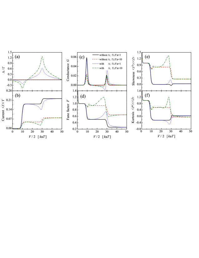
Figure 2: (a) level renormalization $\Lambda$, (b) average current $\langle I\rangle$, (c) differential conductance $G={\rm d}\langle I\rangle/{\rm d}V$, (d) Fano factor $F=\langle I^{2}\rangle/\langle I\rangle$, (e) normalized skewness, and (f) normalized kurtosis versus the bias voltage for symmetric ($\Gamma_{\rm L}=\Gamma_{\rm R}$) and asymmetric ($\Gamma_{\rm L}=10\Gamma_{\rm R}$) tunnel couplings. The bias is applied symmetrically at the left and right tunnel junctions, i.e., raise $\mu_{\rm L}=V/2$ and lower $\mu_{\rm R}=-V/2$ simultaneously. Each time when the chemical potential of the left electrode aligns with the energy needed for either single ($\bar{E}$) or double occupation ($\bar{E}+U^{\prime}$), the level renormalization reaches its local extremum. The plotting parameters are: $\epsilon$=0, $\Gamma=\Gamma_{\rm L}+\Gamma_{\rm R}=2\Omega$, $\bar{E}=10k_{\rm B}T$, $U^{\prime}=20k_{\rm B}T$, and $U_{0}=100k_{\rm B}T$.

In the strong intradot Coulomb blockade regime, double occupation on the same dot is prohibited. The involving states are restricted to: $|0\rangle$–both dots empty, $|{\rm L}\sigma\rangle$–one electron in the left dot, $|{\rm R}\sigma\rangle$–one electron in the right dot, and $|{\rm L}\sigma{\rm R}\sigma^{\prime}\rangle$–one electron in each dot, respectively. The quantum master equation (3) in this localized state representation reads

$$\dot{\rho}_{0}=-2(\Gamma_{{\rm L}}^{+}+\Gamma_{{\rm R}}^{+})\rho_{0}+\Gamma_{{\rm L}}^{-}(\rho_{{\rm L}\uparrow}+\rho_{{\rm L}\downarrow})+\Gamma_{{\rm R}}^{-}(\rho_{{\rm R}\uparrow}+\rho_{{\rm R}\downarrow}),$$ (11a)

$$\dot{\rho}_{{\rm L}\sigma}={\rm i}\Omega(\rho^{{\rm L}\sigma}_{{\rm R}\sigma}-\rho^{{\rm R}\sigma}_{{\rm L}\sigma})-(\Gamma_{\rm L}^{-}+2\tilde{\Gamma}_{{\rm R}}^{+})\rho_{{\rm L}\sigma}+\Gamma_{\rm L}^{+}\rho_{0}+\tilde{\Gamma}_{{\rm R}}^{-}(\rho_{{\rm L}\sigma{\rm R}\sigma}+\rho_{{\rm L}\sigma{\rm R}\bar{\sigma}}),$$ (11b)

$$\dot{\rho}_{{\rm R}\sigma}={\rm i}\Omega(\rho^{{\rm R}\sigma}_{{\rm L}\sigma}-\rho^{{\rm L}\sigma}_{{\rm R}\sigma})-(\Gamma_{\rm R}^{-}+2\tilde{\Gamma}_{{\rm L}}^{+})\rho_{{\rm R}\sigma}+\Gamma_{\rm R}^{+}\rho_{0}+\tilde{\Gamma}_{{\rm L}}^{-}(\rho_{{\rm L}\sigma{\rm R}\sigma}+\rho_{{\rm L}\bar{\sigma}{\rm R}\sigma}),$$ (11c)

$$\dot{\rho}_{{\rm L}\sigma{\rm R}\sigma^{\prime}}=-(\tilde{\Gamma}_{{\rm L}}^{-}+\tilde{\Gamma}_{{\rm R}}^{-})\rho_{{\rm L}\sigma{\rm R}\sigma^{\prime}}+\tilde{\Gamma}_{{\rm L}}^{+}\rho_{{\rm R}\sigma^{\prime}}+\tilde{\Gamma}_{{\rm R}}^{+}\rho_{{\rm L}\sigma},$$ (11d)

$$\dot{\rho}^{{\rm L}\sigma}_{{\rm R}\sigma}={\rm i}\,\tilde{\epsilon}\,\rho^{{\rm L}\sigma}_{{\rm R}\sigma}+{\rm i}\Omega(\rho_{{\rm L}\sigma}-\rho_{{\rm R}\sigma})-{\textstyle\frac{1}{2}}(\Gamma_{\rm L}^{-}+\Gamma_{\rm R}^{-})\rho^{{\rm L}\sigma}_{{\rm R}\sigma}-(\tilde{\Gamma}_{{\rm L}}^{+}+\tilde{\Gamma}_{\rm R}^{+})\rho^{{\rm L}\sigma}_{{\rm R}\sigma},$$ (11e)

with spin $\sigma=\{\uparrow,\downarrow\}$ and $\bar{\sigma}=-\sigma$. Here $\rho_{s}\equiv\langle s|\rho|s\rangle$ represents the diagonal element of the reduced density matrix. The off–diagonal elements $\rho^{s}_{s^{\prime}}\equiv\langle s|\rho|s^{\prime}\rangle$ describes the so–called quantum “coherencies”. The involving temperature–dependent tunneling rates are defined as $\Gamma_{\alpha}^{\pm}\equiv\Gamma_{\alpha}f_{\alpha}^{(\pm)}(\bar{E})$ and $\tilde{\Gamma}_{\alpha}^{\pm}\equiv\Gamma_{\alpha}f_{\alpha}^{(\pm)}(\bar{E}+U^{\prime})$, where $f^{(\pm)}_{\alpha}(\omega)=\{1+e^{\pm(\omega-\mu_{\alpha})/k_{{\rm B}}T}\}^{-1}$ is related to the Fermi function of the electrode $\alpha$= L or R. Here we are interested in the regime $\Delta\ll k_{\rm B}T$ ($\Delta=\sqrt{\epsilon^{2}+4\Omega^{2}}$ being the eigenenergy separation), where the external coupling strongly modifies the internal dynamics, and the off–diagonal elements of the reduced density matrix have essential roles to play Gurvitz and Prager (1996); Stoof and Nazarov (1996); Aguado and Brandes (2004). The level separation is thus smeared by the temperature, and only excitation energies $\bar{E}$ and $\bar{E}+U^{\prime}$ enters the Fermi functions.

By a close observation of the off–diagonal element of the reduced density matrix [see Eq. (11e)], it is found that the level detuning $\epsilon$ is renormalized to

$$\tilde{\epsilon}=\epsilon+\Lambda,$$ (12)

with $\Lambda=\Lambda_{\rm L}-\Lambda_{\rm R}$ the energy renormalization. The level shift $\Lambda_{\alpha}$ arising from tunnel coupling to the electrode $\alpha$ is given by

$$\Lambda_{\alpha}=\phi_{\alpha}(\bar{E})-2\phi_{\alpha}(\bar{E}+U^{\prime})+\phi_{\alpha}(\bar{E}+U_{0}),$$ (13)

with

$$\phi_{\alpha}(\omega)=\frac{\Gamma_{\alpha}}{2\pi}{\rm Re}\left[\Psi\left(\frac{1}{2}+{\rm i}\frac{\omega-\mu_{\alpha}}{2\pi k_{\rm B}T}\right)\right].$$ (14)

Here $\Psi$ is the digamma function. The involving intradot charging energy $U_{0}$ serves as a natural cut–off for the energy renormalization Wunsch et al. (2005).

The level renormalization is a genuine interaction effect; it vanishes for $U_{0}=U^{\prime}=0$. To clearly elucidate the effect of energy renormalization $\Lambda$, hereafter we assume $\epsilon=0$. The numerical result of $\Lambda$ is plotted in Fig. 2(a) as a function of bias voltage. Each time when the Fermi energy of the left electrode is resonant with the energy needed for single ($\bar{E}$) or double occupation ($\bar{E}+U^{\prime}$), the level shift reaches a local extremum. The energy renormalization is sensitive to the tunnel–coupling asymmetry, i.e., $\Lambda$ increases with rising $\Gamma_{\rm L}/\Gamma_{\rm R}$ ratio.

The level renormalization gives rise to unique features in the transport current, as shown in Fig. 2(b). By neglecting the level shift, the current shows a typical step–like structure (see the solid and dashed curves). That is, each time when a new electronic level enters the bias window defined by the chemical potentials of the left and right electrodes, a current step occurs. The renormalized level detuning leads to suppression of the current (see the dotted and dash–dotted curves), particularly on the second current plateau, where at most one electron can reside on the double dots due to strong interdot and intradot charging energies. In this double–dot Coulomb blockade (DDCB) regime Luo et al. (2007, 2008), an analytical expression for the transport current can be obtained readily by utilizing Eq. (8),

$$\langle I\rangle=\frac{\Gamma_{\rm R}\Omega^{2}}{\Omega^{2}(2+\Gamma_{\rm R}/2\Gamma_{\rm L})+\Gamma_{\rm R}^{2}/4+\Lambda^{2}},$$ (15)

where the involving Fermi functions are approximated by either one or zero. Apparently, whenever the magnitude of the level detuning renormalization grows, the current reduces (the suppression of current close to $\bar{E}$ can be hardly resolved due to weak level renormalization and finite temperature). The suppression of the current leads to regimes of NDC, as shown in Fig. 2(c). Actually, NDC has also been observed in many different contexts Sánchez et al. (2008); Wang et al. (2002).

Double occupation on the system (one electron in each dot) becomes energetically allowed when the chemical potential of the left electrode crosses the excitation level $\bar{E}+U^{\prime}$. The current rises to the third plateau, which corresponds to the single–dot Coulomb blockade regime. The stationary current is given by

$$\langle I\rangle=\frac{4(2\Gamma_{\rm L}+\Gamma_{\rm R})\Gamma_{\rm L}\Gamma_{\rm R}\Omega^{2}}{\Gamma_{\rm L}\Gamma_{\rm R}[(2\Gamma_{\rm L}+\Gamma_{\rm R})^{2}+4\Lambda^{2}]+2(2\Gamma_{\rm L}+\Gamma_{\rm R})^{2}\Omega^{2}}.$$ (16)

Again the current is suppressed whenever the level renormalization grows [see also the dotted and dash–dotted curve in Fig. 2(b)].

Let us now consider the second cumulant, which characterizes the width of the current distribution and is directly related to the shot noise. Commonly, it can be expressed in terms of the so–called Fano factor $F=\langle I^{2}\rangle/\langle I\rangle$. The numerical result against the bias voltage is plotted in Fig. 2(d) for symmetric and asymmetric tunnel couplings. At small bias ($V\ll k_{\rm B}T$), the thermal noise dominates, and is described by the well–known hyperbolic cotangent behavior which leads to a divergence of the Fano factor at $V=0$. As bias increases but still well blow $\bar{E}$, electron transport is exponentially suppressed. Tunneling events are uncorrelated and the noise exhibits Poissonian statistics Blanter and Büttiker (2000). The transport through the system becomes energetically allowed when the bias is further increased to the DDCB regime. Owing to the level renormalization, the Fano factor exhibits clear enhancement at bias close to the excitation energies $\bar{E}$ and $\bar{E}+U^{\prime}$. Hence the Fano factor proves to be much sensitive to the internal energy than the average current.

Noticeably, a pronounced super–Poissonian noise is observed in the DDCB regime [see the dash–dotted curve in Fig. 2(d)]. By evaluating the minimal eigenvalue of ${\cal L}_{\chi}$, one obtains from Eq. (8) the analytical expression of the Fano factor

$$F=1-4\Gamma_{\rm L}\Omega^{2}\frac{\Gamma_{\rm R}(\Gamma_{\rm R}^{2}+6\Gamma_{\rm L}\Gamma_{\rm R}+8\Omega^{2})+4\Lambda^{2}(\Gamma_{\rm R}-2\Gamma_{\rm L})}{[2\Omega^{2}(4\Gamma_{\rm L}+\Gamma_{\rm R})+\Gamma_{\rm L}(\Gamma_{\rm R}^{2}+4\Lambda^{2})]^{2}}.$$ (17)

Unambiguously, super–Poissonian noise is expected when the second term is negative. This is satisfied under the conditions of $\Lambda\neq 0$ and $\Gamma_{\rm R}<2\Gamma_{\rm L}$. In this case, the tunnel–coupling to the right electrode is not very strong, and thus the Coulomb interactions are more effective.

Figure 3: Schematic parallel two–level system obtained by a unitary transform of the double quantum dots coupled in serial as shown in Fig. 1. The tunneling amplitudes are effectively modulated by the level renormalization.

In the DDCB regime, states with two or more electrons in the double dots are prohibited. We perform a unitary transformation to diagonalize the reduced system Hamiltonian as (spin indices are suppressed here in order to simplify the discussion)

$${\tilde{H}}_{\rm S}=\frac{1}{2}\tilde{\Delta}(|+\rangle\langle+|-|-\rangle\langle-|),$$ (18)

where $\tilde{\Delta}=\sqrt{\Lambda^{2}+4\Omega^{2}}$, with the level renormalization being properly accounted for. The serial double dots are thus mapped onto a parallel two–level system, as schematically shown in Fig. 3. Here, the energy eigenstates are defined as

$$|+\rangle \equiv\sin\frac{\theta}{2}|{\rm R}\rangle+\cos\frac{\theta}{2}|{\rm L}\rangle,\;\;\textrm{(bonding state)}$$ (19a)

$$|-\rangle \equiv\cos\frac{\theta}{2}|{\rm R}\rangle-\sin\frac{\theta}{2}|{\rm L}\rangle,\;\;\textrm{(anti--bonding state)}$$ (19b)

where $\theta$ is introduced via $\sin\theta=2\Omega/\tilde{\Delta}$ and $\cos\theta=\Lambda/\tilde{\Delta}$. As a result, the system–electrode coupling Hamiltonian is recast to

$${\tilde{H}}^{\prime}= \sum_{k}\left\{\left(t_{{\rm L}k}\cos\frac{\theta}{2}c^{\dagger}_{{\rm L}k}+t_{{\rm R}k}\sin\frac{\theta}{2}c^{\dagger}_{{\rm R}k}\right)|0\rangle\langle+|\right.$$

$$\quad\,+\left.\left(t_{{\rm R}k}\cos\frac{\theta}{2}c^{\dagger}_{{\rm R}k}-t_{{\rm L}k}\sin\frac{\theta}{2}c^{\dagger}_{{\rm L}k}\right)|0\rangle\langle-|\right\}+{\rm H.c.}.$$ (20)

Apparently, the effective amplitudes (as shown in Fig. 3) of electron tunneling through the bonding and anti–bonding states are affected notably by the level renormalization.

For $\Lambda=0$ ($\theta=\pi/2$) and symmetric tunneling amplitudes ($t_{{\rm L}k}=t_{{\rm R}k}$), the noise of electron transport through the bonding and anti–bonding states is suppressed due to the Pauli exclusion principle. It leads thus to a sub–Poissonian statistics, as shown by the solid curve in Fig. 2(d). Finite tunnel–coupling asymmetry enhances the degree of correlation in transport. Yet, the noise can not exceed the Poisson value by increase the tunnel–coupling asymmetry alone [cf. Eq. (17)]. Correlation of transport can be crucially increased by the level renormalization. As the level shift $\Lambda$ grows, electron transport through the bonding and anti–bonding states strongly modulate each other, and a dynamical channel blockade mechanism is developed Luo et al. (2008); Kießlich et al. (2007); Luo et al. (2010b); Cottet et al. (2004); Sánchez et al. (2007). It gives rise to the bunching of tunneling events, and eventually results in the super–Poissonian noise, as shown by the dash–dotted curve in Fig. 2(d).

The occurrence of the dynamic charge blockade leads generally to the suppression of the current, which finally gives rise to the NDC. However, the NDC does not necessary imply the super–Poissonian noise, as shown by the dotted curves in Fig. 2(c) and (d). This seems to be at variance with that in Ref. Thielmann et al. (2005), where electron transport through a multi–level quantum dot is investigated. There the NDC is found to be always accompanied with super–Poissonian noise. NDC was also observed in Ref. Wang et al. (2002), where the occurrence of NDC was associated with reduction of charge accumulation due to bias dependent tunneling rates. The NDC in the present case is a pure energy renormalization effect, as will be explained below.

For the present double dot system, the rates of tunneling through the bonding and anti–bonding states (as shown in Fig. 3) depend not only on the tunneling amplitude ($t_{\alpha k}$), but also on the level renormalization $\Lambda$. In the case $t_{{\rm L}k}=t_{{\rm R}k}$, enhancement of the level renormalization results in a decrease of $\sin\frac{\theta}{2}$. The rates of electron tunneling from left electrode to the anti–bonding state and that from bonding state to the right electrode are both suppressed. As a result, the current is reduced and NDC occurs [see the dotted curve in Fig. 2(c)]. However, the noise does not exceed the Poissonian value due to suppressed transport through both channels. Now, consider an increase of $t_{{\rm L}k}$, which enhances the rate of electron tunneling from the left electrode to the double dots. In the presence of a strong energy renormalization, the rate of electron tunneling from the bonding state to the right electrode remains very low. In the limit where the Coulomb interactions prevent a double occupancy of system, there is competition between the two transport channels. Consequently, the slow flowing of electrons through the bonding state modulates that through the anti–bonding state, which gives rise to a bunching of tunneling events and eventually leads to the super-Poissonian noise and NDC, as displayed by the dash–dotted curves in Fig. 2(c) and (d).

We are now in a position to examine the third and fourth cumulants, which characterize respectively the asymmetry and sharpness of the current distribution. The normalized skewness is displayed in Fig. 2(e). In the DDCB regime, it exhibits notable enhancement due to energy renormalization. In particular, a pronounced super–Poissonian behavior is observed for strongly asymmetric tunnel couplings, as displayed by the dash–dotted curve in Fig. 2(e). The kurtosis, as shown in Fig. 2(f), can be either enhanced or reduced by the energy renormalization, depending sensitively on the tunnel coupling asymmetry. The peak width of kurtosis, in comparison with that of Fano factor and skewness, is reduced obviously; it thus reflects more precisely where the resonance and the extremum of energy renormalization are achieved.

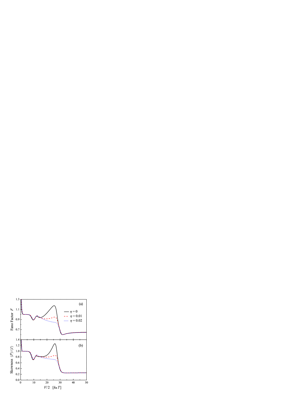
Figure 4: (A) Fano factor and (b) normalized skewness versus bias voltage for different dissipative couplings $\eta$. The tunnel couplings to the left and right electrodes are asymmetric ($\Gamma_{\rm L}=10\Gamma_{\rm R}$) and the energy cutoff for the phonon bath spectral density is $\omega_{\rm c}=5\Gamma$. The other parameters are the same as those in Fig. 2.

Finally, let us turn to the influence of external phonon bath which leads to relaxation and dephasing in the system Brandes (2005); Wang et al. (2005). The corresponding rates are given respectively by Aguado and Brandes (2004); Kießlich et al. (2007); Luo et al. (2010b)

$$\Gamma_{\pm}=-\frac{\pi}{2}\frac{\Omega}{\Delta}J_{\rm ph}(\Delta)\left[\frac{\epsilon}{\Delta}\coth\left(\frac{\Delta}{2k_{\rm B}T}\right)\pm 1\right]+\eta\pi\frac{k_{\rm B}T\Omega\epsilon}{\Delta^{2}},$$ (21a)

and

$$\gamma_{\rm ph}=2\pi\frac{\Omega^{2}}{\Delta^{2}}J_{\rm ph}(\Delta)\coth\left(\frac{\Delta}{2k_{\rm B}T}\right)+\eta\pi\frac{k_{\rm B}T\epsilon^{2}}{\Delta^{2}},$$ (21b)

where $J_{\rm ph}(\omega)=\eta\omega e^{-\omega/\omega_{{\rm c}}}$ is the Ohmic spectral density of the heat bath, with the dimensionless parameter $\eta$ reflecting the strength of dissipation and $\omega_{\rm c}$ the Ohmic high energy cutoff.

The calculated Fano factor and normalized skewness versus bias voltage are plotted in Fig. 4 for different dissipative couplings $\eta$. Strong suppression of the cumulants is observed in the DDCB regime, where double occupation on the system is prohibited. In the absence of electron–phonon coupling, electrons are transferred coherently. The phonon bath coupling, on one hand, leads to dephasing of the quantum state, and electrons tend to be tunneled sequentially, which then causes the reduction of noise in the DDCB regime Kießlich et al. (2007). On the other hand, the involving phonon emission and absorption processes give rises to a relaxation mechanism, which further suppresses the noise. The noise suppression is particularly notable in the bias close to $\bar{E}+U^{\prime}$, where the energy renormalization is prominent, as shown by the dotted curves in Fig. 4(a) and (b) for a strong dissipative coupling $\eta=0.02$. These features demonstrate that both Fano factor and skewness are sensitive tools to the phonon bath induced dephasing and relaxation.

V Conclusion

In summary, we have investigated the full counting statistics of electron transport through double quantum dots coupled in series, and paid particular attention to the unique features arising from the level renormalization. It is found that a dynamical channel blockade mechanism is developed purely due to the energy renormalization, which eventually leads to a pronounced super–Poissonian noise. Our results demonstrate unambiguously the importance of the level renormalization when investigating the transport properties of a double dot structure. Negative differential conductance due to level detuning renormalization is observed, and its relation with the super–Poissonian noise is revealed. Coupling of the double dots to an external phonon bath leads to dephasing and relaxation mechanisms, which are shown to suppress noise notably. Furthermore, double dot systems, as recently shown in Refs. Yin et al. (2005); Emary (2009), are good candidates for entanglement generation. In this context, the present full counting statistics have the potential to facilitate the identification and characterization of entanglement originating from different sources.