Opportunistic Buffered Decode-Wait-and-Forward (OBDWF) Protocol for Mobile Wireless Relay Networks

Abstract

In this paper, we propose an opportunistic buffered decode-wait-and-forward (OBDWF) protocol to exploit both relay buffering and relay mobility to enhance the system throughput and the end-to-end packet delay under bursty arrivals. We consider a point-to-point communication link assisted by $K$ mobile relays. We illustrate that the OBDWF protocol could achieve a better throughput and delay performance compared with existing baseline systems such as the conventional dynamic decode-and-forward (DDF) and amplified-and-forward (AF) protocol. In addition to simulation performance, we also derived closed-form asymptotic throughput and delay expressions of the OBDWF protocol. Specifically, the proposed OBDWF protocol achieves an asymptotic throughput $\mathbf{\Theta}(\log_{2}K)$ with $\mathbf{\Theta}(1)$ total transmit power in the relay network. This is a significant gain compared with the best known performance in conventional protocols ($\mathbf{\Theta}(\log_{2}K)$ throughput with $\mathbf{\Theta}(K)$ total transmit power). With bursty arrivals, we show that both the stability region and average delay of the proposed OBDWF protocol can achieve order-wise performance gain $\mathbf{\Theta}(K)$ compared with conventional DDF protocol.

I Introduction

In wireless communication networks, cooperative relaying not only extends the coverage but also contributes the spatial diversity. As a result, cooperative relay is one of the core technology components in the next generation wireless systems such as IEEE 802.16m and LTE-A. There are extensive studies on the theory and algorithm design of cooperative relay, and they can be roughly classified as focusing on the microscopic and macroscopic aspects. Examples of microscopic studies include the decode-and-forward (DF), amplify-and-forward (AF) and compress-and-forward (CF) protocols for single hop [1, 2, 3] as well as multi-hop cooperative relay networks [4]. In [5], the authors demonstrated that AF could achieve optimal end-to-end DoF for the MIMO point-to-point system with multiple relay nodes. In [6], it is shown that a variant of the CF relaying achieves the capacity of any general multi-antenna Gaussian relay network within a constant number of bit. In [7], relay selection protocol is shown to achieve higher bandwidth efficiency while guaranteeing the same diversity order as that of the conventional cooperative protocols. However, all these works have focused on the physical layer performance (such as throughput) and failed to exploit the buffer dynamics in the relay. Furthermore, they have assumed all the relays are static and have ignored the potential benefit introduced by mobility in the network. On the other hand, there are also some papers focusing on studying the macroscopic behavior of cooperative ad-hoc networks. For example, the scaling law of the wireless ad-hoc network is derived in [8, 9, 10, 11] and it is shown that each node can achieve the throughput of the order $O(\frac{1}{\sqrt{K\log_{2}K}})$ when $K$ fixed nodes are randomly distributed over a unit area. These results imply that the throughput of each node converges to zero when the number of nodes increases. Nevertheless, it is found in [12] that the per-node throughput can arbitrarily close to constant by hierarchical cooperation. In [13, 14], it's shown that the source-destination throughput can scale as $\mathbf{\Theta}(\log_{2}K)$ when all the relays amplify and forward the received packet to the destination cooperatively with $\mathbf{\Theta}(K)$ total transmission power. In [15], the authors have shown that a per link throughput of $\mathbf{\Theta}(1)$ can be achieved at the expense of potentially large delay when the nodes are mobile. All these works have suggested that there are potential advantage of relay buffering and relay mobility. However, there are also various technical challenges to be addressed before we could better understand the potential benefits.

• Low Complexity Relay Protocol Design Exploiting Relay Buffering and Relay Mobility: Although the idea of utilizing the mobility has been studied in [15, 16] in the study of ad-hoc network throughput analysis (scaling laws), there is not much work that addresses the microscopic details (such as protocol design) of the problem. For example, most of the existing relay protocols have focused entirely on the physical layer performance (information theoretical capacity or Degrees-of-Freedom (DoF)) and they did not fully exploit the potential of relay buffering. In fact, it is quite challenging to design low complexity relay protocol that could exploit both the relay buffering and relay mobility. Furthermore, the issue is further complicated by the bursty source arrival and randomly coupled queue dynamics in the systems.

• Performance Analysis: It is very important to have closed form performance analysis to obtain insights to understand the fundamental tradeoff between throughput gain and delay penalty in cooperative systems. However, it is very challenging to analyze closed form tradeoff between the throughput, stability region and end-to-end delay. For instance, most of the existing papers studying delay and throughput scaling laws in ad-hoc network [15, 16] are focused on the macroscopic aspects of the systems and they have ignored the microscopic details such as the random bursty arrivals and queue dynamics in the systems. When these dynamics are taken into consideration, the problem involves both information theory (to model the physical layer dynamics) and the queueing theory (to model the queue dynamics), which is highly non-trivial.

In this paper, we shall propose an opportunistic buffered decode-wait-and-forward (OBDWF) protocol to exploit both relay buffering and relay mobility to enhance the system throughput and the end-to-end packet delay under bursty arrivals. We consider a point-to-point communication link assisted by $K$ mobile relays. By exploiting the relay buffering and relay mobility in the phase I and phase II of the proposed OBDWF, we shall illustrate that the OBDWF could achieve a better throughput and delay performance compared with existing baseline systems such as the conventional Dynamic Decode-and-Forward (DDF) [3] and AF protocol [17]. In addition to simulation performance, we also derived closed-form asymptotic throughput and delay expressions of the OBDWF protocol. Under random bursty arrivals and queue dynamics, the proposed OBDWF protocol has low complexity with only $O(K)$ communication overhead and $\mathbf{\Theta}(1)$ total transmit power in the relay network. It achieves a throughput $\mathbf{\Theta}(\log_{2}K)$, which is a significant gain compared with the best known performance in conventional protocols ($\mathbf{\Theta}(\log_{2}K)$ throughput with $\mathbf{\Theta}(K)$ total transmit power). Furthermore, both the stability region and average delay can achieve order-wise performance gain $\mathbf{\Theta}(K)$ compared with conventional DDF protocol.

II System Model

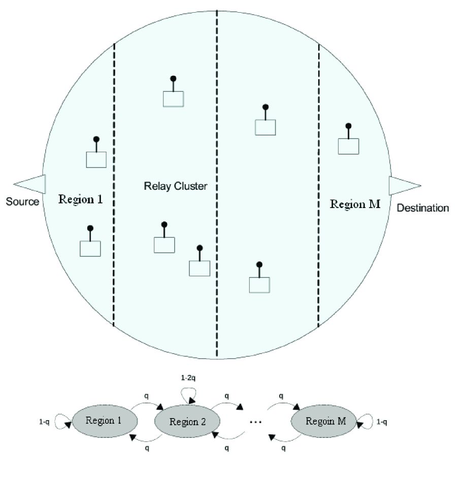
Figure 1: System and random walk mobility model for the point-to-point communication system with a half-duplexing mobile relay network. The parameter $q$ determines the mobility of the network (larger $q$ means higher mobility).

In this section, we shall describe the system model for the point-to-point communication system with a half-duplexing mobile relay network. Specifically, there are $K$ mobile relay nodes between the source node and the destination node, as shown in Fig. 1. Each of the source node and the $K$ relay nodes has an infinite length buffer. To facilitate the relay scheduling, transmission is partitioned into frames. Each frame is further divided into three types of slots defined as follows:

• Channel Estimation Slot is used by relays for estimating the channel gains with the source and destination nodes.

• Control Slot is used by relays for distributive control signaling of the OBDWF protocol. The details is given in the protocol description.

• Transmission Slot is used for data transmission, and it last $\tau$ seconds.

II-A Relay Mobility Model

Following [8, 14], we assume that the $K$ relays are distributed on a disk with radius $R$ as illustrated in Fig. 1. The source and the destination nodes are fixed at two ends of a diameter, and the disk is divided horizontally into $M$ equal-area regions along the source-destination diameter. These regions are denoted as region 1, region 2, …, and region $M$, from the source to the destination. As illustrated in Fig. 1, the movement of each relay is modeled as a random walk (Markov chain) over these regions:

• At the beginning, each relay is uniformly distributed on the disk. Movements of relays can only occur in discrete frames with time index $t$.

• Let $X_{k}(t)$ denote the region index of the $k$-th relay in the $t$-th frame, $\{X_{k}(t)|t=1,...+\infty\}$ is a Markov chain with the following transition matrix

  $$\begin{array}[]{l}\Pr\{X_{k}(t+1)|X_{k}(t)\}=\\ \left\{\begin{array}[]{ll}q&X_{k}(t+1)=X_{k}(t)\pm 1\\ 1-2q&X_{k}(t+1)=X_{k}(t)=2,...,M-1\\ 1-q&X_{k}(t+1)=X_{k}(t)=1\mbox{ or }M\\ 0&\mbox{ otherwise }\end{array}\right.\end{array}$$ (1)

• When one relay moves into a region, its actual location in this region is uniformly distributed.

Remark 1 (Interpretation of Parameter $q$)

The region transition probability $q\in(0,\frac{1}{2}]$ measures how likely one relay will move into another region in the next frame, and therefore, it is related to the average speed of the relays.   ∎

II-B Physical Layer Model

Let $H_{s,j}$ and $d_{s,j}$ be the small scale fading gain and the distance between the source node and the $j$-th relay respectively, and let $H_{j,d}$ and $d_{j,d}$ be the small scale fading gain and the distance between the $j$-th relay and destination node respectively.

Assumption 1 (Assumption on the Channel Model)

We assume that $\{H_{s,j},H_{j,d}\}$ are quasi static in each frame. Furthermore, $\{H_{s,j},H_{j,d}\}$ are i.i.d over frames according to a general distribution $\Pr\{H\}$ and independent between each link.   ∎

The relay network shares a common spectrum with bandwidth $W$Hz, and each node transmits at a peak power $P$. Let $x_{s}$ be the transmitted symbol from the source node, the received signal at the $j$-th relay is given by: $y_{j}=\sqrt{H_{s,j}/{d_{s,j}^{\alpha}}}x_{s}+z_{j}$, where $\alpha$ is the path loss exponent, and $z_{j}$ is the i.i.d $\mathcal{N}(0,1)$ noise. The achievable data rate between the source node and the $j$-th relay is given by:

$$C_{s,j}=W\log_{2}(1+P\xi H_{s,j}/{d_{s,j}^{\alpha}}),$$ (2)

where $\xi\in(0,1]$ is a constant can be used to model both the coded and uncoded systems. Similarly, the achievable data rate between $j$-th relay and the destination node is given by

$$C_{j,d}=W\log_{2}(1+P\xi H_{j,d}/{d_{j,d}^{\alpha}}),$$ (3)

All the packets are transmitted at data rate $R=W\log_{2}\beta$ for some constant $\beta$. The $j$-th relay could correctly decode the packets transmitted from the source node if $R\leq C_{s,j}$, and the destination node could correctly decode the packets transmitted from the $j$-th relay if $R\leq C_{j,d}$. For easy discussion, we shall denote a link as a connected link if its achievable data rate is larger than $R$, and otherwise a broken link.

III The OBDWF Protocol

In this section, we shall first describe the proposed opportunistic buffered decode-wait-and-forward (OBDWF) relay protocol for mobile relays.

Protocol 1 (OBDWF Protocol for Mobile Relays)

• Each relay measures the current states {connected, broken} of its links with the destination node in the channel estimation slot.

• The control slot is divided into mini-slots. If the buffer in a relay is not empty and the link state to the destination is connected, it will submit a request in a control mini-slot. Using standard contention mechanism, one active relay is selected to transmit its packet from its buffer to the destination node. The selected relay as well as all the other relays will dequeue the same packet from their buffers.

• If none of the $K$ relays attempts to compete for access to the destination node in the control slot, the source node will broadcast a new packet to the $K$ relays and the destination node using a fixed data rate $R=W\log_{2}\beta$ for some constant $\beta$. The source node will dequeue the packet from its buffer if there is an ACK from at least one of the relays or the destination node.   ∎

Note that the OBDWF protocol has only $O(K)$ communication overhead with $\mathbf{\Theta}(1)$ total transmit power in the relay network, which is the same as the conventional DDF and conventional AF protocol, elaborated in Table I. Unlike conventional DDF protocol where the phase I (source to relay) and the phase II (relay to destination) of the same packet appear as inseparable atomic actions, the proposed OBDWF protocol exploits buffers in the relays to create the flexibility to schedule phase I and phase II of the same packet based on the instantaneous channel state as illustrated in Fig. 2. Coupled with relay mobility, the proposed OBDWF protocol allows the relay to buffer the packet and wait for good opportunity (when the relays is close to the destination) to deliver the packet. As a result, relay mobility allows the system to operate at a higher throughput at the expense of larger delay. We shall quantify such tradeoff in Section IV and V.

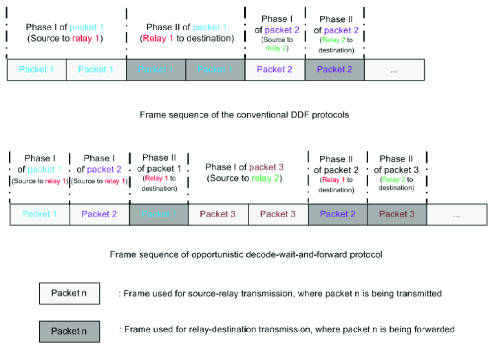
Figure 2: Frame sequences for conventional DDF protocl and opportunistic buffered decode-wait-and-forward (OBDWF) protocol. In conventional DDF protocol, the phase I and the phase II of the same packet appear as inseparable atomic actions. On the other hand, the proposed OBDWF protocol exploits buffers in the relays to create the flexibility to schedule phase I and phase II of the same packet based on the instantaneous channel state. Coupled with relay mobility, the proposed OBDWF protocol allows the relay to buffer the packet and wait for good opportunity (when the relays is close to the destination) to deliver the packet.

IV Throughput Performance with Infinite Backlog

In this section, we shall first discuss the average system throughput of the proposed OBDWF protocol with infinite backlog at the source buffer. We first define the average throughput below.

Definition 1 (Average End-to-End System Throughput)

Let $T_{i}$ be the number of information bits successfully received by the destination node at the $i$-th frame. The average end-to-end system throughput between the source node and the destination node $\overline{T}$ is defined as $\overline{T}=\lim_{\kappa\rightarrow\infty}\frac{\sum_{i=1}^{\kappa}T_{i}}{\kappa\tau}$.   ∎

IV-A Throughput Performance of the OBDWF Protocol

Note that for a fixed number of relay nodes $K$, when the source node increases the data rate $R$, the associate radio coverage and the number of relays who can decode the source packet becomes smaller. On the other hand, for fixed $R$, the number of relays who can decode the source packet increases as $K$ increases. We shall quantify such scaling relationship in Lemma 1.

Lemma 1 (Scaling Relationship of Connected Link)

Denote the transmit data rate $R=W\log_{2}\beta$ and $\gamma=\beta^{\frac{2}{\alpha}}$ for some constant $\beta$. For sufficiently large $K$, the following statements are true:

• I. If $\lim\limits_{K\rightarrow\infty}\frac{\gamma}{K}=0$, the probability that there are $\mathbf{\Theta}(\frac{K}{\gamma})$ relays having connected links with the source node (or the destination node) tends to $1$.

• II. If $\lim\limits_{K\rightarrow\infty}\frac{\gamma}{K}>0$, the probability that there are $\mathbf{\Theta}(1)$ relays having connected links with the source node (or the destination node) is $\mathbf{\Theta}(\frac{K}{\gamma})$.   ∎

Proof:

Please refer to Appendix A. ∎

Using Lemma 1, we obtain the closed-form asymptotic average system throughput under infinite backlog at the source buffer.

Theorem 1

(Throughput Performance of the OBDWF Protocol): For sufficiently large $K$ and infinite backlog at the source buffer, the maximal average system throughput of the proposed OBDWF protocol under the random walk mobility model in (1) is given by

$$\overline{T}^{*}_{\text{OBDWF}}=\mathbf{\Theta}(\log_{2}K)$$ (4)

This order-wise throughput is achieved when $\gamma=\mathbf{\Theta}(K^{\sigma})$ for some constant $\sigma\in(0,1]$. Furthermore, $\overline{T}^{*}_{\text{OBDWF}}$ is upper-bounded by but infinitely close to $\frac{W\alpha}{4}\log_{2}K$.   ∎

Proof:

Please refer to Appendix B. ∎

Remark 2 (Interpretation of Theorem 1)

Since there are infinitely large buffers at the relay nodes and the random-walk transition probability $q$ is positive, the average system throughput is $R/2$ as long as there are always relays having connected links to the source and destination node (which is presented mathematically as $\lim\limits_{K\rightarrow\infty}\frac{\gamma}{K}=0$ by Lemma 1).   ∎

IV-B Comparison with the Conventional DDF Protocol

Similarly, we shall summarize the closed-form asymptotic average system throughput for the conventional DDF protocol ( elaborated in Table I) below.

Lemma 2

(Throughput Performance of Conventional DDF Protocol): For sufficiently large $K$ and infinite backlog at the source buffer, the maximal average system throughput of the conventional DDF protocol under the random walk mobility model in (1) is given by:

$$\overline{T}^{*}_{\text{DDF}}=\min\left\{\mathbf{\Theta}((Kq^{M-1})^{1/M}),\mathbf{\Theta}\left(\log_{2}(Kq^{M-1})\right)\right\}$$ (5)

This order-wise throughput is achieved when

$$\gamma=\max\left\{\mathbf{\Theta}(1),\mathbf{\Theta}(\sqrt{Kq^{M-1}})\right\}$$ (6)

Proof:

Please refer to the Appendix C. ∎

Therefore, we have the following corollary on the performance gain of the OBDWF protocol:

Corollary 1

(Comparison of the Average System Throughput): The throughput gain of the OBDWF protocol is

$$\frac{\overline{T}^{*}_{\text{OBDWF}}}{\overline{T}^{*}_{\text{DDF}}}=\left\{\begin{array}[]{ll}\mathbf{\Theta}\left(\frac{\log_{2}K}{\log_{2}(Kq^{M-1})}\right)&\text{if }\lim\limits_{K\rightarrow\infty}Kq^{M-1}=\infty\\ \mathbf{\Theta}\left(\frac{\log_{2}K}{(Kq^{M-1})^{1/M}}\right)&\text{otherwise}\end{array}\right.$$ (7)

Remark 3 (Interpretation of Corollary 1)

Note that when the system mobility is low ($q=(\frac{\log_{2}K}{K})^{\frac{1}{M-1}}$), there is an order-wise throughput gain achieved by the OBDWF protocol.   ∎

V Stability and Delay Performance with Bursty Arrivals

In this section, we shall focus on the stability region and the delay performance analysis of the proposed OBDWF protocol under bursty packet arrivals. We shall first define the busty source model, followed by the analysis on the stability region and average delay performance.

V-A Bursty Source Model

Let $A_{s}(t)$ represents the number of new packets arriving at the source node at the beginning of the $t$-th frame.

Definition 2 (Bursty Source Model)

We assume that the arrival process $A_{s}(t)$ is i.i.d over the frame index $t$ according to a general distribution $\Pr\{A_{s}\}$. Each new packet has a fixed number of bits $\overline{N}$. The first and second order moments of the arrival process are denoted by $\lambda_{s}=\mathbb{E}[A_{s}]$ and $\lambda_{s}^{(2)}=\mathbb{E}[A_{s}^{2}]$ respectively.   ∎

Let $Q_{s}(t)$ be the number of packets in the source buffer at the $t$-th frame. The dynamics of the source buffer state is given by:

$$Q_{s}(t+1)=A_{s}(t+1)+\left[Q_{s}(t)-U_{s}(t)\right]^{+}$$ (8)

where $U_{s}(t)\in\{0,1\}$ is the number of packets transmitted to the relay network at $t$-th frame. Furthermore, let $Q_{k}(t)$ be the number of packets in the the $k$-th relay node's buffer at the $t$-th frame. The dynamics of the relay buffer state is given by:

$$Q_{k}(t+1)=A_{k}(t+1)+\left[Q_{k}(t)-U_{k}(t)\right]^{+}$$ (9)

where $A_{k}(t)\in\{0,1\}$ is the number of packets received by the $k$-th relay node from the source node at the beginning of the $t$-th frame, and $U_{k}(t)\in\{0,1\}$ is the number of packets dequeued from the $k$-th relay node at the $t$-th frame.

V-B Stability Performance

In this section, we shall derive the stability region of the OBDWF protocol and the conventional DDF protocols. We first define the notion of queue stability [18, 19] below.

Definition 3 (Stability of the Queueing System)

The queueing system is stable, if

$$\lim_{t\rightarrow\infty}\Pr\{Q(t)<x\}=F(x)\text{ and }\lim_{x\rightarrow\infty}F(x)=1$$ (10)

where $Q(t)$ is the queue state in the queueing system at the $t$-th frame.   ∎

Using Definition 3, we have the following Theorem for the OBDWF protocol.

Theorem 2 (Stability Region of the OBDWF Protocol)

For sufficiently large $K$, the system of queues $\{Q_{s}(t),Q_{1}(t),\cdots,Q_{K}(t)\}$ under the proposed OBDWF protocol are stable if and only if $\lambda_{s}<\frac{1}{\zeta}$, where $\zeta$ is given by

$$\zeta=\max\left\{\mathbf{\Theta}(1),\mathbf{\Theta}(\gamma/{K})\right\}$$ (11)

Proof:

Please refer to Appendix E. ∎

Similarly, the stability region of the conventional DDF protocol is given by:

Lemma 3 (Stability Region of the Conventional DDF Protocol)

For sufficiently large $K$, the system of queues $\{Q_{s}(t),Q_{1}(t),\cdots,Q_{K}(t)\}$ under conventional DDF protocol are stable if and only if $\lambda_{s}<\frac{1}{\overline{D}_{S}}$, where $\overline{D}_{S}$ is given by

$$\begin{array}[]{l}\overline{D}_{S}=\\ \left\{\begin{array}[]{ll}\begin{array}[]{l}\max\big{\{}\mathbf{\Theta}(1),\\ \mathbf{\Theta}\big{[}(\frac{\gamma^{2}}{Kq^{M-1}})^{\frac{1}{M}}\big{]}\big{\}}\end{array}&\text{If }\lim\limits_{K\rightarrow\infty}\frac{\gamma}{K}=0\text{ and }\lim\limits_{K\rightarrow\infty}\frac{K}{q\gamma^{2}}>0\\ \mathbf{\Theta}(\frac{\gamma^{2}}{K})&\text{If }\lim\limits_{K\rightarrow\infty}\frac{\gamma}{K}=0\text{ and }\lim\limits_{K\rightarrow\infty}\frac{K}{q\gamma^{2}}=0\\ \mathbf{\Theta}\left[\left(\gamma/q^{M-1}\right)^{\frac{1}{M}}\right]&\text{If }\lim\limits_{K\rightarrow\infty}\frac{\gamma}{K}>0\text{ and }\lim\limits_{K\rightarrow\infty}\frac{1}{q\gamma}>0\\ \mathbf{\Theta}(\gamma)&\text{If }\lim\limits_{K\rightarrow\infty}\frac{\gamma}{K}>0\text{ and }\lim\limits_{K\rightarrow\infty}\frac{1}{q\gamma}=0\end{array}\right.\end{array}$$ (12)

Proof:

Using Lemma 5 in Appendix C, the results in Lemma 3 follows using similar argument as in Appendix E. ∎

The following Corollary summarizes the performance gain of the OBDWF protocol in stability region.

Corollary 2 (Stability Region Comparison)

Let $\lambda_{s}^{*}(\text{OBDWF})$ and $\lambda_{s}^{*}(\text{DDF})$ be the maximum source arrival rate the system can support and maintain queue stability using OBDWF and conventional DDF protocol respectively. For sufficiently large $K$, the gain on the stability region is given by:

$$\begin{array}[]{l}\frac{\lambda_{s}^{*}(\text{OBDWF})}{\lambda_{s}^{*}(\text{DDF})}=\\ \left\{\begin{array}[]{ll}\begin{array}[]{l}\max\big{\{}\mathbf{\Theta}(1),\\ \mathbf{\Theta}\big{[}(\frac{\gamma^{2}}{Kq^{M-1}})^{\frac{1}{M}}\big{]}\big{\}}\end{array}&\text{If }\lim\limits_{K\rightarrow\infty}\frac{\gamma}{K}=0\text{ and }\lim\limits_{K\rightarrow\infty}\frac{K}{q\gamma^{2}}>0\\ \mathbf{\Theta}(\frac{\gamma^{2}}{K})&\text{If }\lim\limits_{K\rightarrow\infty}\frac{\gamma}{K}=0\text{ and }\lim\limits_{K\rightarrow\infty}\frac{K}{q\gamma^{2}}=0\\ \mathbf{\Theta}\left(K(\gamma q)^{\frac{1-M}{M}}\right)&\text{If }\lim\limits_{K\rightarrow\infty}\frac{\gamma}{K}>0\text{ and }\lim\limits_{K\rightarrow\infty}\frac{1}{q\gamma}>0\\ \mathbf{\Theta}(K)&\text{If }\lim\limits_{K\rightarrow\infty}\frac{\gamma}{K}>0\text{ and }\lim\limits_{K\rightarrow\infty}\frac{1}{q\gamma}=0\end{array}\right.\end{array}$$ (13)

Remark 4 (Interpretation of the Corollary 2)

Note that when the packet size $\overline{N}$ is large such that $\gamma>\mathbf{\Theta}(\psi)$, then the OBDWF protocol can obtain an order-wise gain. For example, when $\gamma=\mathbf{\Theta}(K)$ and $q=\mathbf{\Theta}(1)$, then $\frac{\lambda_{s}^{*}(\text{OBDWF})}{\lambda_{s}^{*}(\text{DDF})}=\mathbf{\Theta}(K)$.   ∎

V-C Delay Performance

In this section, we shall compare the average end-to-end packet delay performance. The average end-to-end packet delay of the relay network is defined below.

Definition 4 (Average End-to-End Packet Delay)

Let $I_{i}^{a}$ and $I_{i}^{r}$ be the frame indices of the $i$-th packet arrival at the source node and the $i$-th packet successfully received at the destination node respectively. The average end-to-end packet delay of the relay network is defined as $\overline{D}=\lim_{\kappa\rightarrow\infty}\frac{\sum_{i=1}^{\kappa}I_{i}^{r}-I_{i}^{a}}{\kappa}$.   ∎

The following Theorem summarizes the average delay performance of the proposed OBDWF protocol.

Theorem 3

(Average End-to-End Packet Delay of the OBDWF Protocol): For sufficiently large $K$ and $\lambda_{s}$ in the stability region in Theorem 2, the average end-to-end packet delay of the OBDWF protocol is given by:

$$\overline{D}_{\text{OBDWF}}=\max\left\{\mathbf{\Theta}\left(\frac{\lambda_{s}^{(2)}\zeta}{\lambda_{s}(1-\lambda_{s}\zeta)}\right),\mathbf{\Theta}(\overline{D}_{S})\right\}$$ (14)

where $\zeta$ is given by (11) and $\overline{D}_{S}$ is given by (12).   ∎

Proof:

Please refer to Appendix F. ∎

Remark 5 (Interpretation of Theorem 3)

The first term in the RHS of (14) is the average waiting time (number of frames) that the packets stays in the source buffer. It is affected by the source arrival model, i.e., $\lambda_{s}$ and $\lambda_{s}^{(2)}$. The second term $\overline{D}_{S}=\mathbf{\Theta}(\overline{D}_{R})$, where $\overline{D}_{R}$ is the average time the packet stays in the relay network. This factor depends on both the packet size $\overline{N}$ and the mobility of the network ($q$). Fig. 3 further illustrates the asymptotic relationship between $\overline{D}_{S}$, $\gamma$ and $q$. Specifically, the x-axis is $\frac{\log\gamma}{\log K}$, and the y-axis is $\frac{\log\overline{D}_{S}}{\log K}$. Observe that $\overline{D}_{S}$ is an increasing function of $\gamma$ and $1/q$.   ∎

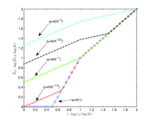
Figure 3: The asymptotic relationship between $\overline{D}_{S}$, $\gamma$ and $q$. Specifically, the x-axis is $\frac{\log(\gamma)}{\log(K)}$, and the y-axis is $\frac{\log(\overline{D}_{S})}{\log(K)}$.

Similarly, the delay performance of the conventional DDF protocol is summarized in the following Lemma:

Lemma 4

(Average End-to-End Packet Delay of the Conventional DDF Protocol): For sufficiently large $K$ and $\lambda_{s}$ in the stability region in Lemma 3, the average end-to-end packet delay under the conventional DDF protocol is given by:

$$\overline{D}_{\text{DDF}}=\mathbf{\Theta}\left(\frac{\lambda_{s}^{(2)}\overline{D}_{S}}{\lambda_{s}(1-\lambda_{s}\overline{D}_{S})}\right)$$ (15)

where $\overline{D}_{S}$ is given by (12).   ∎

Proof:

Please refer to the Appendix G. ∎

The following Corollary summarizes the average delay gain of the OBDWF protocol.

Corollary 3 (Average Delay Comparison)

For sufficiently large $K$ and $\lambda_{s}$ in the stability region in Lemma 3, the average delay gain of the OBDWF and the conventional DDF protocols is given by:

$$\begin{array}[]{l}\frac{\overline{D}_{\text{DDF}}}{\overline{D}_{\text{OBDWF}}}=\\ \quad\quad\min\left\{\mathbf{\Theta}\left(\frac{\lambda_{s}^{(2)}}{\lambda_{s}(1-\lambda_{s}\overline{D}_{S})}\right),\mathbf{\Theta}\left(\frac{\overline{D}_{S}(1-\lambda_{s}\zeta)}{\zeta(1-\lambda_{s}\overline{D}_{S})}\right)\right\}\end{array}$$ (16)

where $\zeta$ is given by (11) and $\mathbf{\Theta}(\overline{D}_{S})$ is given by (12).   ∎

Remark 6 (Interpretation of the Corollary 3)

There are several scenarios that the OBDWF protocol will have significant order-wise gain on the delay performance. For example, when $\lambda_{s}$ is close to the service rate $1/\overline{D}_{S}$, i.e., $\lambda_{s}=\frac{1}{\overline{D}_{S}}-\epsilon$ where $\epsilon=o(\frac{1}{\overline{D}_{S}})$, we have $\frac{\overline{D}_{\text{DDF}}}{\overline{D}_{\text{OBDWF}}}=\mathbf{\Theta}(\frac{1}{\epsilon\overline{D}_{S}})>\mathbf{\Theta}(1)$. On the other hand, even if $\lambda_{s}$ is not so close to $\frac{1}{\overline{D}_{S}}$, i.e., $1-\lambda_{s}\overline{D}_{S}=\mathbf{\Theta}(1)$, there will still be order-wise gain as long as $\frac{\lambda_{s}}{\lambda_{s}^{(2)}}=o(1)$ and $\frac{1}{\overline{D}_{S}}=o(1)$. Specifically, if $\Pr\{A_{s}(t)=\mathbf{\Theta}(K)\}=\nu$, $\Pr\{A_{s}(t)=0\}=1-\nu$, where $\nu=\mathbf{\Theta}(\frac{1}{K^{2}})$, $\gamma=\mathbf{\Theta}(K)$ and $q=\mathbf{\Theta}(1)$, then we can obtain $\frac{\overline{D}_{\text{DDF}}}{\overline{D}_{\text{OBDWF}}}=\mathbf{\Theta}(K)$ by (16).   ∎

VI Simulation Results and Discussion

TABLE I: Elaboration of the baselines. Specifically, baseline 1 refers to conventional DDF protocol[3], baseline 2 refers to conventional AF protocol[17], baseline 3 refers to AF with spatial combining and baseline 4 refers to DF with Spatial Combining.

Baseline Name	Description
Baseline 1 (Conventional DDF)	$\bullet$ The source node broadcasts a packet from the buffer at the beginning of the frame until at least one relay or destination node returns with an ACK. $\bullet$ If the destination node returns with an ACK, the source node start to broadcast a new packet; If the relay node returns with an ACK, the source node stops broadcasting and the relay node forward the packet to the destination node in the next frame.
Baseline 2 (Conventional AF)	$\bullet$ The source node broadcasts a packet from the buffer at the beginning of a frame. $\bullet$ All the relays listen and store the received samples from the source during the listening phase and the relay with the largest metric ($\frac{P^{2}S_{s,j}S_{j,d}}{PS_{s,j}+PS_{j,d}+1}$, where $S_{s,j}=\frac{H_{s,j}}{d_{s,j}^{\alpha}}$ and $S_{j,d}=\frac{H_{j,d}}{d_{j,d}^{\alpha}}$ ) is selected to amplify and forward to the destination node in the next frame.
Baseline 3 (AF with Spatial Combining)	$\bullet$ The source node broadcasts a packet from the buffer at the beginning of a frame. $\bullet$ All the relays listen and store the received samples from the source during the listening phase and $N_{A}$ relays with the largest metric ($\frac{P^{2}S_{s,j}S_{j,d}}{PS_{s,j}+PS_{j,d}+1}$, where $S_{s,j}=\frac{H_{s,j}}{d_{s,j}^{\alpha}}$ and $S_{j,d}=\frac{H_{j,d}}{d_{j,d}^{\alpha}}$ ) are selected to amplify and forward to the destination node in the next frame.
Baseline 4 (DF with Spatial Combining)	$\bullet$ The source node broadcasts a packet from the buffer at the beginning of the frame until at least $N_{D}$ relay nodes or destination node return with an ACK. $\bullet$ If the destination node returns with an ACK, the source node starts to broadcast a new packet; If at least $N_{D}$ relay nodes return with an ACK, the source node stops broadcasting and all the relay nodes that have decoded the packet from the source node will forward the packet to the destination node in the next frame.

In this section, we shall compare the performance of the proposed OBDWF protocol with various baseline schemes. Baseline 1 refers to the conventional DDF protocol[3], baseline 2 refers to the conventional AF protocol[17]. Baseline 3 and 4 are extensions of Baseline 1 and 2 respectively with spatial combining from multiple relays, which are elaborated in Table I We consider a system with the source node at $(0,0)$ and the destination node at $(5,0)$. The $K$ relays are randomly distributed between the source node and the destination node, as shown in Fig. 1. The movement of each relay is given by the random walk mobility model in (1), where the number of relay mobility regions is $M=5$. The small scale fading gain follows complex Guassian with unit variance. The pass loss exponent $\alpha=4$, and the transmit SNR $P=20$dB. For bursty arrivals, we assume $\Pr\{A_{s}=15\}=0.001$ and $\Pr\{A_{s}=0\}=0.999$. This corresponds to an arrival rate $\lambda_{s}=0.015$. The packet size $\overline{N}=W\tau\log_{2}K$, the frame duration $\tau=5$ ms and the bandwidth $W=1$MHz. Using Lemma 2, the physical data rate at the source node is set to be $R=W\log_{2}K$, which is the optimal choice for conventional DDF.

Fig. 4 illustrates the average end-to-end system throughput $\overline{T}$ versus the number of relays $K$ at different mobility $q$. Observe that the proposed OBDWF protocol has significant gain compared with the baselines. Furthermore, the performance of the OBDWF protocol is insensitive to the mobility of the network $q$. Fig. 5 illustrates the maximal stable arrival rate $\lambda_{s}$ versus the number of relays $K$ at different network mobility $q$ under the bursty source model. Similar significant gains over the baselines can be observed. Moreover, it can be observed in these two figures that the simulation results match with the theoretical results derived in Section IV and V.

Fig. 6 illustrates the average end-to-end packet delay versus the number of relays $K$ at different mobility $q$ with finite buffer length of 25 packets for all the nodes. Note that, the delay performance is an increasing function of $1/q$ for all protocols and there is also a significant gain of the proposed OBDWF protocol.

Fig. 7 illustrates the average end-to-end packet delay versus the average arrival rate $\lambda_{s}$ with infinite buffer length for all the nodes. Note that the baseline 2 and 3 are not stable under the operating regime considered. The delay performance of baseline 4 quickly blows up at $\lambda_{s}=0.08$, which is the maximal stability input rate for this baseline. On the other hand, the delay performance of the proposed OBDWF protocol significantly out-performs all the baseline over the entire range of traffic loading. Fig. 8 illustrates the average end-to-end system throughput $\overline{T}$ versus the number of relays $K$ under the Random Waypoint Model, which is also widely used in [20, 21, 22]. Similar performance gains can be observed.

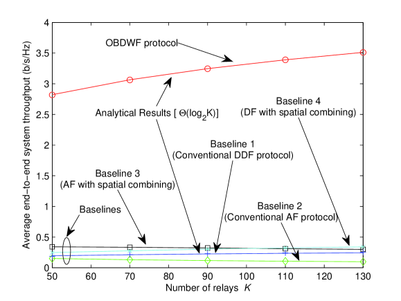
(a) $q=1/10$

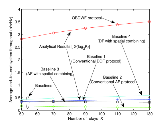
(b) $q=1/5$

Figure 4: Average end-to-end system throughput $\overline{T}$ versus the number of relays $K$ at different mobility $q$. The physical data rate is $R=W\log_{2}K$ according to Lemma 2, $(N_{A},N_{D})=(5,5)$ in the baseline 3 and 4 respectively. The marks ``o,x,+,$\square,\diamond$'' denote simulation results and the solid lines represent the analytical results for OBDWF and baseline 1 (conventional DDF) protocol.

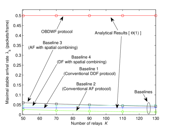
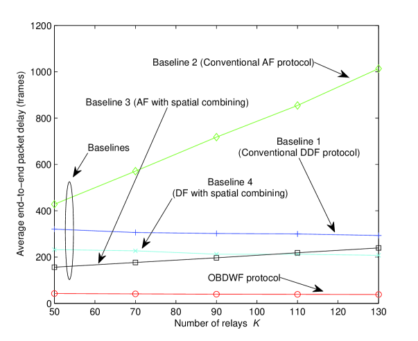
(a) $q=1/10$

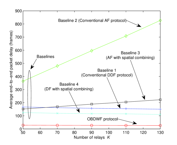
(b) $q=1/5$

Figure 5: The maximal stable arrival rate $\lambda_{s}$ versus the number of relays $K$ at different mobility $q$. The packet size is $\overline{N}=W\tau\log_{2}K$, $(N_{A},N_{D})=(5,5)$ in the baseline 3 and 4 respectively. The marks ``o,x,+,$\square,\diamond$'' denote simulation results and the solid lines represent the analytical results for OBDWF and baseline 1 (conventional DDF) protocol.

(a) $q=1/10$

(b) $q=1/5$

Figure 6: The average end-to-end packet delay versus the number of relays $K$ at different mobility $q$ with finite buffer length of 25 packets for all the nodes. The packet size is $\overline{N}=W\tau\log_{2}K$, $(N_{A},N_{D})=(5,5)$ in the baseline 3 and 4 respectively. The source arrival model is given by $\Pr\{A_{s}=15\}=0.001$ and $\Pr\{A_{s}=0\}=0.999$.

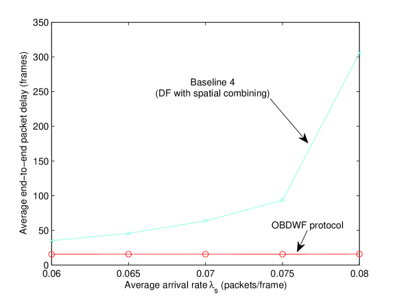
Figure 7: The average end-to-end packet delay versus the average arrival rate $\lambda_{s}$. Note that the other baselines are not stable under the operating regime considered. The packet size is $\overline{N}=W\tau\log_{2}K$, $K=110$, $q=1/5$ and $N_{D}=5$ in the baseline 4. The source arrival model is given by $\Pr\{A_{s}=1\}=\lambda_{s}$, and $\Pr\{A_{s}=0\}=1-\lambda_{s}$.

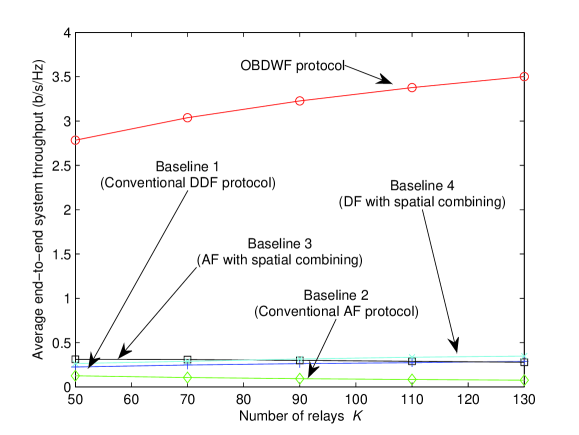
Figure 8: Average end-to-end system throughput $\overline{T}$ versus the number of relays $K$ under the random waypoint model [20, 21, 22]. Specifically, a node chooses a random destination distributed uniformly in the coverage area and moves in that direction with a random speed chosen uniformly in the interval [0.1, 0.6] (per frame). On reaching the destination the node pauses for some random time chosen uniformly in the set {0,1,$\cdots$,10} (frames) and the process repeats itself. The physical data rate is $R=W\log_{2}K$, $(N_{A},N_{D})=(5,5)$ in the baseline 3 and 4 respectively.

VII Conclusions

In this paper, we propose an opportunistic buffered decode-wait-and-forward (OBDWF) protocol for a point-to-point communication system with $K$ mobile relays. Unlike conventional DDF protocol, the proposed OBDWF protocol exploits both the relay buffering and relay mobility in the systems. We derive closed-form expressions on the asymptotic system throughput under infinite backlog as well as the average end-to-end delay under a general bursty arrival model, Based on the analysis, we found that there exists a throughput delay tradeoff in the buffered relay network. The system can achieve a higher throughput $\mathbf{\Theta}(\log_{2}K)$ using the proposed OBDWF protocol at the expense of extra delay. The system mobility affects the tradeoff as below:

• Effect on the Throughput/Stability Region Performance: According to Theorem 1, the maximal average system throughput of the proposed OBDWF protocol $\mathbf{\Theta}(\log_{2}K)$ is not influenced by the relay mobility.

• Effect on the Delay Performance: If the movement of the mobility is fast (large region transition probability $q$), the chance one relay with source's packet gets close to the destination is high, leading to small delay in the relay network, and vice versa. This can be observed from Theorem 3.

Finally, theoretical and numerical results demonstrate the significant performance gains of the proposed OBDWF protocol against various baseline references.

Appendix A: The Proof of Lemma 1

Without loss of generality, we only study the number of connected links with the source. The connection with the destination can follow the same approach.

For a given small scale fading realization $H_{s,j}$, the coverage radius of the source within which the relays have connected links to the source is given by $d=(P\xi H_{s,j})^{\frac{1}{\alpha}}/(\beta-1)^{\frac{1}{\alpha}}$. Therefore, the area of the source's coverage can be approximated as $\frac{\pi d^{2}}{2}$, and the probability one relay falls into the source's coverage is $\frac{d^{2}}{2R^{2}}$. Taking consideration of the random realization of $H_{s,j}$, the probability that one relay falls into the source's coverage is given by

$$\phi=\int_{0}^{\infty}\frac{d^{2}}{2R^{2}}f(H_{s,j})\text{d}H_{s,j}=\mathbf{\Theta}(\frac{1}{\gamma})$$ (17)

where $f(H_{s,j})$ is the pdf of the small scale fading gain $H_{s,j}$.

Suppose there are $X$ relays having connected links with the source, therefore, $\Pr(X=x)=\binom{K}{x}\left(\phi\right)^{x}\left(1-\phi\right)^{K-x}$. $X$ can be treated as one binomial random variable generated from Bernoulli trail where it has value 1 with probability $\phi$. In other words, $X\sim Binomial(K,\phi)$.

When $\lim\limits_{K\rightarrow\infty}\frac{\gamma}{K}=0$, i.e., $\lim\limits_{K\rightarrow\infty}\phi K=\infty$, by law of large number, we have

$$\Pr\left[\phi-o(\phi)<X/K<\phi+o(\phi)\right]\rightarrow 1\quad\mbox{when}\quad K\rightarrow\infty,$$ (18)

where $\lim\limits_{K\rightarrow\infty}\frac{o(\phi)}{\phi}=0$. Therefore, the $\Pr\{X=\mathbf{\Theta}(\phi K)=\mathbf{\Theta}(\frac{K}{\gamma})\}$ tends to 1 when $K\rightarrow\infty$. This finishes the proof of statement I.

When $\lim\limits_{K\rightarrow\infty}\frac{\gamma}{K}>0$, since the probability that one relay has the connected link with source node is $\phi=\mathbf{\Theta}(\frac{1}{\gamma})$, the probability that at least one relay can receive the transmitted packet is given by $1-(1-\phi)^{K}=\mathbf{\Theta}(K/\gamma)$. This finishes the proof of statement II.

Appendix B: The Proof of Theorem 1

When $\gamma=\mathbf{\Theta}(1)$, it is obvious that $\overline{T}_{\text{OBDWF}}=\mathbf{\Theta}(1)$, and hence $\gamma=\mathbf{\Theta}(1)$ is not the optimal choice. When $\lim\limits_{K\rightarrow\infty}\frac{\gamma}{K}=0$ and $\gamma>\mathbf{\Theta}(1)$, the coverage radius of the source and destination nodes can be made sufficiently small given a fixed transmit power $P$. Only the relays close to the source node (in region 1) can decode the packet transmitted from the source node and only the relays close to the destination (in region $M$) can forward the packet to the destination node. Furthermore, there are (with probability $1$) some relays in region 1 can decode the source's packets by Lemma 1. Similarly, there are (with probability 1) some relays in region $M$ can forward packets to the destination, and hence the average system throughput is given by: $\overline{T}_{\text{OBDWF}}\doteq\frac{R}{2}=\frac{W}{2}\log_{2}\beta$, where $\doteq$ denotes the equality with high probability (with probability $1-\frac{1}{K}$ as in [9]).

When increasing the $\beta$ such that $\lim\limits_{K\rightarrow\infty}\frac{\gamma}{K}>0$, The source should continue to transmit $\mathbf{\Theta}(\frac{\gamma}{K})$ slots before $\mathbf{\Theta}(1)$ relays can decode the packet by Lemma 1, and hence the average system throughput is $\overline{T}_{\text{OBDWF}}=\mathbf{\Theta}\big{(}\frac{K\log_{2}\beta}{\gamma}\big{)}$. Since the log function is in the numerator, increasing the order of $\beta$ will reduce the order of $\frac{K\log_{2}\beta}{\gamma}$. As a result, the optimal $\gamma$ is $\gamma^{*}=O(K)$. $\gamma^{*}$ should be infinitely close to $\mathbf{\Theta}(K)$ from below to make that there are always relays in the connected region of the source/destination node ($\lim\limits_{K\rightarrow\infty}\frac{\gamma}{K}=0$). The corresponding maximal average system throughput is infinitely close to $\frac{W\alpha}{4}\log_{2}K$, when $K\rightarrow\infty$.

Appendix C: The Proof of Lemma 2

Obviously, under the conventional DDF protocol, the average system throughput for a given data rate $R=W\log_{2}\beta$ is given by

$$\overline{T}_{\text{DDF}}=\mathbf{\Theta}(\log_{2}\beta/\overline{D}_{S})=\mathbf{\Theta}(\log_{2}\gamma/\overline{D}_{S})$$ (19)

where $\overline{D}_{S}$ is the average service time (number of frames) for a packet, i.e., the average time spent for the source node to transmit a packet to the destination node. $\overline{D}_{S}$ can be divided into two part, i.e., $\overline{D}_{S}=\overline{\rho}+\overline{\eta}$, where $\overline{\rho}$ is the average time spent for the source node to transmit a packet to the relay network, and $\overline{\eta}$ is the average time spent for the relay network to forward the said packet to the destination. Specifically, we have following Lemma for the average service time $\overline{D}_{S}$.

Lemma 5

(Average Service Time of Conventional DDF Protocol): The average service time for a packet under conventional DDF protocol is given by: $\overline{D}_{S}=\overline{\rho}+\overline{\eta}=\mathbf{\Theta}(\overline{\eta})$, where $\overline{\rho}=\max\left\{\mathbf{\Theta}(1),\mathbf{\Theta}(\frac{\gamma}{K})\right\}$, and

$$\begin{array}[]{l}\overline{\eta}=\\ \left\{\begin{array}[]{ll}\begin{array}[]{l}\max\big{\{}\mathbf{\Theta}(1),\\ \mathbf{\Theta}\big{[}(\frac{\gamma^{2}}{Kq^{M-1}})^{\frac{1}{M}}\big{]}\big{\}}\end{array}&\text{If }\lim\limits_{K\rightarrow\infty}\frac{\gamma}{K}=0\text{ and }\lim\limits_{K\rightarrow\infty}\frac{K}{q\gamma^{2}}>0\\ \mathbf{\Theta}(\frac{\gamma^{2}}{K})&\text{If }\lim\limits_{K\rightarrow\infty}\frac{\gamma}{K}=0\text{ and }\lim\limits_{K\rightarrow\infty}\frac{K}{q\gamma^{2}}=0\\ \mathbf{\Theta}\left[\left(\gamma/q^{M-1}\right)^{\frac{1}{M}}\right]&\text{If }\lim\limits_{K\rightarrow\infty}\frac{\gamma}{K}>0\text{ and }\lim\limits_{K\rightarrow\infty}\frac{1}{q\gamma}>0\\ \mathbf{\Theta}(\gamma)&\text{If }\lim\limits_{K\rightarrow\infty}\frac{\gamma}{K}>0\text{ and }\lim\limits_{K\rightarrow\infty}\frac{1}{q\gamma}=0\end{array}\right.\end{array}$$ (20)

Proof:

please refer to Appendix D. ∎

Note that $\overline{D}_{S}$ is an increase function of $\gamma$ by Lemma 5. Since $\overline{T}_{\text{DDF}}=\mathbf{\Theta}(\frac{\log_{2}\gamma}{\overline{D}_{S}})$ and due to the $\log$ function in the numerator, we have $\overline{D}_{S}(\gamma^{*})=\mathbf{\Theta}(1)$, where $\gamma^{*}$ is the optimal value that maximizes $\overline{T}_{\text{DDF}}$, i.e., $\gamma^{*}=\arg\max_{\gamma}\overline{T}_{\text{DDF}}$. According to the delay expression in (20), when $\gamma^{*}=\max\{\mathbf{\Theta}(1),\mathbf{\Theta}(\sqrt{Kq^{M-1}})\}$, we have $\overline{D}_{S}(\gamma^{*})=\mathbf{\Theta}(1)$. As a result, if $\sqrt{Kq^{M-1}}=o(1)$, the optimal value is $\gamma^{*}=\mathbf{\Theta}(1)$, leading to $\overline{T}_{\text{DDF}}^{*}=\mathbf{\Theta}(Kq^{M-1})^{1/M}$ . Otherwise, the optimal value is $\gamma^{*}=\mathbf{\Theta}(\sqrt{Kq^{M-1}})$, leading to $\overline{T}_{\text{DDF}}^{*}=\mathbf{\Theta}\left(\log_{2}(Kq^{M-1})\right)$.

Appendix D: The proof of Lemma 5

We provide the proof in two scenarios, $\lim\limits_{K\rightarrow\infty}\frac{\gamma}{K}=0$ and $\lim\limits_{K\rightarrow\infty}\frac{\gamma}{K}>0$, respectively.

A. $\lim\limits_{K\rightarrow\infty}\frac{\gamma}{K}=0$ Scenario

When the source broadcasts a packet, there are $\mathbf{\Theta}(\frac{K}{\gamma})$ relays can decode this packet with probability 1 by Lemma 1, and hence $\overline{\rho}=\mathbf{\Theta}(1)$. The movement of relays with the said packet can be divided in to two stage: (1) un-balanced, which means the order of relays with the said packet in each region is not the same; (2) balanced, which means the order of relays with the said packet in each region is the same. Obviously, after $\mathbf{\Theta}(1/q)$ frames, the system is balanced, i.e., there are $\mathbf{\Theta}(\frac{K}{\gamma})$ relays with the said packet in each of the $M$ regions.

When the connected link mainly happens in the un-balanced stage, after $\overline{\eta}=O(1/q)$ frames, the number of relays with the said packet in the region $M$ is $N_{M}=\frac{K}{\gamma}(q\overline{\eta})^{M-1}$. The chance that these relays have connected link with the destination is $\min\left\{1,\mathbf{\Theta}(\frac{N_{M}}{\gamma})\right\}$. It can be obtained following the same approach as Lemma 1. Therefore, after $W(\overline{\eta})=\max\left\{1,\mathbf{\Theta}(\frac{\gamma}{N_{M}})\right\}$ frames, there is at least one relay with the said packet having connected link to the destination node. Increasing the order of $\overline{\eta}$, the number of relays with the said packet in the region $M$ increases, but $W(\overline{\eta})$ decrease. The actual delay should satisfy: $\overline{\eta}=\mathbf{\Theta}\left(W(\overline{\eta})\right)$, which leads to

$$\overline{\eta}=\max\left\{\mathbf{\Theta}(1),\mathbf{\Theta}\left[(\frac{\gamma^{2}}{Kq^{M-1}})^{1/M}\right]\right\}$$ (21)

As a result, the requirement of $\overline{\eta}=O(1/q)$ is satisfied when $\lim\limits_{K\rightarrow\infty}\frac{K}{q\gamma^{2}}>0$.

When the connected link mainly happens in the balanced stage, thus $\overline{\eta}>\mathbf{\Theta}(1/q)$, i.e., $\lim\limits_{K\rightarrow\infty}q\overline{\eta}=\infty$. This requirement is satisfied when $\lim\limits_{K\rightarrow\infty}\frac{K}{q\gamma^{2}}=0$. In this case, the average delay is mainly due to the waiting time after the relays' movement is balanced, given by $\overline{\eta}=\mathbf{\Theta}(\frac{\gamma^{2}}{K})$.

B. $\lim\limits_{K\rightarrow\infty}\frac{\gamma}{K}>0$ Scenario

When $\lim\limits_{K\rightarrow\infty}\frac{\gamma}{K}>0$, the source should continue to transmit $\mathbf{\Theta}(\frac{\gamma}{K})$ slots before $\mathbf{\Theta}(1)$ relay can decode the packet by Lemma 1, i.e., $\overline{\rho}=\mathbf{\Theta}(\frac{\gamma}{K})$. Therefore, there are $\mathbf{\Theta}(1)$ relays with the packet in the relay network rather than $\mathbf{\Theta}(\frac{K}{\gamma})$ as the $\lim\limits_{K\rightarrow\infty}\frac{\gamma}{K}=0$ scenario. Following the similar approach as in the above subsection by replacing $\mathbf{\Theta}(\frac{K}{\gamma})$ with $\mathbf{\Theta}(1)$, it can be shown that the average delay is given by Lemma 5.

Appendix E: The Proof of the Theorem 2

In this proof, we shall first study the stability region of the source buffer $Q_{s}(t)$, and then prove that under the same stability region, the relay buffers $\{Q_{1},\cdots,Q_{K}\}$ are stable too.

From [18, 19], the queueing system is stable, if and only if the average arrival rate $\lambda_{s}$ is smaller than the service rate $1/b$, i.e., $\lambda_{s}b<1$, where $b$ is the average service time to server a queueing packet out of the queueing buffer. For the source buffer $Q_{s}$, the average service time is the average number of frames for the source node to transmit a packet to the relay network, denoted as $\zeta$. From Lemma 1, we can discuss in the following two scenarios.

If $\lim\limits_{K\rightarrow\infty}\frac{\gamma}{K}=0$, when the source broadcasts a packet, there are $\mathbf{\Theta}(\frac{K}{\gamma})$ relays can decode this packet with probability 1. Therefore, $\zeta=\mathbf{\Theta}(1)$.

If $\lim\limits_{K\rightarrow\infty}\frac{\gamma}{K}>0$, the source should continue to transmit $\mathbf{\Theta}(\frac{\gamma}{K})$ slots before $\mathbf{\Theta}(1)$ relays can decode the packet. Therefore, $\zeta=\mathbf{\Theta}(\frac{\gamma}{K})$.

Note that the $K$ queues $\{Q_{1}(t),\cdots,Q_{K}(t)\}$ are statistically identical, and they are either all stable or all unstable. Consider a fictitious queueing system with $Q_{r}(t)=\sum_{k=1}^{K}Q_{k}(t)$ with the average arrival rate $\lambda_{r}$ and service rate $1/b_{r}$. Obviously, $Q_{k}(t)\leq Q_{r}(t),\forall k$ and hence, all the relay queues $\{Q_{1}(t),...,Q_{k}(t)\}$ are dominated by the fictitious queue $Q_{r}(t)$. The average arrival rate of the fictitious queue is $\lambda_{r}=\min\{\lambda_{s},\frac{1}{\zeta}\}$, and the average number of frames for the fictitious system to deliver a packet to the destination $b_{r}<\zeta$. Therefore, if $\lambda_{s}<\frac{1}{\zeta}$, then $\lambda_{r}<\frac{1}{b_{r}}$. In other words, the queues of the relay nodes are also stable if the queue $Q_{s}(t)$ is stable.

Appendix F: The Proof of the Theorem 3

Note that $\overline{D}_{\text{OBDWF}}=\overline{D}_{Q}+\overline{D}_{R}$, where $\overline{D}_{Q}$ is the average queueing delay in the source buffer before transmitted to the relay network, and $\overline{D}_{R}$ is the average waiting time in the relay network. Following the same approach as the proof of Lemma 5, it is easy to verify that $\overline{D}_{R}=\mathbf{\Theta}(\overline{\eta})$ given in (20). The remaining task is to find $\overline{D}_{Q}$, which is discussed below.

Let $X$ be the number of frames (namely service time) to transmit a packet into the relay network, and denote $b=\mathbb{E}[X]$ and $b^{(2)}=\mathbb{E}[X^{2}]$ respectively. Furthermore, let $n_{i}$ denotes the number of packets in the source buffer $Q_{s}$ immediately after transmitting the $i$-th packet to the relay network. $a_{i}$ is the number of packets arriving during the service time of the $i$-th packet, $\overline{a}$ is the number of packets arriving in one frame given that $\overline{a}\geq 1$, i.e., $\Pr\{\overline{a}\}=\Pr\{A_{s}=\overline{a}|\overline{a}\geq 1\}$, and $\widetilde{a}_{i+1}$ is the number of packets arriving during the service time of the $(i+1)$-th packet minus one frame (The number of arrivals during the last $m-1$ frames if the service time of the $(i+1)$-th packet is $m$ frames). Then $n_{i}$ will form a Markov chain with the following transitions.

$$n_{i+1}=\left\{\begin{array}[]{ll}\overline{a}-1+\widetilde{a}_{i+1}&\text{if }n_{i}=0\\ n_{i}-1+a_{i+1}&\text{otherwise}\end{array}\right.$$ (22)

Specifically, the probability generating function (p.g.f) $\overline{A}(z)$ of $\overline{a}$ is given by

$$\begin{array}[]{lll}\overline{A}(z)&=&\sum\nolimits_{\overline{a}=1}^{\infty}\Pr\{A_{s}=\overline{a}|\overline{a}\geq 1\}z^{\overline{a}}\\ &=&\sum\nolimits_{\overline{a}=1}^{\infty}\frac{\Pr\{A_{s}=\overline{a}\}z^{\overline{a}}}{1-P_{0}}=\frac{\Lambda(z)-P_{0}}{1-P_{0}}\end{array}$$ (23)

where $P_{0}$ is the probability that no packets arrives. $\Lambda(z)=\sum_{A_{s}=0}^{\infty}\Pr\{A_{s}\}z^{A_{s}}$ is the p.g.f of the bursty arrival $A_{s}$. The p.g.f $A(z)$ of the number $a$ arriving within a service time is

$$\begin{array}[]{lll}A(z)&=&\sum_{a=0}^{\infty}\Pr\{a\}z^{a}\\ &=&\sum_{l=1}^{\infty}\Pr\{X=l\}\sum_{a=0}^{\infty}\Pr\{a|X=l\}z^{a}\\ &=&\sum_{l=1}^{\infty}\Pr\{X=l\}[\Lambda(z)]^{l}\end{array}$$ (27)

Similarly, the p.g.f $\widetilde{A}(z)$ of packet arrival $\widetilde{a}_{i}$ is given by

$$\widetilde{A}(z)=\sum\nolimits_{l=1}^{\infty}\Pr\{X=l\}[\Lambda(z)]^{l-1}=B(\Lambda(z))/\Lambda(z)$$ (28)

where $B(z)=\sum_{l=1}^{\infty}\Pr\{X=l\}z^{l}$ is the p.g.f of the service time. From (22)-(28), the p.g.f $P_{n}(z)$ of the number in the system immediately after the service completion instants is[23]

$$P_{n}(z)=\frac{(1-\lambda_{s}b)[1-\Lambda(z)]B(\Lambda(z))}{\lambda_{s}\Lambda(z)[B(\Lambda(z))-z]}$$ (29)

It is shown in [24] that the p.g.f $P(z)$ for the packets in the queueing system immediately after an arbitrary frame is given by

$$\begin{array}[]{lll}P(z)=P_{n}(z)\frac{\lambda_{s}(1-z)\Lambda(z)}{1-\Lambda(z)}=\frac{(1-\lambda_{s}b)(1-z)B(\Lambda(z))}{[B(\Lambda(z))-z]}\end{array}$$ (30)

Therefore, by Little's law[23], the average time a packet spends in the buffer will be

$$\overline{D}_{Q}=\frac{\lambda_{s}^{2}b^{(2)}-\lambda_{s}^{2}b-\lambda_{s}b+\lambda_{s}^{(2)}b}{2\lambda_{s}(1-\lambda_{s}b)}+b$$ (31)

Note that, to make the system stable, the arrival rate $\lambda_{s}$ should be smaller than the service rate $1/b$, i.e., $\lambda_{s}b<1$. It agrees with the stability condition given in [18, 19].

If $\lim\limits_{K\rightarrow\infty}\frac{\gamma}{K}=0$, when the source broadcasts a packet, there are $\mathbf{\Theta}(\frac{K}{\gamma})$ relays can decode this packet with probability 1 by Lemma 1. Therefore, $b=\mathbf{\Theta}(1)$ and $b^{(2)}=\mathbf{\Theta}(1)$.

If $\lim\limits_{K\rightarrow\infty}\frac{\gamma}{K}>0$, the first and second order moments of the service time for a packet to enter the relay network is $b=\mathbf{\Theta}(\frac{\gamma}{K})$ and $b^{(2)}=\mathbf{\Theta}(\frac{\gamma^{2}}{K^{2}})$ respectively from Lemma 1.

Let $\zeta=\max\left\{\mathbf{\Theta}(1),\mathbf{\Theta}(\frac{\gamma}{K})\right\}$, and note that $\frac{\lambda_{s}}{\lambda_{s}^{(2)}}=O(1)$. The average end-to-end packet delay is given by

$$\begin{array}[]{lll}&&\overline{D}_{\text{OBDWF}}=\overline{D}_{Q}+\overline{D}_{R}\\ &=&\max\left\{\mathbf{\Theta}\left(\frac{\lambda_{s}^{(2)}\zeta}{\lambda_{s}(1-\lambda_{s}\zeta)}\right),\mathbf{\Theta}(\overline{D}_{S})\right\}\end{array}$$ (34)

Appendix G: The Proof of The Lemma 4

From Appendix C, the average service time to server a packet to the destination node from the source node is $b=\overline{D}_{S}=\mathbb{E}[D_{S}]=\mathbf{\Theta}(\overline{D}_{S})$. In the followings, we shall prove that the seconder order moment of service time is given by $b^{(2)}=\mathbf{\Theta}\left((\overline{D}_{S})^{2}\right)$. Specifically,

$$\begin{array}[]{lll}b^{(2)}&=&\mathbb{E}[D_{S}^{2}]=\sum_{D_{S}}\Pr\{D_{S}\}D_{S}^{2}\\ &=&\mathbf{\Theta}\left[(\overline{D}_{S})^{2}+f^{-}(K)+f^{+}(K)\right]\end{array}$$ (37)

where $f^{-}(K)$ (in terms of $K$) is contributed by the possibilities that the service time $D_{S}=o(\overline{D}_{S})$, and $f^{+}(K)$ is contributed by the possibilities that the service time $D_{S}>\mathbf{\Theta}(\overline{D}_{S})$. Clearly, $f^{-}(K)$ is neglectable as $f^{-}(K)=o\left((\overline{D}_{S})^{2}\right)$, i.e, $b^{(2)}=\mathbf{\Theta}\left[(\overline{D}_{S})^{2}+f^{+}(K)\right]$.

We first consider the scenario where $\lim\limits_{K\rightarrow\infty}\frac{\gamma}{K}=0$ and $\lim\limits_{K\rightarrow\infty}\frac{K}{q\gamma^{2}}<\infty$. In this case, the average service time is given by $b=\overline{D}_{S}=\mathbf{\Theta}(\frac{\gamma^{2}}{K})$, and after $\mathbf{\Theta}(\frac{\gamma^{2}}{K})$ frames, there are $\mathbf{\Theta}(\frac{K}{\gamma})$ relays with the transmitted packet in the region $M$ from Lemma 5. The probability that one relay with the packet has connected link to the destination is $\mathbf{\Theta}(\frac{K}{\gamma^{2}})$. Denote $g(K)$ as the service time that is order-wisely larger than $\frac{\gamma^{2}}{K}$, i.e., $g(K)>\mathbf{\Theta}(\frac{\gamma^{2}}{K})$ and the contribution of $g(K)$ in $b^{(2)}$ is given by

$$\begin{array}[]{lll}&\Pr\{D_{S}=g(K)\}g^{2}(K)\\ =&\mathbf{\Theta}\left((1-K/\gamma^{2})^{g(K)}g^{2}(K)\right)=o\left((\gamma^{2}/K)^{2}\right)\end{array}$$ (40)

As a result, $b^{(2)}=\mathbf{\Theta}\left((\gamma^{2}/K)^{2}\right)=\mathbf{\Theta}\left((\overline{D}_{S})^{2}\right)$.

In other scenarios, we can follow the same steps. The only difference is that after $\overline{D}_{S}$ frames, the average number of relays with the transmitted packet in the region $M$ is not $\mathbf{\Theta}(\frac{K}{\gamma})$ anymore. Specifically, it is given in the proof of Lemma 5.

Given $b=\mathbf{\Theta}(\overline{D}_{S})$ and $b^{(2)}=\mathbf{\Theta}\left((\overline{D}_{S})^{2}\right)$, following the same steps as in Appendix F, the average end-to-end packet delay for the conventional DDF protocol is given by

$$\begin{array}[]{l}\overline{D}_{\text{DDF}}=\max\left\{\mathbf{\Theta}\left(\frac{(\lambda_{s}^{(2)}/\lambda_{s}-1)\overline{D}_{S}}{1-\lambda_{s}\overline{D}_{S}}\right),\mathbf{\Theta}\left(\frac{\overline{D}_{S}}{1-\lambda_{s}\overline{D}_{S}}\right)\right\}\\ =\mathbf{\Theta}\left(\frac{\lambda_{s}^{(2)}\overline{D}_{S}}{\lambda_{s}(1-\lambda_{s}\overline{D}_{S})}\right)\end{array}$$ (43)

References

- [1] G. Kramer, M. Gastpar, and P. Gupta, ``Cooperative strategies and capacity theorems for relay networks,'' Information Theory, IEEE Transactions on, vol. 51, no. 9, pp. 3037–3063, Sept. 2005.
- [2] J. N. Laneman, D. N. C. Tse, and G.W.Wornell, ``Cooperative diversity in wireless networks: efficient protocols and outage behavior,'' IEEE Trans. Inf. Theory, vol. 50, pp. 3062–3080, Dec. 2004.
- [3] L. Zheng and D. Tse, ``Diversity and multiplexing: A fundamental tradeoff in multiple-antenna Channels,'' IEEE Trans. Inf. Theory, vol. 49, pp. 1073–1096, May 2003.
- [4] F. Fitzek and M. Katz, Cooperation in Wireless Networks: Principles and Applications - Real Egoistic Behavior is to Cooperate! ISBN 1-4020-4710-X. Springer, April 2006.
- [5] S. O. Gharan and A. K. Khandani, ``Multiplexing gain of amplify-forward relaying in wireless multi-antenna relay networks,'' Dec 2009, available: arXiv:0912.3981v1.
- [6] A. S. Avestimehr, S. N. Diggavi, and D. N. C. Tse, ``Wireless network information flow: A deterministic approach,'' Aug 2009, available: arXiv:0906.5394v2.
- [7] A. S. Ibrahim, A. K. Sadek, W. F. Su, and K. J. R. Liu, ``Cooperative Communications with Relay-Selection: When to Cooperate and Whom to Cooperate With?'' IEEE Trans. Wireless Commun., vol. 7, pp. 2814–2827, 2008.
- [8] P. Gupta and P. Kumar, ``The capacity of wireless networks,'' Information Theory, IEEE Transactions on, vol. 46, no. 2, pp. 388–404, Mar 2000.
- [9] A. Gamal, J. Mammen, B. Prabhakar, and D. Shah, ``Throughput-delay trade-off in wireless networks,'' INFOCOM 2004. Twenty-third AnnualJoint Conference of the IEEE Computer and Communications Societies, vol. 1, March 2004.
- [10] S. Toumpis and A. Goldsmith, ``Large wireless networks under fading, mobility, and delay constraints,'' INFOCOM 2004. Twenty-third AnnualJoint Conference of the IEEE Computer and Communications Societies, vol. 1, March 2004.
- [11] S. Kulkarni and P. Viswanath, ``A deterministic approach to throughput scaling in wireless networks,'' Information Theory, IEEE Transactions on, vol. 50, no. 6, pp. 1041–1049, June 2004.
- [12] A. Ozgur, O. Leveque, and D. Tse, ``Hierarchical cooperation achieves optimal capacity scaling in ad hoc networks,'' Information Theory, IEEE Transactions on, vol. 53, no. 10, pp. 3549–3572, Oct. 2007.
- [13] M. Gastpar and M. Vetterli, ``On the capacity of wireless networks: the relay case,'' INFOCOM 2002. Twenty-First Annual Joint Conference of the IEEE Computer and Communications Societies. Proceedings. IEEE, vol. 3, pp. 1577–1586 vol.3, 2002.
- [14] ——, ``On the capacity of large gaussian relay networks,'' Information Theory, IEEE Transactions on, vol. 51, no. 3, pp. 765–779, March 2005.
- [15] M. Grossglauser and D. Tse, ``Mobility increases the capacity of ad hoc wireless networks,'' Networking, IEEE/ACM Transactions on, vol. 10, no. 4, pp. 477–486, Aug 2002.
- [16] A. E. Gamal, J. Mammen, B. Prabhakar, and D. Shah, ``Throughput-delay trade-off in wireless networks,'' in IEEE INFOCOM, 2004.
- [17] Y. Zhao, R. Adve, and T. J. Lim, ``Improving amplify-and-forward relay networks: Optimal power allocation versus selection,'' in IEEE ISIT, July 2006.
- [18] W. Luo and A. Ephremides, ``Stability of interacting queues in random-access systems,'' IEEE Trans. Inf. Theory, vol. 45, pp. 1579–1587, July 1999.
- [19] S. Adireddy and L. Tong, ``Exploiting decentralized channel state information for random access,'' IEEE Trans. Inf. Theory, vol. 51, pp. 537–561, Feb. 2005.
- [20] D. B. Johnson and D. A. Maltz, Dynamic source routing in ad hoc wireless networks. Kluwer Academic Publishers, 1996.
- [21] J. Broch, D. A. Maltz, D. B. Johnson, Y.-C. Hu, and J. Jetcheva, ``A performance comparison of multi-hop wireless ad hoc network routing protocols,'' in ACM/IEEE International Conference on Mobile Computing and Networking (Mobicom98), 1998, pp. 85–97.
- [22] C. Perkins and E. Royer, ``Ad hoc on-demand distance vector routing,'' in Proceedings of the 2nd IEEE Workshop on Mobile Computing Systems and Applications, Feb. 1999, pp. 90–100.
- [23] S. K. Bose, An introduction to queueing systems. Kluwer Academic/Plenum Publishers, 2002.
- [24] H. Bruneel and B. G. Kim, Discrete-time models for communication systems including ATM. Kluwer Academic Publishers, 1993.