Probabilistic selection of high-redshift quasars

Abstract

High redshift quasars (HZQs) with redshifts of $z\ga 6$ are so rare that any photometrically-selected sample of sources with HZQ-like colours is likely to be dominated by Galactic stars and brown dwarfs scattered from the stellar locus. It is impractical to reobserve all such candidates, so an alternative approach was developed in which Bayesian model comparison techniques are used to calculate the probability that a candidate is a HZQ, $P_{\mathrm{q}}$, by combining models of the quasar and star populations with the photometric measurements of the object. This method was motivated specifically by the large number of HZQ candidates identified by cross-matching the UKIRT Infrared Deep Sky Survey (UKIDSS) Large Area Survey (LAS) to the Sloan Digital Sky Survey (SDSS): in the $\sim\!1900{\mbox{\rm\,\,\mbox{${\mathrm{deg}}^{2}$}}}$ covered by the LAS in the UKIDSS Seventh Data Release (DR7) there are $\sim\!10^{3}$ real astronomical point–sources with the measured colours of the target quasars, of which only $\sim\!10$ are expected to be HZQs. Applying Bayesian model comparison to the sample reveals that most sources with HZQ-like colours have $P_{\mathrm{q}}\la 0.1$ and can be confidently rejected without the need for any further observations. In the case of the UKIDSS DR7 LAS, there were just 88 candidates with $P_{\mathrm{q}}\geq 0.1$; these object were prioritized for reobservation by ranking according to $P_{\mathrm{q}}$ (and their likely redshift, which was also inferred from the photometric data). Most candidates were rejected after one or two (moderate depth) photometric measurements by recalculating $P_{\mathrm{q}}$ using the new data. That left seven confirmed HZQs, three of which were previously identified in the SDSS and four of which were new UKIDSS discoveries. The high efficiency of this Bayesian selection method suggests that it could usefully be extended to other HZQ surveys (e.g. searches by the Panoramic Survey Telescope And Rapid Response System, Pan–STARRS, or the Visible and Infrared Survey Telescope for Astronomy, VISTA) as well as to other searches for rare objects.

1 Introduction

Quasars are the most luminous non-transient astronomical sources to redshifts of at least $z\simeq 6.5$ and have, ever since their discovery (Schmidt, 1963; Hazard et al., 1963), been key cosmological probes (e.g. Schneider 1999). Most recently, observations of high-redshift quasars (HZQs) with $z\simeq 6$ have revealed a marked increase in the optical depth to neutral hydrogen (H i) at redshifts of $z\ga 5.7$ (Becker et al., 2001; Fan et al., 2002; Fan et al., 2006), which appears to mark the end of cosmological reionization (see, e.g. Barkana & Loeb 2001). Measurements of the quasar luminosity function (QLF) at $z\simeq 6$ also constrain the growth of structure and the early formation of super-massive black holes in the first billion years of the Universe (e.g. Jiang et al. 2008). There is thus a strong motivation to discover any new HZQs, and there is a particular premium on finding the most luminous quasars because most HZQ science requires high signal–to–noise ratio spectroscopic data. The possibility of making extensive spectroscopic observations of the brightest HZQs also differentiates them from other high-redshift sources: the $z\simeq 7$ field galaxies found in deep surveys are too faint to obtain high signal–to–noise ratio spectra (e.g. Stark et al. 2010); and gamma ray bursts remain sufficiently bright for spectroscopy only for a few days (e.g. Gehrels et al. 2009).

Despite the strong motivations for identifying bright HZQs, only $\sim\!50$ are known at present (e.g. Fan et al. 2006; Jiang et al. 2008; Willott et al. 2010). This is primarily because HZQs are so rare: the results of Jiang et al. (2008) imply there are only $\sim\!450$ redshift $z\geq 6.0$ quasars brighter than $\mbox{$z$}=21.0$ over the whole sky. A direct implication is that the bright quasars at $z\ga 6$ are only likely to be found in fairly shallow wide-area surveys. The first such HZQ search was based on the Sloan Digital Sky Survey (SDSS; York et al. 2000), which has a typical single-scan magnitude limit of $\mbox{$z$}_{\mathrm{lim}}\simeq 20.8$, and has discovered 19 redshift $\ga 5.8$ quasars in $6600{\mbox{\rm\,\,deg}}^{2}$ (Fan et al., 2006). Similar numbers of lower luminosity HZQs have been found in the deeper SDSS Stripe 82 region (Jiang et al., 2009) and the Canada France High-$z$ Quasar Survey (CFHQS; Willott et al. 2007). Continuing and future optical surveys will be able to increase the number of known $z\simeq 6$ quasars but will not be able to probe past a redshift limit of $z\simeq 6.4$. Sources beyond this redshift are undetectable in optical surveys as their Ly $\alpha$ emission is redshifted out of the optical bands and all shorter wavelength photons are absorbed by intervening H i (e.g. Gunn & Peterson 1965).

Quasars with $z\ga 6.4$ will eventually be identified by future radio surveys (e.g. Wyithe 2008), but the most immediate progress will be made by observing in the near-infrared (NIR). The largest completed NIR survey, the Two Micron All-Sky Survey (2MASS; Skrutskie et al. 2006), has a detection limit of $J_{\mathrm{lim}}\simeq 16.6$ and so is too shallow to detect any HZQs. The partially complete UKIRT Infrared Deep Sky Survey (UKIDSS; Lawrence et al. 2007) includes a Large Area Survey (LAS) which reaches typical depths of $\mbox{$Y$}=20.2$ and $\mbox{$J$}=19.6$ (Warren et al., 2007) and has already yielded four new $z\simeq 6$ quasars (Venemans et al. 2007; Mortlock et al. 2009; Patel et al. 2011; Venemans et al. 2011). In the future, the Panoramic Survey Telescope And Rapid Response System (Pan–STARRS; Kaiser et al. 2002) and the Visible and Infrared Survey Telescope for Astronomy (VISTA; Emerson et al. 2004) should extend the UKIDSS results in both redshift and numbers, and various planned satellite missions could increase the size of the HZQ samples by an order of magnitude (e.g. Willott et al. 2010).

The existence of surveys with the appropriate combinations of area, depth and wavelength coverage is not, however, a sufficient condition for discovering HZQs. It is also necessary to be able to separate these rare objects of interest from the far more numerous galaxies and Galactic stars that inevitably dominate the resultant source catalogues. A survey to, e.g., $\mbox{$z$}\simeq 21$ would contain $\sim\!10^{6}$ times as many Galactic stars (and galaxies) as target HZQs, and it is hence almost inevitable that the majority of sources which are consistent with being HZQs are more common sources scattered by photometric noise. This is true of candidate samples generated from low-resolution grism or objective prism spectra (e.g. Schmidt et al. 1995; Hewett et al. 1995) or from the colour-based selection techniques (e.g. Warren et al. 1994; Fan et al. 2001; Willott et al. 2007) considered here.

Given a sample of sources with measured colours, how should the most promising objects be identified as quasar candidates? How should the candidates be prioritized for follow-up observations? What sort of follow-up observations should be obtained – spectroscopy or photometry? If photometric follow-up is chosen, in which band(s) and to what depth(s) should measurements be made? The answers to these questions obviously depend on the details of the survey – in particular on how well the target HZQs are separated from the various contaminants in the survey’s data space – but the basic aim of extracting as much as possible from the available data is generic. In the context of rare object searches such as HZQ surveys, the primary goal is simply to maximize the number of discoveries given finite observational resources, although it is also desireable to make the search quantifiable to enable subsequent statistical studies of the underlying population. In the case of HZQ surveys there is an additional premium on finding the highest-redshift objects (e.g. it might be considered acceptable to miss several $z\simeq 6$ objects if it resulted in the discovery of even one quasar with $z\ga 6.5$).

The most common approach to HZQ selection is to apply heuristic colour and magnitude cuts, chosen to ensure a manageable candidate list that also (hopefully) includes most of the quasars in the survey (e.g. Warren et al. 1994; Fan et al. 2001; Willott et al. 2007). Both Fan et al. (2001) and Willott et al. (2007) selected their HZQ candidates in this way, applying carefully chosen cuts in the $i$, $z$ and $J$ bands to reject the vast majority of sources as Main Sequence stars and brown dwarfs. Aside from being a good pragmatic selection option, the simplicity of hard colour cuts makes it very easy to quantify the completeness of the resultant quasar samples (e.g. Fan et al. 2003; Willott et al. 2010). Cut-based approaches do, however, have several short-comings: the conversion from photometric measurements to a binary selection represents a significant loss of information; and the most promising high signal–to–noise ratio candidates are inevitably grouped with more numerous marginal candidates near the edges of the selection region. Even if there are sufficient observational resources to follow-up all the objects identified in this way, it is inevitable that some worthy candidates will have been rejected.

An alternative to applying hard data cuts is to adopt a probabilistic approach to quasar selection, replacing the construction of a definite candidate list with a calculation of the probability, $P_{\mathrm{q}}$, that each source is a quasar. While this idea has not been applied to $z\ga 6$ quasar searches, it has been used to generate large samples of lower-redshift quasars (Richards et al. 2004; Bailer-Jones et al. 2008; Richards et al. 2009; Bovy et al. 2010). Most relevantly, Richards et al. (2004) applied kernel density estimation (KDE) to training sets of spectroscopically-confirmed stars and quasars, giving estimates of the observed distribution of both populations in SDSS colour space. Bovy et al. (2010) used extreme deconvolution in place of KDE to estimate the instrinsic distribution. In both cases, the second step was to apply Bayes’s theorem to calculate $P_{\mathrm{q}}$ for each source in turn. The power of these methods is adequately illustrated by the first result obtained by Richards et al. (2004): a photometric sample of $\sim\!10^{5}$ quasars that is $95~{}\,{\mathrm{per\ cent}}$ complete to $\mbox{$g$}\leq 21.0$ with only $5~{}\,{\mathrm{per\ cent}}$ contamination. The use of a prior to account for the fact that quasars are outnumbered by Galactic stars is important to all the above probabilistic selection methods, although most sources would have been classified decisively (and correctly) simply by comparing the normalised KDE quasar and star density estimates at the sources’ locations in colour space. More critical was the availability of significant numbers of confirmed stars and quasars from which their distributions in the four-dimensional SDSS colour space could be inferred. Unfortunately, the need for large training samples makes it problematic to use this selection method to search for rare objects as, by definition, very few are known. In the case of HZQs, which have reasonably distinctive and predictable colours, one option would be to generate a synthetic training set of simulated quasars. However that would still not overcome the more fundamental problem that most sources with the observed colours of HZQs are extreme outliers from the stellar locus rather than distant quasars. The fact that most such objects will be close to the survey’s detection limit could be used to down-weight faint sources with large photometric errors, although the algorithm described by Richards et al. (2004) would require non-trivial modifications to account for this. From an inferential point of view the problem is that, by ignoring the photometric errors, KDE of the observed colour distribution does not utilise all the information contained in the data. For brighter sources this should not be too important, as there is still sufficient information to make a confident classification in most cases; but the inclusion of the photometric errors in the analysis of fainter sources would prevent the overly optimistic identification of stellar outliers as strong HZQ candidates.

In principle, the ideal method of HZQ candidate selection is to adopt a fully self-consistent Bayesian method which combines all the information available for each source in an optimal way. This idea is explored in this paper, starting from first principles by adapting standard Bayesian model selection techniques to astronomical classification (Section 2). The resultant formalism is then applied to the UKIDSS–SDSS HZQ search in Section 3. These results and some future extensions to this techinque are summarised in Section 4. Some technical issues relating to the evaluation of the likelihood for photometric data are explored in Appendix A, and the method used to model the stellar population is detailed in Appendix B.

All photometry is given in the native system of the relevant survey and explicitly subscripted wherever numerical values are quoted. Thus SDSS $i$ and $z$ photometry is on the AB system, whereas UKIDSS $Y$ and $J$ photometry is Vega-based. Under the assumption that Vega has zero magnitude in all passbands, the Vega to AB conversions for these two UKIDSS filters are $Y_{\rm{AB}}=Y_{\rm{Vega}}+0.634$ and $J_{\rm{AB}}=J_{\rm{Vega}}+0.938$ (Hewett et al., 2006). All SDSS and follow-up photometry in the $i$ and $z$ bands is reported using asinh magnitudes (Lupton et al., 1999); as a result model colours in these bands depend on the overall flux level assumed. Photometric measurements are denoted with a $\hat{}$ to emphasize that these are purely data-derived statistics. All detections limits are given as the magnitude of a point–source which would, on average, be measured with a signal–to–noise ratio of $S/N=5$ in such observations. The rest-frame absolute magnitudes of quasars are given as $M=M_{{\rm AB},1450}$ (i.e. on the AB system at a wavelength of $\lambda=0.1450{\mbox{\rm\,\,\micron}}$). Conversions between absolute and apparent magnitudes are performed assuming a fiducial flat cosmological model with normalised matter density $\Omega_{\rm{m}}=0.27$, normalised vacuum density $\Omega_{\Lambda}=0.73$, and Hubble constant $H_{0}=71{\mbox{\rm\,\,km}}{\mbox{\rm\,\,s}}^{-1}{\mbox{\rm\,\,Mpc}}^{-1}$ (cf. Dunkley et al. 2009).

2 Probabilistic classification of astronomical sources

Having made some measurements of an astronomical source, what can be inferred about the type of object it is? Assuming there are ${N_{\mathrm{{t}}}}$ distinct populations of astronomical objects, $\mbox{\boldmath${{t}}$}=\{{t}_{1},{t}_{2},\ldots,{t}_{{N_{\mathrm{{t}}}}}\}$, under consideration, the fullest answer to this question is to use the $N_{\mathrm{d}}$ available measurements, $\mbox{\boldmath${d}$}=\{d_{1},d_{2},\ldots,d_{N_{\mathrm{b}}}\}$, along with the fact that the object was detected in the first place, to calculate the posterior probability, ${\rm{Pr}}({t}|\mbox{\boldmath${d}$},{\mathrm{det}},\mbox{\boldmath${{t}}$})$, of each hypothesis ${t}$. Applying Bayes’s theorem yields the standard model comparison result (e.g. Jaynes 2003; Sivia & Skilling 2006) that

$${\rm{Pr}}({t}|\mbox{\boldmath${d}$},{\mathrm{det}},\mbox{\boldmath${{t}}$})=\frac{{\rm{Pr}}({t}|{\mathrm{det}},\mbox{\boldmath${{t}}$})\,{\rm{Pr}}(\mbox{\boldmath${d}$},{\mathrm{det}}|{t})}{\sum_{{t^{\prime}}=1}^{N_{\mathrm{{t}}}}{\rm{Pr}}({t^{\prime}}|{\mathrm{det}},\mbox{\boldmath${{t}}$})\,{\rm{Pr}}(\mbox{\boldmath${d}$},{\mathrm{det}}|{t}^{\prime})},$$ (1)

where ${\rm{Pr}}({t}|{\mathrm{det}},\mbox{\boldmath${{t}}$})$ is the prior probability that a detected source is of type ${t}$ and ${\rm{Pr}}(\mbox{\boldmath${d}$},{\mathrm{det}}|{t})$ is the probability of detecting the source and obtaining the observed data under the ${t}$’th hypothesis. Known as the evidence or the model likelihood, this is given by

$${\rm{Pr}}(\mbox{\boldmath${d}$},{\mathrm{det}}|{t})$$

$$\mbox{}=\int{\rm{Pr}}(\mbox{\boldmath${\theta}$}_{t}|{t})\,{\rm{Pr}}(\mbox{\boldmath${d}$},{\mathrm{det}}|\mbox{\boldmath${\theta}$}_{t},{t})\,{\mathrm{d}}\theta_{{t},1}\,{\mathrm{d}}\theta_{{t},2}\,\ldots\,{\mathrm{d}}\theta_{{t},N_{t}},$$ (2)

where ${\rm{Pr}}(\mbox{\boldmath${\theta}$}_{t}|{t})$ is the unit-normalised prior distribution of the $N_{t}$ model parameters, $\mbox{\boldmath${\theta}$}_{t}$, that describe objects of type ${t}$, and the likelihood, ${\rm{Pr}}(\mbox{\boldmath${d}$},{\mathrm{det}}|\mbox{\boldmath${\theta}$}_{t},{t})$, is the probability of detecting the source and obtaining the observed data given a particular value of those parameters.

Equation (1) is a standard application of Bayes’s theorem but for the explicit statement that the source under consideration has been detected. The reason for its inclusion here is to ensure that the the prior distribution of each population’s parameters can be normalised unambiguously, as well as to avoid the meaningless notion of an unconditional prior probability of the nature of a source. Asked out of context, the question ‘What is the probability that a source is a quasar?’ is ill-posed and has no sensible answer. This immediately implies that it is impossible to determine the prior probability of a source being of a certain type without at least some constraining information, such as a range of fluxes or colours. Thus the similar question ‘What is the probability that a source with $\mbox{$z$}\leq 21.0$ is a quasar?’ does have a well-defined answer, the numerical value of which is given approximately by the observed numbers of quasars and stars down to the specified limit. This would then be a reasonable emprical value for the quasar prior, although even here the answer depends on various other factors, such as Galactic latitude. The implication of the above arguments is that the prior would have to be calculated independently for surveys with, e.g., different footprints on the sky or different depths, a far from satisfactory situation.

These potentially troublesome ambiguities can be resolved by combining the model and parameter priors with the likelihood into a weighted evidence term, defined as

$$W_{t}(\mbox{\boldmath${d}$},{\mathrm{det}})$$

$$\mbox{}=\int\rho_{t}(\mbox{\boldmath${\theta}$}_{t}){\rm{Pr}}({\mathrm{det}}|\mbox{\boldmath${\theta}$}_{t},{t}){\rm{Pr}}(\mbox{\boldmath${d}$}|\mbox{\boldmath${\theta}$}_{t},{t})\,{\mathrm{d}}\theta_{{t},1}\,{\mathrm{d}}\theta_{{t},2}\,\ldots\,{\mathrm{d}}\theta_{{t},N_{t}},$$ (3)

where $\rho_{t}(\mbox{\boldmath${\theta}$}_{t})$ is the surface density of type ${t}$ sources on the sky and ${\rm{Pr}}({\mathrm{det}}|\mbox{\boldmath${\theta}$}_{t},{t})$ is the probability that a source of type ${t}$ with parameters $\mbox{\boldmath${\theta}$}_{t}$ would have been detected in the survey. The main benefit of using $\rho_{t}(\mbox{\boldmath${\theta}$}_{t})$ instead of the necessarily-normalised ${\rm{Pr}}(\mbox{\boldmath${\theta}$}_{t}|{\mathrm{det}},{t})$ is that the source density has an empirical normalisation given by the number of observed number of sources per unit solid angle. Not being dependent on generally arbitrary parameter space boundaries it is independent of the details of the current experiment, and need only be calculated once. The trade-off is the need to introduce the detection probability, ${\rm{Pr}}({\mathrm{det}}|\mbox{\boldmath${\theta}$}_{t},{t})$, although most sources are sufficiently brighter than the survey’s detection limit that ${\rm{Pr}}({\mathrm{det}}|\mbox{\boldmath${\theta}$}_{t},{t})$ is close to unity and can be ignored. Using the weighted evidence, Eq. (1) simplifies to

$${\rm{Pr}}({t}|\mbox{\boldmath${d}$},{\mathrm{det}})=\frac{W_{t}(\mbox{\boldmath${d}$},{\mathrm{det}})}{\sum_{{t^{\prime}}=1}^{{N_{\mathrm{{t}}}}}W_{t^{\prime}}(\mbox{\boldmath${d}$},{\mathrm{det}})}.$$ (4)

Equations 3 and (4) describe a general method for probabilistic classification of an astronomical object, by explicitly combining existing knowledge of the populations from which it might have been drawn with the information contained in whatever measurements have been made of the source in question. The next steps towards adapting this general approach to HZQ candidate selection are to examine the likelihood for photometric data (Section 2.1) and to specialise to the specific case in which the source is assumed to be either a quasar or a star (Section 2.2).

2.1 Photometric data

In optical and NIR astronomy, even a low-quality spectrum is usually sufficient to establish the basic nature of the source with near total certainty, obviating the need for the formal statistical approach described above. Photometric measurements, however, are generally more ambiguous, and some sort of Bayesian approach is required to avoid making overly certain classifications (e.g. Mortlock et al. 2009). For this reason only photometric measurements are considered henceforth.

Given a model described by parameters $\mbox{\boldmath${\theta}$}_{t}$, the likelihood ${\rm{Pr}}(\mbox{\boldmath${d}$}|\mbox{\boldmath${\theta}$}_{t},{t})$ of measuring photometric data ${d}$ must include information on how the parameters relate to observables, as well as describing the stochastic aspects of the measurement process. In the case of optical or NIR survey photometry, the likelihood should account for a number of distinct effects: the background uncertainty in the images; the Poisson noise in the number of photons received from the source; possibile inter-band noise correlations (e.g. Scranton et al. 2005); and non-detections, including cases in which the background-subtracted counts are negative. For the problem of assessing HZQ candidates it is reasonable to ignore some of these effects: very few ambiguous candidates are more than a magnitude or two brighter than the survey limits, so the source Poisson photon noise can be neglected; and the gain from including the inter-band noise correlations is negligible, especially given the fact that the correlations are often poorly known. It is, however, vital to allow for non-detections, particular in the case of HZQs which have negligible flux blueward of the redshifted Ly $\alpha$ emission line.

Traditional logarithmic magnitudes (Pogson, 1856) cannot represent negative measured fluxes; and, while the likelihood for non-detections can be expressed in terms of asinh magnitudes (Lupton et al., 1999), the resulting expressions are cumbersome (Appendix A). The most straightforward approach is to work in flux units (i.e. calibrated and background-subtracted counts), in which case the data vector is $\mbox{\boldmath${d}$}=\hat{\mbox{\boldmath${F}$}}=\{\hat{F}_{1},\hat{F}_{2},\ldots,\hat{F}_{N_{\mathrm{b}}}\}$, where $\hat{F}_{b}$ is the reported flux in the $b$’th of the $N_{\mathrm{b}}$ bands. Ignoring inter-band correlations, the likelihood can be separated into the form

$${\rm{Pr}}[\hat{\mbox{\boldmath${F}$}}|\mbox{\boldmath${F}$}(\mbox{\boldmath${\theta}$}_{t})]=\prod_{b=1}^{N_{\mathrm{b}}}{\rm{Pr}}\left[\hat{F}_{b}|F(\mbox{\boldmath${\mbox{\boldmath${\theta}$}_{t}}$})\right],$$ (5)

where $F_{{t},b}(\mbox{\boldmath${\theta}$}_{t})$ is the true flux in band $b$ of an object of type ${t}$ described by parameters $\mbox{\boldmath${\theta}$}_{t}$. (The explicit dependence of the true flux on $\mbox{\boldmath${\theta}$}_{t}$ could be omitted, but it is retained here to emphasize the fact that $F_{b}$ is only ever an intermediate quantity.)

For sources within a few magnitudes of the survey limit (which includes almost all the HZQ candidates) the photometric errors are dominated by the uncertainties in the background subtraction, which is typically very well approximated as being additive and Gaussian in flux units. However, many of the HZQ candidates under consideration will be extreme outliers from the stellar locus, and the frequency of such events in real data is almost always higher than would be predicted by Gaussian statistics. As all the probability calculations here are performed numerically there would be no significant penalty for adopting a more complicated noise distribution with stronger tails; but the small number of outliers makes it difficult to assess what distribution should be adopted. Regardless of the specific form of the non-Gaussian tails of the photometric noise distribution, the net effect would be to decrease $P_{\mathrm{q}}$ due to the increased likelihood of stars being scattered to have quasar-like colours. Perhaps more importantly, the probabilities of most candidates would not be changed significantly: given that only two classes are under consideration, $P_{\mathrm{q}}$ is determined primarily by the relative distance of a source’s measured colours from the quasar and star loci. As such, the impact of inaccurate modelling of the photometric errors on the resultant candidate samples – and the relative ranking of the candidates should be minimal. It is only in a few unusual cases that the relative likelihood of the measured photometry under the two different hypotheses is changed by increasing the tails of photometric noise distribution, and these tend to correspond to non-astronomical contaminants for which neither model is a good fit.

On balance it seems clearest to assume Gaussianity, for which the single-band likelihood is

$${\rm{Pr}}\left[\hat{F}_{b}|F(\mbox{\boldmath${\mbox{\boldmath${\theta}$}_{t}}$})\right]=\frac{1}{(2\pi)^{1/2}\,\sigma_{b}}\exp\left\{-\frac{1}{2}\left[\frac{\hat{F}_{b}-F_{{t},b}(\mbox{\boldmath${\theta}$}_{t})}{\sigma_{b}}\right]^{2}\right\},$$

(6)

where $\sigma_{b}$ is the the background uncertainty (in flux units).

If the photometric data are only given in terms of magnitudes then they can be converted into flux units, although some care is required to ensure that the correct noise level is recovered. The conversions for both logarithmic and asinh magnitudes are given in Appendix A.

It is also possible that only upper limits are reported for sources which are undetected – or, more accurately, were measured with a low signal–to–noise ratio – in one or more bands. With access to the raw data aperture fluxes can be measured for all undetected sources, but in some cases this is not possible With only an upper limit it is impossible to reconstruct the likelihood as given in Eq. (6), as no information is retained about how far below the detection limit the source’s measured flux was. In any band for which only an upper limit, of $F_{{\mathrm{lim}},b}$ $(\simeq 5\sigma_{b}$ in most cases), is given, the likelihood is simply the probability that a source of true flux $F_{{t},b}(\mbox{\boldmath${\theta}$}_{t})$ would be observed with a measured flux below the stated detection limit. Integrating over the unknown measured flux gives the likelihood of a non-detection as

$${\rm{Pr}}\left[\hat{F}_{b}<F_{{\mathrm{lim}},b}|F(\mbox{\boldmath${\mbox{\boldmath${\theta}$}_{t}}$})\right]=\frac{1}{2}\left\{1+{\mathrm{erf}}\left[\frac{F_{{\mathrm{lim}},b}-F_{{t},b}(\mbox{\boldmath${\theta}$}_{t})}{2^{1/2}\sigma_{b}}\right]\right\},$$

(7)

where ${\mathrm{erf}}(x)=2\,\pi^{-1/2}\int_{0}^{x}e^{-t^{2}}\,{\mathrm{d}}t$ is the error function.

The likelihood for a source with detections in some bands and only upper limits in others is a rather strange combination of probability densities (for the measurements) and cumulative probabilities (for the upper limits). However, this is not problematic in the context of model comparison as the same combinations of differential and cumulative probabilities appear in both the numerator and denominator of Eq. (4), and so cancel out appropriately when evaluating ${\rm{Pr}}({t}|\mbox{\boldmath${d}$},{\mathrm{det}})$. The seamless handling of upper limits is one of the many benefits of the Bayesian approach to such problems.

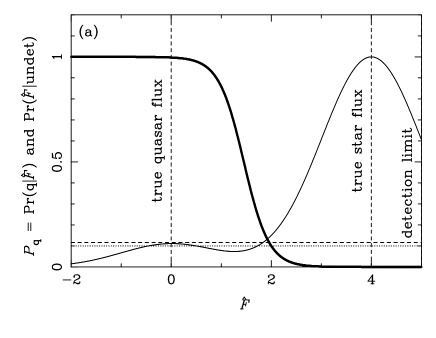
The fact that upper limits can be self-consistently included in the classification formalism does not, however, change the fact that they represent a loss of information. There are several ways in which this information loss could be characterised, but the most relevant here is how ${\rm{Pr}}({t}|\mbox{\boldmath${d}$},{\mathrm{det}})$ is changed. Given that the signal–to–noise ratio of a non-detection is inevitably low, it might seem that the effect of replacing a noisy flux estimate with an upper limit would be minimal. In the case of the HZQ candidates considered in Section 3, however, a ‘non-detection’ of, e.g., $\hat{F}_{b}\simeq 3\sigma_{b}$ is often sufficient to decisively reject a candidate. A simple example demonstrating why this is the case is presented in Appendix A.

While it is useful to be able to include upper limits, flux estimates should be supplied and used if possible. In particular, flux estimates are obtained for all non-detections in the UKIDSS–SDSS quasar search described in Section 3 and hence the calculations of $P_{\mathrm{q}}$ presented in Section 3.6 are based exclusively on Eq. (6), not Eq. (7).

2.2 The probability that a source is a HZQ

The probabilistic classification formalism described above was developed specifically to assess the quality of the numerous superficially promising quasar candidates that are inevitably generated by a HZQ survey. For a real point–source in such a sample only two possibilities are explicitly considered here: it is a Galactic star (i.e. ${t}={\mathrm{s}}$); or it is a target HZQ (i.e. ${t}={\mathrm{q}}$). Thus the model space is reduced to $\mbox{\boldmath${{t}}$}=\{{\mathrm{q}},{\mathrm{s}}\}$ and Eq. (4) can be simplified to give the quasar probability as

$$P_{\mathrm{q}}={\rm{Pr}}({\mathrm{q}}|\mbox{\boldmath${d}$},{\mathrm{det}})=\frac{W_{\mathrm{q}}(\mbox{\boldmath${d}$},{\mathrm{det}})}{W_{\mathrm{q}}(\mbox{\boldmath${d}$},{\mathrm{det}})+W_{\mathrm{s}}(\mbox{\boldmath${d}$},{\mathrm{det}})}.$$ (8)

The notation used in Eq. (8) emphasizes the role of the data in calculating $P_{\mathrm{q}}$, in the case of HZQs, but the most important single factor is the degree to which quasars are out-numbered by Galactic stars (at the depths probed by current surveys, at least). For this reason, $P_{\mathrm{q}}\ll 1$ unless a source not only has the measured colours of a HZQ, but has sufficiently precise photometry that the data represent a statistically significant deviation from the stellar locus. An implication of these criteria is that it is almost impossible for faint sources close to a survey’s detection limit to have high $P_{\mathrm{q}}$ as their measured colours are inevitably imprecise – almost all such sources with HZQ-like colours are better explained as being scattered stars. In the space of possible multi-band measurements and errors there is at best only a small region for which the quasar probability is significant – if the survey is too shallow or does not cover the appropriate wavelengths then $P_{\mathrm{q}}$ will be low for all possible photometric measurements. The Bayesian approach to candidate selection is, in principle, as exacting as possible; the next step is to see how it works in practice by applying it to a real data-set.

3 Searching for HZQs using UKIDSS and SDSS data

The probabilistic approach to HZQ selection described in Section 2 was developed to prioritse the large number of candidates generated by matching NIR UKIDSS sources to optical SDSS catalogues. The generation of the cross-matched UKIDSS–SDSS sample and the initial candidate selection are described in Section 3.1. Realistic models for the star and quasar populations are developed in Section 3.2 and Section 3.3, respectively. The dependence of the quasar probability, $P_{\mathrm{q}}$, on the measured photometry of an idealised source is explored in Section 3.4, and the possibilities for photometric redshift estimation are demontrated in Section 3.5. Finally, the probabilistic selection method is applied to the full UKIDSS–SDSS sample in Section 3.6.

3.1 Initial candidate selection

The starting point for this search for $z\ga 6$ quasars is UKIDSS (Lawrence et al., 2007), a suite of five separate NIR surveys using the Wide Field Camera (WFCAM; Casali et al. 2007) on the United Kingdom Infrared Telescope (UKIRT). A detailed technical description of the survey is given by Dye et al. (2006), although there have been a number of improvements in the time since (Warren et al., 2007). The most relevant of the projects is the Large Area Survey (LAS), which should eventually cover $\sim\!3800{\mbox{\rm\,\,\mbox{${\mathrm{deg}}^{2}$}}}$ in the UKIDSS $Y$, $J$, $H$ and $K$ bands (defined in Hewett et al. 2006). As of UKIDSS’s Seventh Data Release (DR7), on 2010 February 25, the LAS had covered $\sim\!1900{\mbox{\rm\,\,\mbox{${\mathrm{deg}}^{2}$}}}$ in $Y$ and $J$ to average depths of $\mbox{$Y$}_{\mathrm{lim}}=20.0\pm 0.1$ and $\mbox{$J$}_{\mathrm{lim}}=19.5\pm 0.2$ (Dye et al., 2006; Warren et al., 2007). Querying the WFCAM Science Archive (WSA; Hambly et al. 2008) reveals that the DR7 LAS sample contains $\sim\!2.2\times 10^{7}$ catalogued sources that were detected in both $Y$ and $J$. According to the QLF of Jiang et al. (2008), only $\sim\!10$ HZQs are expected with $\mbox{$Y$}\leq 19.8$ in the DR7 LAS area; the problem, then, is to identify these few sources efficiently and reliably.

The first step in the filtering process is to match the NIR UKIDSS sample to the optical catalogues from the SDSS (York et al., 2000). As of Data Release 7 (DR7; Abazajian et al. 2009), the SDSS covers $\sim\!1.2\times 10^{4}{\mbox{\rm\,\,\mbox{${\mathrm{deg}}^{2}$}}}$, including almost the entire UKIDSS LAS area. Observations were made in the custom $u$, $g$, $r$, $i$ and $z$ filters (Fukugita et al., 1996), and photometry was obtained in all five bands for every detected source. For point–sources the photometry was based on a model of the point-spread function (PSF). The SDSS main survey reaches single-scan depths of $\mbox{$i$}_{\mathrm{lim}}\simeq 22.5\pm 0.2$ and $\mbox{$z$}_{\mathrm{lim}}\simeq 20.8\pm 0.2$, and so sources close to the UKIDSS $Y$-band limit with $\mbox{$\mbox{$i$}$$-$$Y$}\ga 2.5$ and $\mbox{$\mbox{$z$}$$-$$Y$}\ga 0.8$ are likely to be undetected by SDSS. In the case of non-detections, aperture photometry in the $i$ and $z$ bands was obtained from the SDSS images. Aperture photometry was not obtained in the three bluest SDSS bands, however, although potential quasar candidates were rejected if they were detected in $u$, $g$ or $r$. More importantly, approximately $30\,{\mathrm{per\ cent}}$ of UKIDSS sources were observed more than once by SDSS, and in such cases the best flux estimates from the different scans (i.e. PSF-based if available or aperture otherwise) were combined using inverse-variance weighting. The final result is a combined UKIDSS–SDSS catalogue of sources with the best available survey photometry in the $i$, $z$, $Y$ and $J$ bands (as well as $H$ and $K$, where available).

Figure 1: Two-colour diagram showing the $\sim\!1.1\times 10^{4}$ UKIDSS DR7 LAS point–sources which, after being cross-matched to SDSS, have measured colours similar to those expected of HZQs. Also shown are the colours of the stellar locus described in Section 3.2 and the twelve quasars models described in Section 3.3, all calculated for a source that has $Y=19.5$. The dashed lines denote the initial pre-selection cuts that are applied before subsequent processing. The horizontal dotted line shows the maximum $i$$-$$Y$ value that a $Y=19.5$ source could have in the absence of noise.

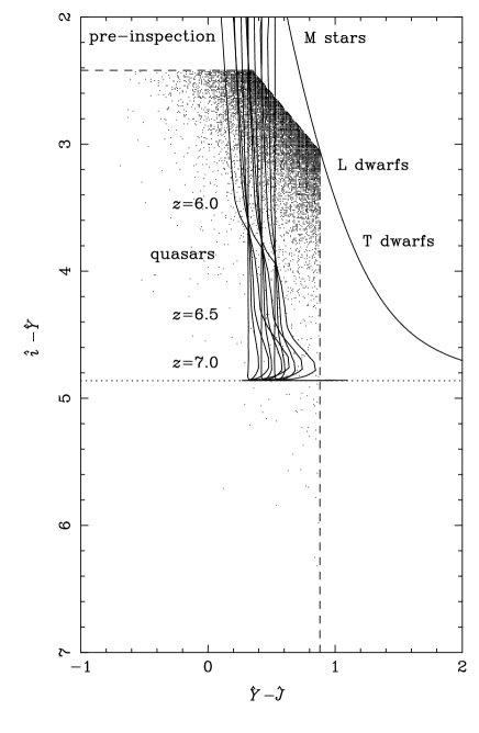
In the absence of photometric noise, the target HZQs are expected to occupy a region of the $i$, $z$, $Y$ and $J$ UKIDSS–SDSS colour space that is well separated from other astronomical sources (cf. Hewett et al. 2006). The theoretical separation between HZQs and cool stars in colour space is illustrated in Fig. 1, which shows both the stellar locus (described in Section 3.2) and the model quasar tracks (described in Section 3.3). The single dominant factor that ensures HZQs have such distinct colours is the near-complete absorption blueward of the Ly $\alpha$ emission line due to intervening H i. In the redshift range $5.8\la z\la 6.4$ Ly $\alpha$ is in the $z$ band, and so such quasars should be extremely red in $i$$-$$z$ (and $i$$-$$Y$); at higher redshifts ($6.6\la z\la 7.2$), Ly $\alpha$ is in the $Y$ band, leading to extremely red $z$$-$$Y$ or $i$$-$$Y$ colours. By contrast, most Main Sequence stars are expected to have considerably bluer colours, although the coolest M dwarfs have $\mbox{$\mbox{$i$}$$-$$Y$}\simeq 2$. While L and T dwarfs have similar $i$$-$$Y$ colours to HZQs, they are expected to be significantly redder in $Y$$\!\,-$$J$ (Hewett et al., 2006), which is the reason that the HZQ search only includes fields with observations in both $Y$ and $J$.

The vast majority of UKIDSS–SDSS sources can be rejected as HZQ candidates using a variety of automated cuts (described more fully in Mortlock et al. 2011): sources with an unambigous, bright match in SDSS that gives $\mbox{$\hat{i}$$-$$\hat{Y}$}\la 3$ are far bluer than the target HZQs; sources with red optical–NIR colours but with $\mbox{$\hat{Y}$$\!\,-$$\hat{J}$}\ga 0.9$ are almost certainly brown dwarfs; most galaxies appear as extended sources in UKIDSS (as characterised by, e.g., the UKIDSS MergedClassStat statistic); sources close to a bright star, or that have required deblending in the SDSS processing, or with significant UKIDSS error flags, all have unreliable measured photometry; sources with a significantly non-zero measured proper motion cannot be extra-Galactic. Applying these cuts to the SDSS-matched UKIDSS DR7 LAS catalogue leaves $\sim\!10^{4}$ apparently stationary, isolated point–sources that have the measured colours of HZQs. This sample is shown in Fig. 1, along with with the inclusive colour cuts that were adopted.

How should the HZQ search proceed from here? The ideal would be to take spectra of all of the candidates, but doing so would require prohibitive observational resources – Glikman et al. (2008) needed 25 hour-long Keck observations to rule out the most promising candidates from just the $27.3{\mbox{\rm\,\,\mbox{${\mathrm{deg}}^{2}$}}}$ covered by the UKIDSS Early Data Release (EDR; Dye et al. 2006). Obtaining independent photometry of all the candidates is more feasible, but still difficult due to limitations of telescope scheduling and the range of target right ascensions. Even if the intention was to reobserve all candidates, some means of prioritizing the most promising is needed – it is clear from Fig. 1 that a randomly selected candidate from this sample will almost certainly be a scattered Galactic star. It was this dilemma that led to the development of the Bayesian selection method described in Section 2. Before it can be implemented, however, models are needed for both the star and quasar populations.

3.2 The stellar population

Figure 2: The best-fit intrinsic distribution of $i$$-$$Y$ colours, $\rho_{\star}(Y+\mbox{\mbox{$i$}$-$$Y$},Y)$ for different values of $Y$ as labelled.

The UKIDSS–SDSS sources described in Section 3.1 have the measured colours of HZQs, but are predominantly Galactic stars (as can be seen from Fig. 1). The detailed optical and NIR properties of the various possible contaminants are described in detail by Hewett et al. (2006), but it is critical here to establish likely make-up of the contaminating sources in detail. Most Main Sequence stars are sufficiently hot that optical and NIR filters (and $i$, $z$, $Y$ and $J$ in particular) only probe their Rayleigh–Jeans tails. With $\mbox{$\mbox{$i$}$$-$$Y$}\simeq 1$, such stars are so much bluer than the target HZQs that they are not a significant contaminant. Cooler M stars also have bluer optical-NIR colours than the target HZQs (e.g. $\mbox{$\mbox{$i$}$$-$$Y$}\simeq 2$ as compared to $\mbox{\mbox{$i$}$-$$Y$}\ga 3$ for the quasars), but can be sufficiently faint in the $i$ band that a small fraction scatter to have $\mbox{$\hat{i}$$-$$\hat{Y}$}\ga 3$. Moreover, M stars have $\mbox{$Y$$\!\,-$$J$}\simeq 0.5$, much like the HZQs, and so the fact that their $Y$ and $J$ band photometry is typically fairly accurate actually increases the chance that some have the same observed colours as HZQs in the UKIDSS and SDSS bands. Conversely, the accurate $Y$$\!\,-$$J$ values measured for L and T dwarfs (which can be just as red in optical–NIR colours as HZQs) combines with their lower numbers to ensure that they are not the major source of contamination. As even the faintest sources considered as possible HZQ candidates have signal–to–noise ratios of $\ga 10$ in the $Y$ and $J$ bands, the number of rare L or T dwarf with $\mbox{$Y$$\!\,-$$J$}\ga 1.0$ being measured to have $\mbox{$\hat{Y}$$\!\,-$$\hat{J}$}\simeq 0.4$ is considerably less than the number of more common M stars measured to have $\mbox{$\hat{i}$$-$$\hat{Y}$}\ga 3$. As candidate lists based on simple colour cuts are dominated by scattered cool M dwarfs (with some L and T dwarfs), an accurate model of the intrinsic distribution of M, L and T dwarfs in the UKIDSS–SDSS bands is necessary to calculate useful values of $P_{\mathrm{q}}$. In more visual terms, the only sources that need to be modelled are those shown in Fig. 1 and the above arguments (along with the follow-up observations described in Section 3.6) show that these are predominantly M dwarfs.

There are several possible approaches for modelling the stellar population. One option would be to fit the distribution of observed colours or magnitudes (cf. Richards et al. 2004; Bovy et al. 2010), although this would not not correctly recover the tails of the (magnitude-dependent) noise distributions which are critical to this problem. Under the approximation that most of the relevant sources are sufficiently faint to be dominated by background noise (cf. Section 2.1), it might be possible to combine deconvolution techniques to estimate the instrinsic distribution (cf. Bovy et al. 2010), but this approach was not explored here. The other extreme would be to develop a physical model for the local population of M, L and T dwarfs, although the gain from this extra complication is minimal: it is only important to describe the distribution of measurable properties of these sources.

An intermediate approach to modelling the source population was adopted here. The population of nearby M, L and T dwarfs was described by developing a parameterized function to describe their intrinsic (i.e. not noise-convolved) distribution of magnitudes and colours. The reason for modelling the intrinsic distribution is to be able to estimate the probability of stars scattering into sparsely populated regions of colour space. While the core of the observed stellar distribution could be modelled empirically using the distribution of observed colours, such an approach would not provide reliable estimates of the probability of a source being scattered into the tails of the distribution (where the plausible HZQ candidates lie). It is better to model separately the intrinsic population and the noise distribution (Section 2.1) and to then convolve the two to provide the desired extreme scattering probability.

The adopted stellar population model has two parameters, $i$ and $Y$, both of which are observables. In terms of the notation of Section 2, the parameter space is defined by $\mbox{\boldmath${\theta}$}_{\mathrm{s}}=\{\mbox{$i$},\mbox{$Y$}\}$ and the number density of stars per unit solid angle is thus written as $\rho_{\mathrm{s}}(\mbox{\boldmath${\theta}$}_{\mathrm{s}})=\rho_{\mathrm{s}}(\mbox{$i$},\mbox{$Y$})$. With $i$$-$$Y$ serving as a proxy for stellar temperature, the other colours (i.e. $z$$-$$Y$ and $Y$$\!\,-$$J$) are, to a sufficiently good approximation, functions of $i$$-$$Y$. The specific form of $\rho_{\mathrm{s}}(\mbox{$i$},\mbox{$Y$})$ was obtained by comparing the predicted distribution of observed photometry to a sample of well-measured UKIDSS–SDSS point–sources (with $15.0\leq\hat{Y}\leq 19.5$ and $\mbox{$\hat{i}$$-$$\hat{Y}$}\geq 2.0$) extracted from the WSA. It was critical to ensure that the distribution describing the intrinsic population was convolved with the correct photometric noise distribution when comparing with the observed counts; a full description of the fitting procedure is given in Appendix B.

Several different functional forms for $\rho_{\mathrm{s}}(\mbox{$i$},\mbox{$Y$})$ were investigated before adopting power-law number counts in combination with an exponential power-law colour distribution for the reddest stars. Taken together,

$$\rho_{\mathrm{s}}(\mbox{$i$},\mbox{$Y$})=\rho_{*}10^{\alpha(Y-18.0)}$$

$$\mbox{}\,\,\,\,\,\,\,\times\Theta(\mbox{\mbox{$i$}$-$$Y$}-2)\frac{[\ln(\beta+\gamma Y)]^{1/\delta}\,(\beta+\gamma Y)^{-(i\mbox{--}Y)^{\delta}}}{P\left[1/\delta,\ln(\beta+\gamma Y)\,2^{\beta+\gamma Y}\right]},$$ (9)

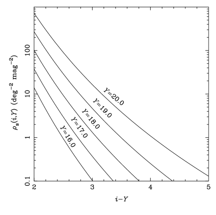
where $P(t,x)=\int_{x}^{\infty}{x^{\prime}}^{t-1}e^{-x^{\prime}}\,{\mathrm{d}}x^{\prime}$ is the complementary incomplete gamma function and the best-fit values of the free parameters are $\rho_{*}=20.9{\mbox{\rm\,\,mag}}^{-2}{\mbox{\rm\,\,deg}}^{-2}$, $\alpha=0.45939287$, $\beta=551.74630495$, $\gamma=-16.49969157$ and $\delta=0.04050890$. The best-fit distribution $\rho_{\mathrm{s}}(\mbox{$i$},Y)$ is shown as a function of $i$$-$$Y$ for several values of $Y$ in Fig. 2.

The model represents an average of the stellar population over the range of Galactic latitudes, $b$, covered by the UKIDSS LAS. The LAS was deliberately designed to avoid low-$b$ fields, so the stellar density of the reddest stars (which are seen only to moderate distances) varies by less than a factor of $\sim\!2$ over the whole survey area. Taking $W^{\prime}_{\mathrm{s}}(\mbox{\boldmath${d}$},{\mathrm{det}})\simeq 2W_{\mathrm{s}}(\mbox{\boldmath${d}$},{\mathrm{det}})$ in Eq. (8), would decrease $P_{\mathrm{q}}$ by a factor of $\sim\!5$ at most; and, for the vast majority of sources which are decisively classified, $P_{\mathrm{q}}$ remains essentially unchanged. In only a small fraction of cases would a poor candidate be erroneously included for follow-up due to this effect. For a survey covering a greater range of Galactic latitudes it would be important to include the $b$-dependence of $\rho_{\mathrm{s}}(\mbox{$i$},Y)$, most simply by multiplying $W_{\mathrm{s}}(\mbox{\boldmath${d}$},{\mathrm{det}})$ by a $b$-dependent scaling, the nature of which could be inferred from the survey data.

The predicted photometry in the other relevant bands (specifically $z$ and $J$) is then given by the empirical colour relations

$$\mbox{\mbox{$z$}$-$$Y$}=0.362+0.314\,(\mbox{\mbox{$i$}$-$$Y$})$$ (10)

and

$$\mbox{$Y$$\!\,-$$J$}=0.328+0.088\,(\mbox{\mbox{$i$}$-$$Y$})+0.0295\,(\mbox{\mbox{$i$}$-$$Y$})^{2}.$$ (11)

The two colour relationships in Eqs (10) and (11), together with the data, combine to give the likelihood (Eq. 5) as a function of $i$ and $Y$. Integrating the product of the likelihood and the stellar density (given in Eq. 9) over these two parameters then gives the weighted evidence that a source is a star, $W_{\mathrm{s}}(\mbox{\boldmath${d}$},{\mathrm{det}})$, as defined in Eq. (3). To be more explicit, specialising to the stellar case and the UKIDSS–SDSS filters allows Eq. (3) to be written as

$$W_{\mathrm{s}}(\hat{i},\hat{\mbox{$z$}},\hat{Y},\hat{z},{\mathrm{det}})$$ (12)

$$\mbox{}=\int_{-\infty}^{\infty}\int_{-\infty}^{\infty}\rho_{\star}(\mbox{$i$},Y)\,{\rm{Pr}}({\mathrm{det}}|\mbox{$i$},Y,{\mathrm{s}})\,{\rm{Pr}}(\hat{i},\hat{\mbox{$z$}},\hat{Y},\hat{z}|\mbox{$i$},Y,{\mathrm{s}})\,{\mathrm{d}}\mbox{$i$}\,{\mathrm{d}}Y.$$

The colour relationships in Eqs (10) and (11) combine with the $i$ and $Y$ to give the predicted photometry in the four bands of interest, from which the conversion to flux units allows the likelihood to be written as a product of four Gaussians (Section 2.1). The detection probability is close to unity for the range of $i$ and $Y$ being considered, although in practice adopting detection cut-offs is the simplest way to ensure the integrals do not extend to such faint fluxes that confusion issues would become relevant.

3.3 The quasar population at high redshift

UKIDSS is the first survey to have had a significant chance of detecting $z\simeq 7$ quasars, so there are no empirical constraints on much of the target HZQ population. This does not, however, mean that there is no information about the HZQ population beyond the current redshift limit – it is perfectly reasonable to extrapolate from the results of $z\simeq 6$ quasar surveys. Indeed, one of the main principles of Bayesian reasoning is that any available information should be applied if possible, even if it is incomplete or imprecise. A reasonable approximation to the correct prior (given by the actual, but unknown, QLF in this case) will result in final inferences that are superior to those derived from any method which does not include any information about the likely numbers of $z\simeq 7$ quasars. The alternative approach is, in the case of rare object searches, inevitably overly optimistic (i.e. $P_{\mathrm{q}}$ would be unreasonably high for large numbers of sources).

The measured numbers of bright HZQs (e.g. Fan et al. 2003; Jiang et al. 2008; Willott et al. 2010) are consistent with a co-moving QLF given by a power-law of the form

$$\Phi_{\mathrm{q}}(M,z)$$

$$\mbox{}=5.2\times 10^{-9}10^{0.84(M+26.0)-0.47(z-6.0)}{\mbox{\rm\,\,mag}}^{-1}{\mbox{\rm\,\,Mpc}}^{-3}.$$ (13)

This parameterisation combinines the magnitude dependence measured by Fan et al. (2003) with the evolution model used by Jiang et al. (2008). Willott et al. (2010) found a significantly lower normalisation than Jiang et al. (2008), and in principle the implied uncertainty should be included in the calculation of $P_{\mathrm{q}}$. However the resultant probabilities are unchanged in almost all cases, and the higher normalisation was adopted to ensure a (marginally) more inclusive candidate list. (Moreover, the above values were already being used to select UKDISS HZQ candidates before the results of Willott et al. 2010 were available.)

It would be possible to use $M$ and $z$ to parameterize the quasar population, but it is more intuitive to convert $M$ to the observable $Y$-band magnitude, so that the quasar population is, like the stellar population defined in Section 3.2, characterised by an observable surface density. Thus the quasar parameters used are $\mbox{\boldmath${\theta}$}_{t}=(Y,z)$, which leads to the population model

$$\rho_{\mathrm{q}}(Y,z)=\frac{1}{4\pi}\frac{{\mathrm{d}}V_{\mathrm{co}}}{{\mathrm{d}}z}\,\Phi_{\mathrm{q}}\left[Y-D_{\mathrm{L}}(z)-K_{Y}(z),z\right],$$ (14)

where ${\mathrm{d}}V_{\mathrm{co}}$ is the co-moving volume of a spherical shell of thickness ${\mathrm{d}}z$ at redshift $z$, $D_{\mathrm{L}}(z)$ is the luminosity distance and $K_{Y}(z)$ is the $Y$-band quasar $K$-correction that converts the rest-frame AB magnitude at $0.1450{\mbox{\rm\,\,\micron}}$ to the $Y$-band Vega magnitude.

The quasars’ $K$-corrections are, in turn, evaluated using updated and expanded versions of the model quasar spectra developed by Hewett et al. (2006) and Maddox et al. (2008). In particular, they include a realistic model of the absorption blueward of the Ly $\alpha$ emission line caused by the increased density of H i above $z\simeq 5.8$, as measured by Fan et al. (2006). The variety of the quasars’ intrinsic properties is accounted for by using colours from twelve different templates that span four line-strengths and three continuum slopes. As the main motivation of using multiple models is to ensure appropriately high values of $P_{\mathrm{q}}$ for the HZQs with redder continuum slopes (that are closer to the stellar locus in $Y$$\!\,-$$J$ than the fiducual quasars), the twelve models are weighted equally, even though it would be more accurate to down-weight the less common templates. Using a range of models also accounts for the colour variations that result from the combination of intrinsic quasar variability and non-simultaneous measurements: most UKIDSS observations took place several years after the SDSS observations of the same fields, a time-scale on which Ivezić et al. (2004) found a typical variation of $\sim\!0.15{\mbox{\rm\,\,mag}}$. When multiplied by the SDSS and UKIDSS filter profiles and integrated over wavelength, the model spectra not only give $K_{Y}(z)$, but also the required optical-NIR colours. All twelve colour tracks are shown in Fig. 1.

The HZQ colour relationships described above, together with the data, combine to give the likelihood (Eq. 5) as a function of $z$ and $Y$. Integrating the product of the likelihood the quasar density (given in Eq. 14) over these two parameters then gives the weighted evidence defined in Eq. (3) as

$$W_{\mathrm{q}}(\hat{i},\hat{\mbox{$z$}},\hat{Y},\hat{z},{\mathrm{det}})$$ (15)

$$=\int_{0}^{\infty}\!\!\int_{-\infty}^{\infty}\rho_{\mathrm{q}}(Y,z)\,{\rm{Pr}}({\mathrm{det}}|Y,z,{\mathrm{q}})\,{\rm{Pr}}(\hat{i},\hat{\mbox{$z$}},\hat{Y},\hat{z}|Y,z,{\mathrm{q}})\,{\mathrm{d}}Y\,{\mathrm{d}}z.$$

The quasar model loci give the predicted $i$, $z$, $Y$ and $J$ photometry, from which the conversion to flux units allows the likelihood to be written as a product of four Gaussians (Section 2.1). As with the integral over the stellar population (Eq. 12), a simple detection cut-off is needed to ensure that the integral is not dominated by the numerous undetectable ultra-faint sources that are beyond the confusion limit in the relevant bands.

3.4 The probability that a source is a HZQ

Having developed quantitative models for the stellar population (Section 3.2) and HZQ population (Section 3.3), the measured $i$, $z$, $Y$ and $J$ band photometry of a source can then be used to calculate $P_{\mathrm{q}}$ according to Eq. (4). The two-dimensional (weighted) evidence integrals over the quasar and star parameters are evaluated using simple numerical quadrature as this is faster than more general Monte Carlo techniques for a problem of such low dimensionality. On a standard desktop computer one evaluation of $P_{\mathrm{q}}$ takes between a tenth and a hundredth of a second, which is sufficiently fast that even the most inclusive of candidate lists can be analysed.

The speed with which $P_{\mathrm{q}}$ can be calculated also means that it is possible to explore how $P_{\mathrm{q}}$ depends on the measured photometry and the associated errors. This is potentially important, as the reasons that some candidates have low or high probabilities are not always obvious. In this context it is useful to think of $P_{\mathrm{q}}$ not as a quantity associated with candidates, but as a function of the information that is particular to each source (i.e. the measured photometry and the associated uncertainties), leading to $P_{\mathrm{q}}=P_{\mathrm{q}}(\hat{i},\Delta\hat{i},\hat{\mbox{$z$}},\Delta\hat{\mbox{$z$}},\hat{Y},\Delta\hat{Y},\hat{J},\Delta\hat{J})$ for the UKIDSS–SDSS sample. This function has too many parameters to explore comprehensively, but many of its important features can be seen in two-dimensional projections. Plotting $P_{\mathrm{q}}$ in the space of measured colours also facilitates direct comparison with selection methods based on colour cuts, which can be cast into a Bayesian form by treating them as if $P_{\mathrm{q}}=1$ for objects satisfying the cuts and $P_{\mathrm{q}}=0$ otherwise. In the regions of parameter space for which $P_{\mathrm{q}}$ varies rapidly with the measured colours, the Bayesian selection reduces to a cut-based method, but with the important difference that the selection boundaries are defined objectively.

Figure 3: The dependence of $P_{\mathrm{q}}$ on the measured $z$ band magnitude for different value of the measured $i$$-$$z$ colour, ranging from $P_{\mathrm{q}}=0$ (white) to $P_{\mathrm{q}}=1$ (grey). The noise is as appropriate for fiducial SDSS observations with $\mbox{$i$}_{{\mathrm{lim}}}=22.5$, $\mbox{$z$}_{{\mathrm{lim}}}=20.8$, but the UKIDSS bands ($Y$ and $J$) have been ignored. The dashed line shows the initial SDSS HZQ selection criterion defined in Fan et al. (2003) and the dotted line shows the maximum theoretical value of $i$$-$$z$ for a source with $\mbox{$z$}=\hat{\mbox{$z$}}$ and zero flux in the $i$ band in the absence of noise.

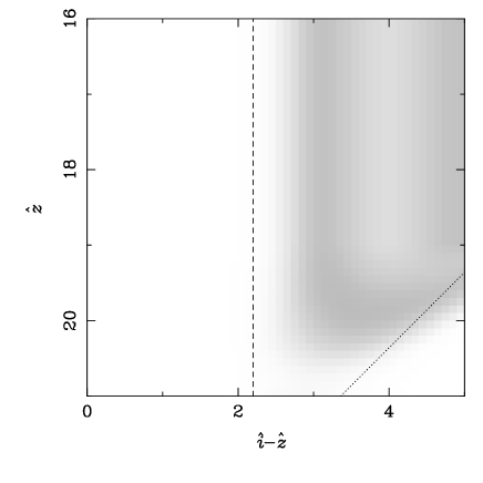
The simplest non-trivial case is that of a two-band survey for which each detected source can be treated as having one measured magnitude and a single measured colour. If the two bands are taken to be $i$ and $z$, this is a reasonable approximation to the SDSS HZQ survey, for which the initial selection criteria were $\hat{\mbox{$z$}}<20.2$ and $\mbox{$\hat{i}$$-$$\hat{\mbox{$z$}}$}>2.2$ (Fan et al., 2001). Ignoring the $Y$ and $J$ bands and assuming the fiducial SDSS depths in $i$ and $z$ given in Section 3.1, the variation of $P_{\mathrm{q}}$ with $\hat{\mbox{$z$}}$ and $\hat{i}$$-$$\hat{\mbox{$z$}}$ is shown in Fig. 3. The only sources which have $P_{\mathrm{q}}\ga 0.1$ are those which have $\hat{\mbox{$z$}}\la 20$ and $\hat{i}-\hat{\mbox{$z$}}\ga 2.5$, roughly corresponding to the region of parameter space selected by Fan et al. (2001). The seemingly counter-intuitive result that the $P_{\mathrm{q}}$ does not increase monotonically with $i$$-$$z$ is an artefact of the asinh magnitude system.

It is also noticeable from Fig. 3 that no pair of (measured) $\hat{i}$ and $\hat{\mbox{$z$}}$ values would result in $P_{\mathrm{q}}\simeq 1$, a result which is independent of the depth of the observations. This is because the sources which appear red in $i$$-$$z$ are not just scattered stars, but also L and T dwarfs which actually have these red colours (and outnumber the target HZQs). The only way to generate a sample of candidates with higher $P_{\mathrm{q}}$ is to obtain data in another band, chosen such that quasars and the potential contaminants have distinct colours. This can be done by follow-up (e.g. in the $J$ band, as done by Fan et al. 2001) or by extending the wavelength coverage of the inital survey (e.g. UKIDSS $Y$-band imaging). The choice between these two strategies is sometimes difficult, as adding an extra band to a survey costs area or depth, whereas the number of follow-up observations required to complete a two-band search is potentially prohibitive. However in terms of this exploration of how $P_{\mathrm{q}}$ depends on the measured colours there is no distinction, as only the observational depths and the choice of bands is important, not the sequence of observations.

Figure 4: The dependence of $P_{\mathrm{q}}$ on a source’s observed $i$$-$$z$ and $z$$-$$J$ colours, ranging from $P_{\mathrm{q}}=0$ (white) to $P_{\mathrm{q}}=1$ (grey), for $\hat{\mbox{$z$}}=18.5$, $\hat{\mbox{$z$}}=19.0$, $\hat{\mbox{$z$}}=19.5$ and $\hat{\mbox{$z$}}=20.0$, as labelled. In all cases the noise is as appropriate for fiducial SDSS and UKDISS observations with $\mbox{$i$}_{{\mathrm{lim}}}=22.5$, $\mbox{$z$}_{{\mathrm{lim}}}=20.8$ and $J_{{\mathrm{lim}}}=22.5$, but the $Y$ band has been ignored. The quasar and star loci are shown as solid curves and the dashed lines show the SDSS HZQ selection region defined in Fan et al. (2003).

Figure 5: The dependence of $P_{\mathrm{q}}$ on a source’s observed $i$$-$$Y$ and $Y$$\!\,-$$J$ colours, ranging from $P_{\mathrm{q}}=0$ (white) to $P_{\mathrm{q}}=1$ (grey), for $\hat{Y}=18.0$, $\hat{Y}=18.5$, $\hat{Y}=19.0$ and $\hat{Y}=19.5$, as labelled. In all cases the noise is as appropriate for fiducial SDSS and UKDISS observations with $\mbox{$i$}_{{\mathrm{lim}}}=22.5$, $Y_{{\mathrm{lim}}}=20.2$ and $J_{{\mathrm{lim}}}=22.5$, but the $z$ band has been ignored. The horizontal dotted line shows the maximum theoretical value of $i$$-$$Y$ for a source with $Y=\hat{Y}$ and zero flux in the $i$band in the absence of noise; this changes with $\hat{Y}$ due to the use of asinh magnitudes to represent the $i$ band photometry. The fiducial quasar and star loci are shown as solid curves and the dashed lines show the basic pre-selection made to generate the UKIDSS–SDSS candidate sample.

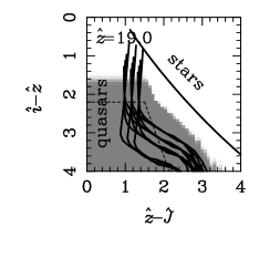
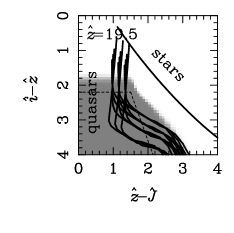
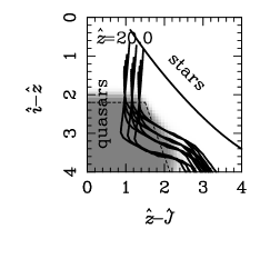
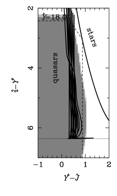
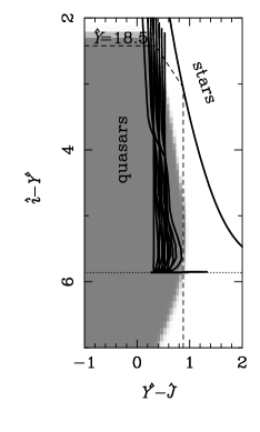
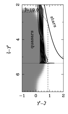
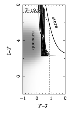
The above results imply that measurements in at least three bands are required to generate a sample of strong HZQ candidates, and in particular that two appropriately chosen colours are needed. Indeed, many HZQ searches have been based on pairs of colour cuts (e.g. Warren et al. 1994; Fan et al. 2001), and this approach is compared directly with the Bayesian results Figs. 4 and 5. In both cases the depths in the included bands are chosen to match the fiducual UKIDSS and SDSS values given in Section 3.1, but data in the missing band ($Y$ and $z$, respectively) is ignored. Figure 4 approximates the optical SDSS search of Fan et al. (2001) (but cannot mimic the CHFQS described by Willott et al. 2007 because the star and quasar models do not go sufficiently deep), whereas Fig. 5 represents one of the obvious selection options from the matched UKIDSS-SDSS data. As expected, $P_{\mathrm{q}}$ has a similar colour-dependence, being low near the stellar locus and higher where the quasars are expected to be found. There is also a strong correspondence between the region of high $P_{\mathrm{q}}$ and the specific selection region defined by Fan et al. (2003), particularly close to the the $z$-band selection cut at $\hat{\mbox{$z$}}=20.1$. There are, however, significant systematic differences between the Fan et al. (2003) selection region and the the high-$P_{\mathrm{q}}$ region. The most obvious difference is that $P_{\mathrm{q}}$ also varies with magnitude for a given set of measured colours. The most important aspect of the magnitude-dependence is the decrease in the size of the high-$P_{\mathrm{q}}$ region close to the detection limit in the reference band (i.e. as $\mbox{$z$}\rightarrow 20.8$ or $Y\rightarrow 20.2$). For sources well above the detection limit(s) the photometric errors are sufficiently small that there is only a minimal chance of such bright stars being measured with HZQ-like colours. But for fainter sources close to the detection limit the effective width of the observed stellar locus is greatly increased and, in the example shown in Fig. 4, encompasses the HZQ locus.

Figure 6: The dependence of $P_{\mathrm{q}}$ on a source’s observed $Y$-band magnitude given it has the observed $i$$-$$Y$, $z$$-$$Y$ and $Y$$\!\,-$$J$ colours of a HZQ with a redshift of $z=6.0$, $z=6.5$ and $z=7.0$, as labelled. The dashed horizontal line shows the cut of $P_{\mathrm{q}}=0.1$ used in selecting UKIDSS–SDSS candidates for follow-up and hence gives the approximate completeness limit of the HZQ survey at different redshifts.

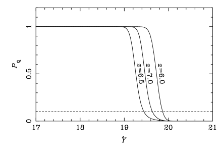
The somewhat counter-intuitive consequence is that a sample of sources with (nearly) identical measured colours can include both near-certain HZQs and obviously uninteresting scattered stars. The dependence of $P_{\mathrm{q}}$ on reference magnitude is shown in Fig. 6 for sources with the measured colours of quasars with redshifts of $z=6.0$, $z=6.5$ and $z=7.0$. HZQs over the whole redshift range of interest have $P_{\mathrm{q}}\simeq 1$ for $\hat{Y}\la 19$, after which $P_{\mathrm{q}}$ falls fairly sharply due to the greater numbers of stars scattered to have quasar-like colours. For each of the three redshift values the source’s measured colours are constant across the plot, and so it remains perfectly consistent with being a HZQ; the change comes about as the observed stellar locus is broader for higher $\hat{Y}$, and for $\hat{Y}\ga 19.5$ effectively covers the quasar loci. The redshift-dependence of the effective depth comes about due to the small variations of the HZQs’ $Y$$\!\,-$$J$ colour as various emission lines appear in different filters. As can be seen in Fig. 1, the expected $Y$$\!\,-$$J$ colours of HZQs increases from $\mbox{$Y$$\!\,-$$J$}\simeq 0.4$ at a redshift of $z\simeq 6.0$ to $\sim 0.6$ at a redshift of $z\simeq 6.8$, bringing them closer to the stellar locus. As a result the maximum depth at which they remain well-separated from the observationally-broadened stellar locus is decreased and the effective depth (defined as the $Y$ magnitude at which $P_{\mathrm{q}}=0.5$) decreases from $\hat{Y}\simeq 19.7$ at a redshift of $z\simeq 6.0$ to $\hat{Y}\simeq 19.3$ at a redshift of $z=6.5$. At higher redshifts, however, the small increase in $Y$$\!\,-$$J$ is much less important than the large increase in the HZQs’ expected $i$$-$$Y$ values. As a result the effective depth at a redshift of $z\simeq 7.0$ has increased to $\hat{Y}\simeq 19.5$. One implication of these various subtle effects is that the selection function of the UKIDSS–SDSS HZQ search given in Mortlock et al. (2011) is more strongly redshift-dependent than the SDSS (Fan et al., 2003) or CFHQS (Willott et al., 2010) selection functions.

Thus far the emphasis has been on the variation of $P_{\mathrm{q}}$ with the properties of a source, but it is also revealing to investigate how $P_{\mathrm{q}}$ depends on survey depth. Figure 7 shows how $P_{\mathrm{q}}$ varies with $i$ band depth (assuming a fiducial magnitude of $\hat{Y}=19.5$). As expected, extra depth in the $i$ band increases the confidence with which $z\simeq 6$ quasars can be identified. It is possible to push closer to the stellar locus (i.e. redder in $Y$$\!\,-$$J$) with confidence, and also possible to find fainter HZQs (i.e. going deeper in $Y$). Increasing the depth in the $Y$ or $J$ bands is not nearly as useful, because the $Y$$\!\,-$$J$ colour is already sufficiently well measured for a $\hat{Y}\simeq 19$ source. However extra depth in all three bands would allow a deeper survey, and hence greater numbers of HZQs, albeit of lower intrinsic luminosity. This variation also shows the importance of calculating $P_{\mathrm{q}}$ using the measured noise levels in each field of a survey, rather than just using generic survey-wide depths.

Figure 7: The dependence of $P_{\mathrm{q}}$ on a source’s observed $i$$-$$Y$ and $Y$$\!\,-$$J$ colours, ranging from $P_{\mathrm{q}}=0$ (white) to $P_{\mathrm{q}}=1$ (grey), for $\mbox{$i$}_{\mathrm{lim}}=21.5$, $\mbox{$i$}_{\mathrm{lim}}=22.5$, $\mbox{$i$}_{\mathrm{lim}}=23.5$ and $\mbox{$i$}_{\mathrm{lim}}=24.5$, as labelled. In all cases the noise is as appropriate for fiducial SDSS and UKDISS observations with $\mbox{$i$}_{{\mathrm{lim}}}=22.5$ and $J_{{\mathrm{lim}}}=22.5$, but the $z$ band has been ignored. The source has a measured $Y$ band magnitude of $\hat{Y}=19.5$ and measured $i$ and $J$ band magnitudes as implied by the observed colours. The horizontal dotted line shows the maximum theoretical value of $i$$-$$Y$ for a source with $Y=\hat{Y}$ and zero flux in the $i$band in the absence of noise; this changes with $\hat{Y}$ due to the use of asinh magnitudes to represent the $i$ band photometry. The quasar and star loci are shown as solid curves and the dashed lines show the basic pre-selection made to generate the UKIDSS–SDSS candidate sample.

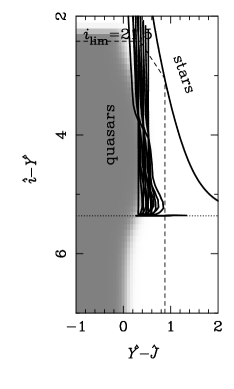
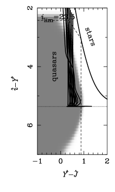
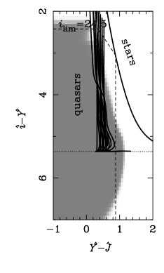
In almost all the above examples the transitions between regions of high and low $P_{\mathrm{q}}$ are quite sharp, with no large areas of uncertainty. The transition scale is set by the photometric errors, although for a given observation and reference magnitude (as is the case here) the errors vary with colour. This also explains why the transition is more gradual in regions of colour space which are expanded by the decreased variation of colour with flux, which is the case for red $\hat{i}$$-$$\hat{\mbox{$z$}}$ or $\hat{i}$$-$$\hat{Y}$ here. The one case of an obviously gradual transition is shown the right panel of Fig. 4, in which the source is sufficiently faint that the measurement uncertainties in all the relevant bands are $\ga 0.2{\mbox{\rm\,\,mag}}$.

3.5 Photometric redshift estimation

Figure 8: Posterior distributions of the redshifts of the seven HZQs in UKIDSS DR7 inferred from the UKIDSS–SDSS survey photometry. The eighth panel shows the results from a simulated $z=7$ quasar with $\hat{i}=24.35\pm 0.50$, $\hat{z}=22.10\pm 0.20$, $\hat{Y}=19.50\pm 0.020$ and $\hat{J}=19.06\pm 0.030$. Results for both a realistc (solid curve) and uniform (dashed curve) prior in the quasar’s redshift, $z$, and $Y$-band magnitude are shown. The vertical lines show the spectroscopic redshift in the case of the seven real sources and the simulated redshift in the case of the synthetic $z=7$ quasar.

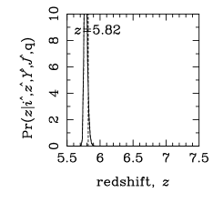
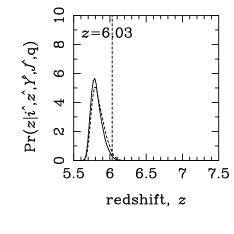
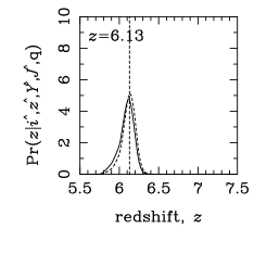
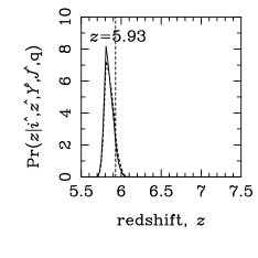
The most important information that can be extracted from the measurements of a candidate is the probability that it is a HZQ; but if the source is assumed to be a quasar then the photometry can also be used to estimate its likely redshift. Given that a spectrum is necessary to confirm any candidate as a quasar, there is little long-term utility of such photometric redshift estimates but they can useful in prioritizing follow-up observations of HZQ candidates. The essenetial logic that it is most efficient to pursue high-$P_{\mathrm{q}}$ objects first is somewhat modified by the fact that there is a particular premium on finding the most distant sources (i.e. HZQs with $z\ga 6.5$ in the case of UKIDSS). It would probably make more sense to follow-up a $z$-band drop-out $z\ga 6.5$ quasar candidate with $P_{\mathrm{q}}\simeq 0.1$ than a more secure candidate with $P_{\mathrm{q}}\simeq 0.9$ that was well-detected in the $z$ band (a fact which might have contributed to the high $P_{\mathrm{q}}$ in the first place).

The calculation is analagous to that used in Bayesian photometric redshift estimation of galaxies (e.g. Benítez 2000) but with the important difference that quasar spectra exhibit far less variety than those of galaxies, so that it is far easier to obtain reliable estimates. The posterior distribution of a (putative) quasar’s redshift, given photometric measurements $\hat{i}$, $\hat{\mbox{$z$}}$, $\hat{Y}$ and $\hat{J}$, is calculated by modifying Eq. (15) to marginalise only over the unknown true $Y$-band magnitude. That gives

$${\rm{Pr}}(z|\hat{i},\hat{\mbox{$z$}},\hat{Y},\hat{z},{\mathrm{q}},{\mathrm{det}})$$

$$\mbox{}=\frac{\int_{-\infty}^{\infty}\rho_{\mathrm{q}}(Y,z)\,{\rm{Pr}}({\mathrm{det}}|Y,z,{\mathrm{q}})\,{\rm{Pr}}(\hat{i},\hat{\mbox{$z$}},\hat{Y},\hat{z}|Y,z,{\mathrm{q}})\,{\mathrm{d}}Y}{W_{\mathrm{q}}(\hat{i},\hat{\mbox{$z$}},\hat{Y},\hat{z})},$$ (16)

where $\rho_{\mathrm{q}}(Y,z)$ is given in Eq. (14), the appropriate form of the likelihood, ${\rm{Pr}}(\hat{i},\hat{\mbox{$z$}},\hat{Y},\hat{z}|Y,z,{\mathrm{q}})$, is discussed in Section 2.1 and the denominator $W_{\mathrm{q}}(\hat{i},\hat{\mbox{$z$}},\hat{Y},\hat{z})$ ensures the probability is correctly normalised. (The posterior distribution in any of the model parameters – for either quasars or stars – could similarly evaluated by modifying Eq. 3 to marginalise over nuisance variables.)

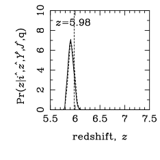
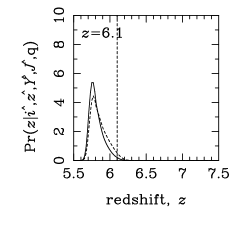
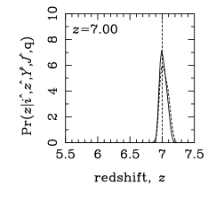
The results of evaluating Eq. (16) for the seven HZQs discovered in UKIDSS are shown in Fig. 8. In each case the posterior distributions inferred from the UKIDSS–SDSS survey photometry (under both realistic and fiducial uniform priors in $z$ and $Y$) are compared to the spectroscopically-measured redshift. The similarity of the distributions for the two different priors indicate that the detailed knowledge of the HZQ population is not important: the UKIDSS–SDSS photometric data (in combination with the model of the quasars’ colours) are sufficient to give largely prior-independent redshift estimates that have uncerainties of $\Delta z\simeq 0.1$. Moreover, these inferences are broadly verified by the subsequent spectroscopic redshift measurements, although there is a suggestion that the photometric estimates are systematically low. The basic success of this method is unsurprising – from Fig. 1 it is clear that a good measurement even of just $i$$-$$Y$ would be sufficient to obtain a reasonable redshift estimate – although the full precision depends on all the available photometry.

In the absence of any discoveries of HZQs with redshifts of $\ga 6.5$ in UKIDSS DR7, the photometric redshifts constraints obtained for a simulated $z=7.0$ quasar are shown the bottom-right panel of Fig. 8. Assuming that the extrapolation of the spectroscopic HZQ models described in Section 3.3 are valid, the photometric redshift constraints from UKIDSS–SDSS data are accurate to $\Delta z\simeq 0.1$ over the entire range $5.8\la z\la 7.2$. Any $z\ga 6.5$ candidates should thus be readily identifiable from the survey photometry and can prioritsed in the follow-up process.

3.6 Results

Figure 9: Histogram of the quasar probabilities, $P_{\mathrm{q}}$, of the most promising stationary point–sources in UKIDSS DR7. The dotted line shows all sources that passed the automatic filtering described in Section 3.1. The solid line shows the results after follow-up photometry. All the sources with $P_{\mathrm{q}}\geq 0.1$ have been inspected visually, whereas only a random fraction of sources with $P_{\mathrm{q}}<0.1$ have been inspected (in the earlier stages of the project, before the selection criteria were finalised), and so still include many contaminants. There are a small number of candidates with $0.1\leq P_{\mathrm{q}}\la 0.3$ that are yet to be reobserved.

Figure 10: Two-colour diagrams showing the UKIDSS DR7 LAS point–sources which, after being cross-matched to SDSS, have $P_{\mathrm{q}}\geq 0.1$ from the UKIDSS–SDSS survey photometry. The colours and from the survey photometry are shown in the left panel; the results of follow-up photometry are shown in the right panel (in which the open symbols are rejected candidates and the solid symbols are the seven confirmed HZQs in the UKIDSS DR7 sample). A single follow-up measurement (generally in the $i$ band) was sufficient to reject most candidates, so the some colours (most often $Y$$\!\,-$$J$) in the two panels remain the same; also, there are a few candidates which are yet to be reobserved and so appear at the same position in both panels (as do the previously known HZQs). Also shown are the colours of the twelve quasar models described in Section 3.3 and the stellar locus described in Section 3.2, in both cases calculated for a source that has $Y=19.5$. The dashed lines denote the initial pre-selection cuts that are applied before subsequent processing and the horizontal dotted line shows the maximum $i$$-$$Y$ value that a $Y=19.5$ source could have in the absence of noise.

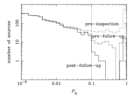
Having understood how the photometric measurements of a source combine with models of the star and quasar populations to give $P_{\mathrm{q}}$ (Section 3.4), the Bayesian selection method could be applied with confidence to the UKIDSS–SDSS sample of $\sim\!10^{4}$ candidate HZQs described in Section 3.1. The value of $P_{\mathrm{q}}$ was calculated for each source, and the high-probability tail of the resultant distribution is shown as the dotted histogram in Fig. 9. The main result was that the vast majority of sources with HZQ-like colours had $P_{\mathrm{q}}\ll 1$ and were not considered further. Given the low number of HZQs expected in the sample, the rejection of most candidates was both desireable and predictable, and immediately rendered the follow-up task far more manageable.

Applying a cut of $P_{\mathrm{q}}\geq 0.1$ left just 893 promising candidates in UKIDSS DR7, a completely automated reduction by a factor of $\sim\!2.5\times 10^{4}$ from the initial UKIDSS–SDSS sample. Having extracted essentially all the useful information from the photometry, the next step was to inspect the SDSS and UKIDSS images of the remaining candidates. Most of the candidates were, unsurprisingly, revealed to be spurious, with a large variety of explanations (see Mortlock et al. 2011 for more details): faint galaxies with supernovae that were present in the UKIDSS observations but absent when the SDSS observations were made; Solar System asteroids that were observed by UKIDSS close to turn-around; UKIDSS cross–talk or persistence (Dye et al., 2006); and various data artefacts that resulted in obviously incorrect photometry. In theory, all such contaminants could be included as additional models (along with stars and quasars) in the Bayesian classification scheme; but, aside from the difficulties in specifying the likely numbers and properties of these various contaminants, these contaminants are sufficiently rare that their identifcation does not consume significant resources.

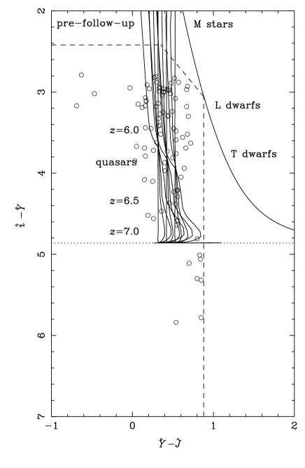
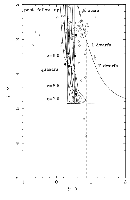
Of the 893 UKIDSS DR7 objects with $P_{\mathrm{q}}\geq 0.1$, only 88 were confirmed as real, stationary, astronomical sources with no obvious data problems that might result in erroneous photometry. Figure 10 shows the colours of these candidates both from the intial UKIDSS–SDSS survey photometry (left panel) and then updated after follow-up observations (right panel). The distribution of these (real) candidates’ quasar probabilities is shown as the dashed histogram in Fig. 9. The distribution of $P_{\mathrm{q}}$ values can be used as a guide to calibrate the probability calculation: if the models of the measurement process and the two populations were completely accurate then the sum of $P_{\mathrm{q}}$ over all the candidates would be approximately equal to the expected number of HZQs in the sample. That is not the case here: whereas only $\sim\!10$ HZQs are expected, the initial probability sum is $\sim\!60$ and the sum after follow-up observations is $\sim\!40$. The most plausible reason for these discrepancies is the use of a Gaussian likelihood (see Section 2.1) rather than a distribution with heavier tails to account better for outliers. The fact that the sum even after follow-up is still so high indicates that the probabilities even for poor candidates with $P_{\mathrm{q}}\la 0.01$ are systematically high. It is, however, the realtive probabilities (i.e. their rankings) that of primary importance – the real reason for exploring a Bayesian selection algorithm in the first place was not so much to determine the probability that the candidates are HZQs, but to answer the distinct question of which of the identified candidates were the most likely to be quasars.

Having ranked the candidates, the first stage of the follow-up campaign was to see whether any of the red UKIDSS–SDSS sources had been catalogued previously. Cross-matching with SDSS revealed that three of the highest-ranked objects were known HZQs (SDSS J083643.9$+$005453.2 at redshift $z=5.82$, Fan et al. 2001; SDSS J141111.3$+$121737.3 at redshift $z=5.93$, Fan et al. 2004; and SDSS J162331.8$+$311200.5 at redshift $z=6.22$, Fan et al. 2004). All three were very strong candidates with $P_{\mathrm{q}}\geq 0.99$ and so clearly would have been discovered by subsequent observations had they been required. The remaining candidates were all queued for follow-up photometric observations at The Liverpool Telescope ($i$ filter), The Isaac Newton Telscope ($i$ and $z$ filters) or UKIRT ($Y$ and $J$ filters). The follow-up images were generally deeper than the SDSS and UKIDSS survey observations, but even more important than an increase in photometric precision was that these new measurements were independent of the candidate selection process. Whereas the initial selection could be thought of as a method of identifying stars for which the SDSS measurements are faint in $i$ or in which the UKIDSS data are bright in $Y$, the follow-up photometry should be unbiased. Every time a measurement was made the quasar probability was recalculated with the new photometry; a candidate was discarded if $P_{\mathrm{q}}\la 0.01$ at any stage. Many candidates were rejected after just one follow-up observation, in most cases because they were revealed to be significantly brighter in the $i$ band than indicated by the initial survey photometry. These candidates can be seen with $\mbox{$\hat{i}$$-$$\hat{Y}$}\simeq 2.5$ in Fig. 10; as expected, their observed colours are much more like those of the reddest M dwarfs. (Further follow-up observations in the $Y$ band would probably reveal that the true $i$$-$$Y$ values are bluer still – as the initial sample was selected to be red in $i$$-$$Y$, the initial $Y$-band photometry of the candidates tends to be biased bright, just as their initial $i$-band photometry is biased faint.) It is also striking that a number of the rejected candidates still have the observed $i$$-$$Y$ and $Y$$\!\,-$$J$ colours of HZQs, again illustrating the strong role that the Bayesian priors (particularly the relative numbers of stars and quasars) play in this process.

If a candidate still had $P_{\mathrm{q}}\simeq 1$ after reobservation in at least the $i$, $Y$ and $J$ bands then spectroscopic observations were obtained. As detailed in Mortlock et al. (2011), spectra were taken of seven UKIDSS DR7 candidates: four were confirmed as new HZQs (Mortlock et al. 2009; Venemans et al. 2011; Patel et al. 2011). At the end of this follow-up process every source with $P_{\mathrm{q}}\geq 0.1$ from the UKIDSS–SDSS survey photometry should either be convincingly rejected or spectroscopically confirmed as a HZQ. This separation into sources with $P_{\mathrm{q}}\simeq 0$ and confirmed HZQs with $P_{\mathrm{q}}=1$ is a natural result of obtaining more information about those candidates that were initially promising but fundamentally ambiguous. The separation is not readily apparent in Fig. 10 as neither the $z$-band photometry nor the photometric errors are shown (and because a few candidates are yet to be followed up and so not yet decisively classified), but it is well illustrated by the solid histogram in Fig. 9.

The choice of a rigorous probability cut-off (i.e. $P_{\mathrm{q}}\geq 0.1$ here) is not necessary to maximize the yield from the survey in terms of HZQs numbers but is needed to evaluate the selection function (i.e. completeness) of the final sample. Indeed, the primary selection criterion for a HZQ of given intrinsic properties is that it has $P_{\mathrm{q}}\geq 0.1$ in the UKIDSS–SDSS survey photometry. The selection probability is not, however, equal to $P_{\mathrm{q}}$; rather it given by the fraction of HZQs that, when observed with the appropriate noise levels in the UKIDSS–SDSS bands, would have $P_{\mathrm{q}}\geq 0.1$. The selection probability is evaluated in Mortlock et al. (2011) as part of the estimation of the HZQ luminosity function from the UKIDSS DR7 data.

4 Conclusions

A probabilistic approach to quasar selection can, at least in principle, make use of all the relevant information about a candidate HZQ: knowledge of the quasar and star populations; the stochastic nature of the measurement process; and, of course, the data obtained for the source in question. Having derived a general Bayesian formalism for HZQ selection, this approach was applied to real quasar candidates taken from the cross-matched UKIDSS and SDSS data-sets. The $\sim\!1900{\mbox{\rm\,\,\mbox{${\mathrm{deg}}^{2}$}}}$ surveyed as of UKIDSS DR7 contained only 88 real astronomical sources with quasar probabilities of $P_{\mathrm{q}}\geq 0.1$, and most of these candidates were quickly rejected with follow-up photometry (a single $i$-band image sufficing in many cases). Aside from three known HZQs, this follow-up process left just seven strong photometric candidates, of which four were redshift $z\simeq 6$ quasars. If a cut-based approach had been adopted then follow-up observations would have been required for $\sim\!10^{3}$ candidates. Not only was the Bayesian selection method very efficient, but it was also entirely quantitive and objective, as needed to estimate the high-redshift QLF from the sample (see Mortlock et al. 2011).

It is also possible to combine this model-selection approach with parameter estimation. In the context of HZQs it is clear that the highest redshift objects are the most important, in which case $P_{\mathrm{q}}$ could be combined with an estimate of the putative quasar’s redshift to rank potentialy record-breaking HZQs above those at redshifts which have already been explored. Comparing the resultant photometric HZQ redshift estimates of the seven confirmed quasars with their spectroscopic redshifts confirms that the photometry is sufficiently imformative about a quasar’s redshift that it can be used to prioritize candidates in the follow-up process.

The Bayesian HZQ selection method described here will continue to be used in the analysis of subsequent UKIDSS data releases, and may also be applied to data from future NIR surveys such as Pan–STARRS (Kaiser et al., 2002) and VISTA (Emerson et al., 2004). The utility of – and need for – such a complicated approach to HZQ selection depends on the survey details: the bands used and the depths reached determine the degree to which the target HZQs are separated in colour space from the contaminating stellar population(s). In almost all cases, however, the applications of these Bayesian selection methods would represent a step closer to extracting as much science as possible from the available data by investigating fainter sources.

A corollary of the survey-dependent nature of Bayesian quasar selection is that the expected distribution of candidate probabilities could be a useful tool in survey design. This was particular apparent by the degree to which the high-$P_{\mathrm{q}}$ region of the SDSS data space matched the HZQ colour cuts adopted by Fan et al. (2001). Given that the trade-off between broader filters (giving a higher signal–to–noise ratio) and narrower filters (giving better-defined colours) can only be assessed properly in the context of the expected source populations, the separation of the probability distributions for simulated sources of different types would be a powerful diagnostic.

Nonetheless, the principles behind the HZQ selection method presented here are completely generic, and could be usefully adapted to any astronomical classification problem in which the available data on the sources of interest do not permit decisive classifications to be made. The price is the need to model the relevant source populations, but the pay-off in the case of a search rare objects is a massive reduction in the amount of follow-up observations required to extract the few unusual sources of interest.

Figure 11: The probabilty that a source is a quasar, $P_{\mathrm{q}}$, shown as a function of the estimated flux, $\hat{F}$, in a band blueward of the Ly $\alpha$ break. Three values of the probability are shown: the prior probability implied by the relative numbers of stars and quasars (dotted horizontal line); the posterior that would have been obtained if only the upper limit that $\hat{F}\leq 5\sigma$ was available (dashed horizontal line); and the posterior obtained from the actual flux measurement (thick solid curve). Also shown is the (unnormalised) distribution of measured fluxes that arises from the relative numbers of stars and quasars and their true flux values (thin solid curve).

Appendix A The likelihood for a single photometric measurement

Some care must be taken in formulating the likelihood for photometric data. As argued in Section 2.1, there are large number of potential complications (e.g. the Poisson fluctuations in the number of source photons received; the influence of nearby sources; cosmic rays, bad pixels, etc., that cause the noise distribution to have non-Gaussian tails; inter-band noise correlations), but in most cases it is unnecessary to model all these effects. The focus here is on a standard optical or NIR observation of a faint source for which there is a non-negligible chance that the background-subtracted counts are negative. For such faint sources, the likelihood is very well approximated as a Gaussian in flux units (cf. Eq. 6).

In practice, however, optical and NIR photometric data are seldom reported in the form of the estimated flux and the associated error, and some of the limitations of the common alternative representations are described here. The most fundamental problem is the use of upper limits in the case of non-detections, which discards potentially vital information (Section A.1). The use of magnitudes to report the measurements of faint sources can be anywhere from awkward to incorrect (as shown in Section A.2), and so formulae for transforming magnitude data into flux units are given in Section A.2.4.

A.1 Non-detections and upper limits

A source is commonly considered to have been detected if, in a particular obervation, it has a measured flux of $\hat{F}\ga S/N_{\mathrm{min}}\,\sigma$, where $\sigma$ is the effective background uncertainty in the image (expressed in flux units) and $S/N\geq S/N_{\mathrm{min}}\simeq 5\sigma$ is the minimum signal–to–noise ratio required for a source to be considered as ‘detected’. Having made a detection, it is standard to report both $\hat{F}$ and $\sigma$ (albeit possibly transformed into magnitudes; see Section A.2). For most faint sources (e.g. with $\hat{F}\la 10\,S/N_{\mathrm{min}}\,\sigma$) all the significant information in the measurement is encoded in $\hat{F}$ and $\sigma$. If, however, $\hat{F}<S/N_{\mathrm{min}}\sigma$ (i.e., the source is undetected), then it is rare that both $\hat{F}$ and $\sigma$ are reported. Transforming instead to, e.g., a 3-$\sigma$ upper limit of $\hat{F}+3\sigma$ is a common (if pointless) option, but it at least there is no loss of information (provided the value of $\sigma$ is also retained). However, either giving the above upper limit alone or, worse, reporting only that a source’s measured flux was below $F_{\mathrm{lim}}=S/N_{\mathrm{min}}\,\sigma$, does discard some information. The question addressed here is: If just $F_{\mathrm{lim}}$ is reported (instead of $\hat{F}$ and $\sigma$ together), is the information loss significant?

In statistical terms, the difference manifests itself in the likelihood. Given a flux measurement, the likelihood is, as in Eq. (6),

$${\rm{Pr}}(\hat{F}|F)=\frac{1}{(2\pi)^{1/2}\,\sigma}\exp\left[-\frac{1}{2}\left(\frac{\hat{F}-F}{\sigma}\right)^{2}\right],$$ (17)

where $F$ is the true flux of the source. With access only an upper limit, the likelihood is the probability that the background-subtracted counts are below the detection threshold, which is given by

$${\rm{Pr}}(\hat{F}<F_{{\mathrm{lim}}}|F)=\frac{1}{2}\left[1+{\mathrm{erf}}\left(\frac{F_{\mathrm{lim}}-F}{2^{1/2}\sigma}\right)\right],$$ (18)

where ${\mathrm{erf}}(x)=2\,\pi^{-1/2}\int_{0}^{x}e^{-t^{2}}\,{\mathrm{d}}t$ is the error function.

What would be the result of adopting an upper limit in place of a low signal–to–noise ratio flux measurement? As the first is a probability density and the second a (cumulative) probability, it is not particularly meaningful to compare the likelihoods directly. Instead, it is more appropriate to explore whether the resultant inferences differ significantly, which can be done by performing a simplified version of the model selection problem discussed in Section 2. Assuming a surface density $\Sigma_{\mathrm{s}}$ of stars, all of which have a flux of $F_{\mathrm{s}}$ in the band in question, and a surface density $\Sigma_{\mathrm{q}}$ of quasars, all of which have a flux of $F_{\mathrm{q}}$ in this band, then the probability that a source is a quasar, $P_{\mathrm{q}}$, is given by inserting either Eq. (17) or Eq. (18) into Eq. (8). If flux measurements are used then

$$P_{\mathrm{q}}=\frac{\Sigma_{\mathrm{q}}\exp\left[-\frac{1}{2}\left(\frac{\hat{F}-F_{\mathrm{q}}}{\sigma}\right)^{2}\right]}{\Sigma_{\mathrm{q}}\exp\left[-\frac{1}{2}\left(\frac{\hat{F}-F_{\mathrm{q}}}{\sigma}\right)^{2}\right]+\Sigma_{\mathrm{s}}\exp\left[-\frac{1}{2}\left(\frac{\hat{F}-F_{\mathrm{s}}}{\sigma}\right)^{2}\right]};$$ (19)

if only upper limits are available then

$$P_{\mathrm{q}}=\frac{\Sigma_{\mathrm{q}}\left[1+{\mathrm{erf}}\left(\frac{F_{\mathrm{lim}}-F_{\mathrm{q}}}{2^{1/2}\sigma}\right)\right]}{\Sigma_{\mathrm{q}}\left[1+{\mathrm{erf}}\left(\frac{F_{\mathrm{lim}}-F_{\mathrm{q}}}{2^{1/2}\sigma}\right)\right]+\Sigma_{\mathrm{s}}\left[1+{\mathrm{erf}}\left(\frac{F_{\mathrm{lim}}-F_{\mathrm{s}}}{2^{1/2}\sigma}\right)\right]}.$$ (20)

These two expressions for $P_{\mathrm{q}}$ are compared in Fig. 11, under the assumption that $\Sigma_{\mathrm{s}}=10\Sigma_{\mathrm{q}}$, $F_{\mathrm{s}}=4\sigma$ and $F_{\mathrm{q}}=0$. The quasar probability inferred from the upper limit is independent of $\hat{F}$ (provided it is lower than the detection limit) and, in this case, happens to be similar to the prior probability given by the relative numbers of stars and quasars. Using the formal flux estimate, however, the quasar hypothesis is decisively rejected if $\hat{F}\ga 3\sigma$. Moreover, for the priors and model fluxes chosen here, the majority of measurements would be in this regime, because most of the undetected sources would be stars for which the measured flux was only just below the detection threshold. This predicted distribution of measured fluxes is also shown in Fig. 11.

In this simplified example the use of an upper limit in place of a formal flux estimate results in unnecessary extra uncertainty in the classification of most ‘undetected’ sources. The equivalent calculation for the UKIDSS–SDSS sample is, of course, more complicated, but the above result still holds: the majority of candidates which are not detected in the $i$ and $z$ bands have $\hat{F}\ga 3\sigma$, sufficient to reject them as possible HZQs with great confidence. A broader implication of the above arguments is that measurements and uncertainties should always be reported in preference to upper limits.

A.2 The use of magnitudes to represent photometric data

Photometric data are usually reported in terms of either logarthmic or asinh magnitudes. Given an estimated magnitude and its associated error it is then natural to adopt a Gaussian likelihood based on these values (or equivalently, to construct a least-squares estimate in terms of the appropriately weighted magnitude differences). Gaussians in magnitude and flux units are obviously not equivalent, but are the differences sufficient to result in significantly changed inferences?

The starting point to answering this question is the basic formulae that relate magnitude to flux (Section A.2.1 and A.2.2). Using these definitions it is then possible to transform a Gaussian distribution from magnitude units to flux units to see how the resultant inferences differ (Section A.2.3).

A.2.1 Logarithmic magnitudes

The traditional logarithmic magnitude corresponding to (positive) flux $F$ is given by (Pogson, 1856) as

$$m=-\frac{5}{2\ln(10)}\ln\left(\frac{F}{F_{0}}\right),$$ (21)

where $F_{0}$ is the zero–point flux for which $m=0$ by construction. This formula can be inverted to give

$$F=F_{0}\exp\left[{-\frac{2\ln(10)}{5}m}\right].$$ (22)

Differentiating Eq. (21) gives the Jacobian used to convert probability densities as

$$\left|\frac{{\mathrm{d}}m}{{\mathrm{d}}F}\right|=\frac{5}{2\ln(10)F}.$$ (23)

A.2.2 Asinh magnitudes

The asinh magnitude scheme was introduced by Lupton et al. (1999) to overcome the inability of the logarithmic magnitudes to represent negative flux estimates, while retaining the familiar behaviour for high fluxes. Asinh magnitudes are defined by

$$m=m_{0}-\frac{5}{2\ln(10)}{\mathrm{asinh}}\left(\frac{1}{2}\frac{F}{10^{-2m_{0}/5}F_{0}}\right),$$ (24)

where $m_{0}$ is, in the limit of high $m_{0}$, the zero–point asinh magnitude corresponding to zero flux. As $\lim_{x\rightarrow\infty}{\mathrm{asinh}}(x/2)=\ln(x)$, Eq. (24) approaches Eq. (21) for $F\gg 10^{-2m_{0}/5}F_{0}$; but for $|F|\la 10^{-2m_{0}/5}F_{0}$ the asinh magnitude is proportional to flux. Inverting Eq. (24) gives the flux as

$$F=2\times 10^{-2m_{0}/5}F_{0}\sinh\left[\frac{2\ln(10)}{5}(m_{0}-m)\right].$$ (25)

Differentiating Eq. (24) then gives the Jacobian needed to transform variables as

$$\left|\frac{{\mathrm{d}}m}{{\mathrm{d}}F}\right|=\frac{5}{2\ln(10)}\frac{1}{\left[F^{2}+4(10^{-2m_{0}/5}F_{0})^{2}\right]^{1/2}}.$$ (26)

A.2.3 Gaussian likelihoods in magnitude units

Figure 12: Gaussian likelihoods in flux (solid curves), logarithmic magnitudes (dotted curves) and asinh magnitudes (dashed curves) transformed into flux units for sources with $F=0.1\sigma$, $F=2.0\sigma$ and $F=10.0\sigma$, as labelled, where $\sigma$ is the background noise in flux units. The zero–point asinh magnitude was chosen so that its relationship with $\sigma$ matches typical SDSS $z$-band observations.

Figure 13: The probability that a source is a quasar, $P_{\mathrm{q}}$, shown as a function of the observed $i$$-$$Y$ colour of the source. The thin lines show the (arbitrarily normalised) likelihoods of the star and the quasar, which are assumed to be Gaussian in magnitude units; the thick vertical lines give the relative normalisation of the two populations. The nonsensical rise of $P_{\mathrm{q}}$ to unity for $\hat{i}-\hat{Y}\la 0$ is purely an artefact of the seemingly innocent assumption that the likelihood is Gaussian in magnitude units.

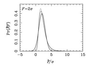
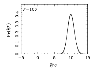
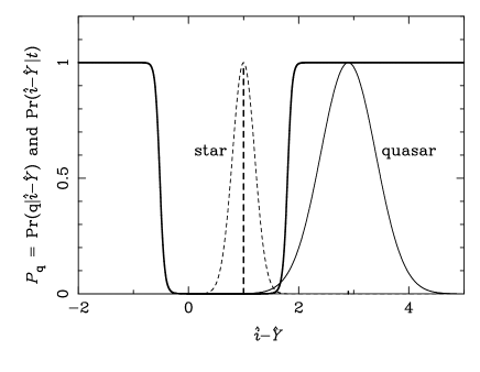
Given an estimated magnitude, $\hat{m}$, and an error $\Delta\hat{m}$, it is common to assume that the likelihood is Gaussian in magnitude units, and hence given by

$${\rm{Pr}}(\hat{m}|m)=\frac{1}{(2\pi)^{1/2}\,\Delta\hat{m}}\exp\left[-\frac{1}{2}\left(\frac{\hat{m}-m}{\Delta\hat{m}}\right)^{2}\right],$$ (27)

where $m$ is the true magnitude of the source in this band. Changing variables to flux units, the implied likelihood would then be

$${\rm{Pr}}(\hat{F}|F)$$

$$\mbox{}=\frac{1}{(2\pi)^{1/2}\,\Delta\hat{m}}\exp\left\{-\frac{1}{2}\left[\frac{m(\hat{F})-m(F)}{\Delta\hat{m}}\right]^{2}\right\}\left|\frac{{\mathrm{d}}m}{{\mathrm{d}}F}\right|,$$ (28)

where $m(F)$ and $|{\mathrm{d}}m/{\mathrm{d}}F|$ are given in Eqs (21) and (23) for logarithmic magnitudes and Eqs (24) and (26) for asinh magnitudes, respectively.

The resultant expressions for the likelihood are straightforward, but cumbersome; they are more easily explored visually, as is done in Fig. 12. For the brighter source with a true flux of $F=10\sigma$ (where $\sigma$ is the background noise in flux units) the Gaussian likelihoods in terms of both magnitudes are consistent with the true Gaussian in flux units, and of course almost any subsequent inferences would be similarly accurate. For the fainter sources with true fluxes of $F=0.1\sigma$ and $F=2\sigma$, however, the differences between the likelihood formaluations are readily apparent. Most importantly, negative measured fluxes cannot be represented in the traditional logarithmic magnitude system, rendering it useless in such low $S/N$ situations. The situation for asinh magnitudes is more complicated: with $m\propto F$ for small $|F|$, the likelihood in the $F=0.1\sigma$ case is fairly accurate; but, given the choice of softening parameter used here, the are significant differences in the $F=2\sigma$ case.

Any conclusions drawn from magnitude-based Gaussian likelihoods will be discrepant, and in some cases catastrophically so. In the case of the toy model adopted in Section A.1, using a Gaussian in magnitude units can result in nonsensical inferences, as shown in Fig. 13. The absurd rise of $P_{\mathrm{q}}$ to near unity for unusually blue sources (that are on the ‘far’ side of the stellar locus from the quasars) is because the weighted Gaussian in magnitude units for the brighter, well measured, stars is less than the down-weighted Gaussian for the fainter, less accurately measured, quasars. Despite the much lower prior for the quasars, the stars’ smaller error eventually dominates. The same calculation performed in flux units does not have this problem as, for these faint sources, the background error is the same for both in flux units. For extremely blue or red sources which are a bad fit to both models the likelihood is almost irrelevant and the prior is the dominant factor, as it should be.

Operationally, the solution to these potential complications is to convert magnitude data into flux units for the purposes of any likelihood-based calculations, the formulae for which are given below.

A.2.4 Magnitude to flux conversions

Given the importance of performing statistical calculations in flux units, formulae are needed to convert an estimated magnitude, $\hat{m}$, and its associated error, $\Delta\hat{m}$, into an estimated flux, $\hat{F}$, and, in the case of faint sources, the background noise, $\sigma$. The correct conversions can be derived from the fact that $\hat{m}$ and $\Delta\hat{m}$ are inevitably calculated from $\hat{F}$ and $\sigma$ in the first place. The problem would be more difficult if reported magnitudes and uncertainties were obtained using more complicated statistical arguments, but for the simple conversions commonly adopted all that is required is to invert the relationships in Sections A.2.1 and A.2.2.

Given $\hat{m}$ and $\Delta\hat{m}$ in conventional logarithmic magnitudes, a straightforward subsitution into Eq. (22) yields

$$\hat{F}=F_{0}\exp\left[-\frac{2\ln(10)}{5}\hat{m}\right].$$ (29)

Then using Eq. (23) gives

$$\sigma = F_{0}\frac{2\ln(10)}{5}\exp\left[-\frac{2\ln(10)}{5}\hat{m}\right]\Delta\hat{m}$$ (30)

$$= \hat{F}\frac{2\ln(10)}{5}\,\Delta\hat{m}\simeq\Delta\hat{m}\,\hat{F}.$$

Given $\hat{m}$ and $\Delta\hat{m}$ in terms of asinh magnitudes, the corresponding flux estimate is given from Eq. (25) yields

$$\hat{F}=2\times 10^{-2m_{0}/5}F_{0}\sinh\left[\frac{2\ln(10)}{5}(m_{0}-\hat{m})\right]$$ (31)

Then using Eq. (23) to change variables gives the background error in flux units as

$$\sigma=\frac{4\ln(10)}{5}10^{-2m_{0}/5}F_{0}\cosh\left[\frac{2\ln(10)}{5}(m_{0}-\hat{m})\right].$$ (32)

For the calculation of $P_{\mathrm{q}}$ in Section 3, Eqs (29) and (30) were used to convert the reported UKIDSS $Y$- and $J$-band photometry to flux units and Eqs (31) and (32) were used to convert the reported SDSS $i$- and $z$-band SDSS photometry to flux units.

Appendix B Parameter fitting for the stellar population model

In Section 3.2 it was necessary to fit the parameters of an empirical model of the intrinsic stellar colour and magnitude distribution to a sample of UKIDSS–SDSS point–sources extracted from the WSA. Many methods exist for tackling this problem, although the fact that the observed distribution is the result of convolving the underlying target distribution with magnitude-dependent noise makes this task non-trivial in this case. The overall theme of this paper would suggest taking a Bayesian approach, but the primary aim here is to find any function to describe the intrinsic stellar distribution that is consistent with the observed data; the actual parameter values (and their uncertainties) are not of interest. Hence a faster, if less principled, method was used.

After selecting $\sim 10^{5}$ bright, red UKIDSS–SDSS stars (with $\mbox{$\hat{i}$$-$$\hat{Y}$}\geq 2.0$ and $15.0\leq\hat{Y}\leq 19.5$), the sample was binned in $\hat{Y}$ and $\hat{i}$$-$$\hat{Y}$, with a bin size of 0.1. The data was hence reduced to the number of objects, $n_{i}$, in each of $N_{\mathrm{bin}}$ cells (where the index $i$ covers the two-dimensional parameter space). For a given choice of the free parameters, ${\phi}$, describing the model under consideration (as distinct from the parameters $\mbox{\boldmath${\theta}$}_{\mathrm{s}}$ used to characterise a single star), the expected number of stars in each cell, $\bar{n}_{i}(\mbox{\boldmath${\phi}$})$, was calculated by convolving the intrinstic population with the appropriate photometric error distribution. It also important to ensure that the value of $\bar{n}_{i}(\mbox{\boldmath${\phi}$})$ is not spuriously high due to the large number of faint undetected sources that could, at least in theory, be scattered into the bin. The potential problem with a simple treatment is that such numerous faint sources are typically beyond the confusion limit of the survey and so to treat a single noise spike as being associated with each in turn results in an unrealistically high probability of a spurious source entering the survey. The key is to adopt a self-consistent treatment in which sources at or below the confusion limit are ignored (cf. Mortlock 2009).

Irrespective of the method by which $\bar{n}_{i}(\mbox{\boldmath${\phi}$})$ is calculated, $n_{i}$ is Poisson-distributed and uncorrelated between bins. The log-likelihood of the full data-set is hence

$$\ln[{\rm{Pr}}(\mbox{\boldmath${n}$}|\mbox{\boldmath${\phi}$})] = \ln\left\{\prod_{i=1}^{N_{\mathrm{bin}}}\frac{[\bar{n}_{i}(\mbox{\boldmath${\phi}$})]^{n_{i}}\exp[-\bar{n}_{i}(\mbox{\boldmath${\phi}$})]}{n_{i}!}\right\}$$

$$= \sum_{i=1}^{N_{\mathrm{bin}}}n_{i}\ln[\bar{n}_{i}(\mbox{\boldmath${\phi}$})]-\bar{n}_{i}(\mbox{\boldmath${\phi}$})+{\mathrm{constant}}.$$

The best fit parameters given in Eq. (9) were found by minimizing Eq. (B) using the downhill simplex method Press et al. (2007).

References

- Abazajian et al. (2009) Abazajian K. N., et al., 2009, ApJS, 182, 543
- Bailer-Jones et al. (2008) Bailer-Jones C. A. L., Smith K. W., Tiede C., Sordo R., Vallenari A., 2008, MNRAS, 391, 1838
- Barkana & Loeb (2001) Barkana R., Loeb A., 2001, Phys. Rep., 349, 125
- Becker et al. (2001) Becker R. H., Fan X., White R. L., et al. 2001, AJ, 122, 2850
- Benítez (2000) Benítez N., 2000, ApJ, 536, 571
- Bovy et al. (2010) Bovy J., et al., 2010, ApJ, submitted
- Casali et al. (2007) Casali M., et al., 2007, A&A, 467, 777
- Dunkley et al. (2009) Dunkley J., et al., 2009, ApJS, 180, 306
- Dye et al. (2006) Dye S., et al., 2006, MNRAS, 372, 1227
- Emerson et al. (2004) Emerson J. P., Sutherland W. J., McPherson A. M., Craig S. C., Dalton G. B., Ward A. K., 2004, The Messenger, 117, 27
- Fan et al. (2006) Fan X., et al., 2006, AJ, 132, 117
- Fan et al. (2004) Fan X., Hennawi J. F., Richards G. T., et al. 2004, AJ, 128, 515
- Fan et al. (2001) Fan X., Narayanan V. K., Lupton R. H., et al. 2001, AJ, 122, 2833
- Fan et al. (2002) Fan X., Narayanan V. K., Strauss M. A., White R. L., Becker R. H., Pentericci L., Rix H.-W., 2002, AJ, 123, 1247
- Fan et al. (2003) Fan X., Strauss M. A., Schneider D. P., et al. 2003, AJ, 125, 1649
- Fukugita et al. (1996) Fukugita M., Ichikawa T., Gunn J. E., Doi M., Shimasaku K., Schneider D. P., 1996, AJ, 111, 1748
- Gehrels et al. (2009) Gehrels N., Ramirez-Ruiz E., Fox D. B., 2009, ARA&A, 47, 567
- Glikman et al. (2008) Glikman E., Eigenbrod A., Djorgovski S. G., Meylan G., Thompson D., Mahabal A., Courbin F., 2008, AJ, 136, 954
- Gunn & Peterson (1965) Gunn J. E., Peterson B. A., 1965, ApJ, 142, 1633
- Hambly et al. (2008) Hambly N. C., et al., 2008, MNRAS, 384, 637
- Hazard et al. (1963) Hazard C., Mackey M. B., Shimmins A. J., 1963, Nature, 197, 1037
- Hewett et al. (1995) Hewett P. C., Foltz C. B., Chaffee F. H., 1995, AJ, 109, 1498
- Hewett et al. (2006) Hewett P. C., Warren S. J., Leggett S. K., Hodgkin S. T., 2006, MNRAS, 367, 454
- Ivezić et al. (2004) Ivezić Ž., et al., 2004, IAUS, 222, 525
- Jaynes (2003) Jaynes E. T., 2003, Probability Theory. Cambridge University Press, Cambridge, UK
- Jiang et al. (2008) Jiang L., et al., 2008, AJ, 135, 1057
- Jiang et al. (2009) Jiang L., Fan X., Bian F., Annis J., Chiu K., Jester S., Lin H., Lupton R. H., Richards G. T., Strauss M. A., Malanushenko V., Malanushenko E., Schneider D. P., 2009, AJ, 138, 305
- Kaiser et al. (2002) Kaiser N., et al., 2002, in Tyson J. A., Wolff S., eds, Society of Photo-Optical Instrumentation Engineers (SPIE) Conference Series Vol. 4836 of Society of Photo-Optical Instrumentation Engineers (SPIE) Conference Series. p. 154
- Lawrence et al. (2007) Lawrence A., et al., 2007, MNRAS, 379, 1599
- Lupton et al. (1999) Lupton R. H., Gunn J. E., Szalay A. S., 1999, AJ, 118, 1406
- Maddox et al. (2008) Maddox N., Hewett P. C., Warren S. J., Croom S. M., 2008, MNRAS, 386, 1605
- Mortlock (2009) Mortlock D. J., 2009, in Hobson M. P., Jaffe A. H., Liddle A., Mukherjee P., Parkinson D., eds, Bayesian Methods In Cosmology Cambridge University Press, p. 193
- Mortlock et al. (2009) Mortlock D. J., et al., 2009, A&A, 505, 97
- Mortlock et al. (2011) Mortlock D. J., Patel M., Warren S. J., Venemans B. P., Hewett P. C., McMahon R. G., Simpson C. J., Sharp R. G., 2011, MNRAS, in preparation
- Mortlock et al. (2009) Mortlock D. J., Peiris H. V., Ivezić Ž., 2009, MNRAS, 399, 699
- Patel et al. (2011) Patel M., et al., 2011, MNRAS, in preparation
- Pogson (1856) Pogson N., 1856, MNRAS, 17, 12
- Press et al. (2007) Press W. H., Teukolsky S. A., Vetterling W. T., Flannery B. P., 2007, Numerical Recipes: The Art Of Scientific Computing (3rd Ed.). Cambridge University Press
- Richards et al. (2004) Richards G. T., et al., 2004, ApJS, 155, 257
- Richards et al. (2009) Richards G. T., et al., 2009, AJ, 137, 3884
- Schmidt (1963) Schmidt M., 1963, Nature, 197, 1040
- Schmidt et al. (1995) Schmidt M., Schneider D. P., Gunn J. E., 1995, AJ, 110, 68
- Schneider (1999) Schneider D. P., 1999, in Holt S., Smith E., eds, After the Dark Ages: When Galaxies were Young (the Universe at ) Vol. 470 of American Institute of Physics Conference Series, Surveys for High-redshift Quasars. p. 233
- Scranton et al. (2005) Scranton R., Connolly A. J., Szalay A. S., Lupton R. H., Johnston D., Budavari T., Brinkman J., Fukugita M., 2005, AJ, submitted
- Sivia & Skilling (2006) Sivia D. S., Skilling J., 2006, Data Analysis: A Bayesian Tutorial. Oxford University Press, Oxford, UK
- Skrutskie et al. (2006) Skrutskie M. F., et al., 2006, AJ, 131, 1163
- Stark et al. (2010) Stark D. P., Ellis R. S., Chiu K., Ouchi M., Bunker A., 2010, MNRAS, 408, 1628
- Venemans et al. (2011) Venemans B. P., et al., 2011, MNRAS, in preparation
- Venemans et al. (2007) Venemans B. P., McMahon R. G., Warren S. J., Gonzalez-Solares E. A., Hewett P. C., Mortlock D. J., Dye S., Sharp R. G., 2007, MNRAS, 376, L76
- Warren et al. (2007) Warren S. J., et al., 2007, MNRAS, 375, 213
- Warren et al. (1994) Warren S. J., Hewett P. C., Osmer P. S., 1994, ApJ, 421, 412
- Willott et al. (2007) Willott C. J., et al., 2007, AJ, 134, 2435
- Willott et al. (2010) Willott C. J., et al., 2010, AJ, 139, 906
- Wyithe (2008) Wyithe J. S. B., 2008, MNRAS, 387, 469
- York et al. (2000) York D. G., et al., 2000, AJ, 120, 1579