Efficiently enclosing the compact binary parameter space by singular-value decomposition

Abstract

Gravitational-wave searches for the merger of compact binaries use matched-filtering as the method of detecting signals and estimating parameters. Such searches construct a fine mesh of filters covering a signal parameter space at high density. Previously it has been shown that singular value decomposition can reduce the effective number of filters required to search the data. Here we study how the basis provided by the singular value decomposition changes dimension as a function of template bank density. We will demonstrate that it is sufficient to use the basis provided by the singular value decomposition of a low density bank to accurately reconstruct arbitrary points within the boundaries of the template bank. Since this technique is purely numerical it may have applications to interpolating the space of numerical relativity waveforms.

I Introduction

Several broadband laser interferometer gravitational-wave (GW) detectors are operating at high sensitivities and will continue to improve over the next decade The LIGO Scientific Collaboration (2009); The Virgo Scientific Collaboration (2005); Grote and the LIGO Scientific Collaboration (2010); et al (2008); Collaboration (2009). As detectors improve it is increasingly likely that GW astronomers will observe gravitational radiation emitted from the coalescence of compact binary systems involving neutron stars and or stellar mass black holes Collaboration (2010).

Because compact binary coalescence (CBC) waveforms are well modeled, GW searches for such signals are conducted by matched filtering the detectors’ data with banks of template waveforms, chosen to adequately cover a region of the signal parameter space Owen (1996). For GW signals from the merger of compact objects with negligible spin, this parameter space is defined by functions of the masses of the two objects. To search for signals within this parameter space, a bank of templates is constructed to sample the parameter space sufficiently densely such that there is minimal loss of signal-to-noise ratio (SNR). Traditionally, template banks used to search this two-dimensional signal parameter space have been constructed using the $(A_{2})^{*}$ lattice Cokelaer (2007), referred to as “hexagonally-placed” template banks. This problem becomes more difficult in higher dimensions, where other types of template placement algorithms have recently been investigated Harry et al. (2009); Manca and Vallisneri (2010); Messenger et al. (2009); Prix (2007).

In Cannon et al. (2010) the singular value decomposition (SVD) was applied to CBC waveforms to show how hexagonally-placed template banks with $M$ templates could be implemented with $N^{\prime}\ll 2M$ filters ($2M$ being the nominal number of filters required for the $M$ 2-phase templates). This was achieved by truncating the SVD of the matrix consisting of the time-series of the template waveforms. Here we demonstrate that the bases identified by the SVD is effective at spanning the space of all CBC waveforms within the region of parameter space sampled by the original bank. We find that the SVD of a low-density bank provides a basis suitable for constructing all the waveforms from a higher-density bank, even waveforms at arbitrary locations within that region of parameter space.

This paper is organized as follows. Sec. II describes how we apply the SVD to approximately embed the signal manifold in a vector space. Sec. III tests this embedding by reconstructing various points in the manifold. Finally, Sec. IV discusses possible applications of this technique.

II Enclosing the signal space with Singular Value Decomposition

In this section we explore how the number of basis vectors required to reconstruct a template bank scales with the initial density of the template bank. We define a template bank of signal waveforms covering a patch $\mathcal{P}$ of the signal manifold, which is used to test for the presence and strength of signals from $\mathcal{P}$ in the detectors’ data. We construct a signal matrix in the same manner as Cannon et al. (2010). Specifically, we create a real-valued matrix ${\bf H}$ by alternately filling its rows with the real and imaginary parts (cosine and sine) of the template waveform time series from a CBC template bank covering $\mathcal{P}$, ${\bf H}=\{H_{\alpha j}\}=\{\Re\vec{h}_{1},\Im\vec{h}_{1},\Re\vec{h}_{2},\Im\vec{h}_{2},...,\Re\vec{h}_{M},\Im\vec{h}_{M}\}^{\mathrm{T}}$.

As in Cannon et al. (2010), we constructed the template matrix with chirp masses $M_{c}=M\eta^{5/6}$, where $M=m_{1}+m_{2}$ is the total mass and $\eta=m_{1}m_{2}/M^{2}$ is the symmetric mass ratio, of $1.125M_{\odot}\leq M_{c}<1.240M_{\odot}$ and component masses of $1M_{\odot}\leq m_{1},m_{2}<3M_{\odot}$. Template banks covering this region are created using template placement algorithms of the LIGO Algorithms Library LIGO Scientific Collaboration . Template placement is done in the $(\tau_{0},\tau_{3})$ plane, where $\tau_{0}$ and $\tau_{3}$ are defined as

$$\tau_{0}=\frac{5}{256}\left(\pi f_{0}\right)^{-8/3}M_{c}^{-5/3},$$ (1)

$$\tau_{3}=\frac{\pi}{8}\left(\pi f_{0}\right)^{-5/3}M_{c}^{-2/3}\eta^{-3/5},$$ (2)

and where $f_{0}$ is some fiducial frequency, which we choose to be $f_{0}=60$ Hz.

The non-spinning waveforms for each template are produced to 3.5 post-Newtonian (PN) order, sampled at 2048 Hz, up to the Nyquist frequency of 1024 Hz. The last 10 seconds of each waveform, whitened with the initial LIGO amplitude spectral density, are used to construct ${\bf H}$. The SVD is then applied to ${\bf H}$, decomposing the matrix into two unitary matrices, ${\bf V}$ and ${\bf U}$, and a diagonal matrix ${\bf\Sigma}$

$${\bf H}={\bf V}{\bf\Sigma}{\bf U}^{\mathrm{T}},$$ (3)

where ${\bf U}$ is a matrix composed of basis vectors (i.e., unit-norm time-series vectors), ${\bf V}$ is a matrix composed of reconstruction coefficients, and ${\bf\Sigma}$ is a matrix containing the singular values of ${\bf H}$.

In Cannon et al. (2010), it was demonstrated that truncating the reconstruction of ${\bf H}$ to use only the $N^{\prime}$ basis vectors with the largest singular values results in an average fractional SNR loss $\left\langle\delta\rho/\rho\right\rangle$ proportional to the sum of the discarded singular values squared. In this investigation, we truncate these reconstruction matrices at $\left\langle\delta\rho/\rho\right\rangle=10^{-7}$. This corresponds roughly to the truncation error of IEEE 754 32-bit floating-point numbers.

Figure 1: The number of filters as a function of minimal match, which increases with the density of the template bank. The total number of filters in the template bank, $N$, is shown by the dashed line. The number of filters needed to reconstruct the template matrix such that $\langle\delta\rho/\rho\rangle=10^{-7}$, $N^{\prime}$, is shown by the solid line. We find that the number filters needed to reconstruct ${\bf H}$ saturates when the minimal match reaches $\sim 89.9\%$.

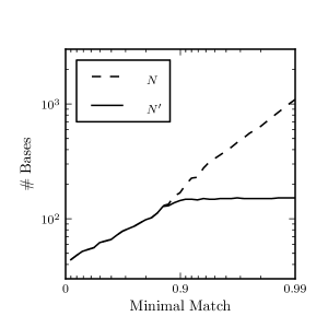
We explore how the number of basis vectors changes as the number of rows in ${\bf H}$ is increased by generating template banks for $\mathcal{P}$ with increasing density (i.e., increasing minimal match). We confirmed that the number of basis vectors required to reconstruct ${\bf H}$ saturates at a particular value of minimal match. Fig. 1 shows that as the minimal match of the template bank is increased, resulting in denser samplings of $\mathcal{P}$, the number of basis vectors needed to reconstruct ${\bf H}$ to the required accuracy saturates around a minimal match of $\sim 89.9\%$. This indicates that $\mathcal{P}$ is able to be embedded—to an accuracy of 1 part in $10^{7}$—in a vector space consisting of $\sim 150$ dimensions.

In the next section we will demonstrate how the basis waveforms identified by the coarsely sampled bank can be used to reconstruct templates at arbitrary points on the signal manifold.

III Efficient reconstruction of waveforms in the manifold

In order to determine how well these waveforms can be reconstructed, we compute a quantity called the average fractional SNR loss $\delta\rho_{\alpha}/\rho_{\alpha}$. This quantity can be thought of as the mismatch between the original waveform $\vec{h}_{\alpha}$ and the reconstructed waveform $\vec{h}^{\prime}_{\alpha}$, averaged over the phase angle. It tells us how far the reconstructed waveform is from the original waveform. As in Eq. (25) of Cannon et al. (2010), $\delta\rho_{\alpha}/\rho_{\alpha}$ is given in terms of SVD quantities as

$$\frac{\delta\rho_{\alpha}}{\rho_{\alpha}}=\frac{1}{4}\sum_{\mu=N^{\prime}+1}^{N}\left(v_{(2\alpha-1)\mu}^{2}+v_{(2\alpha)\mu}^{2}\right)\sigma_{\mu}^{2},$$ (4)

where $v_{(2\alpha-1)\mu}$ and $v_{(2\alpha)\mu}$ are the reconstruction coefficients for the real and imaginary parts, respectively, of the $\alpha$th waveform associated with the $\mu$th basis vector and are elements of ${\bf V}$, $\sigma_{\mu}$ is the $\mu$th element of ${\bf\Sigma}$, and the sum is over the truncated terms of ${\bf V}$ and ${\bf\Sigma}$.

Figure 2: A visual representation showing the two types of points of $\mathcal{P}$ that we can choose to reconstruct. The left cartoon shows an example point that is in ${\bf H}$, and thus in $\mathcal{P}$. The right cartoon shows an example point that is not part of H but is in $\mathcal{P}$.

We test this embedding of the signal manifold to see how well various points in the manifold can be reconstructed. The tests points we reconstruct are of two types: 1) those from the original signal matrix ${\bf H}$, 2) those absent from ${\bf H}$ but within $\mathcal{P}$. These two types of tests are illustrated in Fig. 2.

Figure 3: A histogram of the reconstruction accuracy of the waveforms that went into the construction of ${\bf H}$. As expected, the average reconstruction (solid line) accuracy matches the expected fractional SNR loss (dashed line).

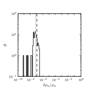
A test of the first type is shown in Fig. 3. This shows that the average reconstruction accuracy for points from ${\bf H}$ agrees with our chosen value of $10^{-7}$. This result is expected as it is an extension of the investigation from Fig. 4 of Cannon et al. (2010) applied to a more stringent reconstruction accuracy.

Figure 4: (left) A histogram of the mismatch between waveforms from $\mathcal{P}$ that were not in ${\bf H}$ and their reconstructed versions. The peak of the mismatch is slightly above the expected fractional SNR loss for waveforms from ${\bf H}$ (dashed line). (right) How the mismatch varies across $\mathcal{P}$, averaged across the $\tau_{3}$ direction. The largest mismatches come from near the borders of the template bank in the $\tau_{0}$ direction. Fig. 5 restricts our attention to the central $75\%$ of the domain of $\mathcal{P}$, whose boundaries are shown as vertical dotted lines.

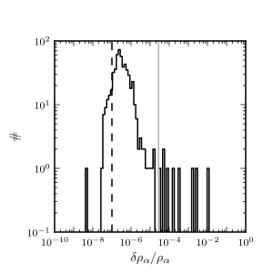
A test of the second type is shown in Fig. 4. To choose points uniformly from $\mathcal{P}$ but absent from ${\bf H}$, we generate a denser template bank within the same region of parameter space described in the Sec. II. Specifically, we generate this template bank with a minimal match of $99\%$. In order to test the reconstruction accuracy of these waveforms, we project the real and imaginary parts of the waveforms onto the basis vectors from the SVD of ${\bf H}$

$$v^{\prime}_{\alpha\mu}=\frac{1}{\sigma_{\mu}}\sum_{j}h_{\alpha j}u_{\mu j},$$ (5)

where $v^{\prime}_{\alpha\mu}$ represents a reconstruction coefficient associated with the $\mu$th basis vector for the real or imaginary part of the $\alpha$th waveform from the denser template bank, $\sigma_{\mu}$ is the $\mu$th element of ${\bf\Sigma}$, $h_{\alpha j}$ is the $j$th time sample of the real or imaginary part of the $\alpha$th waveform from the denser template bank, and $u_{\mu j}$ is the $j$th time sample from the $\mu$th basis vector in ${\bf U}$. The real and imaginary parts of the waveforms from the denser template bank are then reconstructed using

$$h^{\prime}_{\alpha j}=\sum_{\mu}v^{\prime}_{\alpha\mu}\sigma_{\mu}u_{\mu j}\,.$$ (6)

Figure 5: Similar plots as in Fig. 4, eliminating test points near the boundaries in the $\tau_{0}$ direction. (left) A histogram of the mismatch between waveforms from $\mathcal{P}$ that were not in ${\bf H}$ and their reconstructed versions. The average reconstruction (solid line) accuracy is slightly worse than the expected fractional SNR loss (dashed line).

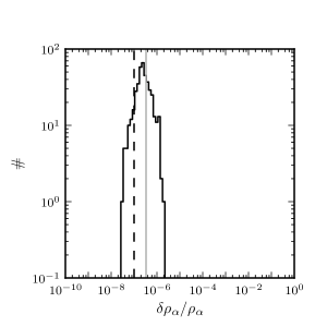
The distribution of $\delta\rho_{\alpha}/\rho_{\alpha}$ for these waveforms, left panel of Fig. 4, shows a tail extending to large mismatches. Examining where these large mismatches are located in parameter space, we find they originate from near the boundaries of $\mathcal{P}$. Removing the test points near the boundaries in the $\tau_{0}$ direction, shown in Fig. 5, we find the tail of large mismatches disappears.

Figure 6: (left) A plot showing a smaller region of $\mathcal{P}$. The circles are points whose waveforms go into ${\bf H}$. The line segment $\overline{AB}$ connects one of those points, $A$, with the point $B$, the central point of $A$ and two of its nearest neighbors. Point $B$ is situated such that it should have a $89.9\%$ fitting factor with each of the surrounding points. (right) How well a waveform from a given point of $\overline{AB}$, $\vec{h}_{p}$, can be “matched”. The Match shows the normalized inner-product between $\vec{h}_{A}$ and the waveform from the corresponding point along $\overline{AB}$. The Fitting Factor shows the same match maximized over phase and time. Since we are using a $89.9\%$ minimal match bank, it is expected that the fitting factor falls to around that value. The SVD Projection is given by $1-\delta\rho_{\alpha}/\rho_{\alpha}$. The SVD basis vectors are able to reconstruct to high accuracy all points along the line.

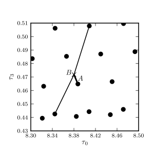
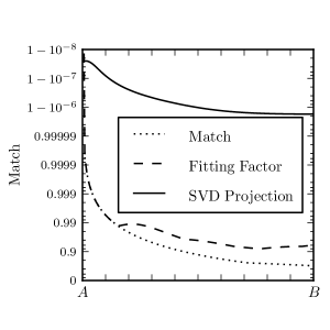
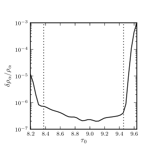
An additional test of the second type, which systematically explores the reconstruction accuracy near a point whose waveform went into ${\bf H}$, is shown in Fig. 6. The left panel shows a set of three nearest-neighbor templates. We investigate how the reconstruction accuracy varies as one moves from point $A$ to the central point, point $B$. Point $B$ is assumed to have the largest mismatch between its waveform and the waveforms from any of the three surrounding points. We also compute the mismatch between the waveforms along $\overline{AB}$ and the waveform of point $A$ with and without maximizing over phase and time, called the fitting factor and match respectively. The fitting factor falls to the minimal match of the template bank when comparing the waveforms from $A$ and $B$, which is expected as the minimal match involves maximizing over phase and time. The reconstruction accuracy associated with SVD projection is consistently high and close to the chosen reconstruction accuracy of 1 part in $10^{7}$.

IV Discussion

These investigations show that the SVD can be used to find a set of basis vectors that not only span the signal matrix ${\bf H}$, but also enclose the signal manifold $\mathcal{P}$ sampled by ${\bf H}$.

GW pipelines that search for known waveforms, such as GWs from CBCs, commonly compute waveform consistency statistics that compare the observed response of a template waveform filter to the data with what one would expect given the presence of that signal. These consistency statistics are found to perform better when the mismatch between the template waveform and the signal waveform is small Allen (2005). Filtering with a fixed density template bank can introduce mismatch between the nearest template and the signal. This mismatch can be greatly reduced if one is able to find the exact point in parameter space where the signal is located and filter the data using that point. Using the SVD basis vectors, one could reconstruct a point closer to the point of the signal and improve the waveform consistency statistics.

Parameter estimation techniques for GWs from CBCs often use Monte Carlo Markov Chain algorithms to search the parameter space. This involves producing waveforms and filtering the data against many points of the parameter space. The SVD could also be used to interpolate waveforms that are expensive to compute, as in the case of waveforms produced by solving differential equations. Also, if one filtered the data using the basis vectors from the SVD, it would be very easy to reconstruct to high accuracy the output one would see if one had filtered the data using a waveform from anywhere within the parameter space.

In order to gain benefit from these applications, it would be necessary to determine the reconstruction coefficients in a computationally efficient manner. This work has not tried to address this problem as: 1) it has assumed the target waveforms are known, and 2) it computes the reconstruction coefficients using computationally expensive inner products. Generation of these reconstruction coefficients warrants future investigation as the benefits derived from this technique would be substantial.