Quantum transport of double quantum dots coupled to an oscillator in arbitrary strong coupling regime

Abstract

In this paper, we investigate the quantum transport of a double quantum dot coupled with a nanomechanical resonator at arbitrary strong electron-phonon coupling regimes. We employ the generalized quantum master equation to study full counting statistics of currents. We demonstrate the coherent phonon states method can be applied to decouple the electron-phonon interaction non-perturbatively. With the help of this non-perturbative treatment of electron-phonon couplings, we find that the phonon-assisted resonant tunneling emerges when the excess energy from the left quantum dot to the right one can excite integer number of phonons and multi-phonon excitations can enhance the transport in strong electron-phonon coupling regime. Moreover, we find that as the electron-phonon coupling increases, it first plays a constructive role to assist the transport, and then plays the role of scattering and strongly represses the transport.

1 Introduction

With the increasing promotion of nanotechnology, people now have the abilities to fabricate fertile atomic and molecular quantum devices, such as single superconducting electron transistors Fulton , quantum dots Ashoori and single molecular transistors SMT . As a consequence, great attentions have recently been attracted on research fields of molecular electronics Aviram ; Joachim ; Bumm ; Reed and nanoelectromechanical systems Craighead ; Cleland ; Blencowe , because of their immense potentials to bridge scientific researches and industry applications. One of such promising devices is Double Quantum Dot (DQD) system Jong1 , which, as artificial atoms, is able to confine one or several electrons to form effective two level system, so as to manipulate and control coherent transport of qubits by superposition of individual electrons’ natural states  Nakamura ; Vion ; Chiorescu ; Yu .

It was initially observed by Fujisawa et al. experimentally Fujisawa and then explained by Brandes et al. theoretically Brandes1 that single electron tunneling on such quantum dots system inevitably interplays with its environment, such as electron-phonon (e-ph) interaction due to vibrations of the system. The transport properties are extremely sensitive to the motion of the nanomechanical resonator such that they can be also utilized, in a reverse way, as detectors with high precisions for the quantization of the resonator positions Blencowe ; Knoibel ; Lahaye ; Naik ; Clerk . Therefore, it is definitely important to unravel the underlying interplay effect between electronics and vibrations on transport properties for future quantum technology development.

In the other hand, the main transport property, current, has been extensively studied in the past decades. However, current noise is not yet fully exploited as a powerful tool to extract more information to understand how the environment affects the transport GK1 ; Sanchez2008 . Especially, at low temperatures, shot noise Blanter is the main source contributing to current fluctuations because of the discreteness of transferring qubits and charges. Full counting statistics (FCS) Nazarov2 , initially proposed by Levitov et al. Levitov1 in mesoscopic physics, is proved as a splendid diagnostic tool to investigate complete information of quantum fluctuations both in calculations Sun ; bargrets1 ; Aguado1 ; bargrets2 ; Ren and measurements Wei1 ; Bylander ; Gustavsson . The main idea of FCS is, by introducing auxiliary counting parameters, to evaluate the cumulant generating function of probability distribution of transmitted charges. Current and shot noise are just the first two cumulants. The higher order cumulants indeed show more details to expand our views to study quantum fluctuation effects petter2011 ; Flindt ; Flindt2 . The underlying mathematics of FCS is named large deviation theory LDT1 , which has been widely used in various fields LDT2 ; LDT3 .

In this paper, we focus on effects of quantized vibrations of the nanomechanical resonator on transport properties of the DQD with large voltage bias between two electrodes. The vibration is specified by a single phonon mode, which interacts with an external thermal phonon environment. We derive a generalized quantum master equation (QME) including auxiliary counting parameters under the Born-Markov approximation and second-order perturbation of system-bath couplings. Though two-level system strongly coupled to the oscillator was studied intensively, people usually applied rotating wave approximation (RWA) or only investigated the ground state by variational methods in the closed systems irish1 ; hwang1 . While extended coherent phonon states method Chen1 ; Chen2 is adopted to capture the characteristics of excitations mixed by electrons and phonons with arbitrary strong e-ph coupling in the absence of RWA. This non-perturbative approach renders us beyond the previous perturbation expansion method by assuming a weak e-ph coupling Lambert1 . In fact, the strong e-ph interaction has already been found in carbon based nanoscale devices, shown in Refs. strongep1 ; strongep2 ; strongep3 . In recent quantum electrodynamics experiments, the coupling of the two-level artificial atom and the resonator also reaches the strong regime strongep4 . Therefore, our work about coherent phonon states approach, which is capable of dealing with arbitrary e-ph coupling strengths, is important and favorite.

The organization of this paper is as follows: we begin by modeling the system with generalized QME combined with coherent phonon states approach in the framework of FCS in section II. Details about how coherent phonon states can optimally decouple e-ph interaction non-perturbatively will be given there. In section III, results and discussions are presented, of which the first three cumulants of probability distribution of transmitted charges are scrutinized in the full range of e-ph coupling strengths. Finally, summary is given in section IV.

2 Theory and Methods

In this section, we first describe the whole Hamiltonian and then give the derivation of the generalized QME accompanied by auxiliary counting parameter and FCS. Finally, extended coherent phonon states approach will be articulated to show its ability to decouple the e-ph interaction.

2.1 The Whole Hamiltonian

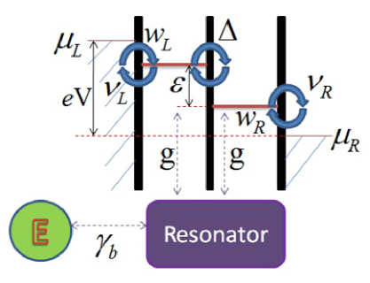
Figure 1: (Color online) Sketch map of the DQD (among three vertical thick lines, specified by two horizontal lines) coupled with the nanomechanical resonator (rectangle). Left and right areas with slash lines denote electrodes. The thermal environment of phonons is depicted by E (circle).

Hamiltonian of the whole system, as illustrated in Fig. 1, is generally described by

$$H=H_{S}+H_{\mathrm{Lead}}+H_{\mathrm{E}}+V_{\mathrm{DL}}+V_{\mathrm{RE}},$$ (1)

where $H_{S}$ denotes the coupled system of DQD and nanomechanical resonator. $H_{\mathrm{Lead}}$ depicts the two electrodes. $H_{\mathrm{E}}$ is the environment. $V_{\mathrm{DL}}$ describes the coupling between DQD and leads, while $V_{\mathrm{RE}}$ denotes the coupling between resonator and thermal environment. Their detailed expressions are to be explained in the following.

We assume only one electron is allowed to stay in DQD at most, considering strong coulomb repulsion in quantum dots. The system of the DQD coupled with a quantized nanomechanical resonator thus is expressed as:

$$~{}H_{S}=\frac{\varepsilon}{2}\sigma_{z}+\Delta\sigma_{x}+g\sigma_{z}(a^{\dagger}+a)+\omega_{b}a^{{\dagger}}a.$$ (2)

${\sigma}_{z}=|L\rangle\langle{L}|-|{R}{\rangle}{\langle}R|$ and $\sigma_{x}=|L{\rangle}{\langle}R|+|R{\rangle}{\langle}L|$, where $|L\rangle$ ($|R\rangle$) is the state of electron occupying left (right) dot. $\varepsilon$ means the energy level mismatch between quantum dots which can be tuned by gate voltage. $\Delta$ is the corresponding tunneling element between two quantum dots. $g$ is the dots-resonator (e-ph) coupling strength. $\omega_{b}$ denotes the quantized mode of the resonator and $a^{\dagger}$ $(a)$ depicts the corresponding phonon creator (annihilator).

The DQD is connected with two electrodes, described by $H_{\mathrm{Lead}}=\sum_{j=\{L,R\},k}\epsilon^{j}_{k}{c^{\dagger}_{jk}}c_{jk}$ with $\epsilon^{j}_{k}$ the electronic energy with momentum $k$ in $j$ electrode, and $c^{{\dagger}}_{jk}(c_{jk})$ creating (annihilating) the corresponding electrons. The Hamiltonian of electrode coupling parts is given as $V_{\mathrm{DL}}=\sum_{j=\{L,R\},k}{\eta}^{j}_{k}|j{\rangle}{\langle}0|c_{jk}+\textrm{H.c.}$, where ${\eta}^{j}_{k}$ is the coupling strength between DQD and $j$ electrode, and $|0\rangle$ denotes the empty electron state of DQD. The resonator is damped by external thermal environment, $H_{\mathrm{E}}=\sum_{k}\omega_{k}b^{\dagger}_{k}b_{k}$ with $\omega_{k}$ the phonon frequency and $b^{\dagger}_{k}(b_{k})$ the corresponding creator (annihilator). The damping Hamiltonian is described by $V_{\mathrm{RE}}=\sum_{k}\lambda_{k}{a^{\dagger}}b_{k}+\textrm{H.c.}$, where $\lambda_{k}$ denotes the coupling of resonator and the thermal environment with phonon in momentum $k$. Without loss of generality, we set $\hbar=1,k_{B}=1$, $e=1$ and $\omega_{b}=1$ as the energy unit.

2.2 Generalized QME and FCS

To measure fluctuations of electron current through the right electrode, we add the counting term to the whole Hamiltonian as Esposito :

$$~{}H_{\chi} = e^{\frac{i}{2}{\chi}N_{R}}He^{-\frac{i}{2}{\chi}N_{R}}$$ (3)

$$= H_{S}+H_{\mathrm{Lead}}+H_{\mathrm{E}}+V_{\mathrm{RE}}+V_{\mathrm{DL}}(\chi),$$

where $V_{\mathrm{DL}}(\chi)$ is transformed from the original $V_{\mathrm{DL}}$, reading:

$$V_{\mathrm{DL}}(\chi)=\sum_{k}\left(e^{-\frac{i}{2}\chi}{\eta}^{R}_{k}|R{\rangle}{\langle}0|c_{Rk}+{\eta}^{L}_{k}|L{\rangle}{\langle}0|c_{Lk}\right)+\textrm{H.c.},$$

and $N_{R}=\sum_{k}c^{{\dagger}}_{Rk}c_{Rk}$ is the electron number operator in right electrode. $\chi$ is the auxiliary counting parameter in FCS, appearing in the right coupling part of $V_{\mathrm{DL}}(\chi)$ to count the electron number into the right electrode.

Following the standard procedure, we treat $V_{\chi}=V_{\mathrm{RE}}+V_{\mathrm{DL}}(\chi)$ as the perturbation. Note here, the couplings between the system $H_{S}$ and its environments are required to be weak, but not the e-ph coupling $g$ inside $H_{S}$. Actually, $g$ can be arbitrary strong, compared to the energy scale $\omega_{b}$. In this way, under Born-Markov approximation, the modified QME is derived up to the second order of $V_{\chi}$ Esposito :

$$\frac{d\rho^{S}_{\chi}(t)}{dt} = -i[H_{S},\rho^{S}_{\chi}(t)]$$ (4)

$$-\int^{\infty}_{0}d\tau\langle[V_{\chi},[V_{\chi}(-\tau),\rho_{\chi}(t)]_{\chi}]_{\chi}{\rangle}_{\textrm{E,Lead}},$$

where $[A_{\chi},B_{\chi}]_{\chi}=A_{\chi}B_{\chi}-B_{\chi}A_{-\chi}$ for abbreviation, and $\rho^{S}_{\chi}=\textrm{Tr}_{\mathrm{E,Lead}}(\rho_{\chi})$ is the reduced system density matrix composed of DQD and resonator, by tracing out degrees of freedom in electrode leads and thermal environment.${\langle}O{\rangle}_{\textrm{E,Lead}}$ shows thermal average of $O$ over the thermal reservoir E and two electrode leads. The detail derivation of Eq. (4) can be found in Appendix A. Note that $\rho^{S}_{\chi}$ is a twisted density matrix by the counting parameter $\chi$. When $\chi=0$, $\rho^{S}_{\chi}$ reduces to the conventional density matrix. Therefore, for the system considered here, we finally obtain the evolution equation of $\rho^{S}_{\chi}$, as:

$$\frac{d}{dt}{\rho^{S}_{\chi}} = -i[H_{S},\rho^{S}_{\chi}]+L_{e}[\rho^{S}_{\chi}]+L_{a}[\rho^{S}_{\chi}],$$ (5)

where $L_{e}[\rho^{S}_{\chi}]=$

$$-\sum_{j=\{L,R\};{n,m}}\bigg{(}{\nu_{j}}(\epsilon_{nm})\left(\rho^{S}_{\chi}|n{\rangle}{\langle}n|S^{{\dagger}}_{j}|m{\rangle}{\langle}m|S_{j}+\textrm{H.c.}\right)\\ +w_{j}(\epsilon_{nm})\left(S_{j}|n{\rangle}{\langle}n|S^{{\dagger}}_{j}|m{\rangle}{\langle}m|\rho^{S}_{\chi}+\textrm{H.c.}\right)\\ -w_{j}(\epsilon_{nm})\left(|n{\rangle}{\langle}n|S^{{\dagger}}_{j}|m{\rangle}{\langle}m|\rho^{S}_{\chi}S_{j}+\textrm{H.c.}\right)e^{-i\chi\delta_{j,R}}\\ -{\nu}_{j}(\epsilon_{nm})\left(S_{j}\rho^{S}_{\chi}|n{\rangle}{\langle}n|S^{{\dagger}}_{j}|m{\rangle}{\langle}m|+\textrm{H.c.}\right)e^{i\chi\delta_{j,R}}\bigg{)},$$

is the contribution from $H_{\mathrm{Lead}}+V_{\mathrm{DL}}$, and the contribution from $H_{\mathrm{E}}+V_{\mathrm{RE}}$ reads

$$L_{a}[\rho^{S}_{\chi}]=\gamma_{b}\sum_{\pm}\frac{\bar{n}({\pm}\omega_{b})}{{\pm}2}\bigg{(}2a^{\pm}\rho^{S}_{\chi}a^{\mp}-\left\{a^{\pm}a^{\mp},\rho^{S}_{\chi}\right\}\bigg{)}.$$

Here $S_{j}=|0{\rangle}{\langle}j|$ with $j\in\{L,R\}$, denotes the annihilation operator pumping electron on dot $j$ into the $j$ electrode, and $S^{{\dagger}}_{j}=|j{\rangle}{\langle}0|$ is the creator. $a^{+}=a^{{\dagger}}(a^{-}=a)$ creates (annihilates) phonon of the resonator. $\epsilon_{nm}=\epsilon_{n}-\epsilon_{m}$, with $\epsilon_{n}$ describing the $n$th eigenvalue of $H_{S}$ and $|n\rangle$ the corresponding eigenstate. $w_{j}(\epsilon_{nm})={\Gamma_{j}(\epsilon_{nm})}f_{j}(\epsilon_{nm})/{2}$ and $\nu_{j}(\epsilon_{nm})=\Gamma_{j}(\epsilon_{nm})[1-f_{j}(\epsilon_{nm})]/{2}$ are the tunneling rates of electrons into and out of the DQD, where $\Gamma_{j}(\epsilon_{nm})=2\pi\sum_{k}|{\eta}^{j}_{k}|^{2}\delta(\epsilon_{nm}-\epsilon^{j}_{k})$ is the spectral function of $j$ electrode and $f_{j}$ depicts Fermi-Dirac distribution correspondingly. $\bar{n}(\omega_{b})=1/[\exp({\omega_{b}}/{T})-1]$, is the Bose-Einstein distribution, with $T$ the temperature of the thermal environment. $\gamma_{b}(\omega)=2\pi\sum_{k}|\lambda_{k}|^{2}\delta(\omega-\omega_{k})$ is the spectral function induced by the thermal environment. $\delta_{j,R}=1$ if $j=R$, otherwise $0$. In the following calculation, we apply the conventional wide-band limit: $\gamma_{b}(\omega)\equiv\gamma_{b}$, $\Gamma_{j}(\epsilon_{nm})\equiv\Gamma_{j}$ and consider a large voltage bias to the electrodes $({\mu_{L}}{\gg}{\epsilon,\Delta}{\gg}{\mu_{R}})$, such that $f_{L}(\epsilon_{nm})=1$ and $f_{R}(\epsilon_{nm})=0$ regardless of the detail information of $\epsilon_{nm}$. Furthermore, we set $\bar{n}(\omega_{b})=-1-\bar{n}(-\omega_{b})=0$ for simplicity by keeping zero temperature of thermal environment, although this constraint can be released. Considering $\sum_{n}|n{\rangle}{\langle}n|=1$, the QME with counting parameters is finally obtained by

$$\frac{d}{dt}\rho^{S}_{\chi}= -i[H_{S},\rho^{S}_{\chi}]$$

$$-\frac{\Gamma_{L}}{2}[S_{L}S^{{\dagger}}_{L}\rho^{S}_{\chi}-2S^{{\dagger}}_{L}\rho^{S}_{\chi}S_{L}+\rho^{S}_{\chi}S_{L}S^{{\dagger}}_{L}]$$

$$-\frac{\Gamma_{R}}{2}[S^{{\dagger}}_{R}S_{R}\rho^{S}_{\chi}-2S_{R}\rho^{S}_{\chi}S^{{\dagger}}_{R}e^{i{\chi}}+\rho^{S}_{\chi}S^{{\dagger}}_{R}S_{R}]$$

$$+\frac{{\gamma}_{b}}{2}[-a^{{\dagger}}a\rho^{S}_{\chi}+2a\rho^{S}_{\chi}a^{{\dagger}}-\rho^{S}_{\chi}a^{{\dagger}}a].$$

When $\chi=0$, Eq. (2.2) reduces to the same equation as Eq. (2) in Ref. Lambert1 and Eq. (9) in Ref. Brandes2 .

Following Ref. Esposito , the moment generating function is obtained by $\mathcal{G}(\chi,t)=\textrm{Tr}[{\rho}^{S}_{\chi}(t)]$. The $k$-th order of charge fluctuations in the right electrode is derived as ${\langle}({\Delta}N_{R})^{k}{\rangle}=\left.\frac{{\partial}^{k}\mathcal{G}(\chi,t)}{{\partial}(i{\chi})^{k}}\right|_{{\chi}=0}$, where ${\Delta}N_{R}=N_{R}(t)-N_{R}(0)$. Then by defining the cumulant generating function of currents:

$$~{}\mathcal{Z}(\chi)=\lim_{t\rightarrow\infty}\frac{1}{t}\ln\left[\mathcal{G}({\chi},t)\right],$$ (7)

all cumulants of current fluctuations for FCS can be deduced straightforwardly as

$$\mathcal{I}^{(k)}=\left.\frac{\partial^{k}\mathcal{Z}(\chi)}{{\partial}(i{\chi})^{n}}\right|_{\chi=0}.$$ (8)

Fano factor is specified as the ratio of shot noise $S(0)/2=\mathcal{I}^{(2)}$ and current $I=\mathcal{I}^{(1)}$:

$$~{}\frac{S(0)}{2eI}=\frac{\mathcal{I}^{(2)}}{\mathcal{I}^{(1)}}.$$ (9)

The crucial step to detect current fluctuations, as we shall see, is to derive the cumulant generating function shown in Eq. (7). In weak e-ph interactions Lambert1 ; Brandes2 , current cumulants have been studied under the Fock space of phonons, by considering the perturbation approximation of the e-ph coupling strength. For strong e-ph interaction, a huge truncation number of phonons should be considered to converge the results in numerics, resulting in tough calculations. Hence it is very challenging to deal with this system by using the conventional Fock states. While the approach of extended coherent states surmounts such drawbacks. This method has been successfully applied to Dicke model, spin boson model and quantum entanglement dynamics Chen1 ; Chen2 .

From the definition, the coherent phonon state is composed by superpositions of infinite Fock states. Therefore, the finite coherent states already include infinite phonons in Fock space, which makes the coherent phonon basis overcomplete. This overcomplete property renders us a rapid convergence. We apply this method in the following by optimally choosing an effective displacement of the resonator compared to the position in the absence of e-ph interaction. Then, a new coherent state basis of phonon can be constructed to decouple the e-ph interaction. As a result, it is expected that coherent states approach is more effective than the Fock states one, and can deal with arbitrary strong e-ph coupling strengths.

2.3 Coherent phonon states approach

We firstly expand the system density operator under electrons occupation states, and arrange the elements of interest as one column: $\bar{\rho}=(\bar{\rho}_{00},\bar{\rho}_{LL},\bar{\rho}_{RR},\bar{\rho}_{RL},\bar{\rho}_{LR})^{T}$, where $\bar{\rho}_{ij}={\langle}i|\rho^{S}_{\chi}|j\rangle$, with $|i(j)\rangle$ belonging to $\{|0\rangle,|L\rangle,|R\rangle\}$. Then the evolution is expressed in a clear way

$$\frac{d}{dt}{\bar{\rho}} = \textbf{M}{\bar{\rho}},$$ (10)

where $\textbf{M}=\textbf{P}+\textbf{D}[\cdot]+L_{a}[\cdot]$. Here, $L_{a}[\cdot]$, is the same as the last right term of Eq. (2.2), with $\rho^{S}_{\chi}$ replaced by $\bar{\rho}$. For P, it is obtained as

$$\textbf{P}=\begin{pmatrix}-\Gamma_{L}&0&\Gamma_{R}e^{i\chi}&0&0\\ \Gamma_{L}&0&0&-i\Delta&i\Delta\\ 0&0&-\Gamma_{R}&i\Delta&-i\Delta\\ 0&-i\Delta&i\Delta&-\frac{\Gamma_{R}}{2}+i\epsilon&0\\ 0&i\Delta&-i\Delta&0&-\frac{\Gamma_{R}}{2}-i\epsilon\end{pmatrix},$$ (11)

which is traditionally used to describe electron transport in the absence of e-ph interaction GK1 . It is contributed by the first three terms in the right hand side of Eq. (2.2), where in the first term $-i[H_{S},\rho^{S}_{\chi}]$, only the pure electron part $\varepsilon\sigma_{z}/2+\Delta\sigma_{x}$ in $H_{S}$ is included.

The contributions of phonon related parts $\omega_{b}a^{{\dagger}}a+g\sigma_{z}(a^{{\dagger}}+a)$ in $H_{S}$ in the first right term of Eq. (2.2) leads to $\textbf{D}[\cdot]$. To get the expression of $\textbf{D}[\cdot]$, people usually treat the weak e-ph coupling as the perturbation term. However, as we will show, if we jump out of the normally used Fock states of phonon, and use a modified phonon basis, the e-ph coupling can be decoupled non-perturbatively.

For the case of one electron occupying the $L$ quantum dot, $\omega_{b}a^{{\dagger}}a+g\sigma_{z}(a^{{\dagger}}+a)$ is specified as $\omega_{b}a^{{\dagger}}a+g(a^{{\dagger}}+a)$. Then we can define the modified phonon creator and annihilator:

$$A^{{\dagger}}=a^{{\dagger}}+\alpha,\quad A=a+\alpha,\quad\text{with}\quad\alpha=\frac{g}{\omega_{b}},$$ (12)

which are naturally born to decouple the e-ph interaction term by changing $\omega_{b}a^{{\dagger}}a+g(a^{{\dagger}}+a)$ to the expression $\omega_{b}A^{{\dagger}}A-{g^{2}}/{\omega_{b}}$. $\alpha={g}/{\omega_{b}}$ is interpreted as the effective displacement deviation of the resonator induced by e-ph interaction under specified electron state, compared to the position in the absence of e-ph coupling. Similarly, when one electron occupies the $R$ quantum dot, $\omega_{b}a^{{\dagger}}a+g\sigma_{z}(a^{{\dagger}}+a)$ is finally decoupled to $\omega_{b}B^{{\dagger}}B-{g^{2}}/{\omega_{b}}$ by importing $B^{{\dagger}}=a^{{\dagger}}-\alpha$ and $B=a-\alpha$. It is clear that with the help of the modified operators having optimally chosen displacement $\alpha={g}/{\omega_{b}}$, the decomposition of e-ph interaction has been achieved for arbitrary values of $g$, which is impossible in the conventional Fock space.

Recall $\mathbf{D}[\cdot]$ is derived from a part of $-i[H_{S},\rho^{S}_{\chi}]$, that is, from $-i[\omega_{b}a^{{\dagger}}a+g\sigma_{z}(a^{{\dagger}}+a),\rho^{S}_{\chi}]$, when $\sigma_{z}$ subjected to the electron vacuum state $|0{\rangle}$, one can easily find $\frac{d}{dt}{\bar{\rho}}_{00}=-i{\omega_{b}}[a^{{\dagger}}a,{\bar{\rho}}_{00}]$, similarly as well as for state $|L{\rangle}$, $\frac{d}{dt}{\bar{\rho}}_{LL}=-i{\omega_{b}}[A^{{\dagger}}A,{\bar{\rho}}_{LL}]$, and so on. Thus along this direction, we obtain $\textbf{D}[\bar{\rho}]$ in the new representation:

$$\textbf{D}[\bar{\rho}]=-i{\omega_{b}}{\mathbf{Diag}}\begin{pmatrix}[a^{{\dagger}}a,\bar{\rho}_{00}]\\ [A^{{\dagger}}A,\bar{\rho}_{LL}]\\ [B^{{\dagger}}B,\bar{\rho}_{RR}]\\ B^{{\dagger}}B\bar{\rho}_{RL}-{\bar{\rho}_{RL}}A^{{\dagger}}A\\ A^{{\dagger}}A\bar{\rho}_{LR}-{\bar{\rho}_{LR}}B^{{\dagger}}B\end{pmatrix},$$ (13)

where ${\mathbf{Diag}}\big{(}\vdots\big{)}$ means all elements are in the diagonal positions.

Accordingly, we have electron-states-specified coherent phonon basis:

$$|n\rangle_{0} = \frac{(a^{{\dagger}})^{n}}{\sqrt{n!}}|0\rangle_{0},$$ (14)

$$|n\rangle_{L} = \frac{(A^{{\dagger}})^{n}}{\sqrt{n!}}|0\rangle_{L},$$ (15)

$$|n\rangle_{R} = \frac{(B^{{\dagger}})^{n}}{\sqrt{n!}}|0\rangle_{R},$$ (16)

with $$|0\rangle_{L(R)}=e^{-{\alpha^{2}}/{2}}e^{\mp{\alpha}a^{\dagger}}|0\rangle_{0},$$

where $|n\rangle_{i}$ denotes the $n$th exciting phonon state, specified by the electron state $|i\rangle$ with $i=\{0,L,R\}$. $|0{\rangle}_{0,L,R}$ are the ground states of the resonator depicted by ${\omega_{b}}a^{{\dagger}}a$, ${\omega_{b}}A^{{\dagger}}A$, ${\omega_{b}}B^{{\dagger}}B$ for different electrons occupation states. It is straightforward to verify that after the effective displacement shift $\pm\alpha$, $A^{\dagger}(A)$ with $|n\rangle_{L}$ and $B^{\dagger}(B)$ with $|n\rangle_{R}$ follow the same creation (annihilation) physics and the same calculation rules as the conventional un-shifted operators $a^{\dagger}(a)$ with $|n\rangle_{0}$.

Then, we can insert corresponding coherent phonon states to wholly expand $\bar{\rho}$ in the form

$$\rho=({\rho_{00}},{\rho_{LL}},{\rho_{RR}},{\rho_{RL}},{\rho_{LR}})^{T},$$

with

$${\rho_{ji}}=\left(\cdots,_{j}{\langle}n|\bar{\rho}_{ji}|m{\rangle}_{i},\cdots\right),$$ (17)

where the index $i(j)$ denoting the possible electron state $\{0,L,R\}$ and $|n\rangle_{j},|m\rangle_{i}$ being the corresponding phonon states. Therefore, we can finally derive Eq. (2.2) completely as a master equation:

$$\frac{d}{dt}{\rho} = \textbf{G}{\rho},$$ (18)

where G is the transfer matrix containing counting parameters. The details of the matrix elements of the above master equation are described in Appendix B. The solution of the above evolution equation reads $\rho(t)=e^{\mathbf{G}t}\rho(0)$. In the long time limit, the evolution is dominated by the eigenvalue of G with the largest real part, ${\lambda_{0}(\chi)}$, such that $\rho(t)\approx e^{{\lambda_{0}(\chi)}t}\rho(0)$ Ren . Note when $\chi=0$, $\lambda_{0}(\chi)$ reduces to zero, which corresponds to the steady state of the dynamics without counting parameters. Therefore, the eigenvalue of G with the largest real part is the cumulant generating function at the steady state, $\mathcal{Z}(\chi)={\lambda_{0}(\chi)}$. Then, we can apply Eq. (8) and (9) to investigate the quantum transport properties, by numerical differentiation.

In previous studies Lambert1 ; Brandes2 , current cumulants have been derived under bosonic Fock space. However, in that space the e-ph interaction could only be tuned in weak e-ph coupling strength. The main reason is as the e-ph coupling strength $g$ is weak, the e-ph interaction term $g\sigma_{z}(a^{{\dagger}}+a)$, represented in $\textbf{D}[\cdot]$, can be treated as the perturbation. As a result, it is straightforward to solve Eq. (2.2) for the small value of e-ph coupling $g$ under Fock space of phonon with convergent results by truncating phonon Hilbert space, shown in Ref.  Lambert1 ; Brandes2 . However, when $g$ is not small, like the usual real situations, the perturbation approximation of the e-ph interaction is no longer valid. Tremendous high phonon states will be excited by the strong e-ph coupling, in which case calculations become tough from the perspective of Fock states.

The advantage of coherent phonon states is that the modified creator and annihilator favors the displacement of resonator induced by e-ph coupling which in turn decouples the e-ph coupling non-perturbatively, as we show in Eq. (12) and its following discussions. Moreover, from Eq. (15) and (16), it is clear that the coherent phonon state actually is the superposition of infinite number of Fock states, which makes the coherent phonon basis overcomplete. This overcomplete property renders us rapid convergent calculations under the optimally chosen displacement $\alpha=g/\omega_{b}$. Therefore, it is natural to choose coherent phonon states as the proper basis to investigate the effects of e-ph interaction on quantum transports.

Further, we would like to point out that the extended coherent phonon states approach shares the same physics with the polaron (canonical, Lang-Firsov) transformation Mahanbook that they both consider the displaced phonon basis. While for the detail mathematical treatment, they are different. The polaron transformation method is applied to decouple the e-ph interaction, but makes the system-electrode tunneling terms more complex, by adding a cloud of phonons to the operators of electrons, so-called “dressed” states Mahanbook . The extended phonon states approach also decouples the e-p coupling; furthermore, it conserves the simplicity of the system-electrode tunneling term. Hence, it makes the practical calculations of the results (current, cumulants etc.) efficient and comprehensible. As a result, we use the extended coherent phonon states approach to investigate the quantum transport properties in the present work.

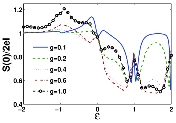
Figure 2: (Color online) Fano factor ${S(0)}/({2eI})$ versus DQD energy gap $\epsilon$ with various $g$. The other parameters are given as $\Delta=0.1$, $\Gamma_{L}=0.1$, $\Gamma_{R}=0.001$ and $\gamma_{b}=0.01$. $\omega_{b}=1$ is set as the energy unit.

3 Results and discussions

In Fig. 2, we first show Fano factor (see Eq. (9)) as comparisons with previous results given in Ref. Lambert1 to validate our method. When the DQD-resonator coupling is weak $(g=0.1,0.2,0.4)$, we find the results obtained by our method are the same as those in Ref. Lambert1 . Moreover, our method with coherent phonon states can also work at strong e-ph coupling regime $(g=1.0)$, where the previous method with Fock states fails.

In the following, with the help of coherent phonon states, we are capable to scrutinize the DQD’s transport properties mediated by e-ph coupling in a full range of strengths. We focus on analyzing the first three cumulants of probability distribution of electron current, though higher order cumulants are also available.

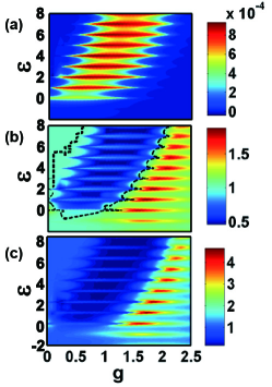
Figure 3: (Color online) Current ($\mathcal{I}^{(1)}$), Fano factor (${\mathcal{I}^{(2)}}/{\mathcal{I}^{(1)}}$) and RTOC (${\mathcal{I}^{(3)}}/{\mathcal{I}^{(1)}}$) are numerically calculated in (a), (b) and (c) under parameters of $g$ and $\varepsilon$. Dashed black line in (b) is used to signify Poissonion transport with Fano factor equal to $1$. The other parameters are given as $\Delta=0.1$, $\Gamma_{L}=0.1$, $\Gamma_{R}=0.001$, $\gamma_{b}=0.01$ and $\omega_{b}=1$.

In Fig. 3(a), by tuning the energy level mismatch $\varepsilon$ and e-ph coupling $g$, we find there exist multiple resonance islands of current, where $\mathcal{I}^{(1)}$ suddenly becomes large under the integer relation $\varepsilon=k\omega_{b}$, $k\in\mathbb{N}$, as is also discovered in Refs. Brandes2 ; Armour . This integer relation indicates that the electron tunneling is strongly assisted by $k$-phonon excitations from the mechanical resonator when the energy gap of two quantum dots is equal to the energy of $k$ phonons. That is, the tunneling from quantum dot $L$ to $R$ will be significantly enhanced if the excess energy can excite integer number of phonons of the resonator’s vibration, which are then absorbed by the zero temperature thermal environment.

The positive integer resonance is, however, not always satisfied in regimes of large energy mismatch of DQD $(\varepsilon\gg{\omega_{b}})$ and weak e-ph coupling $(g\ll{\omega_{b}})$ where it is insufficient to excite extra phonons, or in regimes of extremely strong coupling $(g\gg{\omega_{b}})$ where e-ph coupling plays the role of scattering and strongly represses the electron current. For negative $\epsilon$, the current is drastically suppressed by the fact that the resonator has the ability only to emit phonons to the thermal environment of zero temperature. If we increase the temperature of the environment, the resonance peak emerging at negative integer values of $\epsilon$ will be observed. We note that in a different setup of triple quantum dots Dominguez , similar integer relation for current is exhibited, but as dips (repressions) rather than peaks (enhancements).

Fano factor shown in Fig. 3(b), is more complicated than the current. We separate the plot into two sub-regimes by the dashed black line, which notifies Poissonion transport. In the regime surrounded by this line, Fano factor drops into sub-Poisson regime, where the coupling strength $g$ is moderate Lambert1 . The shrink of Fano factor mainly results from the dramatic increasing of current induced by e-ph excitations. When $g$ becomes strong, Fano factor rises to super-Poisson regime due to the repression of currents. Furthermore, resonance enhancements of Fano factor at integer $\varepsilon$ are clearly observed in both regimes of positive and negative $\varepsilon$ with strong $g$.

Fig. 3(c) shows the renormalized third order cumulant (RTOC), which should not be ignored to signify high order transport fluctuations Flindt ; Flindt2 . For moderate $g$, RTOC is rather small due to resonances of the current. While $g$ reaches strong regime, RTOC is strengthened, mainly due to the repression of currents shown in Fig. 3(a). The multi-phonon-resonance-induced RTOC enhancement still appears, which is similar to what happens for shot noise.

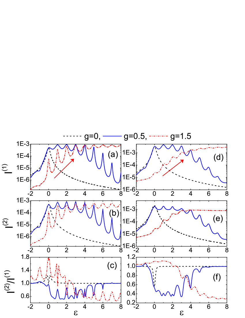
Figure 4: (Color online) Current $\mathcal{I}^{(1)}$, shot noise $\mathcal{I}^{(2)}$ and Fano factor $\mathcal{I}^{(2)}/\mathcal{I}^{(1)}$ as a function of $\varepsilon$ for different $g$. Asymmetric tunneling rates condition: $\Delta=0.1$, $\Gamma_{L}=0.1$, $\Gamma_{R}=0.001$ and $\gamma_{b}=0.01$ for (a), (b) and (c); Symmetric tunneling rates condition: $\Delta=0.1$, $\Gamma_{L}=0.01$, $\Gamma_{R}=0.01$ and $\gamma_{b}=0.05$ for (d), (e) and (f).

To understand the complicated behaviors of Fano factor, we detail the dependence of current fluctuations on DQD energy gap $\varepsilon$ in Fig. 4. Peaks appear at $\varepsilon=k\omega_{b}$ for both current and shot noise, resulting from the integer phonon resonance. When $g$ is moderate (exemplified by $g=0.5$), oscillatory decays of both current and shot noise in Fig. 4(a)(b) and (d)(e) are visible for $\varepsilon>4.0$ while Fano factor rises gradually from sub-Poisson regime to $1.0$ with oscillations, see Fig. 4(c)(f). This can be interpreted that for large $\varepsilon$ compared to $g$, the e-ph coupling is not able to assist the electron transport and tunneling events between quantum dots are seldom, so that successive transmissions of electrons are almost uncorrelated. As a result, the transport dynamics approaches Poissonion regime such that $S(0)\approx 2eI$. When $g$ is strong (exemplified by $g=1.5$), current and shot noise are lifted as $\varepsilon$ increases (see Fig. 4(a)(b)), indicated by the arrows. It suggests that multi-phonon excitations are definitely favored in large e-ph coupling $g$ regime to enhance both the current and shot noise. Though not depicted here, we still observe that current and corresponding shot noise will reach the maximum and then decreases when we increase $\varepsilon$ to extremely large values.

Although the phonon-assisted tunneling that is excited by e-ph coupling is not expected at the negative integer value of $\varepsilon$ at zero temperature, the resonance peaks are still observed in Fig. 4(c)(f) for Fano factor. These peaks result from the dips of current at the negative integer $\varepsilon$, shown in Fig. 4(a)(d). The dips are due to the interference between the elastic and inelastic transmission scattered by the e-ph coupling, instead of opening new tunneling channels by e-ph coupling Galperin .

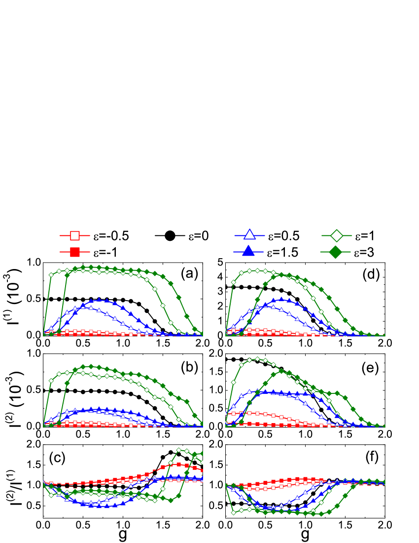
Figure 5: (Color online) Current $\mathcal{I}^{(1)}$, shot noise $\mathcal{I}^{(2)}$ and Fano factor $\mathcal{I}^{(2)}/\mathcal{I}^{(1)}$ as a function of $g$ for some representative $\varepsilon$. Asymmetric tunneling rates condition: $\Delta=0.1$, $\Gamma_{L}=0.1$, $\Gamma_{R}=0.001$ and $\gamma_{b}=0.01$ for (a), (b) and (c); Symmetric tunneling rates condition: $\Delta=0.1$, $\Gamma_{L}=0.01$, $\Gamma_{R}=0.01$ and $\gamma_{b}=0.05$ for (d), (e) and (f).

The dependencies of current, shot noise and Fano factor on $g$ are detailed in Fig. 5, with four typical transport behaviors exemplified therein:

(1) The first kind behavior appears at $\varepsilon<0$ (exemplified by $\varepsilon=-0.5,-1$), where current and shot noise are both rather small in the whole regime of $g$. This is understandable since in this regime electrons in DQD are severely localized, and there is no feedback of phonons from noise environment with zero temperature. As a result, electrons cannot effectively transfer through DQD by phonon-assisted tunneling.

(2) $\varepsilon=0$ depicts the second kind behavior. When $g\lesssim 1.0$, current, shot noise and Fano factor are only slightly affected, which show that for the DQD with two degenerate energy levels, the transport properties are robust for weak e-ph couplings. When $g$ increases further, the scattering effect of e-ph coupling becomes significant and the current decreases. In the absence of e-ph coupling and $\varepsilon=0$, the current can be described Nazarov1 by

$$\mathcal{I}^{(1)}=\frac{{\Delta}^{2}\Gamma_{R}}{\Delta^{2}(2+\Gamma_{R}/\Gamma_{L})+\Gamma_{R}^{2}/4+\varepsilon^{2}}.$$ (19)

Consequently, for the case of asymmetric tunneling rates, $\mathcal{I}^{(1)}\approx{\Gamma_{R}}/{2}=0.0005$, while for the symmetric tunneling case $\mathcal{I}^{(1)}\approx{\Gamma_{R}}/{3}=0.0033$, consistent with what are shown in Fig. 5(a) and (d). In Refs. Elattari ; Brandes3 , the exact result of Fano factor is obtained without considering e-ph coupling ($g=0$):

$$1-8{\Delta^{2}}\frac{4\varepsilon^{2}(\Gamma_{R}/\Gamma_{L}-1)+3\Gamma_{R}^{2}+\Gamma_{R}^{3}/\Gamma_{L}+8\Gamma_{R}/\Gamma_{L}\Delta^{2}}{[\Gamma_{R}^{2}+4\varepsilon^{2}+4\Delta^{2}(\Gamma_{L}/\Gamma_{R}+2)]^{2}}.$$ (20)

For $\varepsilon=0$, we then can approximately simplify Fano factor as $1$ for asymmetric tunneling case $\Gamma_{R}\ll\Gamma_{L}$ and as $\frac{5}{9}$ for symmetric tunneling case $\Delta\gg\Gamma_{R}=\Gamma_{L}$. These coincide with the simulation results shown in Fig. 5(c) and (f), where Fano factor is nearly $1.0$ for the asymmetric case, indicating the Poissonion nature while it is strongly suppressed around $0.5$ when $g\lesssim 1.0$ for the symmetric tunneling.

(3) The third kind behavior is for positive but non-integer $\varepsilon$ (exemplified by $\varepsilon=0.5,1.5$). As shown in Fig. 5(a) and (d), these two curves of currents first increase when $g$ increases as a consequence of phonon-assisted tunneling. An then, when the e-ph coupling strength $g$ is further increased, the currents decrease because of the phonon-scattering-induced localization. In Fig. 5(b)(e), shot noise changes almost synchronously with currents, however, with smaller amplitude variations compared to currents. Hence, Fano factor experiences from sub-Poisson to Poisson regime, gaining a global minimum around $0.5$.

(4) Positive integer $\varepsilon$ (exemplified by $\varepsilon=1,3$) depicts the forth kind behavior, that is, the resonant electron tunneling regime. The e-ph coupling first plays a constructive role to assist electron tunneling. While, as the coupling strength $g$ increases, the resonator’s vibration scatters electrons and suppresses the current dramatically. This is similar to the non-integer $\varepsilon$ cases and the difference is that the maximum of the resonant cases is more like a platform. Generally, near the resonances, one can write Haugbook :

$$\mathcal{I}^{(1)}=\int\frac{d\varepsilon}{2\pi}\frac{\Gamma_{L}\Gamma_{R}}{(\varepsilon-k\omega_{b})^{2}+(\Gamma_{L}+\Gamma_{R})^{2}/4}[f_{L}-f_{R}].$$ (21)

This can be successively approximated as $\mathcal{I}^{(1)}\approx\frac{\Gamma_{L}\Gamma_{R}}{\Gamma_{L}+\Gamma_{R}}$ in the weak $\Gamma_{L(R)}$ limit, since the Lorentz function reduces to the delta function. Therefore, for asymmetric tunneling case $\Gamma_{R}\ll\Gamma_{L}$, the resonant current nearly reaches the maximum $\mathcal{I}^{(1)}=\Gamma_{R}$ and for symmetric tunneling case $\Gamma_{R}=\Gamma_{L}$, the resonant current nearly reaches the maximum $\mathcal{I}^{(1)}={\Gamma_{R}}/{2}$, which are consistent with our calculations shown in Fig. 5(a) and (d). Furthermore, different from the non-integer $\varepsilon$ cases, for integer $\varepsilon$ Fano factor exhibits two local minimums at its minimum basin in the sub-Poisson regime, as shown in Fig. 5(c) and (f).

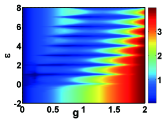
Figure 6: (Color online) ${\langle}\sigma_{z}(a^{\dagger}+a){\rangle}$ as a function of $g$ and $\varepsilon$. Other parameters are $\Delta=0.1$, $\Gamma_{L}=0.1$, $\Gamma_{R}=0.001$, $\gamma_{b}=0.01$.

In Fig. 6, we show the expectation of the e-ph interaction term, ${\langle}\sigma_{z}(a^{\dagger}+a){\rangle}$, to exam the role of e-ph interaction in the transport. ${\langle}\sigma_{z}(a^{\dagger}+a){\rangle}=\langle|L{\rangle}{\langle}L|(a^{{\dagger}}+a){\rangle}-\langle|R{\rangle}{\langle}R|(a^{{\dagger}}+a){\rangle}$ describes the discrepancy of resonator displacement’s contributions on electron occupancies on the left and right quantum dots. Under resonance conditions $(\varepsilon=k\omega_{b})$, the discrepancy ${\langle}\sigma_{z}(a^{\dagger}+a){\rangle}$ is rather small, compared to off-resonance cases with the same $g$, which indicates the electron occupation probabilities on the two quantum dots are almost equivalent. That is, the phonon emission of the resonator into the thermal environment assists electron transferring from the left quantum dot to the right one, rather than blocks electron transport. This is consistent with multi-phonon-assisted resonance discussed in Fig. 3 and 4.

However, when the e-ph coupling $g$ becomes strong, the discrepancy ${\langle}\sigma_{z}(a^{\dagger}+a){\rangle}$ becomes significant for given $\varepsilon$, which implies the phonon assistance mechanism is depressed. The e-ph interaction no longer assists electron tunneling, but plays the role of scattering. Hence, the electron is mainly localized in the left quantum dot (indicated by the significantly positive value of ${\langle}\sigma_{z}(a^{\dagger}+a){\rangle}$) due to the e-ph scattering, which results in the repression of the electron current, as shown in Figs. 3 and 5.

4 Summary

To conclude, we have applied the modified Born-Markov quantum master equation to investigate full counting statistics of electron transport through the double quantum dots coupled with a nanomechanical resonator. Particularly, with the help of coherent phonon states method, we are capable to non-perturbatively treat the e-ph coupling of arbitrary strong strength, with excellent convergence. We have shown the first three order current fluctuations in detail to signify the non-Poissonion electron transport features in different dynamics regimes. Conditional phonon-assisted resonant tunneling has been observed under the positive integer relation of $\varepsilon=k\omega_{b},k\in\mathbb{N}$. We have further found that, in strong e-ph coupling regime, multi-phonon excitations are favored such that transport is enhanced with increasing energy gap $\varepsilon$. Moreover, for positive $\varepsilon$, we have found that as the strength $g$ increases, the e-ph coupling first plays a constructive role to assist the transport, and then plays the role of scattering and strongly represses the transport. Finally, we have studied the expectation value of DQD-resonator interaction to show the difference of contributions between quantum dots, which complements out understanding on multi-phonon-assisted electron tunneling and phonon-scattering-induced electron localization in strong e-ph regimes.

Though not fully exploited yet, the extended coherent phonon states method may be extended to directly investigate dissipative DQD system with multiple-phonon-electron coupling Chen2 . We expect our method can be applied to other open quantum systems beyond weak e-ph interaction constraints, to uncover possible novel many-body quantum effects induced by strong e-ph interactions, like the avalanche type of transport Koch .

5 Acknowledgements

We thank Dr. Y. Y. Zhang for helpful discussions. This work (C.W. and Q.H.C.) is supported in part by National Natural Science Foundation of China under Grant No. 10974180, National Basic Research Program of China under Grant Nos. 2011CBA00103 and 2009CB929104.

Appendix A Derivation of Quantum Master Equation under Counting Field

The whole Hamiltonian including system and environments under counting field can be described by $H_{\chi}=H_{0}+V_{\chi}$ given in Eq. (3). Here $H_{0}=H_{S}+H_{\textrm{Lead}}+H_{E}$ shows noninteracting term and $V_{\chi}=V_{\textrm{RE}}+V_{\textrm{DL}}(\chi)$ is treated as perturbation one, assuming the interacting between system and environment/electrodes is weak (not the e-ph coupling inside the system).

Under interacting picture, the motion equation of density matrix from the whole model can be shown as

$$~{}\frac{d{\rho^{I}_{\chi}(t)}}{d{t}}=-i[V_{\chi}(t),\rho^{I}_{\chi}(t)],$$ (22)

where $\rho^{I}_{\chi}(t)=e^{iH_{0}t}\rho_{\chi}(t)e^{-iH_{0}t}$ and $V_{\chi}(t)=e^{iH_{0}t}V_{\chi}e^{-iH_{0}t}$. By integrating Eq. (22), density matrix can be expressed as

$${\rho^{I}_{\chi}(t)} = \rho_{\chi}(0)-i\int^{t}_{0}dt^{\prime}[V_{\chi}(t^{\prime}),{\rho^{I}_{\chi}(t^{\prime})}],$$

$$= \rho_{\chi}(0)-i\int^{t}_{0}dt^{\prime}[V_{\chi}(t^{\prime}),{\rho_{\chi}(0)}]$$

$$-\int^{t}_{0}dt^{\prime}\int^{t^{\prime}}_{0}d{\tau}[V_{\chi}(t^{\prime}),[V_{\chi}(\tau),\rho^{I}_{\chi}(\tau)]].$$

Hence the density matrix motion equation in interacting picture can be derived by

$$~{}\frac{d{\rho^{I}_{\chi}(t)}}{dt} = -i[V_{\chi}(t),\rho_{\chi}(0)]$$

$$-\int^{t}_{0}d{\tau}[V_{\chi}(t),[V_{\chi}(\tau),\rho^{I}_{\chi}(\tau)]],$$

Transforming it back to the Schrödinger picture, one can find the reduced system density matrix can be expressed by $\rho^{S}_{\chi}(t)=\textrm{Tr}_{\textrm{{E,Lead}}}[e^{-iH_{0}t}\rho^{I}_{\chi}(t)e^{iH_{0}t}].$ As a result, the motion equation of the reduced system density matrix is shown by

$$\frac{d\rho^{S}_{\chi}(t)}{dt} = -i[H_{S},\rho^{S}_{\chi}(t)]$$

$$-\int^{\infty}_{0}d\tau{\langle}[V_{\chi},[V_{\chi}(-\tau),\rho_{\chi}(t)]_{\chi}]_{\chi}{\rangle}_{\textrm{E,Lead}}.$$

Here Born approximation is applied to decompose the whole density matrix as $\rho_{\chi}(t)=\rho^{S}_{\chi}(t)\otimes{\rho_{E}}\otimes{\rho_{{Lead}}}$. Markov approximation should be also considered to replace $\rho^{I}_{\chi}(\tau)$ in the right second term of Eq. (A) by $\rho^{I}_{\chi}(t)$ and extend the upper integral limit from $t$ to $\infty$. Besides, $[A_{\chi},B_{\chi}]_{\chi}=A_{\chi}B_{\chi}-B_{\chi}A_{-\chi}$ and ${\langle}O{\rangle}_{\textrm{E,Lead}}$ shows statistical average of $O$ over thermal environment and leads.

Appendix B Derivation of Density Matrix Equation

The evolution Eq. (18) has five blocks specified by the five electron states. Let us denote the reduced system density matrix elements combined with counting field as

$$\rho^{ji}_{n,m}={{}_{j}{\langle}}n|{\langle}j|\rho^{S}_{\chi}|i{\rangle}|m{\rangle}_{i}.$$

Then the first block describes the evolution of elements in ${\rho_{00}}$:

$$\frac{d}{dt}\rho^{00}_{n,m}=-i\omega_{b}(n-m)\rho^{00}_{n,m}-{\Gamma_{L}}\rho^{00}_{n,m}$$

$$+\Gamma_{R}\sum_{k,l}{{}_{0}\langle}n|k{\rangle_{R}}{{}_{R}\langle}l|m{\rangle_{0}}e^{i\chi}\rho^{RR}_{k,l}$$

$$-\frac{\gamma_{b}}{2}[(n+m)\rho^{00}_{n,m}-2\sqrt{(n+1)(m+1)}\rho^{00}_{n+1,m+1}]$$

$$+\bar{n}\gamma_{b}[-(n+m)\rho^{00}_{n,m}+\sqrt{(n+1)(m+1)}\rho^{00}_{n+1,m+1}$$

$$+\sqrt{nm}\rho^{00}_{n-1,m-1}].$$

The second block is for the evolution of ${\rho_{LL}}$:

$$\frac{d}{dt}\rho^{LL}_{n,m}=-i\omega_{b}(n-m)\rho^{LL}_{n,m}+{\Gamma_{L}}\sum_{k,l}{{}_{L}\langle}n|k{\rangle_{0}}{{}_{0}\langle}l|m{\rangle_{L}}\rho^{00}_{k,l}$$

$$-i\Delta\sum_{k}{{}_{L}\langle}n|k{\rangle_{R}}\rho^{RL}_{k,m}+i\Delta\sum_{k}\rho^{LR}_{n,k}{{}_{R}\langle}k|m{\rangle_{L}}$$

$$-\frac{\gamma_{b}}{2}[(n+m)\rho^{LL}_{n,m}-\alpha\sqrt{n}\rho^{LL}_{n-1,m}$$

$$+\alpha\sqrt{n+1}\rho^{LL}_{n+1,m}+\alpha\sqrt{m+1}\rho^{LL}_{n,m+1}$$

$$-\alpha\sqrt{m}\rho^{LL}_{n,m-1}-2\sqrt{(n+1)(m+1)}\rho^{LL}_{n+1,m+1}]$$

$$+\bar{n}\gamma_{b}[-(n+m)\rho^{LL}_{n,m}+\sqrt{(n+1)(m+1)}\rho^{LL}_{n+1,m+1}$$

$$+\sqrt{nm}\rho^{LL}_{n-1,m-1}].$$

The third block is for the evolution of ${\rho_{RR}}$:

$$\frac{d}{dt}\rho^{RR}_{n,m}=-i\omega_{b}(n-m)\rho^{RR}_{n,m}-\Gamma_{R}\rho^{RR}_{n,m}$$

$$+i\Delta\sum_{k}{{}_{L}\langle}k|m{\rangle_{R}}\rho^{RL}_{n,k}-i\Delta\sum_{k}{{}_{R}\langle}n|k{\rangle_{L}}\rho^{LR}_{k,m}$$

$$-\frac{\gamma_{b}}{2}[(n+m)\rho^{RR}_{n,m}+\alpha\sqrt{n}\rho^{RR}_{n-1,m}$$

$$-\alpha\sqrt{n+1}\rho^{RR}_{n+1,m}-\alpha\sqrt{m+1}\rho^{RR}_{n,m+1}$$

$$+\alpha\sqrt{m}\rho^{RR}_{n,m-1}-2\sqrt{(n+1)(m+1)}\rho^{RR}_{n+1,m+1}].$$

The fourth block is for the evolution of ${\rho_{RL}}$:

$$\frac{d}{dt}\rho^{RL}_{n,m}=i[\varepsilon\rho^{RL}_{n,m}+\Delta\sum_{k}{{}_{R}\langle}k|m{\rangle_{L}}\rho^{RR}_{n,k}$$

$$-\Delta\sum_{k}{{}_{R}\langle}n|k{\rangle_{L}}\rho^{LL}_{k,m}+\omega_{b}(m-n)\rho^{RL}_{n,m}]$$

$$-\frac{\Gamma_{R}}{2}\rho^{RL}_{n,m}-\frac{\gamma_{b}}{2}[(n+m+4\alpha^{2})\rho^{RL}_{n,m}$$

$$+3\alpha\sqrt{n+1}\rho^{RL}_{n+1,m}-\alpha\sqrt{n}\rho^{RL}_{n-1,m}$$

$$-3\alpha\sqrt{m+1}\rho^{RL}_{n,m+1}-\alpha\sqrt{m}\rho^{RL}_{n,m-1}$$

$$-2\sqrt{(n+1)(m+1)}\rho^{RL}_{n+1,m+1}]$$

$$+\bar{n}\gamma_{b}[-(n+m+4\alpha^{2})\rho^{RL}_{n,m}$$

$$-2\alpha(\sqrt{n+1}\rho^{RL}_{n+1,m}+\sqrt{n}\rho^{RL}_{n,m})$$

$$+2\alpha(\sqrt{m+1}\rho^{RL}_{n,m+1}+\sqrt{m}\rho^{RL}_{n,m-1})$$

$$+\sqrt{(n+1)(m+1)}\rho^{RL}_{n+1,m+1}+\sqrt{nm}\rho^{RL}_{n-1,m-1}].$$

So is the last block for ${\rho_{LR}}$:

$$\frac{d}{dt}\rho^{LR}_{n,m}=-i[\varepsilon\rho^{LR}_{n,m}+\Delta\sum_{k}{{}_{L}\langle}n|k{\rangle_{R}}\rho^{RR}_{k,m}$$

$$-\Delta\sum_{k}{{}_{L}\langle}k|m{\rangle_{R}}\rho^{LL}_{n,k}+\omega_{b}(n-m)\rho^{LR}_{n,m}]$$

$$-\frac{\Gamma_{R}}{2}\rho^{LR}_{n,m}-\frac{\gamma_{b}}{2}[(n+m+4\alpha^{2})\rho^{LR}_{n,m}$$

$$-3\alpha\sqrt{n+1}\rho^{LR}_{n+1,m}-\alpha\sqrt{n}\rho^{LR}_{n-1,m}$$

$$+3\alpha\sqrt{m+1}\rho^{LR}_{n,m+1}+\alpha\sqrt{m}\rho^{LR}_{n,m-1}$$

$$-2\sqrt{(n+1)(m+1)}\rho^{LR}_{n+1,m+1}]$$

$$+\bar{n}\gamma_{b}[-(n+m+4\alpha^{2})\rho^{LR}_{n,m}$$

$$+2\alpha(\sqrt{n+1}\rho^{LR}_{n+1,m}+\sqrt{n}\rho^{LR}_{n-1,m})$$

$$-2\alpha(\sqrt{m+1}\rho^{LR}_{n,m+1}+\sqrt{m}\rho^{LR}_{n,m-1})$$

$$+\sqrt{(n+1)(m+1)}\rho^{LR}_{n+1,m+1}+\sqrt{nm}\rho^{LR}_{n-1,m-1}].$$

For the inner-product of the coherent phonon states in these evolution equations, the expression can be deduced by following Eq. (14) to (16):

$${}_{L}{\langle}n|m\rangle_{0} = {}_{0}{\langle}n|m\rangle_{R}=(-1)^{m}D_{nm}(\alpha),$$

$${}_{L}{\langle}n|m\rangle_{R} = (-1)^{m}D_{nm}(2\alpha),$$

$${}_{R}{\langle}n|m\rangle_{L} = (-1)^{m}D_{nm}(-2\alpha),$$

$$\text{with}\quad D_{nm}(x) = \sqrt{n!m!}\exp{(-\frac{x^{2}}{2})}x^{n+m}$$

$$\times\sum_{k=0}^{\min\{n,m\}}\frac{x^{-2k}(-1)^{k}}{(n-k)!(m-k)!k!}.$$

In the practical calculations, the truncation number of phonon occupation states is set as Ntr. Given a specified Ntr, there exist $5(\textrm{Ntr}+1)^{2}$ equations in all, where the $5$ characterizes the space dimension of electron states. Thanks to the overcomplete property of coherent phonon states, the truncation number of modified phonon space has much shrinked even when $g$ becomes large. Through our whole work, we set $\textrm{Ntr}\leq 30$. We have checked that this number is enough and all the results converge with relative errors less than $10^{-5}$.

References

- (1) T. A. Fulton and G. J. Dolan, Phys. Rev. Lett. 59, 109 (1987); H. Grabert and M. H. Devoret, Single Charge Tunneling (Plenum, New York, 1992).
- (2) R. Ashoori, Nature (London) 379, 413 (1996).
- (3) C. Joachim, J. K. Gimzewski, and A. Aviram, Nature (London) 408, 541 (2000); H. Park, J. Park, A. K. L. Lim, E. H. Anderson, A. P. Alivisatos, and P. L. McEuen, Nature (London) 407, 57 (2000).
- (4) A. Aviram and M. A. Ratner, Chem. Phys. Lett. 29, 277 (1974).
- (5) C. Joachim, J. K. Gimzewski, R. R. Schlittler, and C. Chavy, Phys. Rev. Lett. 74, 2102 (1995).
- (6) L. A. Bumm et al., Science 271, 1705 (1996).
- (7) M. A. Reed, C. Zhou, C. J. Muller, P. Burgin, and J. M. Tour, Science 278, 252 (1997).
- (8) H. G. Craighead, Science 290, 1532 (2000).
- (9) A. N. Cleland, Foundations of Nanomechanics (Springer, Berlin, 2003).
- (10) M. Blencowe, Phys. Rep. 395, 159 (2004).
- (11) W. G. van der Wiel, S. D. Franceschi, J. M. Elzerman, T. Fujisawa, S. Tarucha, and L. P. Kouwenhowen, Rev. Mod. Phys. 75, 1 (2003).
- (12) Y. Nakamura et al., Nature (London) 398, 786 (1999).
- (13) D. Vion et al., Science 296, 886 (2002).
- (14) I. Chiorescu et al., Science 299, 1869 (2003).
- (15) Y. A. Pashkin et al., Nature (London), 421, 823 (2003).
- (16) T. Fujisawa et al., Science, 282, 932 (1998).
- (17) T. Brandes and B. Kramer, Phys. Rev. Lett. 83, 3021 (1999).
- (18) R. S. Knobel and A. N. Cleland, Nature (London) 424, 291 (2003).
- (19) M. D. LaHaye et al., Science 304, 74 (2004).
- (20) A. Naik et al., Nature (London) 443, 193 (2006).
- (21) A. A. Clerk and S. Bennett, New J. Phys. 7, 238 (2005).
- (22) G. Kießlich, E. Schöll, T. Brandes, F. Hohls, and R. J. Haug, Phys. Rev. Lett. 99, 206602 (2007).
- (23) R. Sánchez, S. Kohler, P. Hänggi, and G. Platero, Phys. Rev. B 77, 035409 (2008)
- (24) Y. M. Blanter and M. Büttiker, Phys. Rep. 336, 1 (2000).
- (25) Quantum Noise in Mesoscopic Physics, edited by Y. V. Nazarov (Kluwer, Dordrecht, 2003).
- (26) L. S. Levitov and G. B. Lesovik, JETP Lett. 58, 230 (1993); L. S. Levitov, H. Lee, and G. B. Lesovik, J. Math. Phys. 37, 4845 (1996).
- (27) H. B. Sun and G. J. Milburn, Phys. Rev. B. 59, 10748 (1999).
- (28) D. A. Bagrets and Y. V. Nazarov, Phys. Rev. B 67, 085316 (2003).
- (29) R. Aguado and T. Brandes, Phys. Rev. Lett. 92, 206601 (2004).
- (30) D. A. Bagrets and Y. V. Nazarov, Phys. Rev. Lett. 94, 056801 (2005).
- (31) J. Ren, P. Hänggi, and B. Li, Phys. Rev. Lett. 104, 170601 (2010).
- (32) L. Wei, J. ZhingQing, L. Pfeiffer, K. W. West, and A. J. Rimberg, Nature (London) 423, 422 (2003).
- (33) J. Bylander, T. Duty, and P. Delsing, Nature (London) 434, 361 (2005).
- (34) S. Gustavsson, R. Leturcq, B. Simovič, R. Schleser, T. Ihn, P. Studerus, K. Ensslin, D. C. Driscoll, and A. C. Gossard, Phys. Rev. Lett. 96, 076605 (2006).
- (35) M. Campisi, P. Hänggi, and P. Talkner, Rev. Mod. Phys. 83, 771 (2011).
- (36) C. Flindt, T. Novotný, A. Braggio, M. Sassetti, and A.-P. Jauho, Phys. Rev. Lett. 100, 150601 (2008).
- (37) C. Flindt, T. Novotný, and A.-P. Jauho, Europhys. Lett. 69, 475 (2005).
- (38) S. R. S. Varadhan, Comm. Pure Appl. Math. 19, 261 (1966).
- (39) A. Dembo and O. Zeitouni, Large Deviations: Techniques and Applications, 2nd ed. (Springer, 1998).
- (40) H. Touchette, Phys. Rep. 478, 1 (2009).
- (41) E. K. Irish, Phys. Rev. Lett. 99, 173601 (2007).
- (42) M. J. Hwang and M. S. Choi, Phys. Rev. A 82, 025802 (2010).
- (43) Q. H. Chen, Y. Y. Zhang, T. Liu, and K. L. Wang, Phys. Rev. A 78, 051801 (2008); Q. H. Chen, T. Liu, Y. Y. Zhang, and K. L. Wang, Phys. Rev. A 82, 053841 (2010).
- (44) Y. Y. Zhang, Q. H. Chen, and K. L. Wang, Phys. Rev. B 81, 121105 (2010).
- (45) N. Lambert and F. Nori, Phys. Rev. B 78, 214302 (2008).
- (46) H. Park, J. Park, A. K. L. Lim, E. H. Anderson, A. P.Alivisatos, and P. L. McEuen, Nature (London) 407, 57 (2000).
- (47) B. J. LeRoy, S. G. Lemay, J. Kong, and C. Dekker, Nature (London) 432, 371 (2004).
- (48) S. Sapmaz, P. Jarillo-Herrero, Ya. M. Blanter, C. Dekker, and H. S. J. van der Zant, Phys. Rev. Lett. 96, 026801 (2006).
- (49) T. Niemczyk, F. Deppe, H. Huebl, E. P. Menzel, F. Hocke, M. J. Schwarz, J. J. Garcia-Ripoll, D. Zueco, T. Hümmer, E. Solano, A. Marx, and R. Gross, Nature (London) 6, 772 (2010).
- (50) M. Esposito, U. Harbola and S. Mukamel, Rev. Mod. Phys. 81, 1665 (2009).
- (51) T. Brandes and N. Lambert, Phys. Rev. B 67, 125323 (2003).
- (52) G. D. Mahan, Many-Particle Physics (New York, 1990).
- (53) A. D. Armour and A. MacKinnon, Phys. Rev. B 66, 035333 (2002).
- (54) F. Domínguez, S. Kohler, and G. Platero, Phys. Rev. B 83, 235319 (2011).
- (55) M. Galperin, M. A. Ratner, A. Nitzan, and A. Troisi, Science 319, 1056 (2008).
- (56) T. H. Stoof and Y. V. Nazarov, Phys. Rev. B 53, 1050 (1996).
- (57) B. Elattari and S. A. Gurvitz, Phys. Lett. A 292, 289 (2002).
- (58) T. Brandes, Phys. Rep. 408, 315 (2005).
- (59) H. Haug and A. P. Jauho, Quantum Kinetics in Transport and Optics of Semiconductors (Springer-Verlag, Berlin, 2008).
- (60) J. Koch and F. von Oppen, Phys. Rev. Lett. 94, 206804 (2005).