Calibrating Emission Lines as Quasar Bolometers

Abstract

Historically, emission lines have been considered a valuable tool for estimating the bolometric thermal luminosity of the accretion flow in AGN, $L_{bol}$. We study the reliability of this method by comparing line strengths to the optical/UV continuum luminosity of SDSS DR7 radio quiet quasars with $0.4<z<0.8$. We find formulae for $L_{bol}$ as a function of single line strengths for the broad components of H$\beta$ and Mg II, as well as the narrow lines of [O III] and [O II]. We determine the standard errors of the formulae that are fitted to the data. Our new estimators are shown to be more accurate than archival line strength estimations in the literature. It is demonstrated that the broad lines are superior estimators of the continuum luminosity (and $L_{bol}$) with $H\beta$ being the most reliable. The fidelity of the each of the estimators is determined in the context of the SDSS DR7 radio loud quasars as an illustrative application of our results. In general, individual researchers can use our results as a tool to help decide if a particular line strength provides an adequate estimate of $L_{bol}$ for their purposes. Finally, it is shown that considering all four line strength, simultaneously, can yield information on both $L_{bol}$ and the radio jet power.

The primary measure of the strength of an active galactic nucleus (AGN) is its bolometric luminosity, $L_{bol}$, the broadband thermal luminosity from IR to X-ray. The characteristic signature of the thermal component is the ”big blue bump” a large blue/UV excess in the spectral continuum (Sun and Malkan, 1989). Typically, one does not have complete frequency coverage of the broadband continuum and $L_{bol}$ can only be estimated. The most common estimators involve single point rest frame optical or UV luminosity as an approximation to the big blue bump, Kaspi et al (2000), or the luminosity of the optical continuum as in Miller et al (1992). However, there are many instances in which the optical/UV continuum is not directly observable or is contaminated with other sources of flux. Thus, astrophysicists need a surrogate for the continuum luminosity. The two most prevalent situations that are encountered are firstly, blazars in which the synchrotron optical/UV emission from the relativistic jet is Doppler boosted to a brightness that either swamps the quasar thermal emission or contributes an unknown fraction of the total observed optical/UV flux. The other common occurrence is when dusty molecular gas (e.g., the ”dusty torus”) obscures the thermal emission produced by the quasar accretion flow from our view. The latter case is believed to be representative of NLRGs (narrow line radio galaxies) and Seyfert 2 galaxies (Antonucci, 1993). Historically, broad line strengths have been used as a surrogate for continuum luminosity in blazars (Cao and Jiang, 2001; Celotti and Fabian, 1993; Celotti et al, 1997; Ghisellini et al, 2011; Gu et al, 2009; Maraschi and Tavecchio, 2003; Wang et al, 2004). For NLRGs, the broad line region is not visible by definition and narrow emission line strengths have been used as a surrogate for the continuum luminosity (Rawlings and Saunders, 1991; Willott et al, 1999).

These relationships between line strength and $L_{bol}$ have never been carefully calibrated or scrutinized for their accuracy. This Letter intends to do both with a carefully selected, large sample of SDSS DR7 radio quiet quasars ($0.4<z<0.8$) in which two prominent narrow lines ([OIII] $\lambda$5007 and [OII] $\lambda$3727) and two broad lines H$\beta$ $\lambda$4861 and Mg II $\lambda$2798 are observable for all objects. This allows us to compare the various derived estimators in the context of a single sample of objects, which removes the uncertainties associated with sample selection biases if a different set of objects is used for the calibrations of each individual line strength based estimator. In section 4, we consider these estimators in the context of the radio loud subsample of the SDSS DR7 quasars ($0.4<z<0.8$).

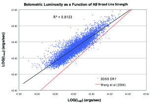
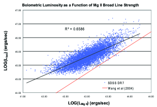
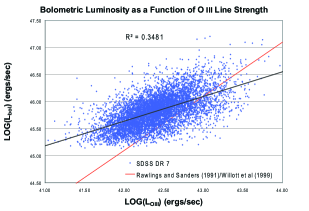
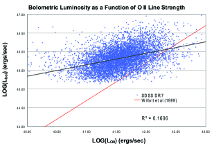
Figure 1: Scatter plots of the logarithm of the line strengths as a function of the logarithm of $L_{\mathrm{bol}}=15L_{\mathrm{cont}}$, where $L_{\mathrm{cont}}$ is the optical/UV continuum luminosity from 5100 $\AA$ to 3000 $\AA$. The fit to the SDSS DR7 data is given by the black line. The accuracy of the linear representation of the data is given by the coefficient of determination, $\mathbf{R}^{2}$, that is displayed on each plot. An archival estimator from the literature is shown as a red line. Notice that the broad component of H$\beta$ is an excellent representation of $L_{\mathrm{cont}}$ at the top left. The next best estimator is based on the broad component of Mg II in upper right hand frame. The [OIII] $\lambda$5007 based estimator is clearly superior to [OII] $\lambda$3727 based estimator in the bottom row.

1 Sample Selection

In order to determine the dependence of line luminosity on the thermal continuum in a quasar, we constructed a sample of SDSS DR7 radio quiet quasars with $0.4<z<0.8$ and spectra with a median S/N $>$ 7, this yielded 10069 AGNs. Long slit spectroscopy of radio loud AGN often show strong regions of narrow line emission on scales as large as $\sim$ 100 kpc that tend to be aligned with the jet direction (Inksip et al, 2002; Best et al, 2000; McCarthy et al, 1995). The magnitude of this contribution to the narrow line luminosity is largely unknown (Willott et al, 1999). Therefore, we segregated out the radio loud quasars because there is a concern that jet propagation can enhance the line strengths. The SDSS DR7 data was cross-referenced to the FIRST data base. The radio loudness, $R$, is usually defined as a 5 GHz flux density 10 times larger than the $4400\AA$ flux density, $R=S_{5\mathrm{GHz}}/S_{4400\AA}<10$ (Kellermann & Pauliny-Toth, 1969). So any FIRST flux density detection or upper limit that implied $R<10$ was considered radio quiet with 1.4 GHz flux density used instead of 5 GHz flux density. We also eliminated the low ionization broad absorption line quasars from our sample since they are known to have anomalously weak [OIII]$\lambda$5007 and [OII]$\lambda$3727 emission lines (Boroson and Green, 1992; Zhang et al, 2010). In the end, there were 6904 radio quiet sources remaining in our sample.

The spectral data of H$\beta$ and Mg II regime were separately reduced using the procedures of Dong et al (2008); Wang et al (2009) which see for further details, and we will only briefly outline it here. To measure the H$\beta$ line and the [OIII]$\lambda$5007 line, a single power-law fit to the optical continuum in the restframe wavelength range $4200-5600\AA$ was obtained taking into account contributions from both broad and narrow Fe II multiplets that were modeled using the I Zw 1 templates provided by Véron-Cetty et al. (2004). The H$\beta$ emission lines are modeled as multiple Gaussians: at most four broad Gaussians and one narrow Gaussian with FWHM $<$ 900 km $s^{-1}$ for H$\beta$, and one or two Gaussians for each [OIII]$\lambda$4959,5007. To measure the Mg II line, we fit the continuum from the several continuum windows in the restframe wavelength range 2200-3500Å, after subtracting the estimated UV FeII contributions by the Fe II template generated by Tsuzuki et al (2006) and the Balmer continuum using the method by Dietrich et al (2002). Each of the two Mg II doublet lines is modeled with one broad five-parameter Gauss-Hermite series component and one single Gaussian narrow component. Furthermore, the broad components of the doublet lines are set to have the same profile. The narrow components are set to FWHM $<$ 900 km $s^{-1}$ and flux $<$ 10% of the total Mg II flux. Finally, we fit the spectrum in the [OII] regime using one Gaussian for [OII] emission and a single power-law for optical continuum in the restframe wavelength range 3600-3800Å. This process resulted in five pieces of relevant information for every quasar:

• The optical/UV continuum luminosity from 5100 $\AA$ to 3000 $\AA$, $L_{\mathrm{cont}}$

• The luminosity of the broad component of H$\beta$ $\lambda$4861, $L_{H\beta}$

• The luminosity of the broad component of Mg II $\lambda$2798, $L_{MgII}$

• The luminosity of the narrow line [OIII] $\lambda$5007, $L_{OIII}$

• The luminosity of the narrow line [OII] $\lambda$3727, $L_{OII}$

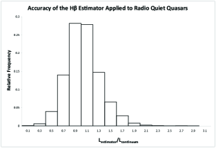
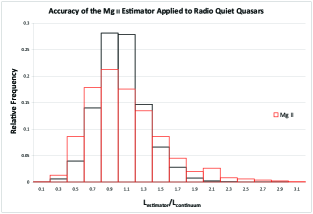
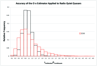
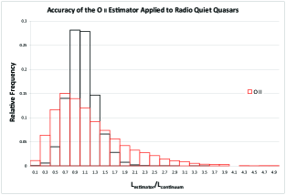
Figure 2: The histograms represent the distributions of the ratio of the estimated continuum flux to the actual continuum flux, $L_{\mathrm{estimated}}/L_{\mathrm{cont}}$ for each of the emission lines in the context of the SDSS DR7 radio quiet subsample. The smallest dispersion about 1 (the most accurate estimator) is H$\beta$ in the upper left hand frame. The superior H$\beta$ fit is shown in black in the other three frames for the sake of comparison.

2 Line Strength Fits to Continuum Luminosity

The blue continuum luminosity is the most basic signature of the thermal emission from the quasar, so it is the most commonly used quantity for estimating $L_{bol}$. Perhaps the most popular bolometric correction is the simple one proposed by Kaspi et al (2000), $L_{bol}\approx 9\lambda L_{\lambda}(5100\,\AA)$. Clearly, using a portion of the optical/UV continuum is more accurate than a single point and we have that at our disposal, $L_{\mathrm{cont}}$. For example, a single point could lie in a noisy end of the SDSS spectrum. The average spectral index in our sample of 6904 quasars, from 5100 $\AA$ to 3000 $\AA$, is $\alpha_{\nu}=0.54$, where $\alpha_{\nu}$ is defined in terms of the spectral luminosity as $L_{\nu}\sim\nu^{-\alpha}$. This spectral slope implies that the Kaspi et al (2000) bolometric correction can be expressed as

$$L_{bol}\approx 15L_{\mathrm{cont}}\;.$$ (1)

Equation (1) is relatively insensitive to the choice of $\alpha$, with only a few percent change in the constant of proportionality as $\alpha$ varies from 0.45 to 0.7.

Figure 1 shows how well the line strengths represent the continuum luminosity with the factor of 15 bolometric correction from equation (1). The linear fits in log-log space are given by equations (2) - (5) with the standard errors for the intercept and the slope

$$\log(L_{bol})=12.32\pm 0.20+(0.78\pm 0.01)\log[L_{H\beta}]\;,$$ (2)

$$\log(L_{bol})=16.76\pm 0.26+(0.68\pm 0.01)\log[L_{MgII}]\;,$$ (3)

$$\log(L_{bol})=26.50\pm 0.32+(0.46\pm 0.01)\log[L_{OIII}]\;,$$ (4)

$$\log(L_{bol})=33.96\pm 0.33+(0.29\pm 0.01)\log[L_{OII}]\;.$$ (5)

The coefficients of determination, $\mathbf{R}^{2}$, are shown on the plots. The H$\beta$ fit is the best, followed closely by Mg II with the narrow line fits considerably worse. Figure 1 confirms the implications of Simpson (1998) that $L_{OIII}$ represents $L_{\mathrm{cont}}$ more reliably than $L_{OII}$ does. We also plot archival estimators of $L_{bol}$ from the literature to show the improvement obtained by these more rigorous calibrations of the data. It appears that the Kaspi et al (2000) normalization is considerably higher than what has been used for line strength based estimates in the past. A 5100 $\AA$ estimator based on the composite of Punsly and Tingay (2006), $L_{bol}\approx 7.4\lambda L_{\lambda}(5100\,\AA)$, is closer, but still considerably larger than the normalization of the archival line strength based estimates. The Miller et al (1992) estimator (which is about 65% of the Kaspi et al (2000) value) seems to match the normalization of the line strength based estimates the best. However, the poor archival fits are not just a consequence of the normalization, but the slope of the fits as well. If the normalization were adjusted, the Wang et al (2004) fit for H$\beta$ would be fairly accurate.

There is no unique criteria for the quality of the estimator and this must be determined by each researcher per their requirements. We choose a ”factor of two” as a figure of merit (i.e. $0.5<L_{\mathrm{estimated}}/L_{\mathrm{cont}}<2$, where $L_{\mathrm{estimated}}$ is the estimated continuum luminosity) for illustrative purposes. The H$\beta$ based estimate is excellent with 97.4% of the estimates accurate to within a factor of two. The other estimators are accurate to within a factor of two in the following order, Mg II, [O III], [O II]; 90.1%, 80.3% and 73.9% of the time, respectively. The results are presented graphically in Figure 2 as the probability distribution (histogram) of the ratio of estimated luminosity to measured continuum luminosity, $L_{\mathrm{estimated}}/L_{\mathrm{cont}}$.

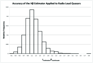
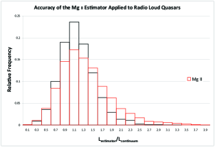
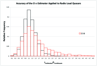
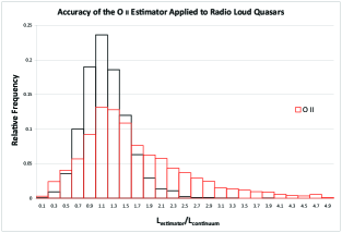
Figure 3: The histograms represent the distributions of the ratio of the estimated continuum flux to the actual continuum flux, $L_{\mathrm{estimated}}/L_{\mathrm{cont}}$ for each of the emission lines in the context of the SDSS DR7 radio loud subsample. The smallest dispersion about 1 (the most accurate estimator) is produced by the H$\beta$ based estimate in the upper left hand frame. The superior H$\beta$ fit is shown in black in the other three frames for the sake of comparison.

3 Application to Radio Loud Quasars

There are 2461 quasars in the SDSS DR7 sample, $0.4<z<0.8$, with a FIRST detection and radio loudness, $R>10$. We use this sample as a test-bed for the application of the estimators that were derived in the last section. We can check our calibrations of the bolometric correction by applying Equations (2) to (5) to each line individually and comparing the resultant $L_{\mathrm{estimated}}$ to $L_{\mathrm{cont}}$. The results are presented in Figure 3 as the probability distribution (histogram) of the ratio of estimated luminosity to measured continuum luminosity, $L_{\mathrm{estimated}}/L_{\mathrm{cont}}$. Our ”factor of two” figure of merit (i.e. $0.5<L_{\mathrm{estimated}}/L_{\mathrm{cont}}<2$) indicates that the H$\beta$ based estimate is still excellent with 94.9% of the estimates accurate to within a factor of two. The other estimators are accurate to within a factor of two in the following order, Mg II, [O III], [O II]; 86.2%, 75.1% and 67.5% of the time, respectively. Figure 3 shows that estimators based on the [OII] and [OIII] emission line strengths have a propensity to over estimate the continuum luminosity in radio loud quasars. This is in contrast to the radio quiet quasars in Figure 2, where the more errant estimates are equally likely to occur above or below ”1”. In other words, [O III] and [O II] are often much stronger than expected from the continuum luminosity alone. The implication is that the excess narrow line strength is produced by the aforementioned excited gas that is often observed aligned with the radio jets and is therefore likely to be energized by the jet (Inksip et al, 2002; Best et al, 2000; McCarthy et al, 1995). We also performed the same exercise with a cutoff at $R>20$. The results were very similar to those above, indicating that the definition of radio loudness is a negligible factor in this analysis.

We give an example of how the line strengths can be used to analyze radio loud AGN, the blazar 3C 216. We retrieve the line strengths from Lawrence et al. (1996). For H$\beta$, Mg II, [O III] and [O II], from equations (2) - (5), these line strengths yield the following estimates for $L_{\mathrm{bol}}$, $8.12\times 10^{44}$ ergs/sec, $1.23\times 10^{45}$ ergs/sec, $7.24\times 10^{45}$ ergs/sec, $1.32\times 10^{46}$ ergs/sec, respectively. 3C 216 is argued to be the one of the most kinetically dominated known quasars, with a jet power (kinetic luminosity) to $L_{bol}$ ratio $>10$ (Punsly, 2007). The broad line estimates are in good agreement, but the narrow line estimates are much larger. The results of this paper indicate that the broad lines are therefore excellent estimators of the continuum luminosity and the narrow lines are dominated by a jet contribution.

4 Conclusion

We have derived line strength based estimators for $L_{bol}$ for radio quiet quasars from the broad components of H$\beta$, Mg II, and the narrow lines, [O III] and [O II] in Equations (2) -(5). The strength of the broad component of H$\beta$ is a superior estimator of $L_{\mathrm{cont}}$ for either radio quiet or radio loud quasars since it is accurate to within a factor of two, 97.4% and 94.9% of time, respectively. The next best line strength based estimators are in order of accuracy, Mg II, [O III] and [O II]. We applied our results to radio loud quasars and found strong evidence that the narrow line based estimates are often skewed by what is likely a strong jet induced contribution. It was also demonstrated that using all four line strengths in tandem can be a useful diagnostic tool for studying the jet power, environment and accretion power in AGN.

The results of this Letter are applicable to blazars, but perhaps not to NLRGs and Seyfert 2 galaxies. There is compelling evidence that sometimes the same gas that can attenuate the nucleus in these sources can also attenuate the narrow line emission (Mulchaey et al, 1994; Kraemer et al, 2010). In general, without additional information, one does not know if the narrow line region in a particular Seyfert 2 galaxy or NLRG is attenuated or not, thus the [O III] and [O II] based estimators are not reliable in isolation. We showed in section 4 that the narrow line estimators are actually useful in the blazar context, where attenuation is not an issue. In general, narrow line based estimators are most useful if complemented by other information such as broad line luminosity or the actual continuum luminosity. For NLRGs and Seyfert 2 galaxies, the IR continuum luminosity is a valuable complement to the narrow line strengths since it is not believed to be attenuated (Fernandes et al, 2010; Ogle et al, 2006).

References

- Antonucci (1993) Antonucci, R.J. 1993, Annu. Rev. Astron. Astrophys. 31 473
- Best et al (2000) Best, P., Rottgering, H., Longair, M. 2000, MNRAS 311 1
- Boroson and Green (1992) Boroson, T. and Green, R. 1992, ApJS 80 109
- Cao and Jiang (2001) Cao, X. and Jiang, D. 2001, MNRAS 320 347
- Celotti and Fabian (1993) Celotti, A. and Fabian, A. 1993, MNRAS 264 228
- Celotti et al (1997) Celotti, A., Padovani and Ghisellini, G. 1997, MNRAS 286 415
- Dietrich et al (2002) Dietrich, M., Appenzeller, I., Vestergaard, M., & Wagner, S. J. 2002, ApJ, 564, 581
- Dong et al (2008) Dong, X., Wang, T., Wang, J., Yuan, W., Zhou, H., Dai, H., & Zhang, K. 2008, MNRAS, 383, 581
- Fernandes et al (2010) Fernandes, C. 2010, MNRAS in press arXiv:1010.0691v1
- Ghisellini et al (2011) Ghisellini, G., Tavecchio, F., Foschini, L., Ghirlanda, G. 2011, submitted to MNRAS http://xxx.lanl.gov/abs/1012.0308
- Gu et al (2009) Gu, M., Cao, X. and Jiang, D. 2009, MNRAS 396 984
- Inksip et al (2002) Inskip, K. et al 2002, MNRAS 337 1318
- Kaspi et al (2000) Kaspi, S. et al 2000, ApJ 533 631
- Kellermann & Pauliny-Toth (1969) Kellermann, K. I., & Pauliny-Toth, I. I. K. 1969 ApJ, 155, L71
- Kraemer et al (2010) Kraemer, S. et al 2010, to appear in ApJ http://arxiv.org/abs/1011.5993v1
- Lawrence et al. (1996) Lawrence, C. et al 1996, ApJS 107 541
- Maraschi and Tavecchio (2003) Maraschi, L. and Tavecchio F., 2003, ApJ 593 667
- McCarthy et al (1995) McCarthy, P., Spinrad, H., van Bruegel, W. 1995, ApJS 99 27
- Miller et al (1992) Miller, P., Rawlings, S., Saunders, R. and Eales, S. 1992, MNRAS 254 93
- Mulchaey et al (1994) Mulchaey, J. et al 1994, ApJ 436 586
- Ogle et al (2006) Ogle, P., Whysong, D. and Antonucci, R.2006 ApJ 647 161
- Punsly (2007) Punsly, B. 2007, MNRAS 374 10
- Punsly and Tingay (2006) Punsly, B., Tingay, S. 2006, ApJL 651 L17
- Rawlings and Saunders (1991) Rawlings, S., Saunders, R. 1991, Nature 349, 138
- Simpson (1998) Simpson, C. 1998, MNRASL 297 39
- Sun and Malkan (1989) Sun, W.H., Malkan, M. 1989, ApJ 346 68
- Tsuzuki et al (2006) Tsuzuki, Y., Kawara, K., Yoshii, Y., Oyabu, S., Tanabé, T., & Matsuoka, Y. 2006, ApJ, 650, 57
- Véron-Cetty et al. (2004) Véron-Cetty, M.-P., Joly, M., & Véron, P. 2004, AAP, 417, 515
- Wang et al (2004) Wang, J.-M., Luo, B, Ho, L. 2004, ApJL 615 9
- Wang et al (2009) Wang, J.-G., et al. 2009, ApJ, 707, 1334
- Willott et al (1999) Willott, C., Rawlings, S., Blundell, K., Lacy, M. 1999, MNRAS 309 1017
- Zhang et al (2010) Zhang, S. et al 2010 ApJ714 367