Spectral Sidebands and Multi-Pulse Formation in Passively Mode Locked Lasers

Abstract

Pulse formation in passively mode locked lasers is often accompanied with dispersive waves that form of spectral sidebands due to spatial inhomogoneities in the laser cavity. Here we present an explicit calculation of the amplitude, frequency, and precise shape of the sidebands accompanying a soliton-like pulse. We then extend the study to the global steady state of mode locked laser with a variable number of pulses, and present experimental results in a mode locked fiber laser that confirm the theory. The strong correlation between the temporal width of the sidebands and the measured spacing between the pulses in multipulse operation suggests that the sidebands have an important role in the inter-pulse interaction.

Introduction

Soliton-like pulses propagating in nonlinear media with periodic spatial inhomogeneity can be a source of dispersive waves that are concentrated at resonant frequencies, forming spectral sidebands, sometimes called Kelly sidebands. kelly1 . Several papers Gordon ; kelly1 ; kelly2 ; mecozzi studied the formation and of dispersive waves by solitons and their propagation in optical fibers with periodically spaced amplifiers. The same mechanism leads to the formation of sidebands in mode locked lasers, where inhomogeneities in the cavity act periodically on the pulse.

When the power of a single pulse saturates the absorber, the steady state of a passively mode locked laser tends to bifurcate into configurations where two or more pulses run in the laser cavity simultaneously. Since the early experiments that demonstrated multipulse mode locking mp1 ; mp2 ; mp3 it has been observed that the pulses display a very rich dynamics, often forming bunches, as a consequence of complex inter-pulse interactions. The interest in the dispersive waves in mode locked lasers, beyond their prominent effect on the pulse shape, arises because they have often been suggested as a means of inter-pulse interaction in multipulse mode locked lasers Grudinin_Gray ; Soto-Crespo ; Tang ; komarov . Here we focus on the role of the sidebands in multipulse mode locking.

The absorber saturation leading to multipulse steady states is often modeled by adding a quintic term to the equations of motion. In former papers stepsPRL ; stepsPRE we applied the statistical light-mode dynamics (SLD) theory to this system, and showed that multipulse mode locking is in effect a series of first order phase transitions. SLD uses the methods of statistical physics to analyze the dynamics of the interacting many body light mode system at an effective finite temperature generated by cavity noise GFPRL ; GFOC ; GGFPRE . Here we apply the SLD gain balance method PRL-2006 to derive the multipulse steady states with dispersive waves of mode locked lasers with cavity inhomogeneities.

Our theoretical analysis is based on the master equation of mode-locked soliton lasers HausReview ; KutzReview , with an additive noise term haus-mecozzi , where the inhomogeneities in the cyclic light propagation in the cavity are modeled by a periodic modulation of the gain and the saturable absorption. We first study the sidebands in a single-pulse steady state and show that, unlike free fiber sidebands, the mode locked laser sidebands reach a steady state with a well-defined bandwidth and a Lorentzian shape; in real time the dispersive waves form a wide pedestal with exponentially decaying tails. In particular we demonstrate how the overall phase of each sideband depends on the relative phase of the gain and loss modulations. The theory is firmly supported by experimental observations in mode locked fiber lasers.

Next we derive a nonlinear equation for the global steady state of the laser, that includes a number of pulses and their accompanying pedestals, by applying the gain balance principle to the pulses, sidebands, and cw components of the waveform. We find that the sideband intensity and the pedestal width increase by a large factor when the pumping is increased with a constant number of pulses, and then decrease abruptly when another pulse is formed, so that the properties of single-pulse sidebands display an oscillatory, approximately periodic, dependence on the pump power. These theoretical results are again favorably compared with experiments in a mode locked fiber laser. We conclude by considering the implication of our results on the nature of sidebands-mediated interactions.

Theoretical model

Our theoretical analysis is based on the mode-locking master equation model for soliton lasers HausReview ; KutzReview ; haus75 , where the dominant dynamical processes are chromatic dispersion and Kerr nonlinearity, whose coefficients can be nondimensionalized by an appropriate choice of units of time and power. The master equation then takes the form

$$i\partial_{z}\psi =-\partial_{t}^{2}\psi-2|\psi|^{2}\psi$$

$$+ip_{g}(z)g[\psi]\left(\psi+\gamma\partial_{t}^{2}\psi\right)$$

$$+ip_{s}(z)(s(|\psi|^{2})-l)\psi+\Gamma(z,t)$$ (1)

The first two terms on the right-hand-side are the aforementioned dispersion and Kerr nonlinearity in soliton units. The next term models the saturable gain of the laser amplifier. $g[\psi]$ is the overall gain coefficient, and the square brackets signify that $g$ depends on the entire waveform $\psi(t)$ rather than the instantaneous value of $\psi$ only, and $\gamma$ is the coefficient of parabolic spectral filtering. We will assume that the the gain saturation is slow compared to the cavity round trip time $t_{R}$, so that $g$ is determined by the overall power $P=\int\limits_{-t_{R}/2}^{t_{R}/2}|\psi|^{2}dt$ in the usual manner

$$g[\psi]=\frac{g_{0}}{1+P/P_{s}}$$ (2)

where $g_{0}$ and $P_{s}$ are the small signal gain and the saturation power, respectively.

The next term on the right-hand-side of the master equation models the fast saturable absorber with transmissivity $s(|\psi|)-l$, where $l$ is the small signal loss, and $s(0)=0$ by definition. We do not assume a particular form for the transmissivity function other than that $s(0)<l$ and that it increases linearly at zero, $s^{\prime}(0)>0$. We assume for simplicity that the saturable absorber accounts for all the losses in the cavity. The final term is a Gaussian white noise source with covariance

$$\langle\Gamma^{*}(z,t)\Gamma(z^{\prime},t^{\prime})\rangle=2T\delta(z-z^{\prime})\delta(t-t^{\prime}),$$ (3)

where the constant $T$ is the rate of internal and injected noise power. As mentioned above, the noise is a significant factor in the determination of the steady state; we conjecture that it is also an essential ingredient in the inter-pulse interaction. The sidebands are formed by the spatial inhomogeneity of the gain and loss processes in the laser, described the by $p_{g}(z)$ and $p_{s}(z)$ (respectively) that are periodic functions of the cavity roundtrip length $L$, normalized to $\frac{1}{L}\int_{0}^{L}dzp_{g,s}dz=1$.

The dominance of the dispersive effects means that the gain and loss terms in Eq. (Theoretical model) are proportional to a small parameter, and that the noise term is proportional to an independent small parameter. In spite of their smallness, the gain, loss and noise are the crucial terms for the mode locking phenomena discussed here. At the same time, they also perturb the pulse properties that are dominated by the dispersive terms; these small perturbation will be neglected.

Single-pulse side bands

We begin our analysis assuming conditions under which there is a single pulse in the cavity with fixed parameters in the steady state. Since the dominant terms in the master equations are the dispersion and Kerr effect, the pulse waveform is approximately that of a nonlinear Schrödinger (NLS) soliton. Solitons are defined by four parameters, amplitude $a$, frequency, timing and phase. The gain and loss terms in the master equation fix the frequency to zero, and we can set the timing and phase to zero by an appropriate choice of origin, so that the soliton waveform is

$$\psi_{p}(t,z)=a\textrm{sech}(at)e^{ia^{2}z}$$ (4)

The soliton waveform $\psi_{s}$ is not an exact solution of the master equation because of the gain, loss and noise terms. We therefore look for a solution of the form

$$\psi(t,z)=\psi_{p}(t,z)+\psi_{b}(t,z)+\psi_{c}(t,z)$$ (5)

that in addition to the pulse waveform, consists of the sidebands waveform $\psi_{b}$ geneated by the cavity inhomogeneities, and the continuum wave $\psi_{c}$ generated by the cavity noise. The three waveform components have different characteristic time scales: the sidebands are narrow resonances whose temporal width is, as shown below, inversely proportional to the gain-loss small parameter. This width is large compared with the pulse width, but small compared with the cavity roundtrip time—the scale of the continuum.

Both $\psi_{b}$ and $\psi_{c}$ have low peak power, and can therefore be analyzed by the linearized master equation, although their total power $\int dt|\psi_{b}|^{2}$, $\int dt|\psi_{b}|^{2}$ can be of the order $P$. The effect of noise is negligible on $\psi_{b}$, that therefore satisfies the equation

$$\partial_{z}\psi_{b} =i(\partial_{t}^{2}\psi_{b}+4|\psi_{p}|^{2}\psi_{b}+2\psi_{p}^{2}\psi_{b}^{*})$$ (6)

$$+p_{g}(z)g[\psi]\left(1+\gamma\partial_{t}^{2}\right)(\psi_{p}+\psi_{b})$$

$$+p_{p}(z)(s(|\psi_{p}|^{2})-l)(\psi_{p}+\psi_{b})$$

The right-hand-side of Eq. (6) retains terms that are of higher order of smallness than $\psi_{b}$; these terms are in effect not negligible for $|t|\gg a$ where $\psi_{p}$ is itself small, and play a crucial role in the shaping of the side bands, as shown below.

The discrete modes of the real-linear Eq. (6) express small variations of the pulse parameters haus-mecozzi ; kfg10 , while $\psi_{b}$, that consists of radiation emitted by the pulse, is a linear combination

$$\psi_{b}(t,z)=e^{ia^{2}z}\int\frac{d\omega}{2\pi}(\alpha_{\omega}(z)u_{\omega}(t)+\alpha_{\omega}(z)^{*}v_{\omega}(t)^{*})$$ (7)

of the first component of scattering states of the linear operator $L$,

$$L\begin{pmatrix}u_{\omega}\\ v_{\omega}\end{pmatrix} =(-(i+g\gamma)\omega^{2}-ia^{2}))\begin{pmatrix}u_{\omega}\\ v_{\omega}\end{pmatrix}$$ (8)

$$L\begin{pmatrix}v_{\omega}^{*}\\ u_{\omega}^{*}\end{pmatrix} =((i-g\gamma)\omega^{2}+ia^{2})\begin{pmatrix}v_{\omega}^{*}\\ u_{\omega}^{*}\end{pmatrix}$$ (9)

that acts on two-component wave functions as

$$L=\begin{pmatrix}A&B\\ B^{*}&A^{*}\end{pmatrix}$$ (10)

with

$$A=(i+g\gamma)\partial_{t}^{2}-ia^{2}+4ia^{2}{\rm sech}^{2}(at)+s(a^{2}{\rm sech}^{2}(at))$$

and $B=2ia{\rm sech}^{2}(at)$. It will be argued below that we can use approximate the space-dependent linear operator acting on $\psi_{b}$ in Eq. (6) by its space average $L$. Within this approximation the coefficients defined in Eq. (7) evolve according to

$$\partial_{z}\alpha_{\omega}= (-(i+g\gamma)\omega^{2}-ia^{2})\alpha_{\omega}+(g\alpha_{\omega}+\beta_{g\omega})p_{g}(z)$$

$$+(-l\alpha_{\omega}+\beta_{s\omega})p_{s}(z)$$ (11)

where $\beta_{g}$ and $\beta_{s}$ are the expansion coefficients of the forcing terms $g(1+\gamma\partial_{t}^{2})(a{\rm sech}(at))$ and $\big{(}s(a^{2}{\rm sech}^{2}(at))-l\bigr{)}a{\rm sech}(at)$ (respectively). As usual, the expansion coefficients are extracted by inner product with the adjoint eigenfunctions defined by

$$L^{\dagger}\begin{pmatrix}\bar{u}_{\omega}\\ \bar{v}_{\omega}\end{pmatrix} =((i-g\gamma)\omega^{2}+ia^{2})(\omega^{2}+a^{2})\begin{pmatrix}\bar{u}_{\omega}\\ \bar{v}_{\omega}\end{pmatrix}$$ (12)

$$L^{\dagger}\begin{pmatrix}\bar{v}_{\omega}^{*}\\ \bar{u}_{\omega}^{*}\end{pmatrix} =(-(i+g\gamma)\omega^{2}-ia^{2}))\begin{pmatrix}\bar{v}_{\omega}^{*}\\ \bar{u}_{\omega}^{*}\end{pmatrix}$$ (13)

normalized so that

$$\int dt(\bar{u}_{\omega}(t)^{*}u_{\omega^{\prime}}(t)+\bar{v}_{\omega}(t)^{*}v_{\omega^{\prime}}(t))=2\pi\delta(\omega-\omega^{\prime})$$ (14)

$$\int dt(\bar{v}_{\omega}(t)u_{\omega^{\prime}}(t)+\bar{u}_{\omega}(t)v_{\omega^{\prime}}(t))=0$$ (15)

Since by assumption the dispersive terms are dynamically dominant, the eigenfunctions of $L$ are close to the eigenfunctions of the linearized NLS equation kaup

$$u_{\omega}(t) =e^{i\omega t}\left(1-\frac{2i\omega e^{-at}}{(\omega+ia)^{2}}a{\rm sech}(at)+\frac{a^{2}{\rm sech}^{2}(at)}{(\omega+ia)^{2}}\right)$$ (16)

$$v_{\omega}(t) =e^{i\omega t}\frac{a^{2}{\rm sech}^{2}(at)}{(\omega+ia)^{2}}$$ (17)

$$\bar{u}_{\omega}(t) =a\frac{(\omega+ia)^{2}}{(\omega-ia)^{2}}u_{-\omega}(-t)$$ (18)

$$\bar{v}_{\omega}(t) =-a\frac{(\omega+ia)^{2}}{(\omega-ia)^{2}}v_{-\omega}(-t)$$ (19)

so that

$$\beta_{g\omega} =\frac{a}{2\pi}\frac{(\omega+ia)^{2}}{(\omega-ia)^{2}}\int dt(1+\gamma a^{2}\partial_{\theta}^{2})a{\rm sech}\theta$$ (20)

$$\quad\times e^{-i\omega t}\Big{(}1-\frac{2i\omega e^{-at}a{\rm sech}(at)+{a^{2}{\rm sech}^{2}(at)}}{(\omega+ia)^{2}}\Big{)}$$

$$\beta_{s\omega} =\frac{a}{2\pi}\frac{(\omega+ia)^{2}}{(\omega-ia)^{2}}\int dt\big{(}s(a^{2}{\rm sech}^{2}(at))-l\big{)}a{\rm sech}(at)$$ (21)

$$\quad\times e^{-i\omega t}\Big{(}1-\frac{2i\omega e^{-at}a{\rm sech}(at)+{a^{2}{\rm sech}^{2}(at)}}{(\omega+ia)^{2}}\Big{)}$$

The solution of Eq. (11) is

$$\alpha_{\omega}(z) =\int^{z}dz^{\prime}e^{(-\omega^{2}(i+g\gamma)-ia^{2})(z-z^{\prime})}$$ (22)

$$\times e^{\int_{z^{\prime}}^{z}dz^{\prime\prime}(gp_{g}(z^{\prime\prime})-lp_{s}(z^{\prime\prime}))}(\beta_{g\omega}p_{g}(z)+\beta_{s\omega}p_{s}(z))$$

As observed by Gordon and Kelly Gordon ; kelly1 ; kelly2 , the amplitudes $\alpha_{\omega}$ are driven resonantly if the nonlinear frequency shift $a^{2}+\omega^{2}$ is an integer multiple of the cavity based wavelength $\frac{2\pi}{L}$; spectrally, therefore, the dispersive waves contain a discrete set of sidebands at frequencies $\pm\omega_{n}$,

$$\omega_{n}=\sqrt{\frac{2\pi}{L}n-a^{2}}\ ,\ \ n=1,2,\ldots$$ (23)

The $n$th sideband is forced mainly by the $n$th harmonic of the gain and loss modulation functions $p_{g,l}$, but also by the $z$ dependence of the of the gain and loss terms in the exponent in Eq. (22). The latter modulation is small, however, if we make the simplifying assumption that the total net loss per roundtrip is small, so that the $z^{\prime}$ integration in Eq. (22) is effective over many roundtrips. This is the the usual assumption underlying the Haus master equation HausReview , and is also consistent with the relative weakness gain and loss processes in the dynamics dominated by the chromatic dispersion and Kerr nonlinearity that is studied here.

In this case the mean net loss in the $z^{\prime\prime}$ integration in Eq. (22) dominates over the variable parts of the gain and loss, and the latter may be neglected. The same assumption justifies the approximation of the time-dependent linear operator in Eq. (6), the equation of motion for $\psi_{b}$, by the fixed operator $L$ that was used to derive Eq. (11).

It now follows that the dispersive wave amplitudes are

$$\alpha_{\omega}(z) =\int^{z}dz^{\prime}e^{(-i(a^{2}+\omega^{2})+g(1-\gamma\omega^{2})-l)(z-z^{\prime})}$$

$$\quad\times(\beta_{g\omega}p_{g}(z)+\beta_{s\omega}p_{s}(z))$$ (24)

and defining the $n$th Fourier components $\tilde{p}_{g,n}$ and $\tilde{p}_{s,n}$ of $p_{g}$ and $p_{s}$ (respectively), the coefficients of the $n$th sideband in the steady state are

$$\alpha_{\omega,n}(z)=\frac{(\tilde{p}_{g,n}\beta_{g\omega}+\tilde{p}_{s,n}\beta_{s\omega})e^{-\frac{2\pi}{L}inz}}{l+g(\gamma\omega^{2}-1)+i(\omega^{2}-\omega_{n}^{2})}$$ (25)

We wish to characterize the sidebands by their ordinary Fourier spectrum, obtainable from Eq. (7),

$$\tilde{\psi}_{bn}(\omega,z)=e^{ia^{2}z}\int\frac{d\omega^{\prime}}{2\pi}(\alpha_{n\omega^{\prime}}(z)\tilde{u}_{\omega^{\prime}\omega}+\alpha_{n,\omega^{\prime}}(z)^{*}\tilde{v}_{\omega^{\prime}\omega}^{*})$$ (26)

where $\tilde{u}_{\omega^{\prime}\omega}=\int dte^{-i\omega t}u_{\omega^{\prime}}(t)$, and $\tilde{v}_{\omega^{\prime}\omega}$ is defined similarly. As a transform of a rapidly varying function, $\tilde{u}$ is wideband—its $\omega$ bandwidth for fixed $\omega^{\prime}$ is comparable with the soliton bandwidth—but it is also singular for $\omega=\omega^{\prime}$. The smooth part of $\tilde{u}$ generates a small deformation of the soliton waveform in Eq. (26) that is unimportant for the present purpose of characterizing the sideband spectrum. We therefore focus on the singular part $\check{u}_{\omega^{\prime}\omega}$ of $\tilde{u}_{\omega^{\prime}\omega}$ that is determined by the $\pm\infty$ asymptotes of $u_{\omega^{\prime}}$ (see Eq. (16) ) to

$$\check{u}_{\omega^{\prime}\omega}=2\pi\frac{\omega^{2}-1}{(\omega+ia)^{2}}\delta(\omega-\omega^{\prime})+\frac{4\omega a}{(\omega+ia)^{2}}\mathsf{P}\frac{1}{\omega-\omega^{\prime}}$$ (27)

where $\mathsf{P}$ denotes principal part. $\check{v}_{\omega^{\prime}\omega}=0$ since $v_{\omega}(t)$ tends to zero exponentially for $t\to\pm\infty$.

Now we can carry out the $\omega^{\prime}$ integration in Eq. (26) and obtain the spectrum of the $n$th sideband

$$\tilde{\psi}_{b,n}(\omega)=\frac{(\tilde{p}_{g,n}\beta_{g\omega}+\tilde{p}_{s,n}\beta_{s\omega})e^{i(a^{2}-\frac{2\pi}{L}n)z}}{l+g(\gamma\omega^{2}-1)+i(\omega^{2}-\omega_{n}^{2})}$$ (28)

The spectral width (half width at half maximum) of the sideband is given by $\delta\omega=(l+g(\gamma\omega_{n}^{2}-1))/2\omega_{n}\ll 1$; temporally, therefore, the dispersive wave is a pedestal of frequency $\omega_{n}$ with an exponentially decaying envelope centered at the pulse, whose decay time scale is much wider than the soliton width.

Experimentally, the sidebands appear as a series of sharp peaks in the pulse spectrum on the background of the wide soliton spectrum, (see Fig. 1). A distinctive feature of the sideband spectrum (28) is the dependence of the overall phase of the sideband on the measurement position in the cavity; as a consequence, the sideband spectrum interferes constructively or destructively with the soliton spectrum, depending on the placement of the output coupler, exhibiting a sharp notch feature for some placements as the result of destructive interference. Figs. 1–2 show the comparison between the measurement and calculation of the soliton and the first two sidebands spectrum for two cavity positions. The main qualitative discrepancy between theory and experiment is the asymmetry between the left and right sidebands that is lacking in the theory. The most likely source of this discrepancy is the assumption of a nonchirped zero frequency pulse, that only approximately holds in the experiments.

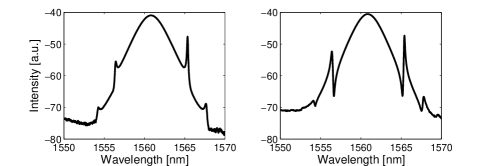
Figure 1: Measured spectra of the soliton and its sidebands, showing the notch formation. The two figures correspond to two measurement locations in the same cavity that are separated by one quarter of cavity length. These mesurements agree well with the theory.

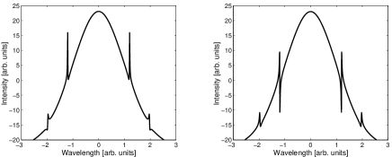
Figure 2: Theoretical calculation of the pulse and sideband spectrum with: $a=1,g=0.1,\gamma=0.01,l=0.11,s=0.1(|\psi|^{2}-|\psi^{4}|),t_{R}T=10^{-3},L=2.56,\tilde{p}_{g}=e^{i\pi/2},\tilde{p}_{s}=e^{i\pi}$. The cavity position in the left figure is $z=L/5$, and in the right is $z=0.$

The continuum component

The continuum $\psi_{c}$ is the dominant component of the waveform for most of its temporal extent, where both $\psi_{p}(t)$ and $\psi_{b}(t)$ are negligible. Therefore, the nonlinearity and interaction with the pulses are unimportant for its dynamics, and it is natural to express it in terms of the ordinary Fourier modes $\tilde{\psi}_{c}(\omega)$ that satisfy

$$\partial_{z}\tilde{\psi}_{c}=-i\omega^{2}\tilde{\psi}_{c}+p_{g}(z)g\left(1-\gamma\omega^{2}\right)\tilde{\psi}_{c}-p_{s}(z)l\tilde{\psi}_{c}+\tilde{\Gamma}(\omega,z)$$ (29)

Because the noise and continuum extend throughout the entire roundtrip time, we must use discrete frequencies to label their Fourier transform. It then follows from Eq. (3) that $\tilde{\Gamma}(\omega,z)==\int dte^{-i\omega t}\Gamma(t,z)$ has zero mean and correlation function $\langle\tilde{\Gamma}(\omega,z)\tilde{\Gamma}^{*}(\omega^{\prime},z^{\prime})\rangle=2Tt_{R}\delta(z-z^{\prime})\delta_{\omega,\omega^{\prime}}$. The solution of Eq. (29) is similar to (22), and by the same arguments that lead to Eq. (Single-pulse side bands) we again approximate the integrand in the exponent by its mean value. The resulting expression implies that $\langle\tilde{\psi}_{c}(\omega)\rangle=0$ and

$$\langle\tilde{\psi}_{c}(\omega)\tilde{\psi}_{c}^{*}(\omega^{\prime})\rangle=\frac{t_{R}T\delta_{\omega,\omega^{\prime}}}{l+g(\gamma\omega^{2}-1)}$$ (30)

Gain balance and multipulse sidebands

In the analysis presented so far, the pulse parameters and the overall saturated gain $g$ were assumed fixed and given. In the steady state these are variables, determined along with the number of pulses as a solution of the optical equation of motion Eq. (Theoretical model). Since the equations of motion are random, the result is a statistical steady state. In previous works GGFPRE ; PRL-2006 , statistical light-mode dynamics (SLD) theory was used to study this problem, and applied to multipulse mode locking in stepsPRL ; stepsPRE . The global mode locking analysis determines in particular the properties of the sidebands, and in this way allows us to reach our goal of describing the width and power of the sidebands as a function of the laser parameters.

Here we study the statistical steady state by the gain balance method, deriving equations of motion for the power in the three components of the optical waveform, that is, the power $P_{p}$ in the pulse waveform that comprises zero or more pulses, the sideband power $P_{b}$, and the continuum power $P_{c}$. The three waveform components are characterized by well-separated time scales, and the total power can therefore be calculated as a sum of the powers of the individual components. One looks for a steady state where the three components are subject to the same saturated gain, and finally the gain itself is determined self-consistently from Eq. (2).

We will assume that the multipulse waveform is of the simplest kind stepsPRL that is also the most commonly observed experimentally, consisting of $k$ pulses of equal amplitude $a$. In the equation of motion for the pulse amplitude we may neglect the noise term in the master equation, and use the results of soliton perturbation theory Gordon ; karpman to write

$$\frac{da}{dz} =\mathop{\mathrm{missing}}{Re}\int dt\psi_{p}^{*}\bigl{(}gp_{g}(z)(1+\gamma_{g}\partial_{t}^{2})\psi_{p}$$

$$\qquad+p_{s}(z)(s(|\psi_{p}|^{2})-l)\psi_{p}\bigr{)}$$

$$=2gp_{g}(z)a(1-\frac{\gamma}{3}a^{2})+p_{s}(z)(2s_{a}(a)-2l)a$$ (31)

where

$${s}_{a}(a)=\frac{1}{2a}\int s(a^{2}{\rm sech}^{2}(at))a^{2}{\rm sech}^{2}(at)dt$$ (32)

The pulse amplitude changes periodically during its propagation in the cavity; for our purposes we need the mean pulse amplitude $\bar{a}(z)=\frac{1}{L}\int a(z+z^{\prime})dz^{\prime}$. Under the assumption of weak gain and loss processes the dynamics of $\bar{a}$ is obtained by the space average of Eq. (31), that gives in the steady state

$$g(1-\frac{\gamma}{3}\bar{a}^{2})-l+s_{a}(\bar{a})=0$$ (33)

This equation, together with $P_{p}=2k\bar{a}$, determines the pulse part of the gain balance.

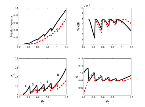
Figure 3: The theoretical calculated values of the sidebands peak intensity, width, and total power $P_{b}$ along with the saturated gain coefficient $g$ as a function of the small signal gain $g_{0}$. The same parameters as in Fig. 2 were used in the calculation, except that $\gamma=10^{-3}$ and $P_{S}=1$. Two noise injection rate values are shown: $T=10^{-3}$ in continuous black line, and $T=3\times 10^{-3}$ in dashed red line. The number of pulses is indicated. All values are given in natural soliton units.

Next, we calculate the power carried by the pedestals of the pulses. Each pulse generates a series of sidebands of the form given by Eq. (28). The sidebands power is dominated by the leading, $n=\pm 1$ sidebands; since the different pulses that act as sources for the sidebands are not phase locked, we treat them as incoherent sources, and accordingly calculate the total sidebands power, as the sum of the individual sideband powers. The resulting expression is

$$P_{b}=k\frac{|\tilde{p}_{g,1}\beta_{g\omega_{1}}+\tilde{p}_{s,1}\beta_{s\omega_{1}}|^{2}}{2\omega_{1}(l+g(\gamma\omega_{1}^{2}-1))}$$ (34)

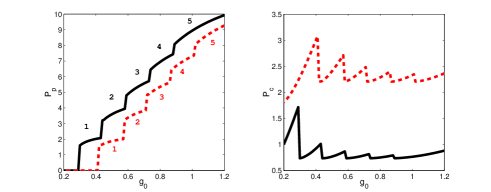
Figure 4: The theoretical calculated values of the total pulse power $P_{p}$ and noise power $P_{n}$ as a function of the small signal gain $g_{0}$. The same parameters as in Fig. 3. The number of pulses is indicated. All values are given in natural soliton units.

Finally the mean power of the the continuum is not changed by the presence of the sidebands, and is therefore given by the expression derived in njp

$$P_{c}=\frac{Tt_{R}}{2\sqrt{g\gamma(l-g)}}$$ (35)

smaller than the pulse power $2a$, so that $P_{c}$ is of the same order of magnitude as $P_{s}$.

We now substitute $P=P_{s}+P_{b}+P_{c}$ into Eq. (2) and obtain a nonlinear equation for the saturated gain $g$ that is easy to solve numerically. Once we know the value of $g$ we obtain the steady state solution of the entire waveform. The steady state equation can have several solutions with different numbers of pulses $k$. In such cases the laser waveform can exist in several states stepsPRL ; stepsPRE , in a similar manner to the existence of metastable phases in thermodynamic systems undergoing first order phase transitions. The laser then exhibits hysteresis—its actual state depends on the history.

Figs. 3–4 show the results of the calculation as the small signal gain $g_{0}$ is varied. For very low gain the waveform is pure continuum, and its energy increases with the gain. When $g_{0}$ is increased beyond a certain threshold, a pulse forms and along with it also a dispersive wave. Because of gain saturation, the net gain must abruptly decrease, and along with it also the continuum component. Further increase of $g_{0}$ will mainly increase the sidebands and the continuum components, and slightly change the pulse amplitude, until the second threshold is met, and then the continuum as well as the sidebands power abruptly decrease again. This process then continues periodically when further pulse creation thresholds are reached. In addition, as the pumping is increased between pulse creation thresholds, the saturated gain increases, so that the net loss decreases and the sidebands become spectrally narrower, and accordingly temporally wider.

The theoretical predictions of the global sidebands characteristics agree well with experimental observation summarized in Fig. 5, made on a fiber ring laser mode locked by polarization rotation as described in stepsPRE . In both graphs the sideband width displays roughly periodic sawtooth behavior and the total sidebands energy a sawtooth behavior with an increasing linear bias. There is somewhat worse agreement in the peak intensity, but this quantity is sensitive to interferometric enhancement and reduction as explained above.

In both theory and experiments the spectral width of the sidebands narrows with increasing pumping between pulse creation thresholds, implying a temporal widening of the pedestals. This widening shows a striking correlation with the increase of the inter-pulse distance, suggesting that the sidebands play a role in the inter-pulse interactions Grudinin_Gray ; Soto-Crespo .

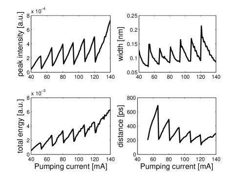
Figure 5: The measured sideband spectrum characteristics: peak power, spectral width, and total energy, and the distance between adjacent pulses in states with two or more pulses.

Conclusions and outlook

We presented a fundamental theory of the formation of sidebands and their effect on the statistical steady state in multipulse mode-locked soliton lasers, that explains the main experimental observations, including the dependence of the sideband spectrum on the measurement position in the cavity, the growth of the sideband energy and temporal width when pumping is increased, and the abrupt attenuation of the sidebands when a new pulse is created in the cavity. We also found strong correlations between the temporal width of the sidebands and the spacing between adjacent pulses in pulse bunches, giving further evidence for the role of the sidebands in inter-pulse interaction. However, the most natural conclusion from our observation is that the sidebands generate repulsive interactions, and that additional attractive interactions are needed to explain the ubiquitous formation of pulse bunches. Moreover, the phase and timing jitter of the pulses leads us to conjecture that the mechanism of interaction is incoherent. We postpone the in-depth study of these question to a future publication.

Acknowledgments: This research was supported by the Israel Science Foundation.

References

- (1) S. M. J. Kelly, Elec. Lett. 28, 806 (1992).
- (2) J. N. Elgin and S. M. J. Kelly, Opt. Lett. 18, 787 (1993).
- (3) J. P. Gordon, J. Opt. Soc. Am. B 9, 91 (1992).
- (4) F. Matera, A. Mecozzi, M. Romagnoli, and M. Settembre, Optics Letters, Vol. 18, Issue 18, pp. 1499-1501 (1993)
- (5) M. Nakazawa, E. Yoshida, Y. Kimura Appl. Phys. Lett. 59, 2073 (1991)
- (6) D. J. Richardson, R. I. Laming, D. N. Payne, M. W. Phillips, and V. J. Matsas, Electron. Lett. 27, 730 (1991)
- (7) A. B. Grudinin, D. J. Richardson, and D. N. Payne, Electron. Lett. 28, 67 (1992)
- (8) D. Y. Tang et al., Phys. Rev. E 72, 016616 (2005).
- (9) J.-M. Soto-Crespo, N. Akhmediev, Ph. Grelu and B. Belhache, Opt. Lett. 28, 1757, (2003).
- (10) A. B. Grudinin and S. Gray, J. Opt. Soc. Am. B 14, 144 (1997).
- (11) A. Komarov, K. Komarov, and F. Sanchez, Phys. Rev. A 79, 033807 (2009)
- (12) B. Vodonos, R. Weill, A. Gordon, A. Bekker, V. Smulakovsky, O. Gat and B. Fischer, Phys. Rev. Lett. 93, 153901, (2004).
- (13) R. Weill, B. Vodonos, A. Gordon, O. Gat and B. Fischer, Phys. Rev. E 76, 031112, (2007).
- (14) A. Gordon and B. Fischer, Phys. Rev. Lett. 89, 103901, (2002).
- (15) A. Gordon and B Fischer, Opt. Commun 223, 151 (2003).
- (16) O. Gat, A. Gordon, and B. Fischer, Phys. Rev. E 70, 046108, (2004).
- (17) M. Katz, A. Gordon, O. Gat and B. Fischer, Phys. Rev. Lett. 97, 113902, (2006).
- (18) H. A. Haus, IEEE J. Sel. Top. Quant. 6 1173 (2000)
- (19) J. N. Kutz, SIAM Review, 49, 629 (2006).
- (20) H. A. Haus and A. Mecozzi, IEEE J. Quantum Electron. 29, 983 (1993).
- (21) H. A. Haus, J. Appl. Phys. 46, 3049 (1975)
- (22) M. Katz, O. Gat, and B. FischerOpt. Lett. 35, 297 (2010).
- (23) D. J. Kaup, Phys. Rev. A 42, 5689 (1990)
- (24) V. I. Karpman, Phys. Scr. 20, 462 (1979)
- (25) O. Gat, A. Gordon and B. Fischer, New J. Phys. 7, 151 (2005).