The power of Bayesian evidence in astronomy

Abstract

We discuss the use of the Bayesian evidence ratio, or Bayes factor, for model selection in astronomy. We treat the evidence ratio as a statistic and investigate its distribution over an ensemble of experiments, considering both simple analytical examples and some more realistic cases, which require numerical simulation. We find that the evidence ratio is a noisy statistic, and thus it may not be sensible to decide to accept or reject a model based solely on whether the evidence ratio reaches some threshold value. The odds suggested by the evidence ratio bear no obvious relationship to the power or Type I error rate of a test based on the evidence ratio. The general performance of such tests is strongly affected by the signal to noise ratio in the data, the assumed priors, and the threshold in the evidence ratio that is taken as ‘decisive’. The comprehensiveness of the model suite under consideration is also very important. The usefulness of the evidence ratio approach in a given problem can be assessed in advance of the experiment, using simple models and numerical approximations. In many cases, this approach can be as informative as a much more costly full-scale Bayesian analysis of a complex problem.

1 INTRODUCTION

The apparatus of Bayesian evidence has been proposed as the preferred means of answering questions concerning model complexity in astronomy (e.g. Trotta 2008). Astronomers commonly wish to decide whether a given model fits a dataset adequately, or whether there is a need for additional degrees of freedom. Bayesian methods are attractive in this context because they expose any assumptions or prior information being used, and permit a clear statement of the questions that scientists actually ask of their data (e.g. Jaynes 2003). They have been used extensively in the difficult problems of inference that arise in cosmology (e.g. Hobson et al. 2010), and also in the complex, multi-parameter modelling needed for the discovery of exoplanets (e.g. Gregory 2005). Astronomy is by no means the only area of science where these methodological questions are posed or where Bayesian methods are proposed as the solution; but the astronomical literature on the topic raises some issues worth treating in context.

Bayesian methods give a transparent framework for model choice, in which it is necessary to define the set of competing models explicitly and exhaustively; Bayes’ theorem then gives the probability of any particular model being correct. Integrating this Bayesian probability over the parameter space associated with the models (as detailed below in Section 2) then yields an overall ratio of odds for particular classes of models: the ‘evidence ratio’. The requisite multi-dimensional integrations over the parameter spaces of the models present a computational challenge, and astronomers have made contributions to the development of these techniques. The refinement of Markov Chain Monte Carlo methods for the evaluation of multi-dimensional integrals is an example (Skilling 2004; Mukherjee, Parkinson & Liddle 2006; Feroz, Hobson & Bridges 2009). Numerical Bayesian are establishing themselves as a default approach, via public-domain packages such as CosmoMC (http://cosmologist.info/cosmomc/) and MultiNest (http://ccpforge.cse.rl.ac.uk/gf/project/multinest/).

Accepting the evidence ratio methodology, some authors have gone further and attempted to place a quality measure on future experiments according to the expected evidence ratio values that they are predicted to yield for given decision problems (Trotta 2007b; Heavens, Kitching & Verde 2007). What has been missing from this discussion, however, is an assessment of the statistical power of the evidence ratio: different realizations of data for a given experimental configuration will yield different values of the evidence ratio, and we need to know how often the method will discriminate correctly between models, and how often it will fail. This is a frequentist view of a Bayesian tool, but there is no conflict: the evidence ratio is a statistic generated from a dataset, so it is legitimate to ask how it will behave under repeated trials.

We will discuss several examples where the evidence ratio can be used for model choice, and we will examine the statistical variation that results from different realizations of the data. The variation is considerable, and we argue that this is likely to be generally true. This suggest caution in the use of evidence ratios, but it suggests that simplified methods can be used to compute evidence ratios and check their robustness.

Notwithstanding these caveats, we do advocate a more widespread use of the evidence ratio technique in astronomy. Bayesian methods are currently usually employed on complex, high-value problems; but astronomers are also interested in simpler model choice problems where the Bayesian techniques have much to offer and are much easier to use (at least in an approximate way). It is feasible to experiment with these simpler cases and get a good sense of the robustness of the method. Approximate Bayesian methods may often be as good as is justified by the data.

2 THE BAYESIAN EVIDENCE RATIO METHOD

Suppose we have just two models $H_{0}$ and $H_{1}$, associated with sets of parameters $\vec{\alpha}$ and $\vec{\beta}$. For data $D$, Bayes’ theorem gives the posterior probabilities of the models and their parameters:

$$P(H_{0},\vec{\alpha}\mid D)\propto P(D\mid H_{0},\vec{\alpha})\times P(\vec{\alpha}\mid H_{0})\times P(H_{0})$$ (1)

and

$$P(H_{1},\vec{\beta}\mid D)\propto P(D\mid H_{1},\vec{\beta})\times P(\vec{\beta}\mid H_{1})\times P(H_{1}).$$ (2)

Here the priors are, for instance, $P(\vec{\alpha}\mid H_{0})$, the probability distribution of the parameters given model $H_{0}$, multiplied by the prior probability of the model class $H_{0}$ itself. We can often avoid the (common) normalizing factor required in these equations. It divides out whenever we take the ratio to form relative probabilities or ‘odds’.

The restriction to two models is not fundamental. Often $H_{0}$ is the ‘null’ or default hypothesis and is relatively simple and well understood. It is vital that $H_{1}$ be reasonably comprehensive, covering a range of possibilities, as otherwise the evidence ratio formalism may result in high odds in favour of one of the models when both are a poor fit.

The term ‘model’ can commonly be applied to each distinct point in parameter space, but a distinct question is how reasonable a given class of model is in the face of some data. When we discuss ‘model selection’, we are thus interested in the general viability of $H_{0}$ or $H_{1}$, irrespective of the exact value of their parameters. Integrating out the parameters gives the posterior probabilities of $H_{0}$ and $H_{1}$, conditional on the data. The ratio of these probabilities is the posterior odds, ${\cal O}$:

$${\cal O}\equiv\frac{P(H_{1}\mid D)}{P(H_{0}\mid D)}=\frac{\int P(D\mid H_{1},\vec{\beta})P(\vec{\beta}\mid H_{1})\,d\vec{\beta}}{\int P(D\mid H_{0},\vec{\alpha})P(\vec{\alpha}\mid H_{0})\,d\vec{\alpha}}\times\frac{P(H_{1})}{P(H_{0})}.$$ (3)

We assume that our set of possible models is exhaustive, so that $P(H_{1}\mid D)+P(H_{0}\mid D)=1$, the probability of $H_{0}$ is

$$P(H_{0}\mid D)=\frac{1}{1+{\cal O}}.$$ (4)

For more than two models, this does not hold, but ${\cal O}$ always gives the relative probabilities of any two models.

The odds ratio ${\cal O}$ updates the prior odds on the models, $P(H_{1})/P(H_{0})$, by a factor that depends on the data:

$$({\rm Posterior\ odds})=({\rm evidence\ ratio})\times({\rm prior\ odds}),$$ (5)

or

$${\cal O}={\cal E}\times{\cal PO},$$ (6)

where the definition of the evidence ratio ${\cal E}$ involves integrals over the likelihood function times the priors on the parameters:

$${\cal E}=\frac{\int{\cal L}(\vec{\beta}\mid H_{1})\,P(\vec{\beta}\mid H_{1})\,d\vec{\beta}}{\int{\cal L}(\vec{\alpha}\mid H_{0})\,P(\vec{\alpha}\mid H_{0})\,d\vec{\alpha}}.$$ (7)

The priors have to be properly normalized and may be quite different for $H_{0}$ and $H_{1}$. If the models in question are also hard to calculate, the computational problem is large.

A decision about which model to prefer thus requires both the evidence ratio and the prior ratio. The prior ratio is often taken as unity, but this is not always justified. For example, one might be reluctant to accept (say) $H_{1}$ with 100 free parameters if $H_{0}$ had no free parameters. The evidence ratio contains a different penalty for unnecessary complexity in the models: models are penalized if a small part of their prior parameter range matches the data. This is often called the Ockham ‘factor’ (e.g. p348 of Mackay 2003), although it is not usually an explicit multiplicative penalty based on the number of parameters.

In this paper, we will always take the prior ratio to be unity, in the interests of brevity. This allows us in our examples to use ‘evidence ratio’ and ‘odds’ interchangeably, the latter being often more illuminating.

The roles of the priors on the parameters, and the Ockham penalty, have been extensively discussed. Recent examples include Trotta (2008) and Niarchou, Jaffe & Pogosian (2004). In hard problems, the prior and the likelihood can be of similar importance in determining the value of the integral, and their product may be multi-peaked or otherwise pathological.

Many interesting cases are however much easier. The first examples we will discuss can be solved analytically. More generally, if our data are informative, the likelihood function may be considerably narrower than the prior. The priors can then be approximated by constants over the relevant range of the parameters in the evidence integrals. Furthermore, in simple cases the integrand may be close to Gaussian around its peak, in which case the consequent integration of a multivariate Gaussian can be done analytically:

$$\int L(\vec{\alpha})\,P(\vec{\alpha})\,d\vec{\alpha}\simeq\frac{(2\pi)^{m/2}}{\sqrt{\mid\mbox{det}({\cal H})\mid}}\,L(\vec{\alpha}^{*})\,P(\vec{\alpha}^{*}),$$ (8)

where $\vec{\alpha}^{*}$ is the value at the peak of the likelihood, $\cal{H}$ is the Hessian matrix of second derivatives of the log of the likelihood at the peak, and $m$ is the number of parameters. This equation is known as the Laplace approximation, or the method of steepest descent (see e.g. p341 of Mackay 2003).

The integration then reduces to the less laborious task of finding the maximum posterior probability, and evaluating the matrix $\cal{H}$. Averaging $\cal{H}$ over many realizations of the data yields the Fisher matrix, which may be inverted to yield an approximate prediction for the covariance matrix of the parameters (e.g. Tegmark, Taylor & Heavens 1997).

The Laplace approximation may not be valid, since the posterior may not be Gaussian near its peak, or there may be multiple peaks of similar height. The applicability of the approximation thus needs to be checked, at least via inspection of the posterior, or via comparison with an alternative robust means of integration, such as Monte Carlo. Monte Carlo methods can be also used to quantify the robustness of the evidence ratio for different realizations of the data. In addition to providing possible indications of multimodality in the posterior, such an approach can also probe the stability of the evidence ratio against systematic error at plausible levels.

3 THE EVIDENCE AS A STATISTIC

3.1 Repeated experiments

Posterior odds on hypotheses can be obtained from a given dataset without ever having to consider whether the experiment could be repeated. This is the well-known advantage of Bayesian reasoning over the frequentist approach. Yet many kinds of experiment can be and are repeated many times: observations in astronomical surveys are an obvious example. In these circumstances, the Bayesian evidence is a statistic that can be computed from a given dataset, and it is hard not to wonder what value might have been obtained had our dataset been a different realization of the experimental process. Clearly if we know the likelihood function, which we must do to compute the evidence, then we must be able to generate other possible realizations of the data.

To make a decision based on the posterior odds, a threshold is set at some value of posterior odds, such as the ‘decisive’ $\ln{\cal E}=5$ value advocated by Jeffreys (1961). We may ask how often such a strategy might lead us to make an incorrect decision. Conversely, it is useful to know if a given experimental setup is likely to yield data good enough to exceed the decision threshold and ‘detect’ the more complex model in cases where it is true.

Suppose further that the evidence ratio turns out to be a ‘noisy’ statistic, in the sense that its distribution is very broad: in this case, there is little point in devoting excessive effort in computing the evidence ratio very precisely. Given that practical computations can involve difficult integrations over spaces of very high dimensionality, this is worth knowing.

The notion of ‘repeated trials’ needs clarification. In the simplest case, the fluctuations in our data arise in the measurement process, while the object or process we are observing has fixed parameters. A distinct case arises when we make repeated measurements of objects or processes that are different on each repetition. This often happens when we are observing samples and wish to make statements about properties of whole populations. In this case, extra variance enters, often called cosmic variance. An elementary example is the distinction between repeated (noisy) measurements of the flux of a single galaxy, or a series of measurements where a different galaxy is observed on each occasion. In the latter case, we will have a prior distribution for the true flux of a randomly selected galaxy, and the data we obtain in a given measurement could be modelled by drawing a random number from this prior distribution, and then adding noise.

In dealing with the evidence ratio for repeated trials, we will thus use the prior twice. The standard Bayesian approach regards the data as being fixed specific numbers, and the prior enters only when we average the likelihood function over the prior to obtain the posterior probabilities. However, when we view the Bayesian outputs as statistics, we have to treat the data as random variables, whose distribution will depend on the values of the parameters for which we have a prior. The probability distribution of the evidence ratio involves the data, and so depends on the unknown parameters that are the argument of the prior. We can eliminate these parameters by a further integration over the prior, in effect, marginalizing the distribution of the evidence ratio to obtain its probability distribution independent of parameters.

3.2 Neyman-Pearson Analysis

Suppose we have the posterior probabilities or posterior odds for our competing models. These will vary with different realizations of the data. What do we do with these probabilities or odds? This is not a question that can be answered by probability theory but it can be illuminated by it.

One approach is to set a threshold in the odds, effectively taking one decision if our experiment gives posterior odds above the threshold, and another if they lie below. This general idea was introduced to classical statistics by Neyman and Pearson. A Bayesian approach is to emphasize the posterior probabilities or odds as a complete summary of our state of knowledge after the experiment, and to resist further interpretation. There are parallels here with the long history of controversy in classical statistics about the Neyman-Pearson approach versus Fisher’s significance testing. Fisher recognized the utility of the Neyman-Pearson method in industrial acceptance testing but regarded it as too “wooden” to be useful in the ill-defined and creative processes of science (Fisher 1956). His detestation of Bayesian methods aside, Fisher would perhaps have been sympathetic to the idea that posterior probabilities should be carried forward intact through the processes of science; he took much the same view of the results of his tests of significance.

We believe that binary choice between alternatives is a relevant process in astronomy. The high cost and complexity of many astronomical research projects requires a difficult decision on when to commit to construction, which is irrevocable once made. More generally, there is the whole issue of how a community develops a consensus. The Bayesian ideal of a set of individuals each interpreting the evidence ratio in the their own way is hardly realistic: rather, some pre-defined level of proof is needed – a threshold in evidence ratio, in short. We will therefore apply a Neyman-Pearson style of analysis to the evidence ratio, despite recognizing that this is not a unique assessment of is utility.

Given the distribution of the evidence ratio ${\cal E}$ under two competing hypotheses, we can ask how well the statistic performs. A Neyman-Pearson analysis proceeds by defining a critical threshold in the test statistic, say ${\cal E}_{c}$. If ${\cal E}<{\cal E}_{c}$, we do not see any reason to reject the simpler null hypothesis $H_{0}$, and it is accepted. If ${\cal E}>{\cal E}_{c}$, there is good reason to prefer the more complex hypothesis $H_{1}$ and $H_{0}$ will be rejected. A common ‘decisive’ choice for the critical threshold is $\ln{\cal E}_{c}=5$, corresponding to odds in favour of $H_{1}$ of 148:1 (Jeffreys 1961; Jaynes 2003). The common restriction to two models is not critical, since we can always add the posterior probabilities for $N$ alternative models and consider this to be a single alternative. This yields sensible answers, even in the case where all $N$ models fit the data about as well as $H_{0}$: if $N>148$, we would then decide that there was decisive evidence against $H_{0}$, even though $H_{0}$ fitted as well as any model. This simply reflects our assumption that all models are equally likely a priori.

In the Neyman-Pearson approach, there are two ways in which an incorrect conclusion might be reached:

1. Type I Error (False Positive). $H_{0}$ is true, but we are unlucky enough to get a high value of ${\cal E}$ above ${\cal E}_{c}$, so $H_{0}$ is incorrectly rejected. The Type I error rate is $\alpha\equiv P({\cal E}>{\cal E}_{c}\mid H_{0})$.

2. Type II Error (False Negative). $H_{1}$ is true, but a value of ${\cal E}$ below the threshold is found, so we fail to ‘detect’ the need for a more complex model. The power is 1-Type II error rate and so is ${\cal P}\equiv P({\cal E}<{\cal E}_{c}\mid H_{1})$.

The power of the test is defined as the probability that we will correctly pick $H_{1}$ when it is true – i.e. it is unity minus the probability of a Type II error. There is the usual trade-off: if we conservatively use a high threshold, we reduce the chance of a Type I error, but we also reduce the power of the test because we are increasing the probability of a Type II error. The power is less often discussed in astronomy, because alternative hypotheses are frequently ill-defined. However, the notion of these alternatives is inherent in the Bayesian method.

An example might be a case where we calculate a statistic, say chi-square, to evaluate the goodness of fit of a model $H_{0}$. From this we may compute what is often called the $p$-value, the probability of exceeding the value of chi-square we actually obtained, assuming $H_{0}$ to be correct. This is classical significance testing. In the Neyman-Pearson method, we would fix in advance a critical value of chi-square, corresponding (say) to $p=0.05$. If we exceed this critical level (by any amount) we reject $H_{0}$; if we only have two models, we then accept $H_{1}$.

The Neyman-Pearson binary decision rule avoids the paradoxical issue of the relation between $p$ and $P(H_{0}\mid D)$, which has been pondered by a long series of authors (Lindley 1957; Jeffreys 1961 and others cited in Berger & Sellke 1987; Sellke, Bayarri & Berger 2001). Paradoxes arise because we might think that if we obtained a small value of $p$, it would follow that $H_{0}$ was unlikely to be correct. While this is not a rigorous interpretation of the meaning of $p$, successive authors have calibrated $p$ for a range of models, and found that $p<P(H_{0}\mid D)$. This situation can be understood if we select outcomes with given $p$ from an ensemble of repeated experiments in which $H_{0}$ and $H_{1}$ are equally likely. At one extreme, the two models may be rather similar, in which case an outcome with any $p$ is equally probable on either model; if the models are extremely different, $H_{1}$ might always yield $p\ll 1$, so observing e.g. $p=0.05$ could in fact provide strong reason to prefer $H_{0}$. Thus $H_{0}$ can be more likely than the value of $p$ might seem to suggest, and a calibration of $p$ is required: without this, it is hard to know what decisions to take on the basis of $p$. This discussion has continued since Fisher introduced $p$ and the idea of significance testing.

The Neyman-Pearson approach, by contrast, is quite clear about how statistics should be used to take decisions and it is for this reason that we analyze the performance of the Bayesian evidence ratio using the concepts of Type I error rate and power. Our analytical models are the same as those discussed before (Lindley 1957; Jeffreys 1961, for example) and we reproduce the $p<P(H_{0}\mid D)$ effect. But this is not our focus; our interest is in showing how the Bayesian evidence ratio performs, as a basis for decision, under repeated trials.

An advantage of the Neyman-Pearson approach is that because there is a clear decision rule, the risks are also clear. For example, if there is a cost of some sort associated with wrongly rejecting the null hypothesis, then the threshold can be set to minimize this. As we shall see, however, this also affects the power – and may affect the likely pay-off of correctly choosing the alternative.

The Neyman-Pearson lemma tells us that a statistic based on the likelihood ratio will be the best one to use as a basis for decision. The evidence ratio is quite closely related to a likelihood ratio and so this is another reason for examining its performance from a Neyman-Pearson point of view.

We also note that the Neyman-Pearson approach can also be assessed in a Bayesian way: we might ask, what is the probability of (say) $H_{1}$, given that I have just obtained ${\cal E}>{\cal E}_{c}$? This quantity, $P(H_{1}\mid{\cal E}<{\cal E}_{c})$, is called the ‘positive predictive power’ in medical literature. It is related by Bayes’ Theorem to the Type I and Type II error rates, and the prior odds ratio on $H_{1}$ and $H_{0}$:

$${\rm PPP}=\frac{\Theta{\cal P}}{\alpha+\Theta{\cal P}},$$ (9)

in which $\alpha$ is the false positive rate, ${\cal P}$ is the power, and $\Theta$ is the prior odds on $H_{1}$. Evidently the use of the PPP requires us to set a threshold in advance on our test statistic, much as in the Neyman-Pearson approach. We might then pose similar counterfactual questions such as, if we have obtained ${\cal E}<{\cal E}_{c}$ and we then choose $H_{1}$ with probability PPP, what might our loss be if $H_{0}$ is true?

4 GAUSSIAN EXAMPLES

We will now examine two contrasting Gaussian examples. In the first, both priors are very narrow and the evidence ratio acts in the same way as a classical statistic for model choice. In the second we have one prior much wider than the other. The evidence ratio method now diverges strongly from a classical alternative and the role of the Ockham factor is apparent. In both cases we will see how finite amounts of data reduce the effectiveness of decisions based on thresholds in the evidence ratio.

We have $N$ data values, $X_{i}$, which may have arisen via one of two models:

1. Independent drawings from a Gaussian of unit standard deviation and mean zero.

2. Independent drawings from a Gaussian of unit standard deviation and mean $\mu$.

As usual, we assume that these two possibilities are a priori equally probable. This is a case where the two models are nested: model 1 is a special case of model 2 ($\mu=0$).

In astronomical terms, this situation might correspond to a (one-dimensional) Gaussian source in the zero-background limit (X-ray astronomy). The observed $N$ photon locations are $X_{i}$, and we wish to see if there is evidence that the source is offset from some pre-determined position. As noted, there are various possibilities one may wish to test. One is that the source is supposed to be at one of two definite positions, both of which we know. Another is that the source is either at one definite position, which we know, or it is located ‘somewhere else’. Here we put a Gaussian prior on the alternative position and so know the parameters of that prior (most interestingly, the spread). We now deal with these cases in turn.

4.1 Example 1

The models $H_{0}$ and $H_{1}$ hypothesize that the $N$ data $X_{i}$ are drawn from unit Gaussians of mean zero and mean $\mu$ respectively. The evidence ratio ${\cal E}$ is then very simple:

$$-2\ln{\cal E}=\sum_{i=1}^{N}(X_{i}-\mu)^{2}-\sum_{i=1}^{N}X_{i}^{2}=N(\mu^{2}-2M\mu),$$ (10)

where $M$ is the mean of the $N$ samples. Clearly $M$ will be Gaussian, of variance $1/N$, under either hypothesis, and so the logarithm of the evidence ratio is also Gaussian. This means that the evidence ratio will have considerable scatter, provided $N\mu^{2}\gg 1$.

Our decision procedure is to reject $H_{0}$ (and therefore accept $H_{1}$) when ${\cal E}$ exceeds some threshold ${\cal E}_{c}$. This occurs when $M$ exceeds

$$M_{0}=\frac{\ln{\cal E}_{c}+N\mu^{2}/2}{N\mu}.$$ (11)

We make a Type I error (incorrectly rejecting $H_{0}$) when $M$ exceeds this threshold and $H_{0}$ is true. The probability of this is the probability that $M$ exceeds $M_{c}$ when $M$ is a Gaussian of mean zero and variance $1/N$, which is

$$P({\rm type\ I})=\frac{1}{2}\left(1-\mbox{erf}\left(\frac{(2\ln{\cal E}_{c}+N\mu^{2}}{2\sqrt{2N}\mu}\right)\right)$$ (12)

We make a Type II error (incorrectly failing to reject $H_{0}$) when $M$ is less than $M_{c}$ and $H_{1}$ is true. The probability of this is

$$P({\rm type\ II})=\frac{1}{2}\left(1-\mbox{erf}\left(\frac{(-2\ln{\cal E}_{c}+N\mu^{2}}{2\sqrt{2N}\mu}\right)\right)$$ (13)

Fig. 1 illustrates the possibilities. From these expressions we can calculate curves of power versus Type I error level, in which $\mu$ and $N$ are parameters. These are shown in Fig. 2.

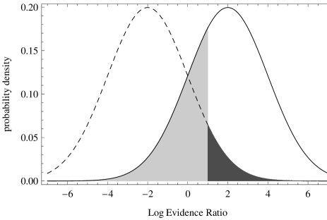
Figure 1: The probability distributions of $\ln{\cal E}$ under $H_{0}$ (left) and $H_{1}$ (right), assuming $N=4$ and $\mu=1$. For the arbitrary choice $\ln{\cal E}_{c}=1$, the dark shaded area gives the Type I error rate, and the light shaded area gives the Type II error rate.

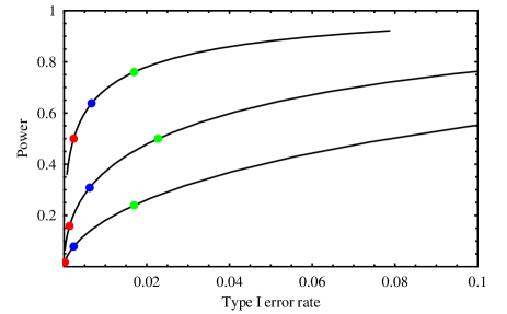
Figure 2: Parametric curves of the power of the evidence ratio test for example 1, as a function of the probability of Type I error, with the parameter being the evidence ratio. Curves are shown for $\mu=1$ and $N=2$ (lowest curve), with $N$ increasing for each curve by a factor 2. The dots show evidence ratios (green, blue, red) of $e^{2}$, $e^{3}$ and $e^{4}$.

In a classical procedure we would base our acceptance of $H_{0}$ on whether $M$ differs significantly from zero. Specifically, we reject $H_{0}$ if $M>t/\sqrt{N}$ where $t$ is a parameter analogous to ${\cal E}_{c}$, which we choose to determine the trade-off between power and Type I error. We find that this test is identical in form to the one based on the evidence ratios (so the curves are the same in Fig. 2). However, standard values of $\ln{\cal E}_{c}$ give very low powers and very conservative Type I error rates, as the figure shows. We can see why from the interesting relationship between the two approaches:

$$\ln{\cal E}_{c}=\mu\left(\sqrt{N}t-\frac{N\mu}{2}\right).$$ (14)

Suppose we design an experiment to choose between $H_{0}$ $(\mu=0)$ and $H_{1}$ $(\mu=1)$, based on the common decisive threshold $\ln{\cal E}_{c}=5$. Once we have obtained our data and calculated the evidence ratio ${\cal E}$, we pick $H_{1}$ if ${\cal E}>{\cal E}_{c}$ and expect the odds on this being the correct choice to be 148 to 1. Consider for simplicity the case $N=1$: the critical $t$ for this example is then 5.5 and we would need a 5.5-sigma result to reject $H_{0}$. This a very conservative procedure: the Type I error rate is $10^{-7.7}$ and the power is a paltry $10^{-5.5}$. The analysis is warning us that setting the critical odds at the apparently desirable 148 to 1 means we will rarely exceed the evidence ratio threshold. As with any classical test statistic, it makes no sense to set a critical value which will hardly ever be exceeded for the amount of data available. This makes it inevitable that $H_{0}$ will not be rejected. We need more data, or a less stringent acceptance procedure, as Fig. 2 shows.

Suppose we carried out this experiment and obtained a single datum that did indeed yield $t>5.5$, $\ln{\cal E}_{c}>5$. Formally we should choose $H_{1}$ – but common sense tells us that our datum is next to impossible under either $H_{0}$ or $H_{1}$. It would be more reasonable to look for some missing hypothesis $H_{2}$, and certainly prudent to check the goodness of fit of the apparently-favoured $H_{1}$. We will make similar comparisons for our other examples.

4.1.1 ROC and AUC

The plot of power against Type I error rate is sometimes known as the Receiver Operating Characteristic, or ROC, the name arising from its origin in radar. It is used a good deal in medicine (e.g. Zweig & Campbell 1993). A useful quantity could be the integral under the ROC curve, known as the AUC (Area Under the Curve). In our application, it is not difficult to show that the AUC is the probability that the evidence ratio, assuming $H_{1}$, exceeds the evidence ratio, assuming $H_{0}$. This condenses the ROC into a single number, which for our examples is quite close to unity. This may be a useful compression in some cases, but it does lose the possibility of ascribing weight to the degree by which the evidence ratios exceed each other.

4.2 Example 2

In this example, the null hypothesis $H_{0}$ remains that the random variables $X_{i}$ are drawn from a Gaussian of mean zero and unit variance. The alternative hypothesis $H_{1}$ is that the $X_{i}$ are drawn from a Gaussian of mean $\mu$ and unit variance. However, in this case we do not know $\mu$ – we assume that the prior on $\mu$ is Gaussian, of mean zero and known standard deviation $\sigma$. This formulation poses the question, ‘is $\mu$ zero or is it non-zero but with a restricted range of possibilities?’ The models are nested because if $\sigma=0$ then $H_{1}$ reduces to $H_{0}$. Hence $H_{1}$ is a model that requires an extra free parameter. A model similar to this was considered by Jeffreys (1961), who examined the contrast between $p$-value and posterior probability of $H_{0}$.

This example shows a standard technique for creating a reasonably comprehensive alternative hypothesis – the use of a hierarchical model (Gelman & Hill 2007). Here the introduction of one extra parameter ($\sigma$) gives us a wide range of possible alternatives for $\mu$, which in the previous example we had to set case-by-case.

The evidence ratio, in the sense $H_{1}$/$H_{0}$, is now

$${\cal E}=\frac{\int\exp\left(-\sum_{i}(X_{i}-\mu)^{2}/2\right)\,\exp\left(-\mu^{2}/2\sigma^{2}\right)\;d\mu}{\sqrt{2\pi}\sigma\;\exp\left(-\sum_{i}(X_{i})^{2}/2\right).}$$ (15)

The likelihood term depends on $\mu$ but not $\sigma$, which enters through the prior on $\mu$. The ratio simplifies to

$${\cal E}={1\over(N\zeta)^{1/2}\sigma}\,\exp\left[\left({\textstyle\sum_{i}X_{i}}\right)^{2}/2N\zeta\right]$$ (16)

where

$$\zeta\equiv 1+1/N\sigma^{2},$$ (17)

which tends to unity as $\sigma$ becomes large. Evidently, the distribution of ${\cal E}$ under repeated trials will be determined by the distribution of $\sum_{i}X_{i}$, which will be Gaussian under either $H_{0}$ or $H_{1}$.

To calculate this in detail, we define:

$$y\equiv\zeta\ln{\cal E}+{\zeta\over 2}\ln(N\zeta\sigma^{2}),$$ (18)

which becomes

$$y=\left(\sum_{i}X_{i}\right)^{2}/\,2N.$$ (19)

Under $H_{0}$, the sum is Gaussian of mean zero and variance $N$, so that $y$ (and hence $\ln{\cal E}$) is a $\chi^{2}$ variable with one degree of freedom. Its density is

$$dP/dy=(\pi y)^{-1/2}\exp(-y),$$ (20)

This immediately tells us that $\ln{\cal E}$ is a $\chi^{2}$ variable and so ${\cal E}$ will have considerable scatter, affecting the power of the test.

The case of Type II error requires a little more thought. In this case, the $X_{i}$ are Gaussian with mean $\mu$, and so equation (16) can only give us the distribution of ${\cal E}$ conditional upon $\mu$, which we do not know. It is natural however to marginalize over the prior on $\mu$ to obtain an unconditional distribution for ${\cal E}$. This is an important conceptual step in the analysis, putting the prior spread in a parameter, $\mu$, on the same footing as spread in the data. The result is that the distribution of ${\cal E}$ is broadened beyond what would be the case if we considered repeated trials in which only measuring error (the distribution around fixed $\mu$) caused fluctuations in the result. We see no alternative to this conclusion: the existence of a prior on $\mu$ means that it must be treated as a random variable, whose value is undetermined before we perform an experiment. The larger the uncertainty in $\mu$, the larger the scatter in the values of ${\cal E}$ that we can obtain.

It follows that the distribution of ${\cal E}$ depends on the distribution of $\sum X_{i}$ marginalized over the prior. For $H_{1}$ we then find:

$$dP/dz=(\pi z)^{-1/2}\exp(-z)$$ (21)

with $z\equiv y/(1+N\sigma^{2})$. Returning to the Neyman-Pearson analysis, since $P({\cal E})\,d{\cal E}=P(y)\,dy$ we can change to our convenient variable $y$ and integrate over Gaussians to obtain

$$P({\rm type\ I})=\int_{{\cal E}_{c}}^{\infty}P({\cal E}|{\rm model\ 1})\;d{\cal E}=1-{\rm erf}\,(\sqrt{y_{c}})$$ (22)

and

$$P({\rm type\ II})=\int_{0}^{{\cal E}_{c}}P({\cal E}|{\rm model\ 2})\;d{\cal E}={\rm erf}\,(\sqrt{z_{c}})$$ (23)

with $z_{c}\equiv y_{c}/(1+N\sigma^{2})$. The threshold $y_{c}$ is related to our choice of critical ${\cal E}_{c}$ via equation (18).

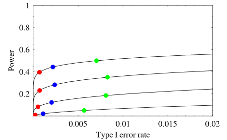
Figure 3: A plot of the power of the evidence ratio test for example 2, as a function of the probability of Type I error. Curves are shown for $N\sigma^{2}=2$ (lowest curve), increasing for each curve by a factor 2. The dots lie at evidence ratios of $e^{2}$(green), $e^{3}$ (blue) and $e^{4}$ (red).

Fig. 3 shows curves for the power versus significance level as a function of $N\sigma^{2}$. This parameter expresses the dependence of test performance on the amount of data ($N$) and the prior degree of difference between the proposed models ($\sigma$). In this plot, it is remarkable where standard choices of critical evidence ratio lie. Take $\ln{\cal E}_{c}=5$ for definiteness: at, say, $N\sigma^{2}=8$ we find the significance level to be $2\times 10^{-4}$ and the corresponding power to be $0.19$.

In words, this means that if we require the odds on $H_{1}$ to be 148 to 1 or stronger, then we will reject $H_{0}$ incorrectly only one time out of 5000 trials, and we will pick $H_{1}$ when we should only one time out of 5 trials. This is an excessively conservative decision procedure and parallels what we saw in the first example.

Evidently, we will need much smaller critical odds than 148 to 1 to get reasonable performance from this test. To re-emphasize, this is a function of the chosen critical evidence ratio, not the form of the test, which is intuitive. The problem is that $\ln{\cal E}$ is noisy for small amounts of data and cannot sustain such decisive tests as are implied by $\ln{\cal E}_{c}=5$ (for example). Fig. 4 illustrates this point.

This test might intuitively be derived without the evidence ratio, focusing on the test statistic $(\sum_{i}X_{i})^{2}$, where the square enters to allow for the possibility that the actual, non-zero $\mu$ can be be of either sign. For simplicity, consider the form $y$ we defined before, which is chi-square distributed (see equation 19). A simple test could be, reject $H_{0}$ if $y>y_{c}$, where the critical $y_{c}$ corresponds to some desired significance level or probability $p$ of Type I error. The power of this proposed test is conditional upon $\mu$. Marginalizing out $\mu$ with the Gaussian prior, as before, the forms of the power and significance level turn out to be identical to those based on the evidence ratio test. So the test is natural enough; the difficulty arises in choosing a sensible value for the critical evidence ratio. This is exactly the same difficulty that occurs in choosing the significance level in any classical test.

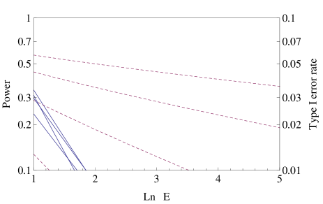
Figure 4: A plot of the power and significance levels of the evidence ratio test for example 2, as a function of the critical evidence ratio. Curves are shown for $N\sigma^{2}=2$ (lowest curve), increasing for each curve by a factor 2. Significance level is in blue, power in red. The changing slopes of the significance lines are real.

It might seem even more ‘natural’ for this problem to choose $\sum X_{i}^{2}$ as a test statistic. Working through the Neyman-Pearson analysis in this case is not possible analytically, as non-central chi-square distributions arise. However, a numerical analysis shows that this ‘natural’ procedure only performs better than the evidence ratio for small $N\sigma^{2}<3$. So the evidence ratio method is not trivially intuitive.

4.3 Conclusions from the Gaussian examples

These simple examples show that the odds that we calculate from the evidence ratio may not be useful for making decisions if we take account of statistical variations over an ensemble of datasets. A decisive threshold of $\ln{\cal E}=5$ can in many cases be exceeded only a small fraction of the time when $H_{1}$ is true, even when such a value is effectively impossible under $H_{0}$. In other words, the test is extremely safe (very hard to reject the null hypothesis incorrectly), but lacking in power (little ability to detect the alternative). This asymmetry between type I and type II performance seems undesirable, particularly because the problem is set up so that there are only two possibilities. If $H_{0}$ is clearly inconsistent with the data, then $H_{1}$ must be correct according to the problem as given – even if the Bayesian evidence ratio is only moderate. Again, this suggests that we should be free to challenge the statistical formulation and conclude that neither $H_{0}$ nor $H_{1}$ are correct. Fisher might have regarded this as the correct (less “wooden”) approach.

5 A LINE FITTING EXAMPLE

We now consider two more complex examples, where we are interested in which of two models is a better fit to spectral line data. We will use Monte Carlo simulation to assess the statistical scatter between different realizations of the data. We will consider two cases, one ‘nested’ (whether there is an extra component to a spectral line) and one not nested (whether a line has a Gaussian or Lorentzian profile).

Suppose we are trying to decide if a spectral feature is a single Gaussian (the null hypothesis $H_{0}$) or two Gaussians, of equal width, known separation, but unknown height ratio (the alternative hypothesis $H_{1}$). This is a nested model because if the height ratio is zero, $H_{1}$ reduces to $H_{0}$. The relevant parameters are the baseline; the height, width, and centre of the main line; and the height ratio for the subsidiary line. The models are:

$$H_{0}: y=\alpha_{1}+\alpha_{2}\exp\left(-\frac{1}{2\alpha_{3}^{2}}(x-\alpha_{4})^{2}\right)$$ (24)

$$H_{1}: y=\beta_{1}+\beta_{2}\exp\left(-\frac{1}{2\beta_{3}^{2}}(x-\beta_{4})^{2}\right)$$ (25)

$$+\beta_{5}\exp\left(-\frac{1}{2\beta_{3}^{2}}(x-\beta_{4}-3\beta_{3})^{2}\right).$$

The extra feature is located a known three standard deviations away from the main one. We also treat the noise levels as free parameters to be determined from the data; this is realistic because we may not know the noise level very well. We again assume that each model is a priori equally likely, and that the noise is normally distributed. The models need priors on the parameters, which we describe later. In the Neyman-Pearson framework, our decision rule for this example will be: accept $H_{1}$ if the evidence exceeds a critical value.

The Monte Carlo modelling process involves the following steps, some repeated.

1. To create the noise-free spectrum under $H_{0}$ we take $\alpha_{1}=\beta_{1}=0$, $\alpha_{2}=\beta_{2}=1$, $\alpha_{3}=\beta_{3}=1$, $\alpha_{4}=\beta_{4}=0$ in equation (24). The noise-free spectra are sampled on a pixel grid of spacing $1/5$ in the above units.

2. The noise-free spectrum under $H_{1}$ is created with the same parameters as for $H_{0}$ in equation (25) but the key parameter $\beta_{5}$, the strength of the satellite line, now enters. We will assume that the prior for $\beta_{5}$ is uniform between zero and 0.1, so we are looking for a satellite line that we expect to be at most 10% of the main line. The presence of this prior introduces a factor of 0.1 into the evidence ratio; we assume that the priors on the other parameters are the same for $H_{0}$ and $H_{1}$.

3. To estimate the Type I error rate, we generate simulated data with $H_{0}$ assumed true, adding Gaussian noise. We define the signal-to-noise ratio as the ratio of the peak level (unity) to the standard deviation of the added noise. We fit the forms for $H_{0}$ and $H_{1}$ to these simulated data and compute the evidence ratio in the sense ${\cal E}$ = evidence for $H_{1}$ / evidence for $H_{0}$, using the Laplace approximation. This gives the evidence ratio when the data are created on the assumption the $H_{0}$ is true.

4. To compute the power, we need to compute the evidence ratio using data generated data for the case where $H_{0}$ is false. We will do this by assuming that $H_{1}$ is true. We generate simulated data under $H_{1}$ by adding noise to the noise-free spectrum under $H_{1}$. Choosing the random values of $\beta_{5}$, the satellite line strength, from its prior naturally marginalizes the distribution of the evidence ratio over the range of prior assumed strengths for the satellite line (the evidence ratio is a very strong function of this line height).

5. We fit the forms for $H_{0}$ and $H_{1}$ again and compute the evidence ratio. Examples of the fits under $H_{0}$ and $H_{1}$ are shown in Fig. 5.

The use of the Laplace approximation is justified by examining the likelihood functions and finding them to be close to Gaussian – a check that should always be made.

Figure 5: Both panels show fits of Gaussians, where the bimodal model $H_{1}$ is favoured at odds of 20 to 1. In the upper panel, the fit of the model under $H_{1}$ is shown, in the lower, under $H_{0}$.

The trends of the evidence ratio with signal-to noise ratio are plotted in Fig. 6, which shows the median and the interquartile range for the log of the evidence ratio, plotted against the signal-to-noise ratio. We see that the evidence ratio or odds for $H_{0}$, if it is true, do not get very big compared to the odds for $H_{1}$. This is what we expect from a nested model, as $H_{1}$ can always do just as well as $H_{0}$, with only the Ockham penalty for extra complexity – not severe for only one extra parameter. It follows from our decision rule that the Type I error rate is quite low. Indeed, for the standard decisive ratio of $e^{5}=148$, the Type I error rates are exceedingly small – the decision rule is very conservative at these signal-to-noise ratios. On the other hand, clearly if $H_{1}$ is true we will often find values below the critical value and so the power is not large. Ultimately we can trace this to the width of the prior on the satellite line height; we are too vague about what we are looking for to have high power. This point arises again in the next example.

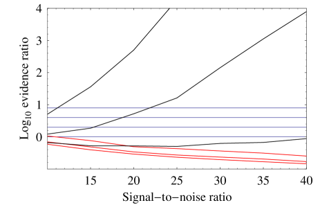
Figure 6: The evidence ratio for the first line-fitting example, in the sense evidence for $H_{1}$ / evidence for $H_{0}$, plotted against signal-to-noise ratio. These results include the effects of the priors that are described in the text. The red curve assumes $H_{0}$ is true (no satellite line) and the black curve assumes $H_{1}$ is true. The central curve is the median and the flanking solid lines are the 25th and 75th percentiles. 500 iterations were used at each noise level. The horizontal lines mark odds on $H_{1}$ that are even, 2:1, 4:1, and 8:1.

The utility of the proposed decision rule is summarized in Fig. 7, which shows the power and Type I error rate as a function of decision threshold (the chosen critical evidence ratio) and signal-to-noise ratio. This diagram is specific to the problem at hand, but interesting points emerge. Evidently, the combination of the critical evidence and the signal-to-noise ratio determines where the decision rule places one in the diagram. Standard decisive thresholds like $e^{5}$ result in low power and a very small Type I error rate – less than 1/500 with our number of repetitions of the Monte Carlo simulation. This may not be what is needed.

For comparison, we also apply a Bayesian Information Criterion (BIC; see e.g. Liddle 2007). In our case this means we pick the model with the smallest value of the normalized sum of squares plus the penalty term $\ln$(number of data points) $\times$ (number of model parameters). The number of data points is the number of spectral channels – evidently this number is somewhat vague as not all channels are equally informative.

The BIC rule, while offering no choices, sits in a useful place in the diagram for this relatively simple problem and is no worse in power than the evidence ratio. Finally, we note that different decision rules (for example, accepting $H_{0}$ if the evidence for it is bigger than the evidence for $H_{1}$) result in a different diagram.

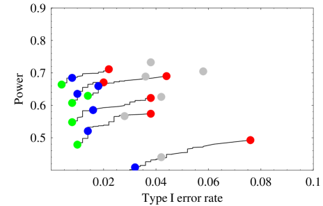
Figure 7: The power and Type I error rate for the first line-fitting example are shown for signal-to-noise ratios of 40 (topmost line), 35, 30… The critical ratio varies along each line, with points indicating a critical evidence ratio in favour of $H_{1}$ of 2 (red), 4 (blue) and 8 (green). Grey points are for the simple case of picking the model with the smaller BIC. At each signal-to-noise ratio – $\beta_{5}$ combination, 500 iterations were used. The Type I error rates are therefore not reliable near $1/500$ – the power should be zero for if the Type I error rate is zero, but the curves are too steep near the origin to resolve properly with Monte Carlo.

For a second example, we consider trying to decide if a line profile is Gaussian ($H_{0}$) or Lorentzian ($H_{1}$). Here we have

$$H_{0}: y=\alpha_{1}+\alpha_{2}\exp\left(-\frac{1}{2\alpha_{3}^{2}}(x-\alpha_{4})^{2}\right)$$ (26)

$$H_{1}: y=\beta_{1}+{\beta_{2}\over 1+(x-\beta_{4})^{2}/\beta_{3}^{2}}.$$ (27)

The simulation proceeds very much as in the first case, except that we assume the priors are the same for the two models; this is justifiable since each of the parameters has a very similar effect in either model. We return to the priors later. The decision rule is, accept $H_{1}$ (the Lorentzian) if the evidence for it is bigger.

Fig. 8 shows examples of fits. Because the models are not nested, and there is no Ockham factor in play, the odds (at reasonable signal-to-noise ratios) are much stronger than in the previous example. Fig. 9 shows the trends of evidence ratio with signal-to-noise. There is much less spread in this case because it lacks the additional variability introduced into the previous example by the prior on the height of the satellite line.

Figure 8: This shows a case where a Lorentzian (lower panel) is favoured over a Gaussian (upper panel) at odds of 60:1. These impressive odds result from exponentiating small differences in the wings of the lines.

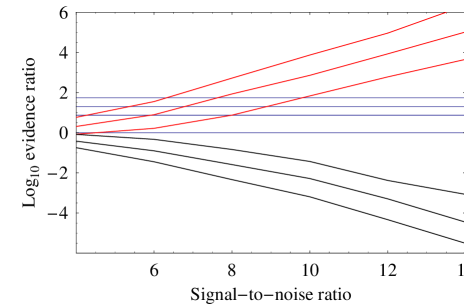
Figure 9: The evidence ratio, in the sense evidence for $H_{0}$ / evidence for $H_{1}$, for the second line-fitting example, plotted against signal-to-noise ratio. The red curve assumes $H_{0}$ is true. The central curve is the median and the flanking solid lines are the 25th and 75th percentiles. 500 iterations were used at each noise level. The horizontal lines mark odds on $H_{1}$ that are even, $e^{2}$:1, $e^{3}$:1 and $e^{4}$:1.

Fig. 10 shows the Type I error rates and powers in the same format as before. Performance is better (lower Type I error rate, and higher power, at the same signal-to-noise ratio), reflecting the fact that the two models are more distinct. Unlike the previous example, the BIC gives better power but worse Type I error rate.

Two points emerge that are more specific to the Bayesian context. One is the way we have formulated the decision rule, in terms of accepting $H_{1}$. In the double-line example, it is clear than $H_{1}$ is the more complex model, and classically we would probably have focused on whether or not we accepted $H_{0}$. The decision rule, ‘accept $H_{0}$ if the evidence for it is bigger than for $H_{1}$’ gives a different power – Type I error rate tradeoff. The same is true for the second example, where this formulation (accepting the Gaussian, in that case) gives a much higher power, and much worse Type I error rate.

The second point relates to the role of priors. There is no Ockham factor at work in the second example – but the odds that arise seem implausibly large, just looking at the fits. This happens because in the simulations we fit exactly the right model to the fake data. A related point is that our model space contains either $H_{0}$ or $H_{1}$ and nothing else. In reality it seems more likely that we would know $H_{0}$, the default, null, or starting hypothesis fairly well, but the alternative might be rather vague Again, this reiterates the lesson of the Gaussian examples, where we warned against adopting too restricted a set of models.

We can see the effects of this by a simple change to the Monte Carlo modelling. For the case $H_{1}$ true, we generate the fake data from the simple Lorentzian. We then fit a more complex model, a Lorentzian plus a quadratic baseline $ax+bx^{2}$. This corresponds to a case where Nature is simple, but we do not know this. Without accounting for priors, we find the odds on the Lorentzian model drop by five orders of magnitude. The factors accounting for the priors on $a$ and $b$ can recover much of this. For example, if we think in advance $ax+bx^{2}$ should be less than the line height (1) over the range of the data ($\pm 10$) then we expect the prior range in $a$ to be $\simeq 0.1$ and in $b$ to be $\simeq 0.01$, which allows us to recover three orders of magnitude in the evidence ratio. The second panel of Fig. 10 incorporates the nett loss of two orders of magnitude in the odds for $H_{1}$, and we see a large effect in the power. The Type I error rate remains the same because we have not changed $H_{0}$ in any way, reflecting its assumed role as the default, better-defined hypothesis. This part of the example shows how model uncertainty may play a large role in the quality of decisions made with a limited suite of options.

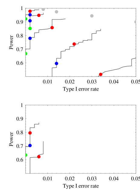
Figure 10: The power and Type I error rate for the second line-fitting example are shown for signal-to-noise ratios of 40 (topmost line), 35, 30… The critical ratio varies along each line, with points indicating critical odds on $H_{0}$ of $e^{2}$:1 (red), $e^{3}$:1 (blue) and $e^{4}$:1 (green). Grey points are for the simple case of picking the model with the smaller BIC. The upper diagram has no quadratic baseline; the lower includes this as a possibility, as described in the text. Not all signal-to-noise ratios yield curves that lie in the plotted ranges of power and Type I error rate.

5.1 Conclusions from the Monte Carlo examples

The direct simulations clarify some key aspects of the evidence ratio method. The role of the prior is apparent; uncertainty in our model parameters can range from sampling noise dominated (spread in prior values $\gg$ spread due to measurement error) through to noise-dominated. The meta-problem of model uncertainty is also illustrated. A spurious restriction of the range of applicable models is punished by equally bogus levels of certainty. In this regard, simple goodness-of-fit criteria have much to offer as complements to formal procedures of model choice.

Treating the evidence ratio as a statistic shows that it has familiar features. Choosing a ‘decisive’ value, in the face of poor signal-to-noise ratio or similar models, results in conservative decision procedures with low power to pick alternatives. Really this is just a reprocessing of the lack of information in the data, but the evidence ratio encodes this fact in an obscure way. There is no obvious relationship between the posterior odds, the Type I error rate, or the power: signal-to-noise trumps all of these.

6 Why does the evidence ratio scatter so much?

We have discussed at length a number of specific examples, which raise various questions concerning the evidence ratio methodology. The common feature has been the large dispersion in the evidence ratio, and the associated poor performance as a statistical tool for decision making. We now have to ask if our examples are just pathological cases, or if there is a general reason for the large scatter in the evidence ratio.

Suppose we are dealing with Gaussian statistics and we are fitting functions $y=f(x,\vec{\alpha})$ and $y=g(x,\vec{\beta})$ to data $Y_{i}$, with known noise, at a set of points $x_{i}$. In the Laplace approximation, the statistics of the evidence ratio are largely dominated by the likelihood ratio

$${\cal L}=\frac{\exp\left(-\frac{1}{2}\chi^{2}(\vec{\alpha^{*}})\right)}{\exp\left(-\frac{1}{2}\chi^{2}(\vec{\beta^{*}})\right)},$$ (28)

where the star superscript denotes the maximum likelihood value of the parameters. The logarithm of this is

$$-\frac{1}{2\sigma^{2}}\left(\sum_{i}(f(x_{i},\vec{\alpha^{*}})-Y_{i})^{2}-\sum_{i}(g(x_{i},\vec{\beta^{*}})-Y_{i})^{2}\right).$$ (29)

Collecting terms, the contribution at each $i$ to the summation is

$$\left(f(x_{i},\vec{\alpha^{*}})^{2}-(g(x_{i},\vec{\beta^{*}})^{2}\right)+\left(2(f(x_{i},\vec{\alpha^{*}})-g(x_{i},\vec{\beta^{*}}))Y_{i}\right).$$ (30)

If $f$ (for example) is the correct model, then $Y_{i}\simeq f(x_{i},\vec{\alpha^{*}})+Z_{i},$ where $Z_{i}$ is a Gaussian variate by assumption. Introducing the distance $h$ between the models by $h(x_{i},\vec{\alpha^{*}},\vec{\beta^{*}})=f(x_{i},\vec{\alpha^{*}})-g(x_{i},\vec{\beta^{*}})$ we see we have a sum of terms in which the stochastic component is of the form

$$\delta\ln{\cal L}=\sum_{i}h(x_{i},\vec{\alpha^{*}},\vec{\beta^{*}})Z_{i}/\sigma^{2},$$ (31)

where $\sigma$ denotes the rms noise.

We therefore expect the logarithm of the evidence ratio (the log odds) to have a Gaussian distribution, with the width of this Gaussian determined by the detail of the distance function $h.$ There are some special cases where this width might be small. One is where the ‘incorrect’ model $g$ is just the ‘correct’ model $f$, plus some term that is linear in the parameters. This of course would be true for any pair of linear models where $g$ was a more complicated version of $f$. In such a case, $h$ can be small. More generally, if $f$ and $g$ are nested models, with a parameter that is free to be determined in $f$ but fixed in $g$, then $h$ will also be small if the fixed value is close to the optimum.

In general, however, apart from special cases, we should expect that the log-odds will have a degree of variance for different realizations of the data. The extent of the variance will depend on the details of the models being compared but can be considerable for commonplace problems. Since the variations in $h$ that will be consistent with either model will naturally be $\sim\sigma$, this suggests a scatter in $\ln{\cal E}$ of order unity, as found in our examples.

Finally we note the similarity of this treatment to the classical likelihood ratio test. In this test, the logarithm of the ratio of maximum likelihoods is found to be distributed like chi-square, if the models are nested. The relevance for us is that here we have a test statistic that is of very similar form to the evidence ratio, and which will inevitably show considerable scatter – although the exact degree of scatter must be calculated in individual cases, most simply by Monte Carlo simulation.

7 Summary and conclusions

We have discussed the application of the Bayesian evidence ratio to some simple problems of model selection, which are illustrate issues encountered in astronomical applications. We have treated the evidence ratio as a statistic that can be computed for a given dataset. Using analytical arguments and Monte Carlo simulation, we have investigated the distribution of evidence ratio values that results from an ensemble of experiments. Although the Bayesian approach treats the data as given, our data are but one sample of a range of possibilities. The evidence ratio calculation indeed assumes that we know the distribution of the data, so a calculation that incorporates this random element is always possible. All experiments could in principle be repeated (even the single datum of our Universe, if we accept the Landscape picture – e.g. Susskind 2003).

In the examples we have investigated, we find that the evidence ratio has a large dispersion about its ensemble average, and we have given arguments to suggest that such behaviour is likely to be general. We therefore suggest that one should compute not only the value of ${\cal E}$, but also its distribution.

Of course, at any one time, we have to work with the data that exist, and nothing that we write here should be taken as challenging the fundamental Bayesian paradigm: modulo the often unjustly neglected priors on model classes, the evidence ratio does express our full knowledge of the relative odds on different models. But when one moves beyond this statement to a decision (the evidence is large enough, so I will build a factory to produce a new drug, or I will launch a new Great Observatory), then we need to know more about the evidence than a single numerical value.

This point is of particular importance in calculations that attempt to predict the potential decisiveness of future experiments, as in e.g. Heavens et al. (2007) or Trotta (2007b). The expected evidence ratio for a given experiment, $\langle{\cal E}\rangle$, is an interesting quantity to know – but one may not want to choose an experimental strategy that maximises this quantity, if the price is an increased scatter.

The ‘noisy’ nature of the evidence ratio has a number of implications. At the practical level, there is a limit to how much effort it is worth investing in numerical algorithms for accurate computation of the evidence ratio: arguably, there is no point in evaluating ${\cal E}$ to better than a factor of 2 numerical precision. The Laplace approximation may be useful here, as may judicious use of approximate combinations of models (sometimes called ‘toy’ models, although this term can be an injustice).

Most seriously, the scatter in ${\cal E}$ means that it is inevitable that a good fraction of experiments will fail to find decisive evidence in favour of a more complex model, even when it is true (a large ‘Type II’ error rate, or low power). In such cases, do we accept that the simpler model is still an acceptable description of the data? The problem with this conclusion is that performance of the evidence ratio when viewed as a statistic seems to be asymmetric between Type I and Type II errors. There may well exist levels of evidence that are far from being decisively in favour of a complex model (${\cal E}\sim 1$), and are yet close to impossible on a simpler model. It such circumstances, it hardly seems sensible to persist with the simple model.

This reasoning is certainly reminiscent of the current controversy over whether a scale-invariant spectrum of cosmological mass fluctuations is ruled out (only moderate evidence in favour of tilted models $\ln{\cal E}=2.8$, according to Trotta 2007a, even though the observed deviation from $n=1$ is ‘$3.3\sigma$’). It would be interesting to study this situation using the approach of Monte Carlo realizations that we have advocated here, to see what the evidence ratio is really telling us.

In such circumstances, where the evidence ratio fails to discriminate clearly between alternative models, and yet the available data are a poor match to the null model, we have to question whether the problem is correctly formulated. While the null hypothesis will normally be rather specific, the alternative can be vague, and difficult to reduce to a single model (a point made by Efstathiou 2008 in his critique of the evidence ratio approach). But if the null model gives a poor fit to the data to hand, we have good reason to believe that we need another model, even if the the evidence ratio is unable to convince us that this must be the supplied alternative. The strength of the Bayesian approach is that it focuses our attention on the actual models we are considering. But without a goodness-of-fit test, the result may simply demonstrate that we lack the imagination to create a sufficiently exhaustive set of models.

REFERENCES

Berger J.O., Sellke T., 1987. J. Am. Stat. Assoc., 82. 112.

Efstathiou G., 2008, MNRAS 388, 1314

Feroz F., Hobson M.P., Bridges M., 2009, MNRAS, 398, 1601

Fisher, R.A., 1956. In Chapter 4 of Statistical Methods and Scientific Inference Edinburgh: Oliver & Boyd.

Gelman A., Hill J., 2007, “Data Analysis Using Regression and Multilevel/Hierarchical Models, Cambridge University Press

Gregory P.C., 2005, ApJ, 631, 1198

Heavens A.F., Kitching T.D, Verde L., 2007, MNRAS, 380, 1029

Hobson M.P., Jaffe A.H., Liddle A.R., Mukherjee P. & Parkinson D., 2010, Bayesian methods in cosmology, Cambridge University Press

Jaynes E.T., 2003, Probability Theory, Cambridge University Press

Jeffreys H., 1961, Theory of Probability, Oxford University Press

Liddle A.R., 2004, MNRAS, 351, L49

Liddle A.R., 2004, MNRAS, 377, L74

Lindley D.V., 1957, Biometrika, 44, 187

Niarchou A., Jaffe A.H, Pogosian L., 2004. Phys. Rev. D 69, 063515

Mackay D.J.C., 2003, Information theory, inference, and learning algorithms, Cambridge University Press

Mukherjee P., Parkinson D., Liddle, A.R., 2006, ApJ, 638, L51

Sellke T., Bayarri M.J., Berger J.O., 2001. The American Statistician, 55, 62.

Skilling J., 2004, in Bayesian inference and maximum entropy methods in science and engineering, AIP Conference Proceedings, 735, 395

Susskind L., 2003, arXiv:hep-th/0302219

Tegmark M., Taylor A.N., Heavens A.F., 1997, ApJ, 480, 22

Trotta R., 2007a, MNRAS, 378, 72

Trotta R., 2007b, MNRAS, 378, 819

Trotta R., 2008, Contemp. Phys. 49, 71